Neural Network and Dynamic Inversion Based Adaptive Control for a HALE-UAV against Icing Effects

Abstract

In the past few decades, in-flight icing has become a common problem for many missions, potentially leading to a reduction in control effectiveness and flight stability, which would threaten flight safety. One of the most popular methods to address this problem is adaptive control. This paper establishes a dynamic model of an iced high-altitude long-endurance unmanned aerial vehicle (HALE-UAV) with disturbance and measurement noise. Then, by combining multilayer perceptrons (MLP) with a nonlinear dynamic inversion (NDI) controller, we propose an MLP-NDI controller to compensate for online inversion errors and provide a brief proof of control stability. Two experiments were conducted: on one hand, we compared the MLP-NDI controller with other typical controllers; on the other hand, we evaluated its robustness and adaptiveness under different icing conditions. Results indicate that the MLP-NDI controller outperforms other typical controllers with higher tracking accuracy and exhibits strong robustness in the presence of icing errors and measurement noise, which has huge potential to ensure flight safety.

1. Introduction

In-flight icing poses a significant threat to flight safety and can result in fatal accidents. The effects of ice accretion on wings and control surfaces can greatly reduce lift and increase drag forces, and may even cause structural imbalances [1]. This will lead to a decrease in flight stability and controllability [2]. Statistic data from American Safety Advisor showed that 12% of all weather-resulted accidents were caused by icing and 92% of the ice-induced accidents were in-flight icing [3].

To mitigate the risks of in-flight icing, two main approaches are currently used in practice. The first approach provides pilots with detailed weather information before the flight mission to avoid potential icing conditions. The second approach relies on classical icing protection systems (IPSs) which employ deicing and anti-icing methods to remove or inhibit ice accretion, respectively [4]. Various deicing methods have been incorporated into IPSs, including bleeding hot engine exhaust to counteract frigid icing conditions and using inflatable boots to break off the accumulated ice. Chemical reagents have been considered as an effective anti-icing method in recent years [5]. Despite the implementation of various engineering measures, accidents resulting from in-flight icing continue to occur. In October 1994, an accident involving American Eagle ATR-72 near Roselawn, Indiana, resulted in the death of 68 individuals [6]. Similarly, China Eastern Airlines Flight 5210 (CRJ-200) crashed after takeoff in Baotou City in November 2004 and left 55 dead. In 2009, Air France Flight 447 (A330) crashed over the Atlantic Ocean; all the passengers on board were lost [7,8]. These accidents highlight the inadequacy of relying solely on IPS for ensuring flight safety. A four-year tailplane icing program (TIP) was then cosponsored by NASA and FAA after the ATR-72 accident [9], which led to the proposal of the icing management system (IMS) by Bragg et al. [10]. An IMS firstly takes into account the deterioration of aerodynamic derivatives and can automatically activate the traditional IPS devices. It also introduces a configuration into the flight control laws to restrict the maneuver within a proper margin of safety.

For HALE-UAVs, ice accretion occurs during the climb stage of flight, particularly below 25,000 feet altitude. These aircraft often fly through areas with high humidity or sufficient water content in the clouds, which are naturally icing high-risk regions or strong icing conditions [11]. For these aircraft, the IPS cannot be activated by a human pilot, it only relies on the IMS. Inspired by Bragg, recent research on HALE-UAV icing has primarily focused on two key areas. The first area involves online estimation of the effects of icing accretion [12], while the second area involves developing an ice-tolerant control law. Since the icing effects can be considered as a part of the modeling error in many ways, the use of fault-tolerant control (FTC) can bring better results [13]. Jiang and Yu divided FTC into passive and active types and gave their comparison results [14]. Passive approaches such as robust control are relatively easy to implement, but can only handle limited faults. On the other hand, active approaches perform better when dealing with various faults, and a lot of research was therefore conducted on it [15,16,17,18,19,20,21,22,23,24]. Ru proposed a multiple model control method that utilizes a finite set of linear models to express the system in different conditions [16]. Additionally, an online processor that determines which model to use based on Kalman filters was also employed. Furthermore, Verhaegen et al. discussed three typical multiple model controllers [17], but the oscillation problem in model switching still needs further improvements. Shtessel constructed a two-loop cascade structure of sliding mode control (SMC) by using standard sliding mode functions [18]. It is theoretically able to handle all structural errors less than the prior-assumed uncertainty, although limitations still exist. For instance, there must be one, and only one, control surface for every controlled variable, and we can never afford to lose it [17]. With the enhancement of hardware computing power in recent years, model-predictive control (MPC) has become more popular. It can effectively control a multi-input multi-output (MIMO) system with constraints as long as a reference model exists [19]. However, obtaining an accurate system without modeling errors remains a critical challenge for MPC.

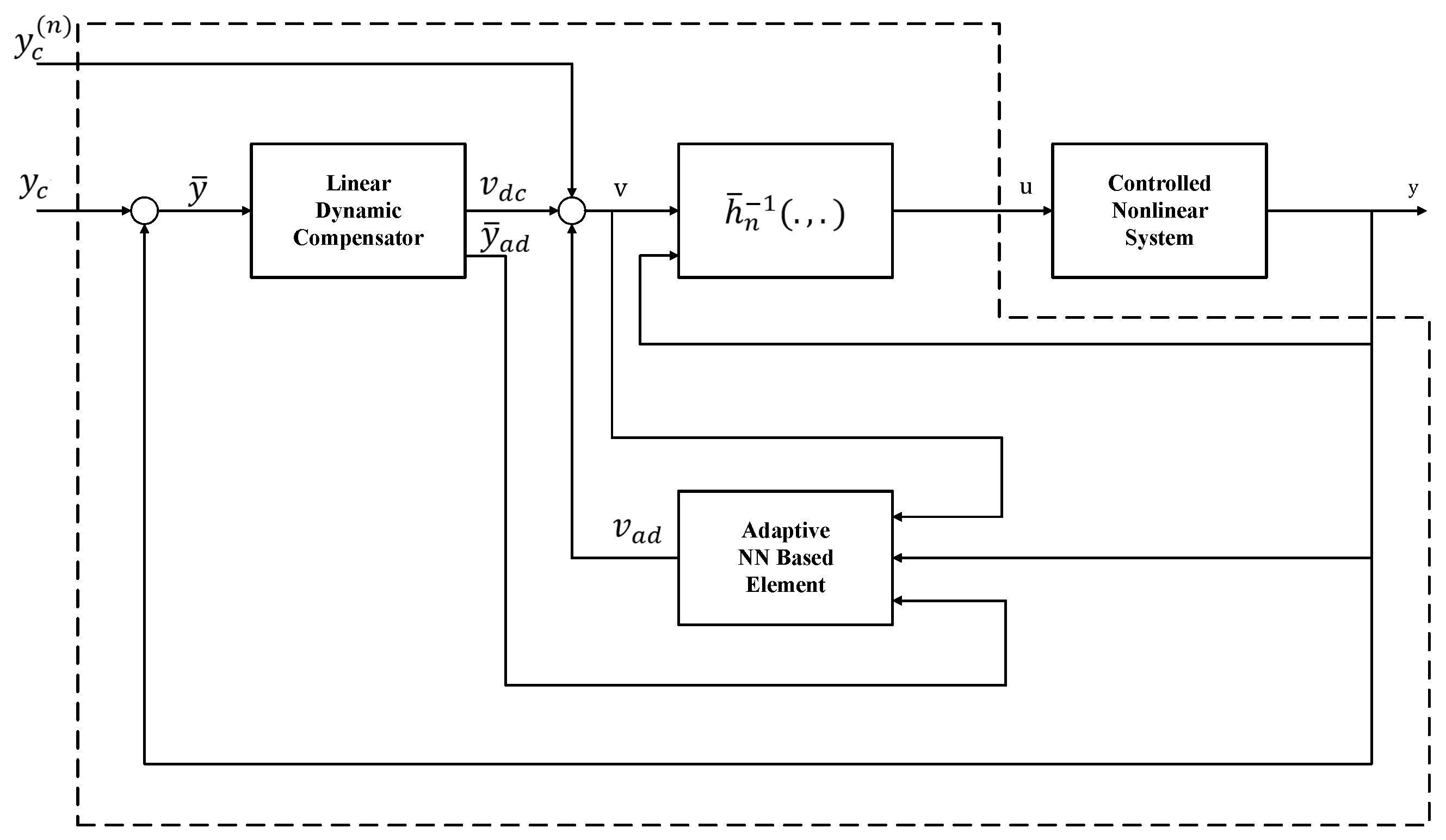
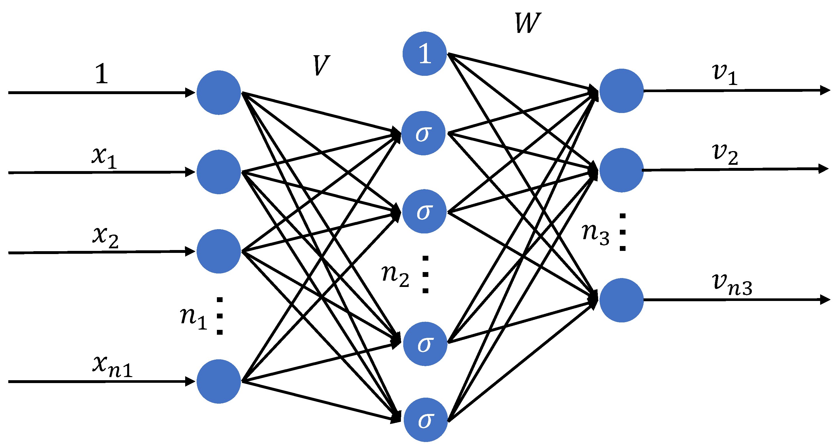
In recent years, neural networks have also been widely used due to their good global approximation properties for nonlinear functions [20], and are therefore suitable for adaptive compensation. Calise et al. firstly applied this approach to control a rigid robot arm and successfully incorporated it into a feedback linearization framework [21,22,23], as shown in Figure 1. Shin et al. also proposed a neural-network-based adaptive backstepping controller and achieved good performance [24]. Though feedback linearization is an effective control technology, the linearized model for a six-DOF icing aircraft can be highly time-varying, and compensation for this approximate linear system can vary significantly in continuous time steps. To address this issue, this paper combines the nonlinear inversion method with neural networks and divides the entire system into three-layer subsystems. This decoupling stabilizes the ideal compensation and enhances the neural network’s learning effect.

To be specific, the highlights of our work are

• We established a comprehensive fixed-wing icing model of HALE-UAV considering wind disturbance and sensor noise.
• We proposed an ice-tolerant control structure by combining multilayer perceptrons with the nonlinear dynamic inverse method (MLP-NDI controller) to provide robust compensation for the nonlinear and time-varying icing effects.
• We conducted extensive comparisons between the MLP-NDI controller and three typical controllers, demonstrating its superior performance in terms of stability, accuracy, and robustness.
• We explored the robustness and verified the effectiveness of an MLP-NDI controller under various icing scenarios.

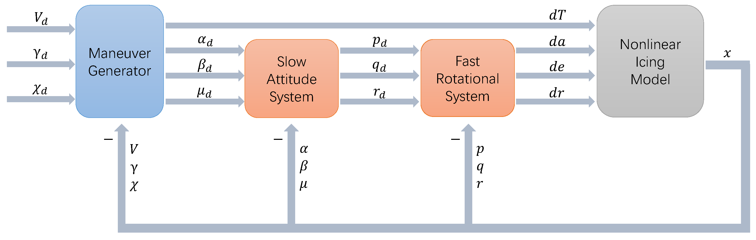
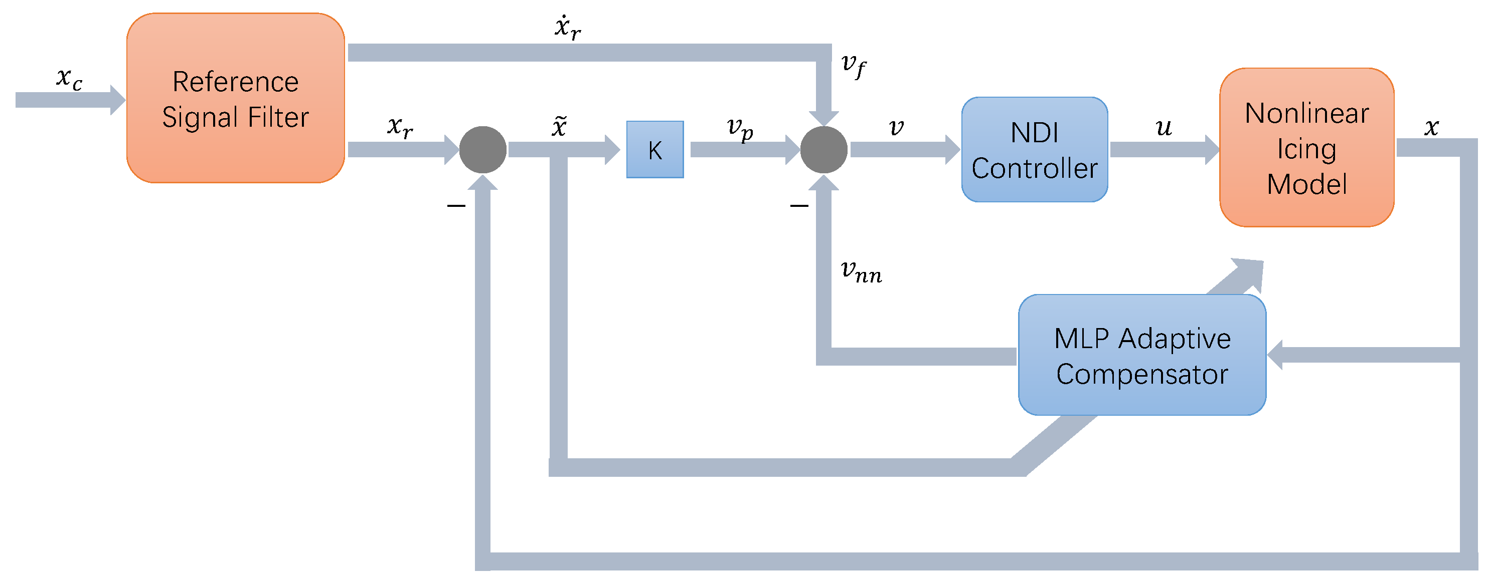
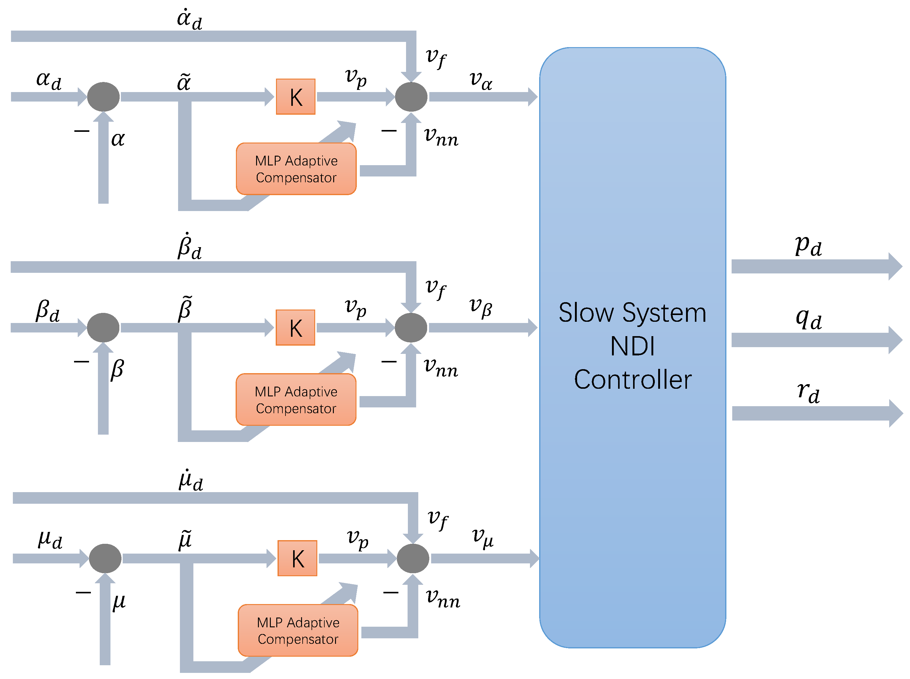
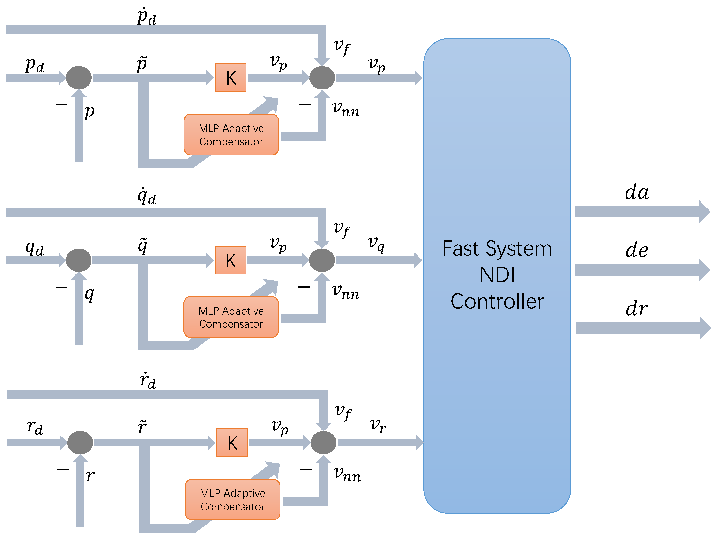
The remaining parts of this paper are organized as follows. Section 2 analyses the icing effect on flight dynamics based on the DHC-6 nonlinear model. Section 3 gives the overall control architecture of the NDI with MLP compensator and applies the MLP-NDI controller to icing flight control, including the icing effect model. Section 4 provides the simulation results and analysis, which demonstrate the feasibility of the MLP-NDI with a preliminary assessment of its control performance. Finally, a conclusion is presented in Section 5.

2. Flight Dynamic Model

2.1. Icing Effects on Flight Dynamic

Bragg et al. proposed a classical model of icing effects on a fixed-wing aircraft [25]:

$$C_{*}^{iced}=C_{*}^{clean}·(1+{\eta }_{ice}{k}_{C_{*}})$$

(1)

where $C_{*}^{clean},C_{*}^{iced}$ are the same aerodynamic derivative before and after icing. ${\eta }_{ice}$ is an icing severity factor, and $k_{C_{*}}$ is the associated slope determined from the parameter being modified.

Considering the lack of available data on icing-related research for fixed-wing UAVs and the similarity in the aerodynamic design to fixed-wing aircrafts, this paper established the icing model utilizing open access data of the Twin Otter icing research plane DHC-6 (Figure 2), which has been extensively tested by NASA [26].

Table 1. Dynamic parameters of Twin Otter in clean and iced configurations.

(a)
	$C_{Z0}$	$C_{Z\alpha }$	$C_{Zq}$	$C_{Z\delta e}$	$C_{x0}$	K	$C_{m0}$	$C_{m\alpha }$	$C_{mq}$	$C_{m\delta e}$
Clean	−0.380	−5.660	−19.970	−0.608	−0.041	0.052	0.008	−1.310	−34.200	−1.740
Wing	−0.380	−5.342	−19.700	−0.594	−0.050	0.053	0.008	−1.285	−33.000	−1.709
Tail	−0.380	−5.520	−19.700	−0.565	−0.046	0.053	0.008	−1.263	−33.000	−1.593
Both	−0.380	−5.094	−19.700	−0.550	−0.062	0.057	0.008	−1.180	−33.000	−1.566
(b)
	$C_{Y\beta }$	$C_{Yp}$	$C_{Yr}$	$C_{Y\delta r}$	$C_{l\beta }$	$C_{lp}$	$C_{lr}$	$C_{l\delta a}$	$C_{l\delta r}$	$C_{n\beta }$	$C_{np}$	$C_{nr}$	$C_{n\delta a}$	$C_{n\delta r}$
Clean	−0.60	−0.20	0.40	0.150	−0.080	−0.50	0.06	−0.150	0.0150	0.10	−0.06	−0.180	−0.12	−0.001
Both	−0.48	−0.20	0.40	0.135	−0.072	−0.45	0.06	−0.135	0.0138	0.08	−0.06	−0.169	−0.11	−0.001

provides detailed clean and iced parameters for DHC-6, which were captured at ${\eta }_{ice}=0$ and ${\eta }_{ice}=0.2$ [5]. $k_{C_{*}}$ could then be calculated as the associated slope from this particular data point under different icing locations (wing, tail, and wing–tail both icing).

To accurately simulate the in-flight icing process, we utilized a time-varying model that takes into account the accumulation of in-flight icing with time [27,28].

$$\frac{d}{dt}{\eta }_{ice}=N_1(1+N_2{\eta }_{ice})C_{\eta }$$

(2)

where $C_{\eta }$ denotes the conduciveness of the atmosphere to icing. The coefficients $N_1,N_2$ are determined from an assumed icing severity profile characterized by the icing duration time, $T_{cld}$, and the final and middle values of the icing severity, ${\eta }_{ice}\left(T_{cld}\right)$ and ${\eta }_{ice}(T_{cld}/2)$, respectively. For all cases in this paper, the conduciveness of the atmosphere to icing is assumed to be a raised cosine as follows:

$$C_{\eta }\left(t\right)=\frac{1}{2}[1-cos\left(\frac{2\pi t}{T_{cld}}\right)]+d_{\eta }$$

(3)

Note that there exists an uncertainty $d_{\eta }$ in the conduciveness model; here, we consider a zero-bias situation with $d_{\eta }=0$. We then have

$$\begin{array}{cc}\hfill N_2& =\frac{{\eta }_{ice}\left(T_{cld}\right)-2{\eta }_{ice}(T_{cld}/2)}{{\left[{\eta }_{ice}(T_{cld}/2)\right]}^2}\hfill \\ \hfill N_1& =\frac{2}{N_2{T}_{cld}}ln[1+N_2{\eta }_{ice}\left(T_{cld}\right)]\hfill \end{array}$$

(4)

Besides the clean case (no ice), two typical scenarios are investigated in this paper. Figure 3 shows the change of ${\eta }_{ice}$ in different cases. For the moderate icing case, $T_{cld}=360,{\eta }_{ice}\left(T_{cld}\right)=0.2,{\eta }_{ice}(T_{cld}/2)=0.12$. For the severe/rapid icing case, $T_{cld}=120$, ${\eta }_{ice}\left(T_{cld}\right)=0.9,{\eta }_{ice}(T_{cld}/2)=0.5$. Both cases have the same start of ice accretion at $t=30$ with wing–tail both icing and the whole experiment lasts for 542 s, which would be sufficient to fully evaluate different controllers’ performance.

2.2. Nonlinear Dynamics

In this paper, the six-DOF motion equations of an HALE-UAV were established in the body axis [29]. To ensure consistency across all testing cases, the simulations were initialized from a trimmed point of steady, level flight at an altitude of 3000 m and a velocity of 60 m/s. At the start of the simulation, the icing severity of the HALE-UAV was 0, and all icing effects began at $t=30$. Throughout the simulation period, the icing severity was modeled using Equations (2)–(4) with different trends shown in Figure 3.

2.3. Disturbances and Measurement Noise

The effects of disturbance and measurement noise on an icing fixed-wing aircraft were first considered by Bragg et al. [25], after which a lot of further research has been conducted [4,5,27,28,30]. In this paper, we modeled disturbance as a zero-mean, band-limited white Gaussian noise with 50 Hz bandwidth. Since the linearized motion transform between the UAV’s wind and body axis is $V\approx u,\alpha \approx w/V,\beta \approx v/V$, the intensity of disturbance is modeled as a perturbation to the velocities in body axes with a severe case of $d_p={\dot{u}}_w={\dot{v}}_w={\dot{w}}_w=0.40$ g.

$$\begin{array}{cc}\hfill {\dot{V}}_w& \approx {\dot{u}}_w\hfill \\ \hfill {\dot{\alpha }}_w& \approx {\dot{w}}_w/V\hfill \\ \hfill {\dot{\beta }}_w& \approx {\dot{v}}_w/V\hfill \end{array}$$

(5)

Similarly, the measurement noise is also constructed as a zero-mean, band-limited Gaussian noise. The noise intensities, which depend largely on the UAV’s sensor resolution, were picked from the detailed information of in-flight instruments [26]. Some of these are listed in

Table 2. Part of the sensor resolution of Twin Otter.

$\mathit{p}/\mathit{q}$	r	$\mathit{\theta }$	$\mathit{\varphi }$	$\mathit{\alpha }/\mathit{\beta }$	V	H	$\mathit{\delta }\mathit{a}$	$\mathit{\delta }\mathit{e}$	$\mathit{\delta }\mathit{r}$
0.0167	0.0138	0.0293	0.0439	0.003	0.0391	2.4994	0.0091	0.0128	0.008

.

3. MLP-NDI Adaptive Control

3.1. Feedback Inversion

Consider a nonlinear dynamic system

$$\dot{x}=f(x,u)$$

(6)

where $x\in R^m$ represents the state vector and $u\in R^n$ represents the control vector. Define a pseudo-control vector v, which satisfies

$$\begin{array}{cc}\hfill \dot{x}& =v\hfill \\ \hfill v=& f(x,u)\hfill \end{array}$$

(7)

The inverse system can then be written as

$$\widehat{u}={\widehat{f}}^{-1}(x,v)$$

(8)

where ${\widehat{f}}^{-1}$ represents the approximation of inverse model. Since it is always hard to obtain the explicit model, the inversion error $\Delta$ is defined as follows:

$$\Delta (x,u)=f(x,\widehat{u})-\widehat{f}(x,\widehat{u})$$

(9)

The closed-loop dynamic system then becomes

$$\dot{x}=v+\Delta (x,u)$$

(10)

Mathematically speaking, the inversion error is a function that is nonlinear, time-varying, and dependent on the command signal, states, and inputs, making it difficult to model precisely under a severe icing scenario. Furthermore, the aerodynamic derivatives of icing conditions in Table 1 can only be used for modeling purposes. Consequently, the control law should be based solely on the parameters of the clean aircraft. It is therefore theoretically challenging to eliminate the inversion error within a dynamic inverse framework alone.

Noticing the good approximation property of neural networks for continuous nonlinear functions, an MLP can be employed here as an error compensator. By adding an additional term $v_{nn}$ on the pseudo-control signal v at each moment, the inversion error can be sufficiently mitigated. The resulting control structure is depicted in Figure 4.

The pseudo-control signal v is then composed of three parts: a derivative term of the reference signal $v_f$, a proportional term of the error $v_p$, and an adaptive compensation term $v_{nn}$

$$v=v_f+v_p-v_{nn}$$

(11)

where

$$\begin{gathered} v_f={\dot{x}}_r \\ {v}_p=K(x{}_r-x)=K\tilde{x} \end{gathered}$$

(12)

Substituting (11) and (12) into (10), the error system can be obtained as follows:

$$\dot{\tilde{x}}=-K\tilde{x}+v_{nn}-\Delta$$

(13)

Hence, if the adaptive compensator can fully offset the inversion error, the error system would then be asymptotically stable.

3.2. MLP-Based Adaptive Compensator

In this paper, a multilayer perceptron was applied to reconstruct the inversion error [31]. As shown in Figure 5, an input–output map of the MLP structure can be written as

$$v_{nn,k}={\theta }_{Wk}+\sum _{j=1}^{n_2}{w}_{jk}\sigma \left(z_j\right)$$

(14)

where $k=1,2,\dots ,n_3$, and

$$\sigma \left(z_j\right)=\sigma ({\theta }_{Vj}+\sum _{i=1}^{n_1}{v}_{ij}{x}_i)$$

(15)

where $n_1,n_2,n_3$, respectively, represent the input size, the hidden layer size, and the output size of the neural network. $w_{jk},v_{ij}$ are the layer weights and $\theta$ is the bias. $\sigma \left(z\right)$ is an activation function, and, here, we chose the sigmoid function defined as

$$\sigma \left(z\right)=\frac{1}{1+e^{-z}}$$

(16)

In addition, we define two weight matrices $V\in R^{(1+n_1)\times n_2},W\in R^{(1+n_2)\times n_3}$

$$\begin{array}{c}\hfill V=\left[\begin{array}{ccc}{\theta }_{V1}& \cdots & {\theta }_{V{n}_2}\\ v_{11}& \cdots & v_{1n_2}\\ ⋮& \ddots & ⋮\\ v_{n_{1}1}& \cdots & v_{n_1{n}_2}\end{array}\right]\\ \hfill W=\left[\begin{array}{ccc}{\theta }_{W1}& \cdots & {\theta }_{W{n}_3}\\ v_{11}& \cdots & v_{1n_3}\\ ⋮& \ddots & ⋮\\ v_{n_{2}1}& \cdots & v_{n_2{n}_3}\end{array}\right]\end{array}$$

(17)

and two augmented vectors $\mathit{x}\in R^{(1+n_1)},\mathit{\sigma }\in R^{(1+n_2)}$

$$\begin{array}{c}\hfill \mathit{x}={\left[\begin{array}{cccc}1& x_1& \cdots & x_{n_1}\end{array}\right]}^T\\ \hfill \mathit{\sigma }={\left[\begin{array}{cccc}1& {\sigma }_1& \cdots & {\sigma }_{n_2}\end{array}\right]}^T\end{array}$$

(18)

Equations (14) and (15) can then be expressed as

$$v_{nn}=W^T·\mathit{\sigma }(V^T·\mathit{x})$$

(19)

The universal approximation property of neural networks ensures that for any ${ϵ}_0>0$ and $\overline{x}\in \mathcal{D}$, where $\mathcal{D}$ is a bounded domain, there always exists a set of $V^{*},W^{*}$ which satisfies

$$v_{nn}^{*}=W^{*T}\mathit{\sigma }\left(V^{*T}\mathit{x}\right)=\Delta +ϵ$$

(20)

where $\parallel ϵ\parallel <{ϵ}_0$. This set of $V^{*},W^{*}$ is often considered as the ideal weights of MLP.

Therefore, it is always theoretically possible to obtain an ideal estimate of the inversion error $v_{nn}^{*}=\Delta$, so as to make the tracking error tend to 0.

3.3. Application to Icing Flight Control

According to the multiscale singular perturbation theory, the flight state variables can be divided into three groups: the fastest variables of angular velocity $p,q,r$, the slower variables of attitude angle $\alpha ,\beta ,\mu$, and the slowest variables of speed and track angle $V,\gamma ,\chi$. Thus, we adopted the control framework shown in Figure 6, where $dT,da,de,anddr$ denote the control inputs of propulsion and deflection angles. All systems in Figure 6 are first-ordered.

In this structure with time-scale separation, the maneuver generator only calculates the inversion solution from translational displacement to rotational attitude. This subsystem only involves kinematic equations which are less affected by the in-flight icing. Therefore, adopting adaptive controllers in the inner systems would be sufficient.

As shown in Figure 7, we added the MLP compensators in the channels of $\alpha ,\beta ,and \mu$, respectively, in the slow attitude system. Taking channel $\alpha$ as an example, we have the network input and output:

$$\begin{array}{cc}\hfill \mathit{x}& ={\left[\begin{array}{cccccc}1& \tilde{\alpha }& {\alpha }_d& \dot{{\alpha }_d}& v_{\alpha }& \parallel \widehat{Z}\parallel \end{array}\right]}^T\hfill \\ \hfill \mathit{y}& =\left[{\widehat{v}}_{nn\_\alpha }\right]\hfill \end{array}$$

(21)

where $\widehat{Z}=\left[\begin{array}{cc}{\widehat{V}}_{\alpha }& 0\\ 0& {\widehat{W}}_{\alpha }\end{array}\right]$, and $\parallel ·\parallel$ denotes the Frobenius norm. The extra term ${\widehat{v}}_{nn\_\alpha }$ will then be added into the original NDI controller before generating the instructed signal $p_d,q_d,r_d$ for the inner loop [32].

However, we can hardly obtain the value of inversion error $\Delta$ due to the effects of in-flight icing and the uncertainty of process and measurement. Thus, it is necessary to update the weight matrices $\widehat{V},\widehat{W}$ with time to estimate the ideal weights $V^{*},W^{*}$

$$v_{nn}={\widehat{v}}_{nn}+v_r={\widehat{W}}^T\mathit{\sigma }\left({\widehat{V}}^T\mathit{x}\right)+v_r$$

(22)

where ${\widehat{v}}_{nn}$ represents the estimation of $\Delta$ by MLP at this time step, and $v_r$ represents a term that provides robustness for the higher-order terms in the Taylor series detailed later. For convenience, letting $\widehat{\sigma }=\mathit{\sigma }\left({\widehat{V}}^T\mathit{x}\right)$, we then have

$$v_{nn}={\widehat{W}}^T\widehat{\sigma }+v_r$$

(23)

Substituting Equation (23) into (13), the error system then becomes

$$\dot{\tilde{x}}=-K\tilde{x}+{\widehat{W}}^T\widehat{\sigma }+v_r-\Delta$$

(24)

In addition, considering the approximation of $\Delta$ in Equation (20), we have

$$\dot{\tilde{x}}=-K\tilde{x}+{\widehat{W}}^T\widehat{\sigma }-W^{*T}{\sigma }^{*}+ϵ+v_r$$

(25)

Using a Taylor-series expansion of ${\sigma }^{*}\left(z\right)$ at $z=\widehat{z}$, we have

$${\sigma }^{*}=\widehat{\sigma }+{\widehat{\sigma }}^{\prime }[V^{*T}-{\widehat{V}}^T]x+O{\left([V^{*T}-{\widehat{V}}^T]x\right)}^2$$

(26)

where $O{\left([V^{*T}-{\widehat{V}}^T]x\right)}^2$ denotes the higher-order terms of the Taylor-series and ${\widehat{\sigma }}^{\prime }$ is the Jacobian matrix of $\widehat{\sigma }$:

$${\widehat{\sigma }}^{\prime }\left(z\right)=\left[\begin{array}{ccc}0& \cdots & 0\\ \frac{d\sigma \left(z_1\right)}{d{z}_1}& \cdots & 0\\ ⋮& \ddots & ⋮\\ 0& \cdots & \frac{d\sigma \left(z_{n_2}\right)}{d{z}_{n_2}}\end{array}\right]$$

(27)

Letting $\tilde{V}=\widehat{V}-V^{*},\tilde{W}=\widehat{W}-W^{*},\tilde{\sigma }=\sigma \left({\widehat{V}}^{T}x\right)-\sigma \left(V^{*T}x\right)$, Equation (26) then becomes

$${\sigma }^{*}=\widehat{\sigma }-{\widehat{\sigma }}^{\prime }{\tilde{V}}^{T}x-O{\left({\tilde{V}}^{T}x\right)}^2$$

(28)

Substituting (28) into (25), we have

$$\dot{\tilde{x}}=-K\tilde{x}+{\tilde{W}}^T\widehat{\sigma }+W^{*T}{\widehat{\sigma }}^{\prime }{\tilde{V}}^{T}x+W^{*T}O{\left({\tilde{V}}^{T}x\right)}^2+ϵ+v_r$$

(29)

Organizing the formula, we have

$$\begin{array}{cc}\hfill \dot{\tilde{x}}& =-K\tilde{x}+{\tilde{W}}^T\widehat{\sigma }+W^{*T}{\widehat{\sigma }}^{\prime }{\widehat{V}}^{T}x-{\widehat{W}}^T{\widehat{\sigma }}^{\prime }{V}^{*T}x+{\tilde{W}}^T{\widehat{\sigma }}^{\prime }{V}^{*T}x+W^{*T}O{\left({\tilde{V}}^{T}x\right)}^2+ϵ+v_r\hfill \\ \hfill & =-K\tilde{x}+{\tilde{W}}^T\widehat{\sigma }-{\tilde{W}}^T{\widehat{\sigma }}^{\prime }{\widehat{V}}^{T}x+{\widehat{W}}^T{\widehat{\sigma }}^{\prime }{\tilde{V}}^{T}x+{\tilde{W}}^T{\widehat{\sigma }}^{\prime }{V}^{*T}x+W^{*T}O{\left({\tilde{V}}^{T}x\right)}^2+ϵ+v_r\hfill \\ \hfill & =-K\tilde{x}+{\tilde{W}}^T[\widehat{\sigma }-{\widehat{\sigma }}^{\prime }{\widehat{V}}^{T}x]+{\widehat{W}}^T{\widehat{\sigma }}^{\prime }{\tilde{V}}^{T}x+\omega +ϵ+v_r\hfill \end{array}$$

(30)

where

$$\omega ={\tilde{W}}^T{\widehat{\sigma }}^{\prime }{V}^{*T}x+W^{*T}O{\left({\tilde{V}}^{T}x\right)}^2$$

(31)

Lewis et al. gives the general bounding expression for $\omega$ where $\gamma ={\tilde{x}}^T{K}^{-1}$ denotes the generalized error [31]:

$$\parallel \omega \left(t\right)\parallel \le c_0+c_1\parallel \widehat{Z}\parallel +c_2\parallel \widehat{Z}\parallel \parallel \gamma \parallel +c_3{\parallel \widehat{Z}\parallel }^2$$

(32)

Supposing the command signal and the norm of network weights are bounded as follows:

$$\begin{gathered} {\parallel Z\parallel }_F\le \mathit{Z}{}_M \\ \parallel \left[\begin{array}{ccc}\tilde{x}& x_d& {\dot{x}}_d\end{array}\right]\parallel \le {\mathit{x}}_M \end{gathered}$$

(33)

we then have the form of coefficients in Equation (32):

$$\begin{array}{cc}\hfill c_0& =2(1+n_2){\mathit{Z}}_M\hfill \\ \hfill c_1& =(1+n_2)[1+{\mathit{x}}_M+(2+n_2){\mathit{Z}}_M](2+n_2)\hfill \\ \hfill c_2& =(1+n_2)(2+n_2)\hfill \\ \hfill c_3& =(1+n_2){(2+n_2)}^2\hfill \end{array}$$

(34)

Consider a candidate Lyapunov function

$$L(\tilde{x},V,W)=\frac{1}{2}{\tilde{x}}^{T}P\tilde{x}+\frac{1}{2}tr\left\{\tilde{V}{\Gamma }_v^{-1}{\tilde{V}}^T\right\}+\frac{1}{2}tr\left\{\tilde{W}{\Gamma }_W^{-1}{\tilde{w}}^T\right\}$$

(35)

with the weights adaptation law

$$\begin{array}{cc}\hfill \dot{\widehat{W}}& =-[(\widehat{\sigma }-{\widehat{\sigma }}^{\prime }{\widehat{V}}^T\overline{x})\gamma +\lambda \parallel \gamma \parallel \widehat{W}]{\Gamma }_w\hfill \\ \hfill \dot{\widehat{V}}& =-[\overline{x}\gamma {\widehat{W}}^T{\widehat{\sigma }}^{\prime }+\lambda \parallel \gamma \parallel \widehat{V}]{\Gamma }_v\hfill \end{array}$$

(36)

where ${\Gamma }_w,{\Gamma }_v$ represent the learning rates of weight matrices, and $\lambda$ is the weight between the gradient update and error update. In order to speed up the convergence of neural networks, we adjusted the learning rates online with respect to the latest error:

$$\Gamma \left(t\right)=\left\{\begin{array}{cc}(1-\eta )\Gamma (t-1),\hfill & \hfill \tilde{x}\left(t\right)<\tilde{x}(t-1)\\ (1+\eta )\Gamma (t-1),\hfill & \hfill \tilde{x}\left(t\right)>\tilde{x}(t-1)\\ \Gamma (t-1),\hfill & \hfill \tilde{x}\left(t\right)=\tilde{x}(t-1)\end{array}\right.$$

(37)

where $\eta >0$ represents the adjustment factor of the learning rate.

Designing the robust term described in (23) as follows,

$$v_r=-K_{r0}{\gamma }^T-K_{r1}(\parallel \widehat{Z}\parallel +\overline{Z}){\gamma }^T$$

(38)

we then have the derivative of Lyapunov function with (32), (34)–(36), and (38):

$$\begin{array}{cc}\hfill \dot{L}(\tilde{x},V,W)& =-\parallel \tilde{x}{\parallel }^2+\gamma (ϵ+\omega +v_r)+\lambda \parallel \gamma \parallel tr\left\{{\tilde{Z}}^T\widehat{Z}\right\}\hfill \\ \hfill & \le -\parallel \tilde{x}{\parallel }^2-a_0{\parallel \gamma \parallel }^2+a_1\parallel \gamma \parallel \hfill \end{array}$$

(39)

where

$$\begin{array}{cc}\hfill a_0& =K_{r0}+2K_{r1}\overline{Z}+(K_{r1}-c_2)\parallel Z\parallel \hfill \\ \hfill a_1& =(c_3-\lambda )\parallel \tilde{Z}{\parallel }^2+(\lambda \overline{Z}+c_1)\parallel \tilde{Z}\parallel +\overline{ϵ}+c_0\hfill \end{array}$$

(40)

Thus, $a_0>0$ implies that $K_{r1}>c_2$, which is sufficient to show that $\dot{L}$ is negative semidefinite when $\parallel \gamma \parallel \ge |a_1/a_0|$. Recall that $\gamma ={\tilde{x}}^T{K}^{-1}$; thus, $\dot{L}=0$ is satisfied only when $\tilde{x}=0$. According to LaSalle’s invariance theorem, the tracking error $\tilde{x}\left(t\right)$ is asymptotically stable.

Similarly, we also adopted the MLP compensators in the fast rotational system and obtained the mapping relationship from the reference signal of $p_d,q_d,r_d$ to the controller outputs $da,de,dr$. The overall structure is shown in Figure 8.

4. Experiment Evaluation and Comparison

In this section, the effectiveness of the proposed algorithm was demonstrated through experiments consisting of two scenarios. The UAV model with measurement noises proposed in Section 2 was utilized here for simulation under the effects of ice and disturbance. Since ice accretion is a continuous process, a long pentagonal route that includes both longitudinal and lateral maneuvers was chosen as the experiment trajectory. The command signals of $V,\gamma ,\chi$ with respect to time are presented in

Table 3. Command signals in simulation.

Time (s)	V (m/s)	$\mathit{\gamma }$ (deg)	$\mathit{\chi }$ (deg)
0∼60	60	5	0
60∼90	60	3	0∼90
90∼150	60	3	90
150∼330	70	0	90
330∼390	60	−3	90
390∼420	60	−3	90∼180
420∼542	50	−3	180

. All experiments were implemented in MATLAB and executed on a server with a 2.60 GHz CPU and 16.0 GB of RAM.

4.1. Scenario 1: Controllers Comparison

In this comparison scenario, all experiments were conducted under the moderate icing case described in Figure 3, where the severity factor ${\eta }_{ice}$ increased from 0 to 0.2 over a simulation time of 30∼390 s. To obtain an overall assessment of control performance, another three typical methods were adopted to make a comparison with MLP-NDI, which are MPC, SMC, and L1 adaptive control.

• MPC is widely recognized as a highly effective time domain controller due to its ability to predict the system’s future response and handle various process constraints in a systematic manner. Inspired by Wang [33], we utilized orthogonal basis functions such as Laguerre and Kautz function to establish the trajectory model of the control input signal $u\left(t\right)$. By doing so, we were able to obtain a concise cost function J, which could be optimized using quadratic programming (QP) to provide the optimal input series within each time horizon.
• The SMC method is a popular nonlinear control approach known for its robustness and ability to handle modeling error within a certain range [34,35]. In this paper, first- and second-order dynamic sliding mode technologies were employed to construct a sliding surface for the attitude control system [36], which was then used to derive the control law. In addition, a proportional control method with a low-pass filter was introduced outside the attitude loop to enable the tracking of velocity and track angles.
• L1 adaptive control is an adaptive method that can handle system uncertainty and parameter variation with sufficient robustness [37,38]. By designing a PI controller with a state observer using the linear quadratic regulator (LQR) technique, the L1 adaptive control is then applied to the traditional NDI framework to improve the system tracking performance under icing scenarios [39].
• The MLP-NDI controller described in Section 3.3 was tested here and initialed with random weights. The hidden layer consisted of 15 neurons and the adjustment factor of the learning rate was $\eta =0.01$. The weight matrices were updated online according to Equation (36).

Figure 9 shows the complete tracking trajectories of command signals and Figure 10 provides the tracking error. Since the wind disturbance and icing effects cannot be modeled in advance, the MPC controller can only make future predictions based on a clean DHC-6 model, resulting in considerable oscillations beyond the 5% error band. Therefore, the response performance of the remaining three controllers was mainly compared in

Table 4. Comparison of 3 controllers.

	CASE	V			$\mathit{\gamma }$			$\mathit{\chi }$
PERF		150	330	420	60	150	330	60	390
$t_p$	SMC	0.56	0.42	0.30	-	-	-	23.33	26.09
	L1	5.89	20.80	16.21	6.69	5.68	5.46	3.19	6.84
	MLP-NDI	13.72	21.30	17.19	14.07	12.24	14.94	13.26	18.92
$t_r$	SMC	0.31	0.13	0.06	0.05	0.06	0.08	-	-
	L1	4.25	6.38	5.13	0.96	0.91	1.02
	MLP-NDI	3.02	7.37	5.69	2.37	2.75	2.73
$\sigma \%$	SMC	2.6	1.98	2.22	137.82	164.99	115.67	-	-
	L1	0	19.45	12.23	8.74	11.14	7.23
	MLP-NDI	20.83	49.55	42.13	20.03	27.60	23.66
$e_{ss}$	SMC	0.0085	0.0040	0.0294	0.1462	0.0964	0.0974	3.6277	3.6773
	L1	0.0095	0.0029	0.0006	0.0002	0.00005	0.0003	2.9881	3.0091
	MLP-NDI	0.0041	0.0061	0.0119	0.0121	0.0117	0.0002	0.0294	0.0240

. The metrics used in the comparison, namely, settling time $t_p$, rise time $t_r$, maximum overshoot $\sigma \%$, and steady-state error $e_{ss}$, are listed in the first column. Three step signals were generated, respectively, for the V, $\gamma$ channels, and two ramp signals for the $\chi$ channel, with the arrival time of each command signal displayed in the second row. Especially, for ramp signals, the settling time was defined as the time required to achieve a stable slope, while metrics of rise time and maximum overshoot were deprecated here.

Results indicate that the SMC controller has a faster settling time and rise time than L1 and MLP-NDI in channel V, while it has a steady-state error in channel $\gamma$, and is unable to stabilize within the 5% error band, leading to an invalid rise time metric. In addition, each time SMC receives a new command, there is a buffeting effect that results in a large overshoot. Both L1 and SMC show degeneration on lateral tracking in channel $\chi$ with a steady-state error always present. This suggests the existence of a delay in tracking the ramp signal. In contrast, the MLP-NDI controller is able to adjust weight matrices to catch up with the reference ramp signal and minimize the steady-state error. Further analysis can be conducted on the specific reasons behind the different performance characteristics of each controller.

• In the case of the MPC controller, the disturbance and measurement noise were unable to be modeled, which led to oscillations during the optimization of Laguerre functions [33]. However, since the uncertainty was modeled with a zero-mean Gaussian function, the output of the MPC controller still remained close to the ideal output.
• In the SMC controller, the nonlinear system constructed is different on either side of the sliding mode region, leading to different paths towards the termination point [40]. This can result in buffeting due to the sensitivity of the system. The trajectory of SMC shows that the HALE-UAV experiences a long oscillation above the command signal, while on the other side of the sliding surface, the system performs more sensitively and is much quicker. As a result, the time accumulation of climbing is always larger than the time of descending, leading to a steady-state error in channel $\gamma$.
• Due to the effect of the low-pass filter in L1 adaptive law [41] and also in SMC [36], the tracking of command ramp signal in channel $\chi$ experiences a short delay compared with MLP-NDI, and this results in larger offsets in terms of displacement.
• Since the neural network of MLP-NDI was initialed with all random weights, it requires some time to update weights matrices before converging to a local optimum. Similarly, the adaptability of L1 also comes from its construction of the error system at each time moment; thus, both perform much slower than SMC, which mainly relies on the robustness of its default sliding surface.

Figure 11 depicts the complete tracking trajectories of the command signals, while

Table 5. Tracking error in displacement.

CASE		ERROR (m)
		max	min	mean	std
$Clean$	MPC	0.13	0	0.08	0.04
	SMC	1.58	0	0.83	0.44
	L1	0.02	0	0.01	0.01
	MLP-NDI	0.50	0	0.12	0.11
$Icing$	MPC	137.79	0.04	86.97	34.58
	SMC	86.09	1.57	73.39	24.60
	L1	111.96	0.04	90.28	32.94
	MLP-NDI	73.69	0.02	52.51	18.15
$Iced$	MPC	167.99	109.03	136.42	13.30
	SMC	88.56	75.81	77.81	3.55
	L1	94.48	53.80	64.81	11.64
	MLP-NDI	78.85	48.23	68.30	8.81

shows the tracking errors of displacement. We divided the case into three phases: before icing (clean), during icing (icing), and after icing (iced). All three phases, respectively, represent three different system types: a time-invariant system with known parameters, a time-variant system with unknown parameters, and a time-invariant system with unknown parameters. Results indicate that all controllers show sufficient control accuracy of a clean aircraft, but show significant performance degradation in the presence of icing. Consistent with previous results, MPC achieves the largest tracking error due to the inability to model icing. On the other hand, MLP-NDI has the minimum tracking error and standard deviation in the icing scenario, indicating the best control performance and stability. Particularly, the L1 adaptive controller exhibits the minimum average error in the iced case, despite its suboptimal standard deviation.

In addition, the inner-loop states are shown in Figure 12. Since different controllers have different control strategies every time a command signal comes, SMC exhibits more aggressive behavior compared to L1 and MLP-NDI. Overall, the MLP-NDI controller shows the strongest robustness and best adaptability for in-flight icing scenarios, while maintaining an acceptable rate of convergence.

4.2. Scenario 2: Ice-Tolerant Robustness

The second experiment aimed to assess the robustness of the MLP-NDI controller under different levels of icing severity, as described in Figure 3. For the moderate icing scenario, ${\eta }_{ice}$ increased from 0 to 0.2 within a simulation time of 30∼390 s, while for the severe/rapid scenario, ${\eta }_{ice}$ rose from 0 to 0.9 within a simulation time of 30∼150 s. The tracking trajectories of command signals are shown in Figure 13 and the tracking error is given in Figure 14. For all cases, the MLP-NDI controller can always follow the command while maintaining stability. However, as the severity of icing increased from the clean scenario to the moderate and severe/rapid scenarios, the tracking performance of the MLP-NDI controller gradually deteriorated, with the longitudinal tracking being more affected than the lateral tracking. Figure 15 shows that the compensation term of MLP in each channel increased significantly as the icing severity and rate increased.

Additionally, the response of the inner-loop states to the 50 Hz perturbation and measurement noise is depicted in Figure 16, revealing high-frequency changes. The rotational states show similar trends in three scenarios with different amplitudes. Figure 17 gives the overall trajectories and

Table 6. Tracking error in 3 icing cases.

CASE		ERROR (m)
		max	min	mean	std
$Clean$	-	42.04	0	23.25	13.20
$Moderate$	clean	0.50	0	0.12	0.11
	icing	73.69	0.02	52.51	18.15
	iced	78.85	48.23	68.30	8.81
$Severe/rapid$	clean	0.50	0	0.12	0.11
	icing	77.52	0.04	49.03	31.79
	iced	106.28	59.99	85.08	11.80

shows the tracking error of clean scenario, moderate icing scenario, and severe/rapid scenario in terms of displacement. These results confirm the MLP-NDI controller’s sufficient robustness to different icing conditions.

5. Conclusions

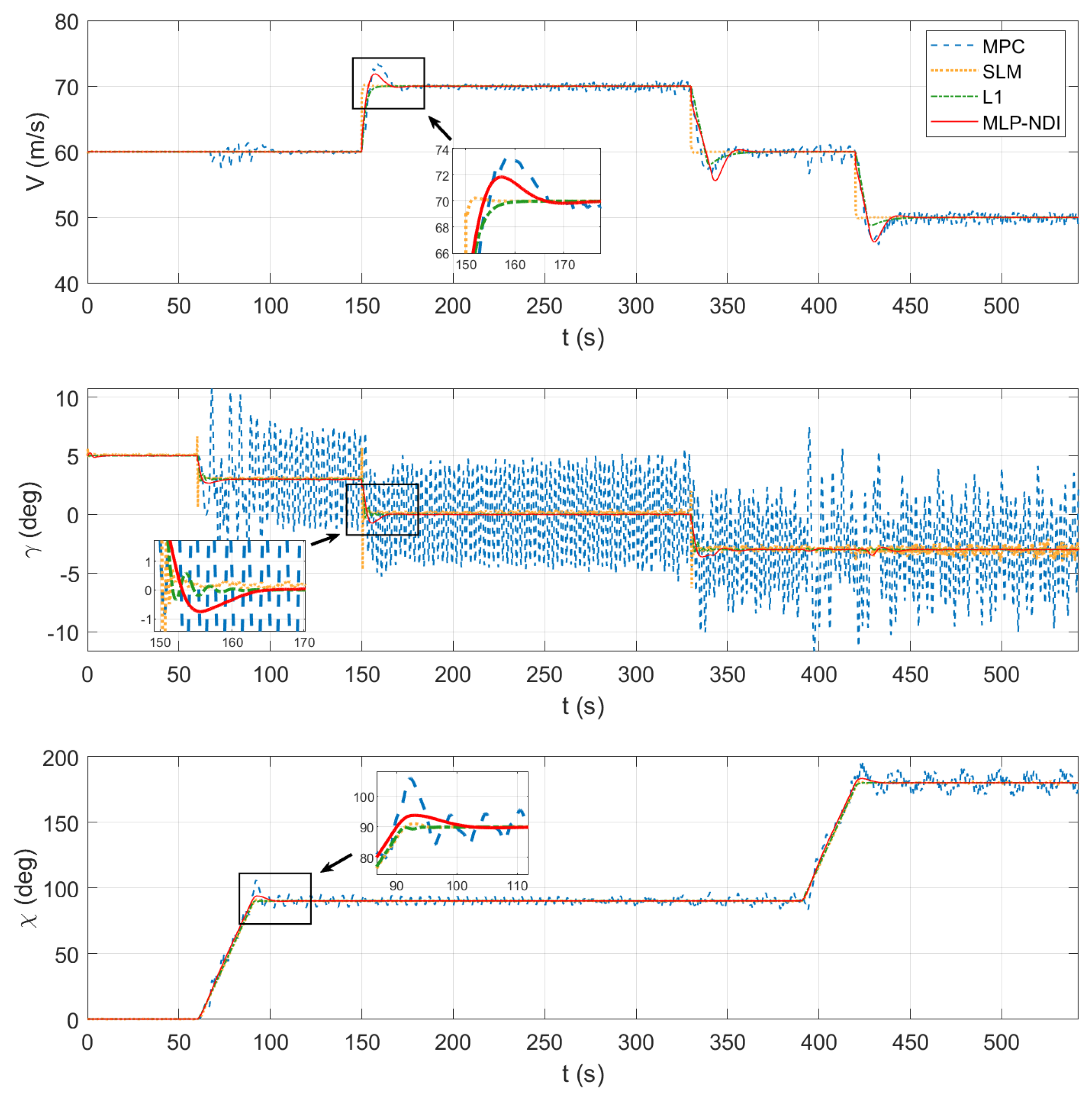
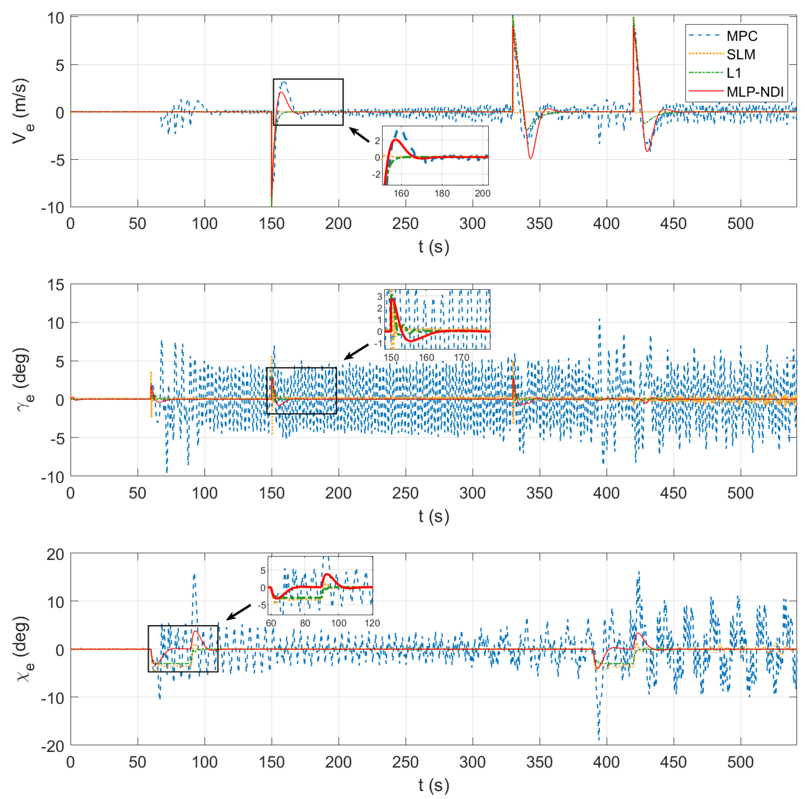
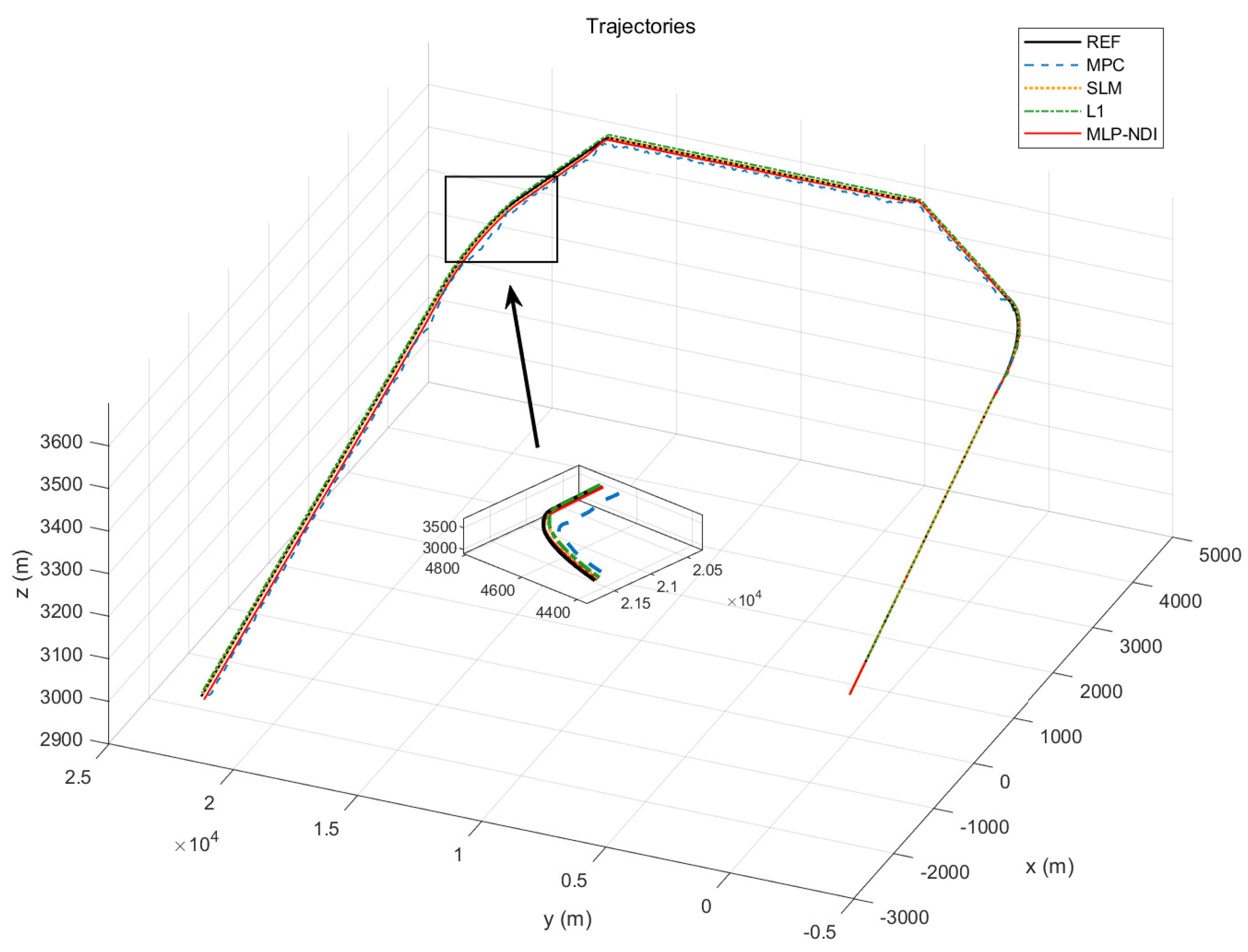
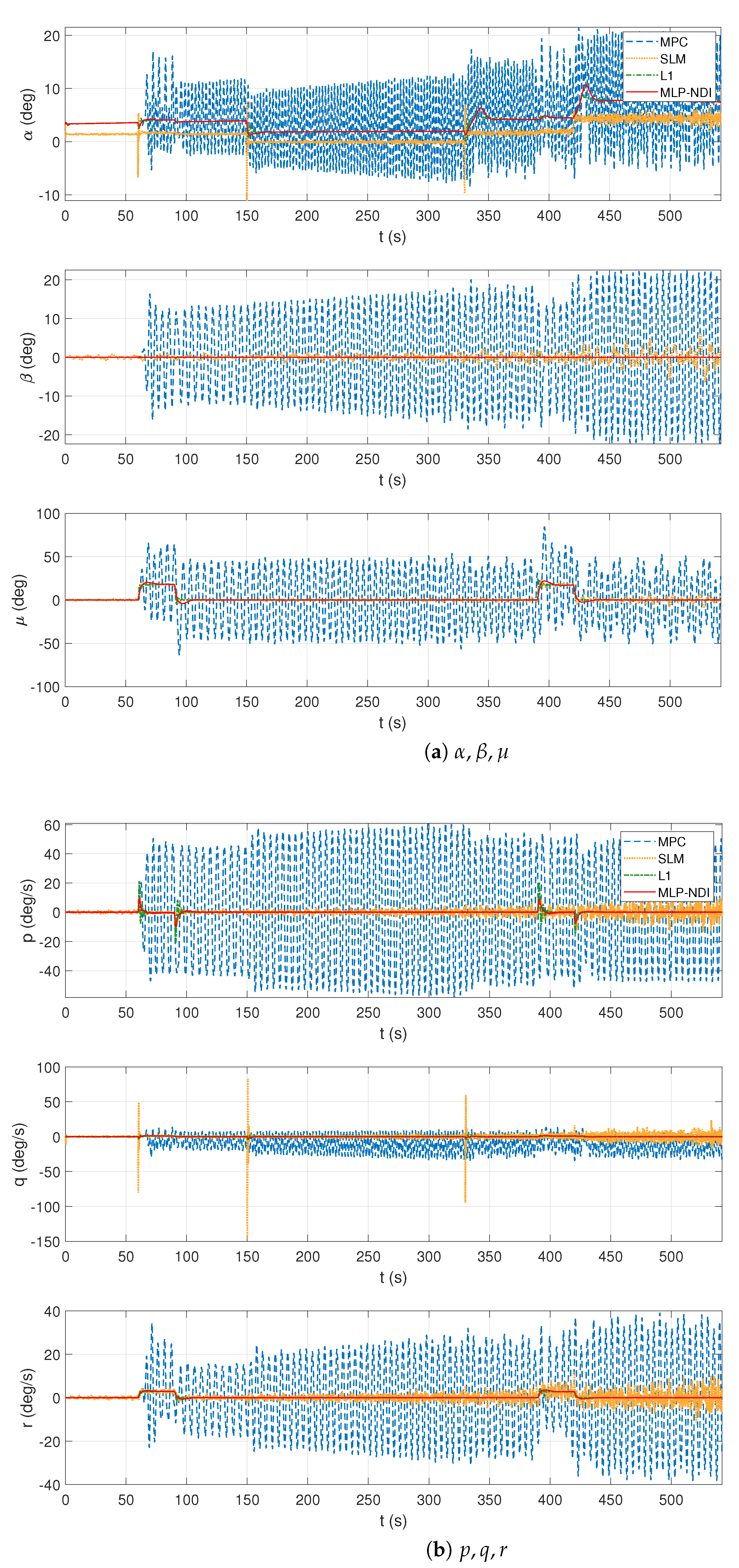
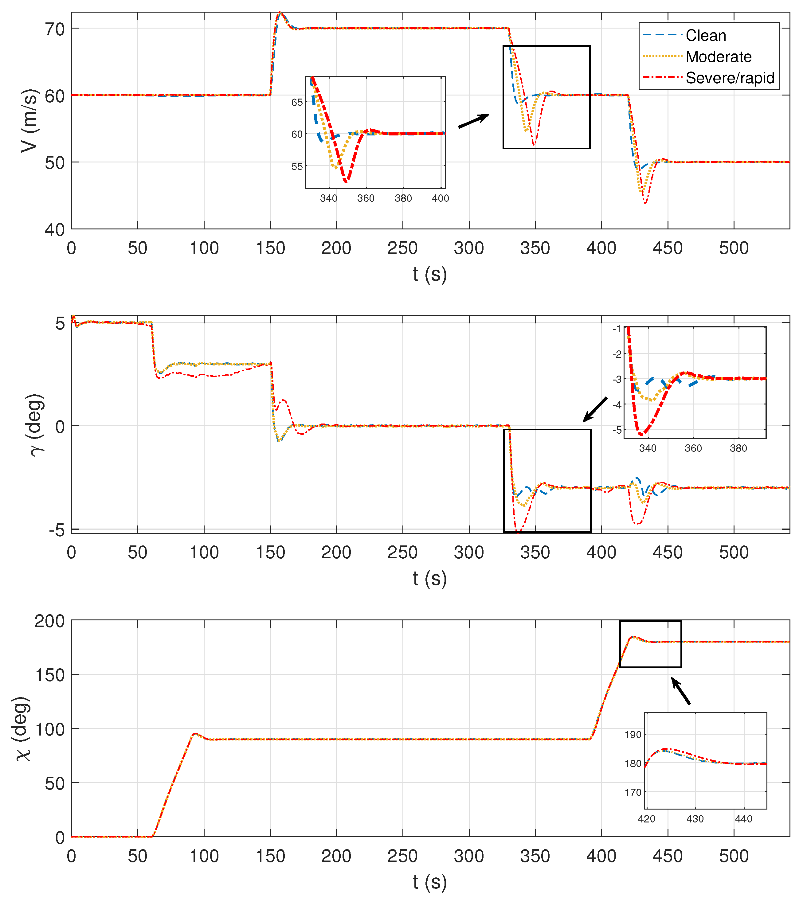
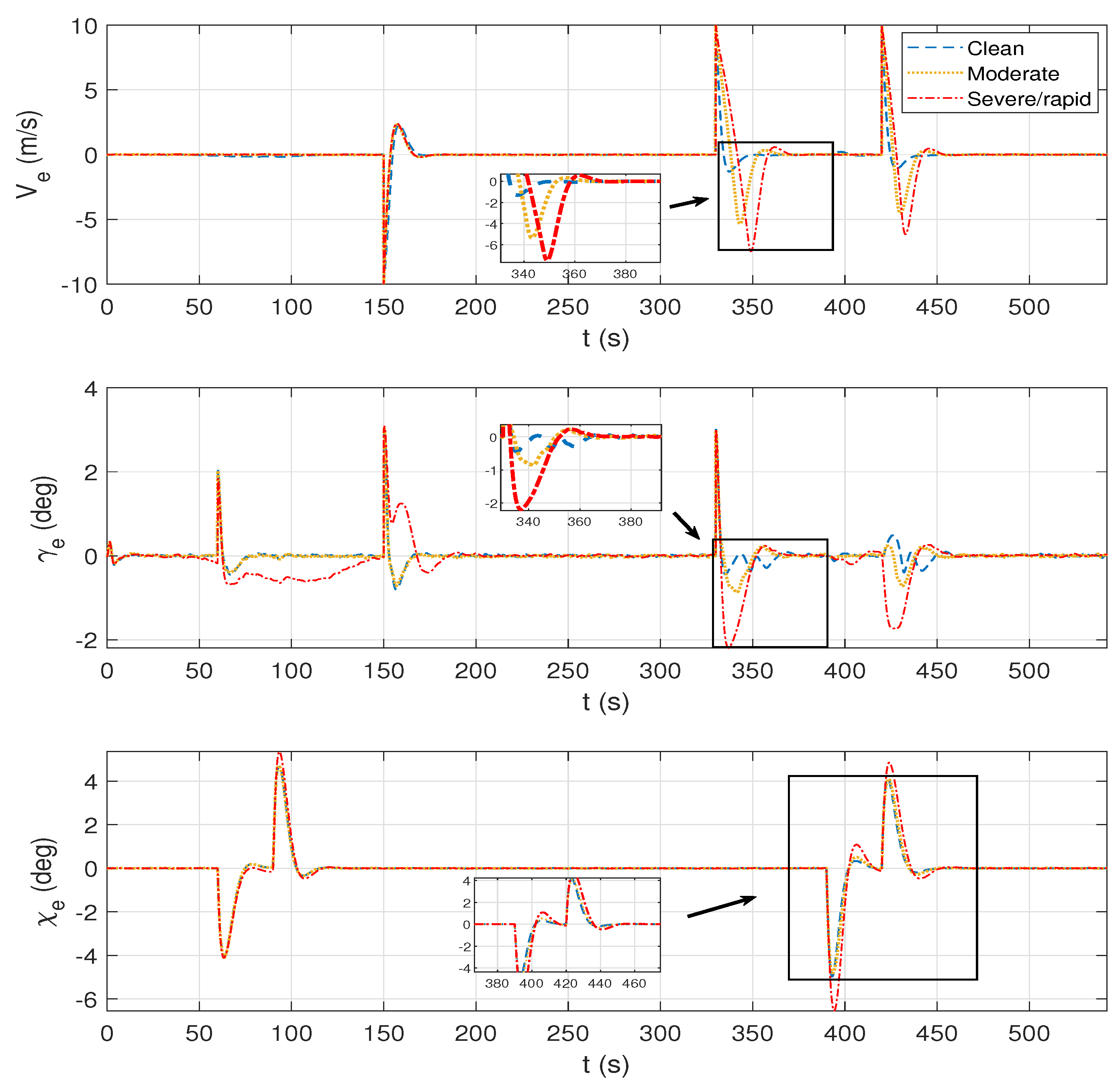
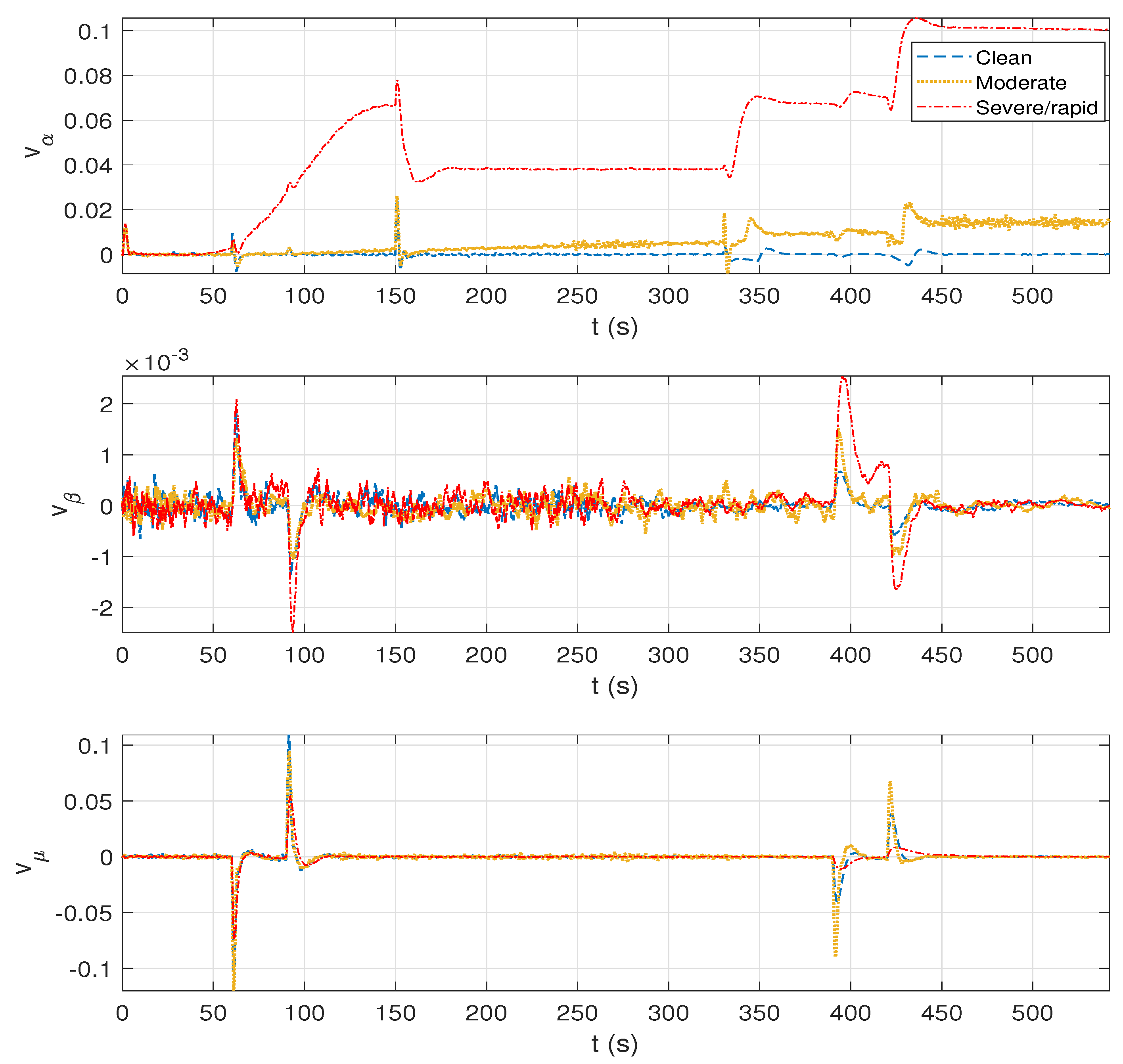
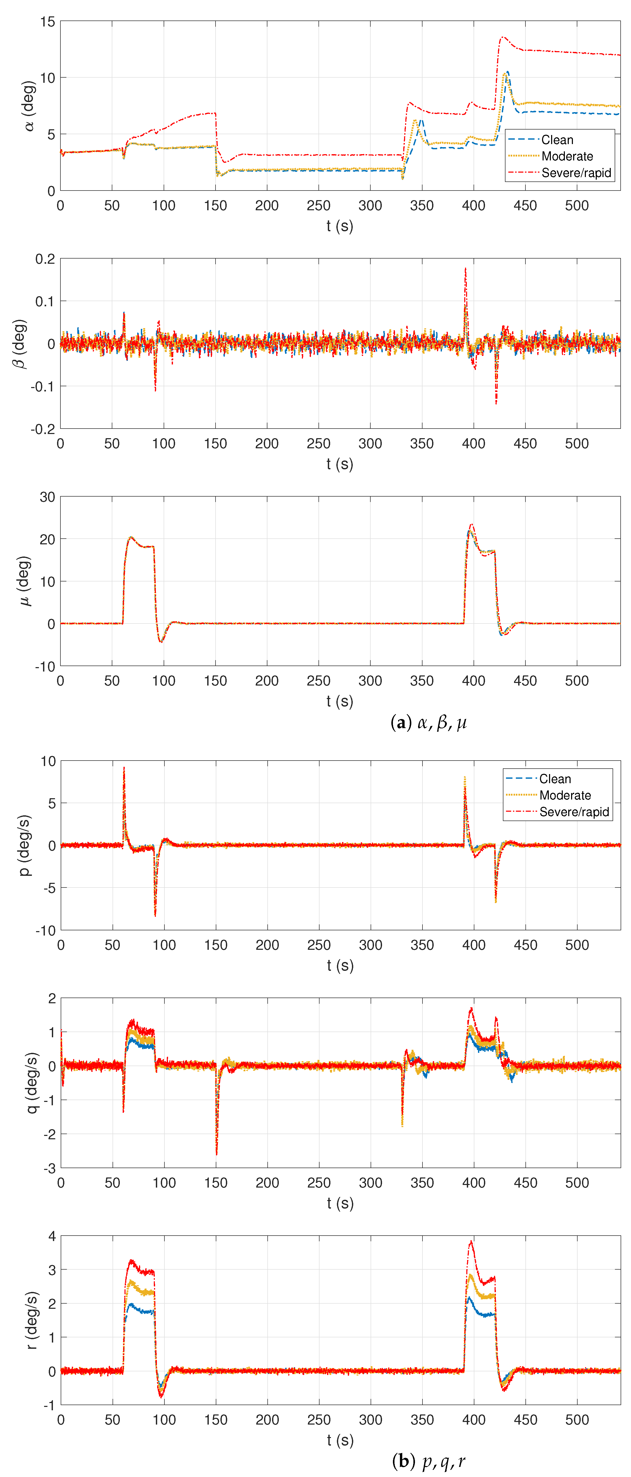
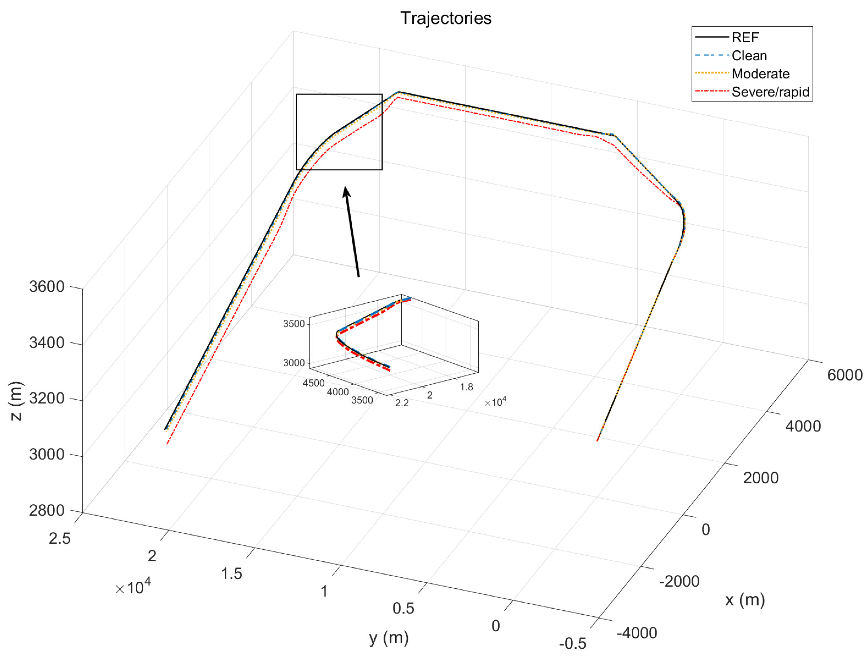
In this paper, a novel MLP-NDI controller was proposed and its performance in ice-tolerant control was demonstrated. To implement and test the controller, a DHC-6 model was constructed that includes icing effect, wind disturbance, and measurement noise. In addition to the MLP-NDI controller, three other controllers were also tested on this icing model, and the performance of all controllers was evaluated during various combined maneuvers.

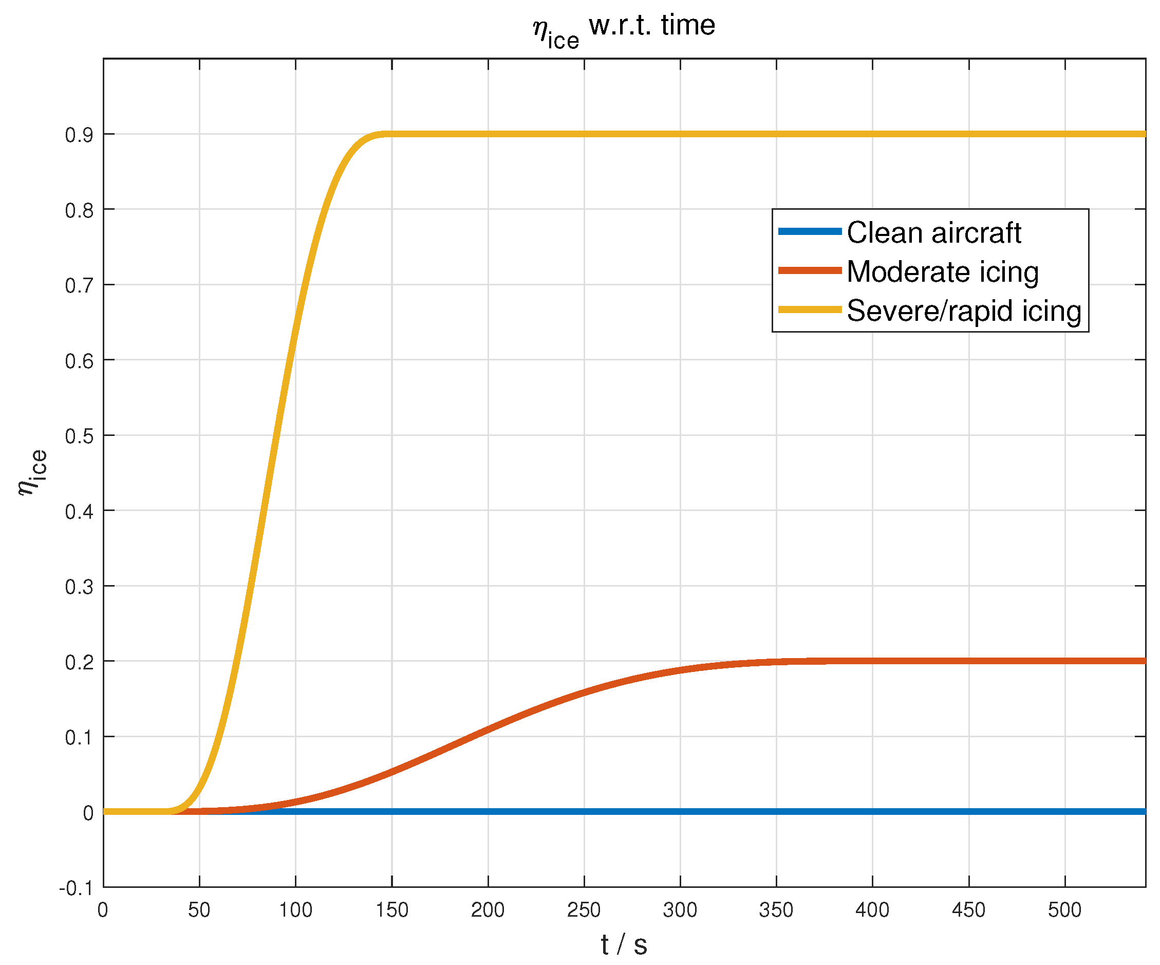
In the aforementioned modeling scenario, the traditional NDI method was found to have a huge inversion error brought by model uncertainty. To solve this problem, a compensator based on neural networks was designed for each of the three control channels. Two simulations were conducted with the following purposes: the first compared the MLP-NDI controller’s performance with other typical controllers, and the second tested its robustness under three icing scenarios. The results demonstrate that the MLP-NDI controller is capable of adapting to different icing conditions and exhibits strong robustness against in-flight icing.

Future work will involve the application of deep neural networks to the controller, and the consideration of more complex models, such as those involving center of gravity offset and shape asymmetry. In addition, the current controller will be tested and improved in more extreme conditions, including addressing actuator limitations or failures.

References

1. Bottyán, Z. Estimation of in-flight icing characteristics of UAVs during different meteorological conditions. In Proceedings of the 8th International Conference on Intelligent Unmanned Systems, Singapore, 22–24 October 2012; pp. 418–422. [Google Scholar]
2. Bragg, M. Aircraft aerodynamic effects due to large droplet ice accretions. In Proceedings of the 34th Aerospace Sciences Meeting and Exhibit, Reno, NV, USA, 15–18 January 1996; p. 932. [Google Scholar]
3. Cao, Y.; Wu, Z.; Su, Y.; Xu, Z. Aircraft flight characteristics in icing conditions. Prog. Aerosp. Sci. 2015, 74, 62–80. [Google Scholar] [CrossRef]
4. Melody, J.W.; Başar, T.; Perkins, W.R.; Voulgaris, P.G. Parameter identification for inflight detection and characterization of aircraft icing. Control Eng. Pract. 2000, 8, 985–1001. [Google Scholar] [CrossRef]
5. Dong, Y.; Ai, J. Inflight parameter identification and icing location detection of the aircraft: The time-varying case. J. Control Sci. Eng. 2014, 2014. [Google Scholar] [CrossRef]
6. Aircraft Accident Report, Inflight Icing Encounter and Loss of Control, ATR Model 72-212, Roselawn, Indiana, 31 October 1994; Tech. Rep. NTSB/AAR-96/01; National Transportation Safety Board: Washington, DC, USA, 1996.
7. Interim Report on the Accident on 1 June 2009 to the Airbus A330–203 Registered F-GZCP Operated by Air France Flight AF 447 Rio de Janeiro-Paris; Bureau d’Enquêtes et d’Analyses pour la Sécurité de l’Aviation Civile (BEA): Paris, France, 2009.
8. Safety Investigation Following the Accident on 1st June 2009 to the Airbus A330-203, Flight AF 447-Summary, English ed. Bureau d’Enquêtes et d’Analyses pour la sécurité de l’Aviation civile (BEA): Paris, France, 2012.
9. Ratvasky, T.; Van Zante, J.; Riley, J. NASA/FAA tailplane icing program overview. In Proceedings of the 37th Aerospace Sciences Meeting and Exhibit, Reno, NV, USA, 11–14 January 1999; p. 370. [Google Scholar]
10. Bragg, M.; Perkins, W.; Sarter, N.; Basar, T.; Voulgaris, P.; Gurbacki, H.; Melody, J.; McCray, S. An interdisciplinary approach to inflight aircraft icing safety. In Proceedings of the 36th AIAA Aerospace Sciences Meeting and Exhibit, Reno, NV, USA, 12–15 January 1998; p. 95. [Google Scholar]
11. Cheng, J.C.; Chen, Y.M. Investigation of fluid flow and heat transfer characteristics for a thermal anti-icing system of a high-altitude and long-endurance UAV. J. Mech. 2021, 37, 467–483. [Google Scholar] [CrossRef]
12. Muhammed, M.; Virk, M.S. Ice Accretion on Fixed-Wing Unmanned Aerial Vehicle—A Review Study. Drones 2022, 6, 86. [Google Scholar] [CrossRef]
13. Cao, Y.; Tan, W.; Wu, Z. Aircraft icing: An ongoing threat to aviation safety. Aerosp. Sci. Technol. 2018, 75, 353–385. [Google Scholar] [CrossRef]
14. Jiang, J.; Yu, X. Fault-tolerant control systems: A comparative study between active and passive approaches. Annu. Rev. Control 2012, 36, 60–72. [Google Scholar] [CrossRef]
15. Ding, D.; Che, J.; Qian, W.Q. Fault-tolerant flight control for aircraft wing icing based on icing detection method. In Proceedings of the 2018 IEEE CSAA Guidance, Navigation and Control Conference (CGNCC), Xiamen, China, 10–12 August 2018; pp. 1–6. [Google Scholar]
16. Ru, J.; Li, X.R. Variable-structure multiple-model approach to fault detection, identification, and estimation. IEEE Trans. Control Syst. Technol. 2008, 16, 1029–1038. [Google Scholar] [CrossRef]
17. Verhaegen, M.; Kanev, S.; Hallouzi, R.; Jones, C.; Maciejowski, J.; Smail, H. Fault tolerant flight control-a survey. In Fault Tolerant Flight Control; Springer: Berlin/Heidelberg, Germany, 2010; pp. 47–89. [Google Scholar]
18. Shtessel, Y.; Buffington, J.; Banda, S. Multiple timescale flight control using reconfigurable sliding modes. J. Guid. Control. Dyn. 1999, 22, 873–883. [Google Scholar] [CrossRef]
19. Mignone, D. Control and estimation of hybrid systems with mathematical optimization. Ph.D. Thesis, ETH Zurich, Zurich, Switzerland, 2002. [Google Scholar]
20. Funahashi, K.I. On the Approximate Realization of Continuous Mappings by Neural Networks. Neural Netw. 1989, 2, 183–192. [Google Scholar] [CrossRef]
21. Calise, A. Development of a reconfigurable flight control law for the X-36 tailless fighter aircraft. In Proceedings of the AIAA Guidance, Navigation, and Control Conference and Exhibit, Napoli, Italy, 13–16 June 2000; p. 3940. [Google Scholar]
22. Idan, M.; Johnson, M.; Calise, A.J.; Kaneshige, J. Intelligent aerodynamic/propulsion flight control for flight safety: A nonlinear adaptive approach. In Proceedings of the 2001 American Control Conference (Cat. No. 01CH37148), Arlington, VA, USA, 25–27 June 2001; Volume 4, pp. 2918–2923. [Google Scholar]
23. Hovakimyan, N.; Nardi, F.; Calise, A.; Kim, N. Adaptive output feedback control of uncertain nonlinear systems using single-hidden-layer neural networks. IEEE Trans. Neural Netw. 2002, 13, 1420–1431. [Google Scholar] [CrossRef] [PubMed]
24. Shin, D.H.; Kim, Y. Reconfigurable flight control system design using adaptive neural networks. IEEE Trans. Control Syst. Technol. 2004, 12, 87–100. [Google Scholar] [CrossRef]
25. Bragg, M.; Hutchison, T.; Merret, J. Effect of ice accretion on aircraft flight dynamics. In Proceedings of the 38th Aerospace Sciences Meeting and Exhibit, Reno, NV, USA, 10–13 January 2000; p. 360. [Google Scholar]
26. Ratvasky, T.; Ranaudo, R. Icing effects on aircraft stability and control determined from flight data-Preliminary results. In Proceedings of the 31st Aerospace Sciences Meeting, Reno, NV, USA, 11–14 January 1993; p. 398. [Google Scholar]
27. Melody, J.W.; Hillbrand, T.; Başar, T.; Perkins, W.R. H parameter identification for inflight detection of aircraft icing: The time-varying case. Control Eng. Pract. 2001, 9, 1327–1335. [Google Scholar] [CrossRef]
28. Dong, Y.; Ai, J. Research on inflight parameter identification and icing location detection of the aircraft. Aerosp. Sci. Technol. 2013, 29, 305–312. [Google Scholar] [CrossRef]
29. Fang, Z.; Chen, W.; Zhang, S. Aerospace Vehicle Dynamics, 1st ed.; Beihang University Press: Beijing, China, 2005. [Google Scholar]
30. Pokhariyal, D.; Bragg, M.; Hutchison, T.; Merret, J. Aircraft flight dynamics with simulated ice accretion. In Proceedings of the 39th Aerospace Sciences Meeting and Exhibit, Reno, NV, USA, 8–11 January 2001; p. 541. [Google Scholar]
31. Lewis, F.L.; Yesildirek, A.; Liu, K. Multilayer neural-net robot controller with guaranteed tracking performance. IEEE Trans. Neural Netw. 1996, 7, 388–399. [Google Scholar] [CrossRef]
32. Snell, S.A.; Enns, D.F.; Garrard, W.L., Jr. Nonlinear inversion flight control for a supermaneuverable aircraft. J. Guid. Control. Dyn. 1992, 15, 976–984. [Google Scholar] [CrossRef]
33. Wang, L. Model Predictive Control System Design and Implementation Using MATLAB®; Springer Science & Business Media: Berlin/Heidelberg, Germany, 2009. [Google Scholar]
34. Jafarov, E.M.; Tasaltin, R. Robust sliding-mode control for the uncertain MIMO aircraft model F-18. IEEE Trans. Aerosp. Electron. Syst. 2000, 36, 1127–1141. [Google Scholar]
35. Wang, T.; Xie, W.; Zhang, Y. Adaptive sliding mode fault tolerant control of civil aircraft with separated uncertainties. In Proceedings of the 48th AIAA Aerospace Sciences Meeting Including the New Horizons Forum and Aerospace Exposition, Orlando, FL, USA, 4–7 January 2010; p. 945. [Google Scholar]
36. Pu, M.; Wu, Q.; Jiang, C.; Dian, S.; Wang, Y. Recursive terminal sliding mode control for higher-order nonlinear system with mismatched uncertainties. Acta Autom. Sin. 2012, 38, 1777–1793. [Google Scholar] [CrossRef]
37. Hovakimyan, N.; Cao, C. L1 Adaptive Control Theory: Guaranteed Robustness with Fast Adaptation; SIAM: Urbana, IL, USA, 2010. [Google Scholar]
38. Banerjee, S.; Boyce, R.; Wang, Z.; Baur, B.; Holzapfel, F. L1 augmented controller for a lateral/directional maneuver of a hypersonic glider. J. Aircr. 2017, 54, 1257–1267. [Google Scholar] [CrossRef]
39. Chen, Q.; Wan, J.; Ai, J. L 1 adaptive control of a generic hypersonic vehicle model with a blended pneumatic and thrust vectoring control strategy. Sci. China Inf. Sci. 2017, 60, 32203. [Google Scholar] [CrossRef]
40. Levant, A. Sliding order and sliding accuracy in sliding mode control. Int. J. Control 1993, 58, 1247–1263. [Google Scholar] [CrossRef]
41. Hellmundt, F.; Wildschek, A.; Maier, R.; Osterhuber, R.; Holzapfel, F. Comparison of L1 adaptive augmentation strategies for a differential PI baseline controller on a longitudinal F16 aircraft model. In Advances in Aerospace Guidance, Navigation and Control; Springer: Berlin/Heidelberg, Germany, 2015; pp. 99–118. [Google Scholar]
Figure 1. Nonlinear adaptive output feedback controller.
Drones 07 00273 g001
Figure 2. NASA Glenn Research Center icing research aircraft (DHC-6) https://www1.grc.nasa.gov/facilities/hangar/ (accessed on 1 March 2023).
Drones 07 00273 g002
Figure 3. Icing severity for the clean and two icing cases.
Drones 07 00273 g003
Figure 4. Structure of MLP-NDI controller.
Drones 07 00273 g004
Figure 5. MLP compensator.
Drones 07 00273 g005
Figure 6. The overall control architecture DHC-6.
Drones 07 00273 g006
Figure 7. Structure of MLP-NDI in slow attitude system.
Drones 07 00273 g007
Figure 8. Structure of MLP-NDI in fast rotational system.
Drones 07 00273 g008
Figure 9. Signal tracking of V, γ , and χ .
Drones 07 00273 g009
Figure 10. Tracking error of V, γ , and χ .
Drones 07 00273 g010
Figure 11. Overall trajectories of 4 controllers.
Drones 07 00273 g011
Figure 12. Inner-loop states of different controllers.
Drones 07 00273 g012
Figure 13. Signal tracking of V, γ , and χ .
Drones 07 00273 g013
Figure 14. Tracking error of V, γ , and χ .
Drones 07 00273 g014
Figure 15. MLP compensation of v α , v β , v μ .
Drones 07 00273 g015
Figure 16. Inner-loop states under three icing scenarios.
Drones 07 00273 g016
Figure 17. Overall flight trajectories under three icing scenarios.
Drones 07 00273 g017