Article

Transition Nonlinear Blended Aerodynamic Modeling and Anti-Harmonic Disturbance Robust Control of Fixed-Wing Tiltrotor UAV

Department of Aerospace Engineering, Korea Advanced Institute of Science and Technology, Daejeon 34141, Republic of Korea
*
Author to whom correspondence should be addressed.
Drones 2023, 7(4), 255; https://doi.org/10.3390/drones7040255
Submission received: 8 March 2023 / Revised: 4 April 2023 / Accepted: 5 April 2023 / Published: 10 April 2023
(This article belongs to the Special Issue Flight Control System Simulation)

Abstract

:
This study proposed a novel nonlinear blended aerodynamic model for the tiltrotor unmanned aerial vehicle (UAV) during the transition phase to handle the high angle-of-attack (AoA) flight, which aggregated the flat-plate mode and the linear mode of the aerodynamic coefficients. Additionally, a harmonic disturbance observer (HDO) and super-twisting sliding mode controller (STSMC) addressed the fast-changing external disturbances and attenuated the chattering problem in the original SMC. The comparative trajectory tracking results indicated that the blended aerodynamic model accurately tracks the reference signals with no tracking errors, which demonstrated a superior performance as compared to the traditional aerodynamic model, with a reduction of 2.2%, 50%, 73.6%, and 11.2% in the time required for tracking the pitch angle, pitch rate, and velocities u and w, respectively. Conversely, the traditional one exhibited significant tracking errors, ranging from 0.016° in the pitch angle channel to 1.25°/s in the pitch rate channel, and 0.6 m/s for velocity u and 0.01 m/s for velocity w. Moreover, the comparative control input results illustrated that the least control effort was required for the proposed HDO-STSMC control scheme with a blending function, while the original ESO-SMC experienced more oscillations and sharp amplitude changes, taking twice the time to converge, with considerable tracking errors such as 1.067° in the pitch angle channel, 0.788°/s in the pitch rate channel, 1.554 m/s for velocity u, and 0.746 m/s for velocity w, which verified the feasibility and superiority of the proposed HDO-STSMC with the blending function. Two performance indices revealed the robust stability and rapid convergence of the proposed transition blended aerodynamic model with the HDO-STSMC control scheme.

1. Introduction

Combining traditional aircraft with tiltable quadrotors enables the convertible unmanned aerial vehicle (UAV) to have a high forward-flight speed and tolerance. One of the well-known advantages of the convertible quadrotor UAV is its vertical take-off and landing (VTOL), which also leads to high demands on the control system during the transition phase, mainly referring to the phase between the hovering phase and the forward-flight phase, and vice versa.
Regarding the modeling of the transition phase, one of the most heated research topics is the calculation of the aerodynamics of the fixed wing. Many researchers have tried to model the aerodynamic interference between the fixed wing and rotors mathematically to achieve further accuracy in fixed-wing aerodynamics. For example, Flores et al. took the airflow speed produced by the rotors into consideration and roughly weighted the aerodynamic effects of the rotor-induced airflow acting on the wings as 1 and 0 [1], while Yuksek et al. proposed an effectiveness coefficient that was modeled as a sigmoid function with respect to the tilt angle; the calculation of the area that was affected by the rotor-induced airflow was also presented [2]. A sophisticated derivation in the uncertain forces generated by the rotors and exerted on the fixed wing was presented, based on the blade element method in reference [3]. However, the key weakness of the linear aerodynamic model of the fixed wing is that it fails to predict the abrupt drop in the lift force with an increasing angle of attack (AoA), which is caused by the turbulent flow and is taken into consideration for the designs, such as the tiltwing [4] and the aerodynamically similar tailsitter [5,6,7]. What is worse is that the mainstream method of modeling the aerodynamic coefficients of the fixed-wing tiltrotor UAV is derived based on the low AoA [3,8,9,10,11,12]. At the same time, the high AoA aerodynamics modeling approach is often costly and requires wind tunnel experiments [13,14], from which smooth fits of aerodynamic coefficient data will be produced through cubic spline interpolation. The main reason why high AoA aerodynamics modeling matters is that the AoA will be larger than the stall angle when the UAV enters the transition phase; for that, high AoA aerodynamics should be considered. One of the inspiring full-envelope aerodynamics mathematical modeling approaches, the 2D-to-3D correction method, was proposed in reference [15], which successfully predicted the local airfoil section data at a high angle with large control deflections. This correction method was also introduced in reference [16], which presented satisfactory tracking results of the corrected signals with moderate control effort compared with the original pilot input signals. Another more straightforward approach is designing a blending function, which is used to incorporate the wing stall into the full-envelope aerodynamic model so that the aerodynamic forces and moments are modeled nonlinearly in the AoA, ranging from π to π . Reference [17] used the hyperbolic tangent t a n h blending function to aggregate the low AoA aerodynamic model and the high AoA aerodynamic model together, while references [18,19,20] proposed a sigmoid function as the blending function, and the blended lift, drag, and pitching moment coefficients were provided in an organized form. However, none of the previous research on designing the proper blending functions compared the blended full-envelope flight results with the one generated by the traditional aerodynamic model. Hence, the first main contribution of this paper is to design the proper blending function for aggregating the low AoA model and the flat-plate model together, and then compare the trajectory tracking performance with the one generated by the non-blended aerodynamic model.
In the flight control scheme, combining the sliding mode control (SMC)-based algorithm and various kinds of disturbance observers is gradually becoming a popular and effective way to handle modeling uncertainties and external disturbances. Typically, in the multirotor UAV with passively canted or actuated rotors, known as a non-planar multirotor UAV, SMC is widely used to deal with modeling uncertainties because of its well-known strong robustness [
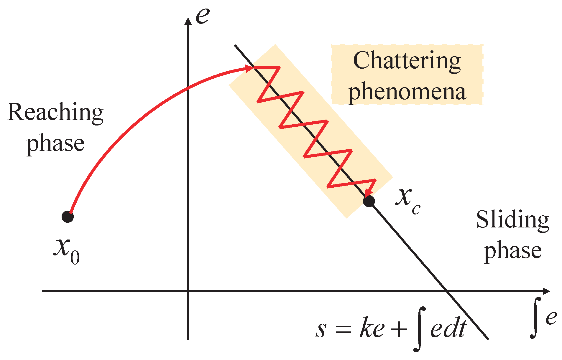
21]. To alleviate the chattering problems caused by the time delays in the switching control law [22], second- and higher-order SMC has been developed to overcome this while maintaining the finite-time convergence to the sliding surface. The super-twisting algorithm (STA) is one of the most popular second-order sliding mode techniques, developed by Levant [23] and further generalized by Haimovich and De Battista, which is taken as a powerful technology to handle the undesirable chattering phenomenon caused by the switching of the discontinuous control laws from one to another. Regarding handling external disturbances, the extended state observer (ESO), which stems from the active disturbance rejection control (ADRC), is also famous for its stability and feasibility. As one of the time-domain disturbance observers, the ESO extends an extra state for the estimated disturbance, as the system states; then, a disturbance observer is developed to estimate the additional disturbance states [24]. Compared with the traditional SMC and ESO, STA-based controllers/disturbance observers are more widely used for systems with uncertainties for which the boundary is assumed to be known. For example, reference [25] proposed SMC and a finite-time super-twisting extended state observer (STESO) to handle the total disturbances in the novel proposed integrated guidance and control scheme of the skid-to-turn interceptor, and the closed-loop stability was guaranteed based on the Lyapunov theory. A continuous super-twisting controller combined with a high-order sliding mode (HOSM) observer was presented in reference [26] to address a class of uncertain nonlinear systems, and the feasibility of the proposed controller–observer scheme for UAV altitude control was verified via numerical simulations and experimental tests. The STESO was also presented to estimate the lumped disturbances, which can avoid stimulating the sensor noise caused by the higher-order ESO. Super-twisting SMC (STSMC) was developed to ensure the accuracy of trajectory tracking [27]. Reference [28] proved that the STESO can estimate disturbances faster than the original ESO. The wind gust and actuator faults can be handled by designing the STESO and SMC control structure [29]. The previous research shows that introducing the STA can enhance the control performance compared with the original SMC and ESO.
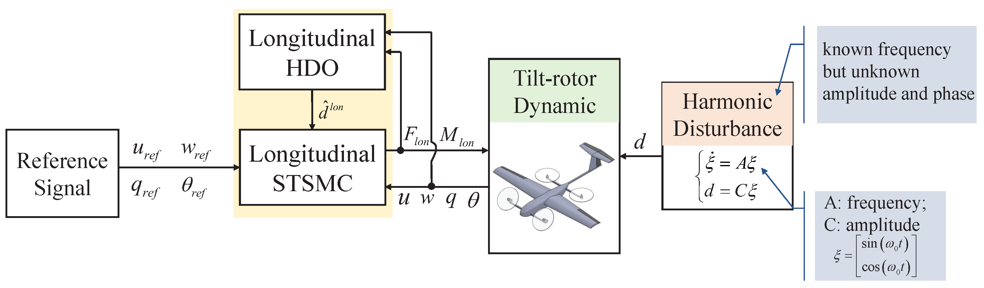
However, the external disturbances that exist in the aircraft with the wind shear are often modeled as harmonic with a known frequency but unknown amplitude and phase [30], while the original ESO is designed to handle the slow-changing disturbances instead of the periodic ones [31]. Accordingly, the harmonic disturbance observer (HDO) [32] was introduced to the flight control system to deal with the external harmonic disturbances. The main advantage of applying an HDO to handle harmonic disturbances is that an HDO is designed to handle periodic disturbances specifically. Many pieces of research have proved its stability with the Lyapunov theory and the feasibility with the simulation. Reference [33] presented the proposed nonlinear HDO, which guaranteed the stability of the closed-loop system consisting of the nonlinear disturbance observer and a traditional controller that stabilized the nonlinear system without disturbances. The well-designed HDO was integrated with the computed torque controller for the two-link robotic manipulator. The simulation results indicated that the performance of the controller with the disturbance was significantly improved, and the HDO had a great disturbance attenuation ability [34]. The HDO in [35], combined with the proposed PID-STSMC, estimated the exogenous disturbance to realize the excellent tracking performance and superior stability of UAV attitude and altitude control without obvious chattering problems. Moreover, an HDO was introduced in the high-dynamic permanent magnet synchronous motor (PMSM) to suppress the harmonic disturbances with a high frequency in reference [36]. However, all the previous research did not prove the outperformance of the HDO compared with other kinds of disturbance observers. Hence, another main contribution of this paper is by introducing the HDO into the flight control scheme to estimate the external disturbances and design the STSMC control laws to compensate for the estimated disturbances without obvious chattering problems, comparing the trajectory tracking results generated by the HDO-STSMC with the ones generated by the original ESO-SMC, to achieve the goal of emphasizing the outperformance of the HDO dealing with the periodic external disturbances compared with the other kinds of disturbance observers.
Based on the above analysis, the main contributions of this paper can be summarized as follows:
(1)
The longitudinal aerodynamic model introduces a nonlinear blending function to guarantee a smooth transition phase when the UAV experiences a high AoA. A blended model of the forces/moments versus the AoA for the fixed-wing design over an extensive range of AoAs can be obtained without costly wind tunnel testing or a detailed computational study. The comparative simulation results between the blended aerodynamic model and the original aerodynamic model will be illustrated to verify the outperformance and feasibility of the blended aerodynamic model.
(2)
The STA is introduced to handle the chattering problems in the original SMC, designed to handle the model uncertainty with robustness. By integrating the discontinuous sign function, the chattering phenomenon caused by the discontinuous term can be attenuated by the STA without losing the robustness and accuracy of the STSMC.
(3)
A nonlinear HDO is integrated with the STSMC for the nonlinear dynamic system during the transition phase to handle the bounded harmonic disturbances so that the disturbance rejection ability of the flight control system can be enhanced. The comparative simulation results between the HDO-STSMC and the original ESO-SMC will be illustrated to emphasize the outperformance of the HDO dealing with periodic external disturbances compared with the other kinds of disturbance observers.
(4)
The closed-loop stability analysis of the HDO-STSMC control scheme is provided by the Lyapunov theory, where sufficient conditions are presented to guarantee convergence and select the suitable gains of the proposed controller.
The remainder of this paper is arranged as follows. Section 2 presents a mathematical model of the transition phase; the nonlinear blending function is introduced to blend the low AoA and flat-plate aerodynamic models together to handle the high AoA flight situation, which is beyond the scope of the traditional aerodynamic model. Then, the HDO-STSMC control scheme is presented in Section 3, as well as the stable conditions of the individual controllers and observers, which are derived based on the analysis of the Lyapunov theory. In Section 4, the global exponential stability of the closed-loop system under the nonlinear HDO-STSMC-based longitudinal autopilot is proved based on the Lyapunov theory. In Section 5, the comparative simulation results are presented for both the blended aerodynamic model and the original one, as well as for the proposed HDO-STSMC and the original ESO-SMC. Finally, the conclusions are presented in Section 6.

2. Mathematical Model with the Nonlinear Blending Function of the Transition Phase

In this section, the mathematical model with the nonlinear blending function of the transition phase is presented. A nonlinear blending function is introduced to handle the dramatic changes in aerodynamic coefficients around the stall angles of the fixed wing. Therefore, instead of linearly modeling the aerodynamic coefficients versus the AoA, a force/moment model that incorporates the common linear behavior and the effects of the stall is provided in this section.
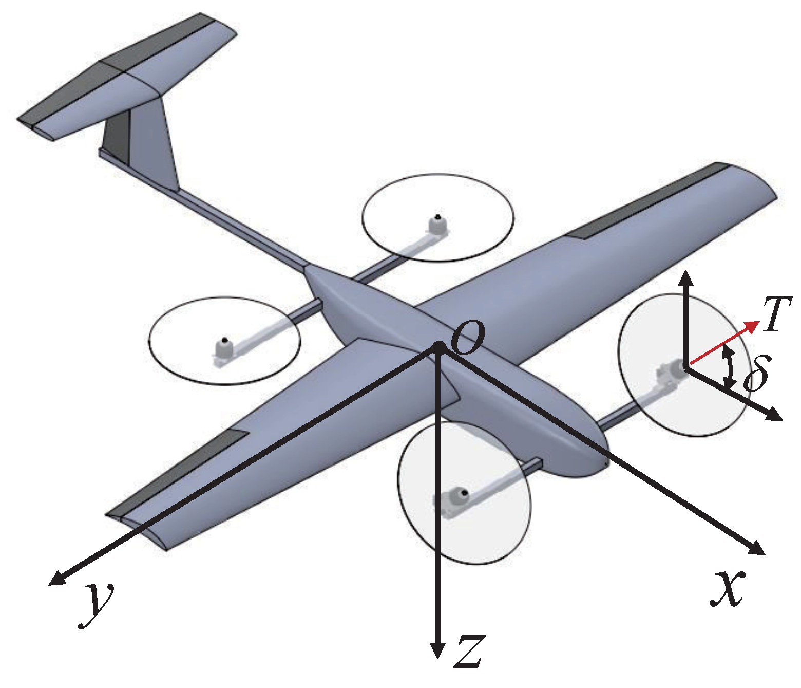
Hypothesis 1 (H1). 
The UAV is symmetric about the o x z plane and the mass is uniformly distributed.
The quad tiltrotor UAV configuration [37] and the generalized body-fixed frame o x y z with the origin o coincident with the center of gravity c g is presented in Figure 1.
The generalized longitudinal aerodynamics of the UAV can be described as Equation (1).
m u ˙ + q w = L a + Z g + Z r m w ˙ q u = D a + X g + X r I y q ˙ = M a + M g + M r
where the subscripts a, g, and r represent the aerodynamic, gravitational, and rotor dynamic terms, respectively; ( u , w ) represent the components of velocity along the axes o x and o z , respectively; q represents the component of angular velocity along the axes o y ; L a and D a represent the aerodynamic lift and drag along the axes o x and o z , respectively; Z g and X g represent the gravitational lift and drag along the axes o x and o z , respectively; Z r and X r represent the rotor-related lift and drag along the axes o x and o z , respectively; M i ( i = a , g , r ) represent the pitching moments along the o y axis.
The goal of modeling the aerodynamics that act on the fixed wing during the transition phase is to obtain a reasonable and accurate mapping from the UAV states to control aerodynamic variables within the flight-operating envelope [38]. The longitudinal aerodynamics can be described in detail as follows.
L a = 1 2 ρ V a 2 S C L ( α ) D a = 1 2 ρ V a 2 S C D ( α ) M a = 1 2 ρ V a 2 S c ¯ C M ( α )
where ρ = 1.2133 kg / m 3 is the air density at the altitude of operation which is 100 m above sea level in this study, V a = u 2 + w 2 is the airspeed of the UAV, S = 0.550 m 2 is the fixed-wing projected area, b = 2 m is the wing span, and c ¯ = 0.282 m is the mean aerodynamic chord; α denotes the angle of attack (AoA), which is defined as follows.
α = tan 1 w u = atan 2 w , u = θ γ , α π , π
where γ stands for the flight path angle.
During the transition phase, the AoA ( α ) in Equation (3) cannot be assumed to be small, because the flight path angle γ could be large. Meanwhile, the aerodynamic coefficients listed in Equation (2) drastically change at the stall angles α s , which can be described as follows when these coefficients are modeled based on the case of the flat plate [18,19].
C L , flat plate ( α ) = 2 sign ( α ) sin 2 α cos α C D , flat plate ( α ) = sin 2 ( α ) C M , flat plate ( α ) = sign ( α ) sin ( α ) sin ( α / 2 )
When the AoA α is smaller than the stall angle α s , the aerodynamic coefficients are modeled as in the following equations.
C L , low AoA ( α ) = C L 0 + C L α α C D , low AoA ( α ) = C D 0 + C D α 1 α + C D α 2 α 2 C M , low AoA ( α ) = C M 0 + C M α α
The aerodynamic parameter values for Equation (5) are listed in Table 1 [37].
To continuously blend these two models, the aerodynamic coefficients are assumed to be represented for π α π by the following equation.
C ( α ) = [ 1 σ ( α ) ] C , low AoA ( α ) + a 1 [ σ ( α ) σ ( α π ) σ ( α + π ) ] C , flat plate ( α ) + a 2 [ 1 σ ( α π ) ] C , low AoA ( α ) + a 3 [ 1 σ ( α + π ) ] C , low AoA ( α )
where ∗ represents the lift (L), drag (D), and pitching moment (M), and the blending function σ ( α ) is defined as follows.
σ ( α ) = 1 + e R α α s + e R α + α s 1 + e R α α s 1 + e R α + α s
where R represents the transition rate and α s represents the stall angle. The parameters a i ( i = 1 , 2 , 3 ) of Equation (6) [19], and transition rate R, stall angle α s are given in Table 2.
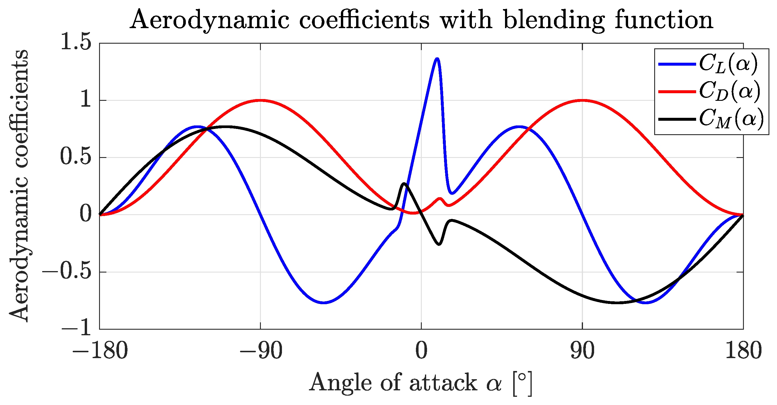
The aerodynamic coefficients C L α , C D α , and C M α of NACA9412, calculated by Equation (6), are illustrated in Figure 2, from which one can tell the nonlinear blending function aggregates low AoA and high AoA aerodynamic model together successfully.
Because the origin of the body-fixed frame o defined above coincides with the center of gravity c g , there are no gravitational moments about the axis: M g = 0 . The gravitational lift and drag along o x and o z axes can be expressed as follows.
Z g X g = sin θ cos θ cos ϕ m g
where ϕ and θ are the Euler angles defined according to the o x and o y axes, respectively.
By tilting the quadrotors from 90° (the VTOL phase) to 0° (the forward-flight phase) with tilt angle δ , the UAV enters the transition phase. The pitching moments M r i ( i = 1 , 2 , 3 , 4 ) of each rotor in the quadrotor system concerning the body-fixed frame can be modeled as follows.
M r i = o o r i × T i = r i x cos δ r i z sin δ k T ω i 2 , i = 1 , 2 , 3 , 4
where T i i = 1 , 2 , 3 , 4 = k T ω i 2 are the thrusts generated by the quadrotors, coefficient k T can be determined via the static thrust tests, and o o r i = r i x r i z T i = 1 , 2 , 3 , 4 denotes the positions of four rotors concerning the center of gravity o, which is presented in Table 3 [37].
Then, the total pitching moments generated by the rotor system can be expressed as follows.
M r = i = 1 4 M r i
Meanwhile, the forces generated by the rotor system during the transition phase can be described as follows.
Z r X r = k T sin δ k T cos δ i = 1 4 ω i 2
Based on the above analysis, the longitudinal equations of motion describing the changes in the axial and normal velocities u and w, pitch rate and angle q and θ , position range x, and altitude z of UAV transition phase can be presented as follows.
u ˙ = q w + F x m w ˙ = q u F z m q ˙ = 1 I y M x ˙ = u cos θ + w sin θ z ˙ = u sin θ + w cos θ θ ˙ = q
where forces F x = L a + Z g + Z r and F z = D a + X g + X r represent the summation of the forces generated by the aerodynamic ( L a and D a ), gravitational ( Z g and X g ), and rotors system ( Z r and X r ) analyzed above along with the o x and o z axes, respectively; the pitching moment M = M a + M r represents the summation of the moments generated by the aerodynamic ( M a ) and rotors system ( M r ) analyzed above, along with the o y axis.
The UAV parameters are presented in Table 4.

3. Harmonic Disturbance Observer-Based Super-Twisting Sliding Mode Control Scheme Design

Historically, SMC stems from the variable structure system (VSS), which is insensitive to certain external disturbances and model uncertainties, as well as robustness to parasitic dynamics. The core idea of SMC is to steer the trajectory of the nonlinear system to the properly chosen sliding manifold (or the sliding surface), and then maintain motion on the manifold thereafter by means of the control [39]. The graphical interpretation of the basic SMC is presented in Figure 3.
This section proposes a robust control structure that can perform effectively against the model uncertainties and external disturbances, based on the combination of STSMC and HDO, which are used to handle the uncertainties/disturbances that negatively influence the UAV tracking performance. The flight control scheme will be designed in two steps: firstly, STSMC is designed for the nominal plant modeled above to achieve stability and tracking performance without considering the disturbance, uncertainties, and unmodeled dynamics; then, HDO is designed to compensate for these ignored internal and external disturbances, and to realize the disturbance attenuation and robustness. The overview of the nonlinear HDO-STSMC control scheme is presented in Figure 4.

3.1. Super-Twisting Sliding Mode Control Law Design

As a widely used second-order SMC, the main characteristic of STSMC is that the majorant trajectory of the sliding mode manifold s and its derivative rotates, twisting around the origin in the phase plane. The STSMC can guarantee that the manifolds designed for the longitudinal channels s = ( s θ , s q , s u , s w ) converge to zero in finite time for the system with unknown bounded disturbances. The expression of the super-twisting switching control law in STSMC is defined as follows.
U sw = k 1 s 1 2 s i g n s + Q Q ˙ = k 2 s i g n s
where k 1 and k 2 are the control gains that must be properly determined. The switching control law U sw is designed to handle internal disturbances and mitigate the chattering problems without affecting the robustness. The integration of the discontinuous control variant function s i g n s reveals a better anti-chattering potential than the first-order SMC, mathematically.
Moreover, assuming the unknown bounded disturbances d t that will be estimated by the HDO and compensated by the STSMC satisfy d t d , the notable breakthrough in determining the control gains was achieved in reference [40], based on the Lyapunov functions yielding sufficient conditions for finite-time stability in the system.
k 2 > d k 1 > 2 k 2 k 2 2 d 2
The assumptions used to simplify the longitudinal decoupled model are listed as follows:
Hypothesis 2 (H2). 
Assumed to be a wing-level flight with zero sideslip, ϕ is small enough to obtain cos ϕ 1 and sin ϕ 0 .
Hypothesis 3 (H3). 
f x lon , g 1 x lon , and g 2 x lon are smooth functions and differentiable.
Therefore, the decoupled longitudinal dynamics can be written as follows.
x ˙ lon = f x lon + g 1 x lon u + g 2 x lon d lon y = h x lon
where longitudinal states x lon = θ , q , u , w T , the intermedium control inputs U = sin δ , cos δ T , longitudinal disturbances g 2 x lon d lon = d θ , d q , d u , d w T , the output vector of longitudinal system is given by h x lon = h 1 , h 2 , h 3 , h 4 T = θ , q , u , w T , the functions f : R 4 R 4 and g 1 : R 4 R 4 represent the uncertain system function and the uncertain control input function, respectively, whose elements are denoted as f i i = 1 , 2 , 3 , 4 and g 1 i i = 1 , 2 , 3 , 4 . These can also be expressed as follows.
f 1 = q
f 2 = ρ V a 2 S c ¯ 2 I y C M α
f 3 = g sin θ q w ρ V a 2 S 2 m C D α sin α + C L α cos α
f 4 = g cos θ + q u + ρ V a 2 S 2 m C D α cos α C L α sin α
g 11 = 0 0
g 12 = 0 k T I y i = 1 4 ω i 2 r i x
g 13 = k T i = 1 4 ω i 2 m 0
g 14 = 0 k T i = 1 4 ω i 2 m
where AoA can be obtained from α = tan 1 w u = atan 2 w , u .
The longitudinal dynamic tracking error dynamics can be defined as follows.
e θ = θ m θ r e f e q = q m q r e f e u = u m u r e f e w = w m w r e f
where subscript m and r e f represent measured and reference signals, respectively.
Then, the sliding manifolds s = ( s θ , s q , s u , s w ) are designed as follows.
s θ = k θ e θ + e θ d t s q = k q e q + e q d t s u = k u e u + e u d t s w = k w e w + e w d t
where control gains k i i = θ , q , u , w are all positive constants that need to be determined.
Furthermore, take the first derivative of Equation (25) with respect to the time t, the reaching laws s ˙ i i = θ , q , u , w can be expressed as follows.
s ˙ θ = k θ e ˙ θ + e θ s ˙ q = k q e ˙ q + e q s ˙ u = k u e ˙ u + e u s ˙ w = k w e ˙ w + e w
from which the equivalent control law u e q can be determined by imposing the reaching laws s ˙ i = 0 i = θ , q , u , w and can be expressed as Equations (27)–(30).
U θ e q = e θ k θ + q
U q e q = I y k T i = 1 4 ω i 2 r i x e q k q + ρ V a 2 S c ¯ 2 I y C M α
U u e q = m k T i = 1 4 ω i 2 e u k u g sin θ q w ρ V a 2 S 2 m C D α sin α + C L α cos α
U w e q = m k T i = 1 4 ω i 2 e w k w + g cos θ + q u + ρ V a 2 S 2 m C D α cos α C L α sin α
Combining the equivalent control laws U eq = U θ e q U q e q U u e q U w e q (Equations (27)–(30)) with the super-twisting switching control law U s w (Equation (13)). The sliding mode control laws designed based on the STA for the longitudinal dynamics of UAV during the transition phase can be expressed as follows, which aim to handle the external disturbances d lon = d θ , d q , d u , d w T in four channels.
U θ = U θ e q k 1 θ s θ 1 2 s i g n s θ + 0 t k 2 θ s i g n s θ d t
U q = U q e q k 1 q s q 1 2 s i g n s q + 0 t k 2 q s i g n s q d t
U u = U u e q k 1 u s u 1 2 s i g n s u + 0 t k 2 u s i g n s u d t
U w = U w e q k 1 w s w 1 2 s i g n s w + 0 t k 2 w s i g n s w d t
To investigate the stability of the longitudinal STSMC system, the Lyapunov candidate function is chosen using Equation (35) in terms of longitudinal dynamic states x lon = θ , q , u , w T .
V l o n = V θ + V q + V u + V w = 1 2 s θ 2 + s q 2 + s u 2 + s w 2
The time derivative of the Lyapunov function is expressed as follows.
V ˙ l o n = V ˙ θ + V ˙ q + V ˙ u + V ˙ w = s θ s ˙ θ + s q s ˙ q + s u s ˙ u + s w s ˙ w
By substituting the STSMC control law Equations (31)–(34) into reaching laws s ˙ i ( i = θ , q , u , w ) , as in Equation (26), respectively, the renewed reaching laws s ˙ i i = θ , q , u , w can be substituted into Equation (36), and one obtains Equation (37), which describes the Lyapunov functions V ˙ i i = θ , q , u , w .
V ˙ i = s i s ˙ i = s i k 1 i s i 1 2 s i g n s i + 0 t k 2 i s i g n s i d t + d i k 1 i s i 3 2 s i 0 t k 2 i d t + d i s i k 1 i s i 3 2 s i 0 t k 2 i d t + s i 0 t d ˙ i d t k 1 i s i 3 2 s i 0 t k 2 i d t 0 t d ˙ i d t < 0
Remark 1. 
The condition used to guarantee the stability of longitudinal dynamic is that k 2 i > d ˙ i i = θ , q , u , w , where g 2 x lon d lon = d θ , d q , d u , d w T in the longitudinal dynamic system (Equation (15)).
Furthermore, the Lyapunov candidate function of the longitudinal dynamic states can also be presented as Equation (38).
V ˙ l o n = V ˙ θ + V ˙ q + V ˙ u + V ˙ w = s θ s ˙ θ + s q s ˙ q + s u s ˙ u + s w s ˙ w < 0

3.2. Harmonic Disturbance Observer

Consider the nonlinear system expressed in the following form.
x ˙ = f x + g 1 x U + g 2 x d y = h x
where state x R n , nonlinear functions of the states g 1 x R n , g 2 x R n , and f x R n .
It is assumed that the harmonic disturbance with a known frequency but unknown amplitude and phase generated by the exogenous system can be described as Equation (40), which is persistently imposed on the UAV nonlinear system.
ξ ˙ = A ξ d = C ξ
where ξ R m , matrix A R m × m , row matrix C R 1 × m , and harmonic disturbance d R .
The nonlinear HDO for the nonlinear system is expressed as follows.
z ˙ = A O k x g 2 x C z + A p x O k x g 2 x C p x + f x + g 1 x U ξ ^ = z + p x d ^ = C ξ ^
where d ^ is the estimation of the disturbance d , z R m is the internal state of disturbance observer, and the auxiliary variable p x R m and nonlinear observer gain function O k x R m × n need to be appropriately designed. Their relationship can be described as follows.
O k x = p x x
Theorem 1 
([32]). The output of the nonlinear observer system (Equation (41)) can asymptotically track the harmonic disturbance d in a nonlinear system (Equation (39)) if there is a nonlinear observer gain function O k x R m × n in the nonlinear observer system, such that the observer error dynamics are as follows:
e ˙ = A O k x g 2 x C e
is asymptotically stable for all x, where the estimation error e is defined as
e = ξ ξ ^
Proof of Theorem 1. 
By differentiating Equation (44) with respect to time t, and substituting the nonlinear observer system (Equation (41)) and nonlinear system (Equation (39)) provides the following:
e ˙ = ξ ˙ ξ ^ ˙ = A ξ z ˙ + p x x x ˙ = A ξ A O k x g 2 x C z A p x + p x x x ˙ O k x f x O k x g 1 x U O k x g 2 x C p x = A ξ A O k x g 2 x C ξ ^ p x A p x + O k x g 2 x d O k x g 2 x C p x = A ξ A ξ ^ O k x g 2 x d + O k x g 2 x C ξ ^ = A e O k x g 2 x C e = A O k x g 2 x C e
The proof of Theorem 1 is completed. □
This implies that the estimated ξ ^ t exponentially approaches the real ξ t once the nonlinear observer gain function O k x is designed as Equation (43), and it holds regardless of x .
Remark 2 ([41]). 
Suppose a real-valued function λ and a vector field f is defined on a subset of R n ; the derivative of λ along f is written as L f λ , which is known as the Lie derivative and defined as follows.
L f λ x = i = 1 n λ x i f i x
By repeating this operation, a new function, noted as L g L f λ x = L f λ x g x , can be obtained. First, the derivative of λ and a vector field f are taken; then, the function moves along the vector field g.
Furthermore, if function λ is being differentiated k times along the vector field f, then notation L f k λ is used, and the function L f k λ x satisfies the recursion that is presented below.
L f k λ x = L f k 1 λ x f x
with the initial state L f 0 λ x = λ x .
Suppose r is the relative degree from the disturbance to the output, which implies that L g 2 L f r 1 h x > 0 with the constant initial states, noted as b 0 > 0 and b 1 x > 0 for all x , and can be expressed as follows.
L g 2 L f r 1 h x = b 0 + b 1 x
The auxiliary variable p x R m is designed as follows.
p x = K L f r 1 h x
where gains that need to be determined are noted as K = k 1 , . . . , k m T .
The nonlinear observer gain function O k x R m × n can be obtained by substituting Equation (49) into the relationship between auxiliary variable p x and O k x , expressed as Equation (50).
O k x = p x x = K L f r 1 h x x
The observer gain O k x and expression of L g 2 L f r 1 h x (Equation (48)) can be further substituted into the observer error dynamics. Then, (Equation (43)) yields
e ˙ = A K L f r 1 h x x g 2 x C e = A K L g 2 L f r 1 h x C e = A K b 0 + b 1 x C e
Theorem 2 
([34]). The estimation yielded by the nonlinear HDO (Equation (41)) converges to the disturbance d globally and exponentially if there is a gain vector K that guarantees the transfer function
H s = C s I A ¯ 1 K
which is asymptotically stable and strictly positive real with A ¯ = A K b 0 C .
Proof of Theorem 2. 
According to the strictly positive real Lemma, there exists a positive definite matrix P that guarantees the transfer function (Equation (52)) to be stable and positive real.
A ¯ T P + P A ¯ < 0
and
P K = C T
The Lyapunov candidate function for the observer error dynamics (Equation (43)) is selected as
V o e = e T P e
The Lie derivative of the Lyapunov function with respect to time along the trajectory of the observer error dynamics (Equation (51)) leads to the following:
V ˙ o e = 2 e T P A K b 0 + b 1 x C e = e T A ¯ T P + P A ¯ e 2 e T P A C e b 1 x < ε e T e 2 e T C T C e b 1 x
where ε is a small positive scalar depending on Equation (53). According to the definition of L g 2 L f r 1 h x , in Equation (48), b 1 x > 0 for all x , and e T C T C e 0 . Hence,
V ˙ o e < ε e T e
for all x and e , which implies that the estimation yielded by the disturbance observer approaches the disturbance d globally and exponentially.
The proof of Theorem 2 is completed. □
The HDO designed for the four channels θ , q , u , w in longitudinal dynamics can be described as follows.
The pitch angle subsystem can be written as follows.
x ˙ 1 = x 2 + ξ θ d θ y = x 1
where f θ x = x 2 , g 1 θ x = 0 , g 2 θ x = ξ θ , and h θ x = x 1 .
The HDO designed to estimate the disturbances in the pitch angle channel is described in Equation (59).
z ˙ θ = A O k θ x g 2 θ x C z θ + A p θ x O k θ x g 2 θ x C p θ x + f θ x + g 1 θ x U ξ ^ θ = z θ + p θ x d ^ θ = C ξ ^ θ
where auxiliary variable function p θ x and the observer gain O k θ x can be designed as Equations (60) and (61), respectively.
p θ x = K θ L f θ 1 h θ x = K θ h x x f θ x = k 1 θ x 2
and
O k θ x = p θ x x = 0 k 1 θ
Likewise, the pitch rate subsystem can be written as follows.
x ˙ 2 = ρ V a 2 S 2 I y C M α + ξ q d q y = x 2
where f q x = ρ V a 2 S 2 I y C M α , g 1 q x = 0 , g 2 q x = ξ q , and h q x = x 2 .
The HDO designed to estimate the disturbances in the pitch rate channel is described as follows.
z ˙ q = A O k q x g 2 q x C z q + A p q x O k q x g 2 q x C p q x + f q x + g 1 q x U ξ ^ q = z q + p q x d ^ q = C ξ ^ q
where auxiliary variable function p q x and the observer gain O k q x can be designed as Equations (64) and (65), respectively.
p q x = K q L f q 1 h q x = K q h x x f q x = k 1 q ρ V a 2 S 2 I y C M α
and
O k q x = p q x x = 0 k 1 q
The velocity in the o x -axis direction subsystem can be written as follows.
x ˙ 3 = g sin x 1 x 2 x 4 ρ V a 2 S 2 m C D α sin α + C L α cos α k T i = 1 4 ω i 2 m U 1 + ξ u d u y = x 3
where f u x = g sin x 1 x 2 x 4 ρ V a 2 S 2 m C D α sin α + C L α cos α , g 1 u x = k T i = 1 4 ω i 2 m , g 2 u x = ξ u , and h u x = x 3 .
The HDO designed to estimate the disturbances in the velocity in the o x -axis direction channel is described as follows.
z ˙ u = A O k u x g 2 u x C z u + A p u x O k u x g 2 u x C p u x + f u x + g 1 u x U ξ ^ u = z u + p u x d ^ u = C ξ ^ u
where auxiliary variable function p u x and the observer gain O k u x can be designed as Equations (68) and (69), respectively.
p u x = K u L f u 1 h u x = K u h x x f u x = k 1 u g sin x 1 x 2 x 4 ρ V a 2 S 2 m C D α sin α + C L α cos α
and
O k u x = p u x x = 0 k 1 u
The velocity in the o z direction subsystem can be written as Equation (70).
x ˙ 4 = g cos x 1 + x 2 x 3 + ρ V a 2 S 2 m C D α cos α C L α sin α + k T i = 1 4 ω i 2 m U 2 + ξ w d w y = x 4
where f w x = g cos x 1 + x 2 x 3 + ρ V a 2 S 2 m C D α cos α C L α sin α , g 1 w x = k T i = 1 4 ω i 2 m , g 2 w x = ξ w and h w x = x 4 .
The HDO designed to estimate the disturbances in velocity in the o z direction channel is described in Equation (71).
z ˙ w = A O k w x g 2 w x C z w + A p w x O k w x g 2 w x C p w x + f w x + g 1 w x U ξ ^ w = z w + p w x d ^ w = C ξ ^ w
where auxiliary variable function p w x and the observer gain O k w x can be designed as in Equations (72) and (73), respectively.
p w x = K w L f w 1 h w x = K w h x x f w x = k 1 w g cos x 1 + x 3 x 5 + ρ V a 2 S 2 m C D α cos α C L α sin α
and
O k w x = p w x x = 0 k 1 w

4. Lyapunov-Based Closed-Loop Stability Analysis

The separation principle [34] was applied to prove the global exponential stability of the closed-loop system under the nonlinear HDO-based STSMC. The main steps to prove the closed-loop stability, based on the Lyapunov theory, are as follows: firstly, the closed-loop nonlinear system under the STSMC is globally exponentially stable, without disturbances; secondly, the disturbance observer is exponentially stable with the properly designed gain function l x for any states varying within the state space; and finally, the solutions to the above control scheme are defined and bounded for all t > 0 .
Considering the nonlinear longitudinal system (Equation (15)) under the disturbance described as Equation (40), the longitudinal control laws based on the STA can be implicitly expressed as Equation (74).
y x lon , d lon = β x lon + γ x lon d lon
Substituting Equation (74) into a nonlinear longitudinal system (Equation (15)) obtains
x ˙ lon = f x lon + g 1 x lon β x lon + g 1 x lon γ x lon d lon + g 2 x lon d lon
which implies that, to guarantee the stability of a longitudinal system (Equation (15)) under an arbitrary disturbance, γ x lon must satisfy Equation (76).
g 1 x lon γ x lon = g 2 x lon
Under such conditions, the closed-loop longitudinal system (Equation (15)) reduces to
x ˙ lon = f x lon + g 1 x lon β x lon
which is globally exponentially stable under an appropriately designed β x lon .
The disturbances are estimated by the nonlinear disturbance observer HDO (Equation (41)) because the disturbances are unavailable. According to Theorem 2, the HDO system with the design function (Equation (49)) could be globally, exponentially stable. After replacing the disturbances according to their estimated values d ^ lon in the control law (Equation (74)), combined with the condition (Equation (76)), the longitudinal closed-loop system (Equation (15)) becomes
x ˙ lon = f x lon + g 1 x lon β x lon + g 2 x lon d lon d ^ lon
Augmenting Equation (78) with the observer error dynamics (Equation (43)) leads to Equation (79).
x ˙ lon = f x lon + g 1 x lon β x lon + g 2 x lon e 1 lon e ˙ lon = A lon O k x lon g 2 x lon C lon e lon
where e 1 lon = Δ d lon d ^ lon = C ξ ξ ^ = C e lon .
Because the system (Equation (77)) is globally exponentially stable, this implies that there exists a Lyapunov function V c x lon whose derivative along the system (Equation (77)) satisfies
V ˙ c x lon = V c x lon x lon f x lon + g 1 x lon β x lon < ε l o n x lon
where ε l o n is a small positive scalar.
The Lyapunov function candidate (Equation (81)) was chosen for the system (Equation (79)), where μ l o n is a large positive scalar that has to be designed.
V x lon , e lon = V c x lon + μ l o n V o e lon = V c x lon + μ l o n e lon T P e lon
Furthermore, the time derivative of the Lyapunov function candidate (Equation (81)) can be expressed as Equation (82).
V ˙ x lon , e lon = V c x lon x lon f x lon + g 1 x lon β x lon + g 2 x lon e 1 lon + 2 μ l o n e lon T A lon O k x lon g 2 x lon C lon e lon
When the transfer function Equation (52) is asymptotically stable and a strictly positive real, substituting Equations (57) and (80) into (82) yields
V ˙ x lon , e lon = V c x lon x lon f x lon + g 1 x lon β x lon + V c x lon x lon g 2 x lon e 1 lon μ l o n ε e lon T e lon < ε l o n x lon μ l o n ε e lon T e lon < 0
Hence, one can conclude that all the state and observer errors from a possible arbitrarily large set converge to the origin as t .

5. Simulation Results

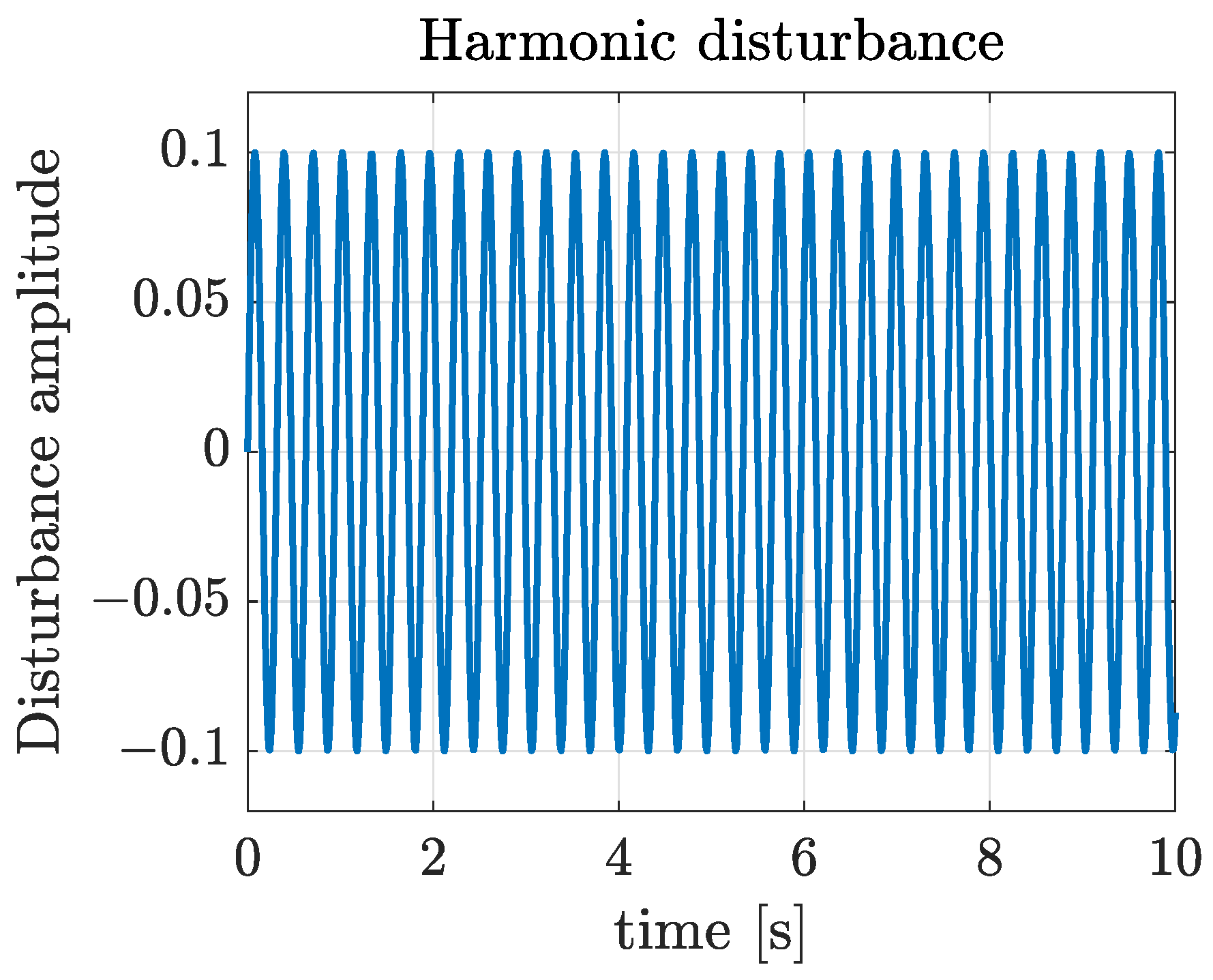
This section presents the numerical simulations conducted to demonstrate the superior performance of the proposed blended aerodynamic model over the traditional model in dealing with high AoA situations. Additionally, the effectiveness of the proposed HDO-STSMC-based control system in mitigating the effects of harmonic disturbances and model uncertainty is illustrated. The system matrices of the harmonic disturbances are designed as in Figure 5 [32].
A = 0 ω 0 ω 0 0 , C = 1 0
where ω 0 is the frequency of the harmonic disturbances and was set as 20 to emphasize its fast-changing characteristic.
Two performance indices, the integral of the square of the error (ISE) and the integral of the absolute magnitude (IAE), were used to further evaluate the tracking performances of the longitudinal states with the proposed blended aerodynamic model and the control system. The ISE is a suitable performance index to assess the control scheme performances of the longitudinal channels during the transition phase simulation and is defined as follows.
ISE = 0 T s e 2 t d t
where T s is the settling time.
The integral of the absolute magnitude (IAE) stems from the ISE and is widely used for computer simulation studies, expressed as follows.
IAE = 0 T e t d t
The minimization of the ISE or IAE criterion is often of practical significance and used to reflect the minimization of the fuel consumption of a UAV [42]. Moreover, the ISE and IAE emphasize different types of errors: the ISE places more weight on large error values instead of minor ones, which makes the ISE an effective way to measure the response time, while the IAE puts equal weight on all the errors regardless of their size, which makes it a straightforward way to evaluate the ability of the STSMC and the original SMC to retain the sliding manifold once the sliding surface is reached [43].
Table 5 provides the controller gains for the simulation.
The critical initial conditions of the four-channel simulations in the longitudinal dynamics are also provided in Table 6.

5.1. Comparative Results of the Blended and Traditional Aerodynamic Model

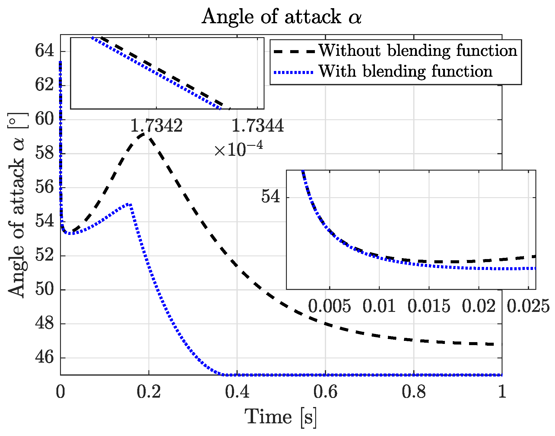
To figure out the necessity of introducing the nonlinear blending function to handle the high AoA situation during the transition phase, Figure 6 illustrated the fast change in the high AoA situation that the UAV faced when it entered the transition phase, from which one can see the necessity of blending the high AoA aerodynamic model with the low AoA one to deal with the flight situation beyond the stall angle ( α s = 12 ° for NACA9412). Moreover, Figure 6 revealed the UAV could handle the high AoA situation better with the blended aerodynamic model compared with the traditional one: the high AoA decreased quicker and was reduced to a smaller value with the nonlinear blending function.
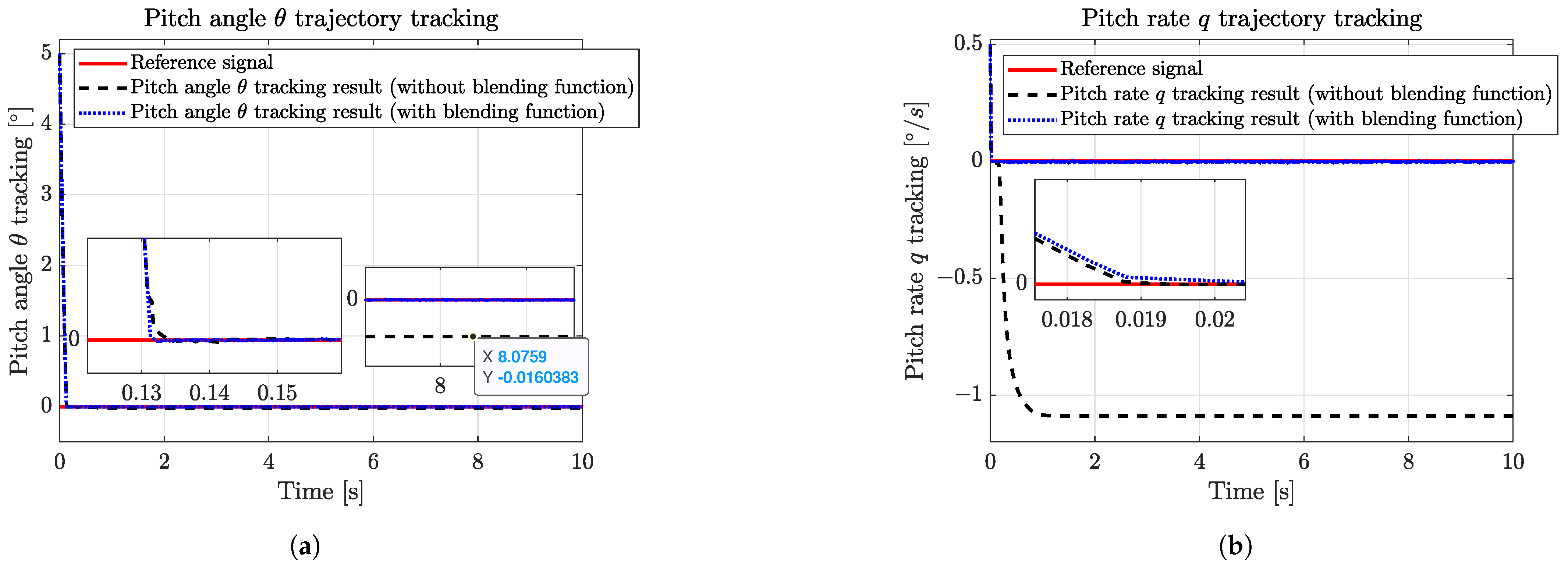
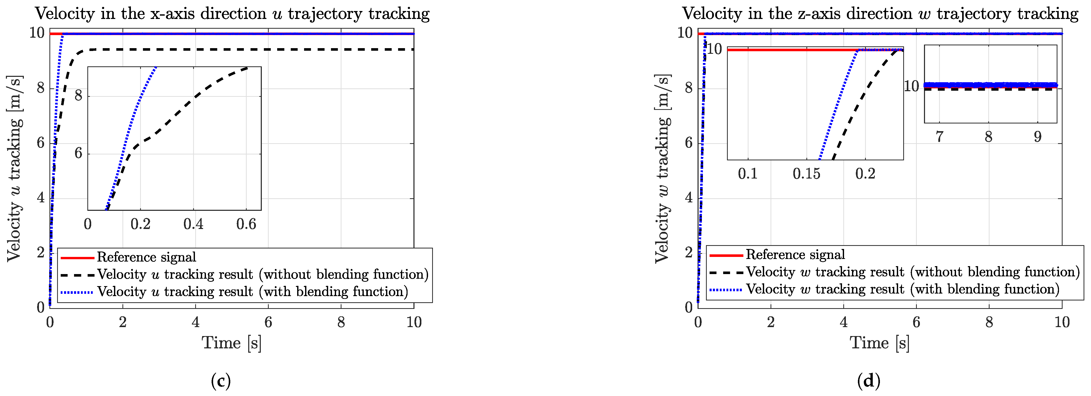
The comparative simulation of the longitudinal dynamics was carried out with the proposed HDO-STSMC control structure, and the comparative results of the state trajectory tracking (pitch angle θ , pitch rate q, velocity in the o x direction u, and velocity in the o z direction w) are illustrated in Figure 7. From this, one can quickly draw the first conclusion that with the same control scheme settings, the blended aerodynamic model can track the reference signals quicker and more accurately than the one without blending the high AoA aerodynamic model: the blended model resulted in the accurate tracking of the reference signals with no tracking errors and led to a reduction of 2.2%, 50%, 73.6%, and 11.2% in the time required for tracking the pitch angle, pitch rate, and velocities u and w, respectively; in contrast, the traditional model exhibited significant tracking errors ranging from 0.016° in the pitch angle channel to 1.25°/s in the pitch rate channel, 0.6 m/s for velocity u, and 0.01 m/s for velocity w.
Moreover, the tracking errors of the blended aerodynamic model all converged asymptotically, which was verified by the Lyapunov theory and the numerical results. Even if the traditional aerodynamic model can track the reference pitch angle θ (Figure 7a) and the reference velocity w (Figure 7d) almost as quickly with minor tracking errors, the time taken to reach the reference signals of the traditional aerodynamic model is longer than the blended one. The inadequacy of the traditional aerodynamic model is further highlighted by its inability to accurately track the reference signals of the velocity u (Figure 7c) and pitch rate q (Figure 7b). In contrast, the blended aerodynamic model successfully achieved fast and precise tracking of the reference signals for all the channels.
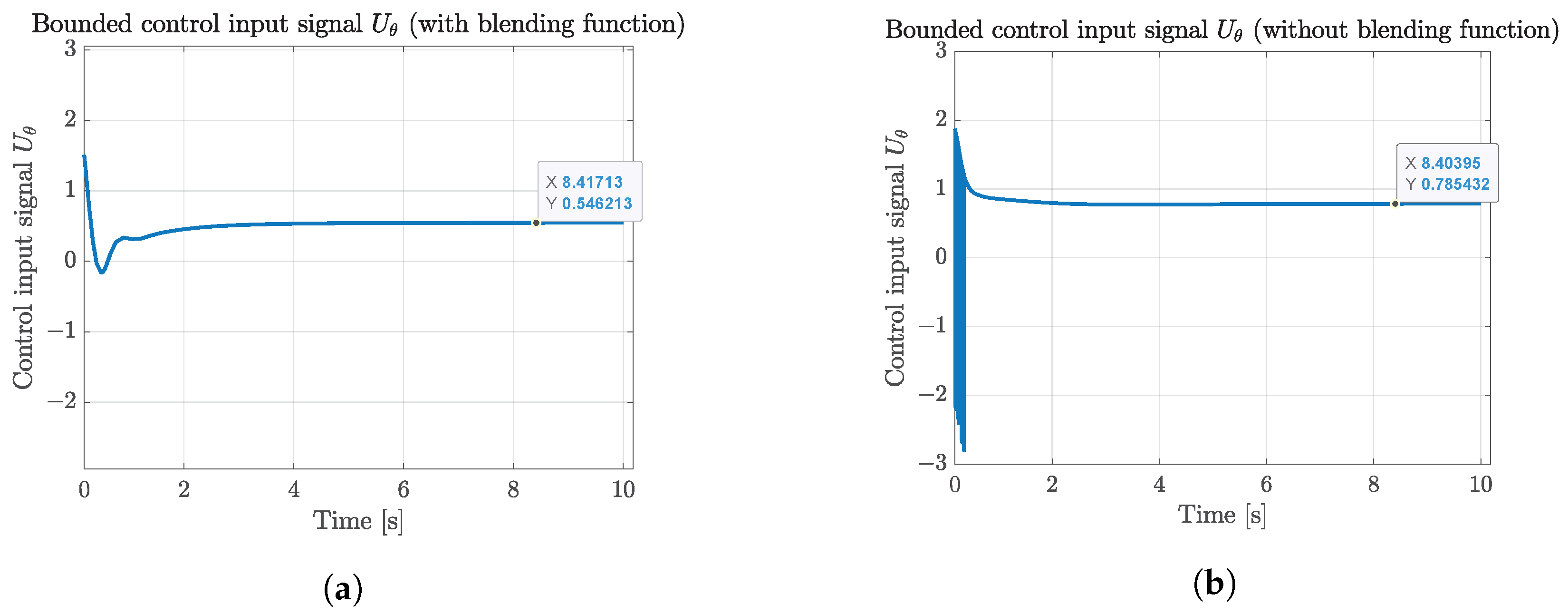
Furthermore, the comparative results of the control input signals are illustrated as follows, verifying the feasibility of the proposed HDO-STSMC control system and the asymptotic convergence of the state tracking errors presented in Figure 7. Furthermore, the bounded control input signals illustrated in Figure 8, Figure 9, Figure 10 and Figure 11 revealed the second important fact about the blended and traditional aerodynamic model: the blended aerodynamic model required a moderate control effort to achieve better tracking results compared with the traditional one. Like the one presented in reference [16], where the 2D-to-3D correction method was applied to solve the high AoA situation, the blended aerodynamic model is also feasible and requires less control effort in this study. More specifically, Figure 8a presents a smoother pitch angle θ control input signal of the blended aerodynamic model compared with the traditional one (
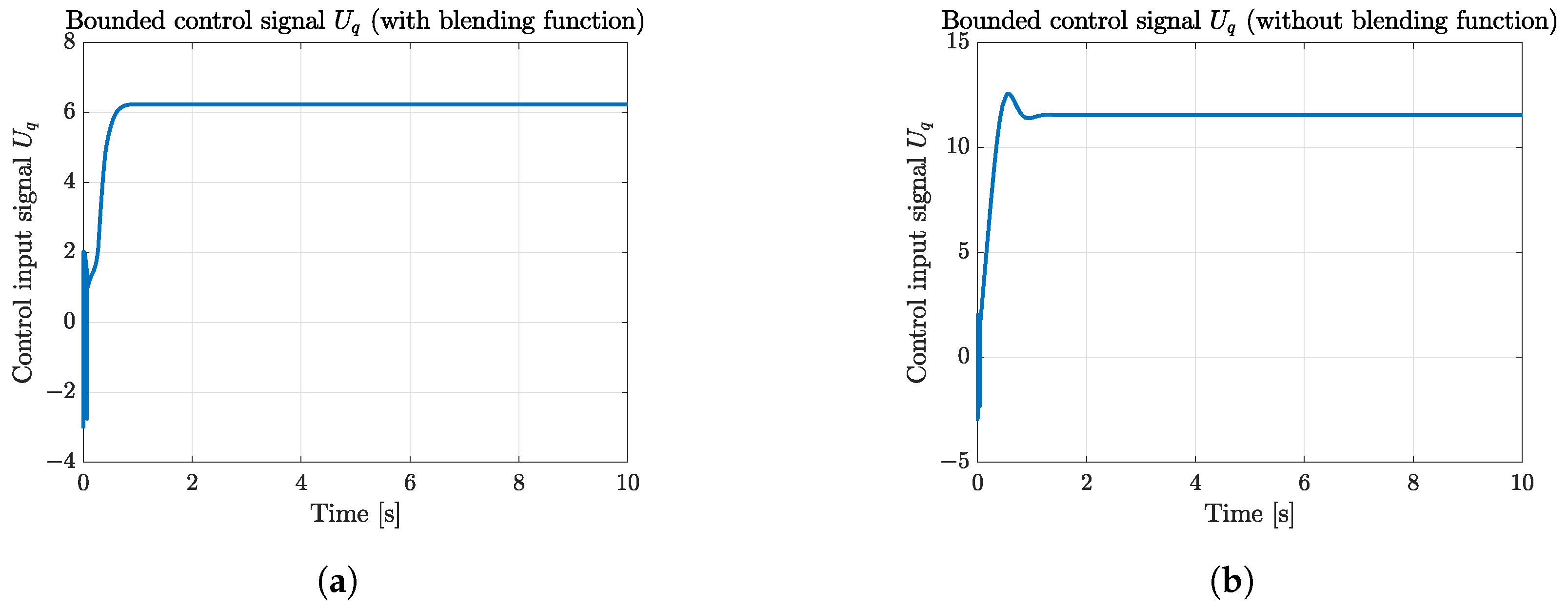
Figure 8b). Likewise, there was an overshooting in the pitch rate q control input signal illustrated in Figure 9b, while the control signal of the blended aerodynamic model is also smoother without overshooting (
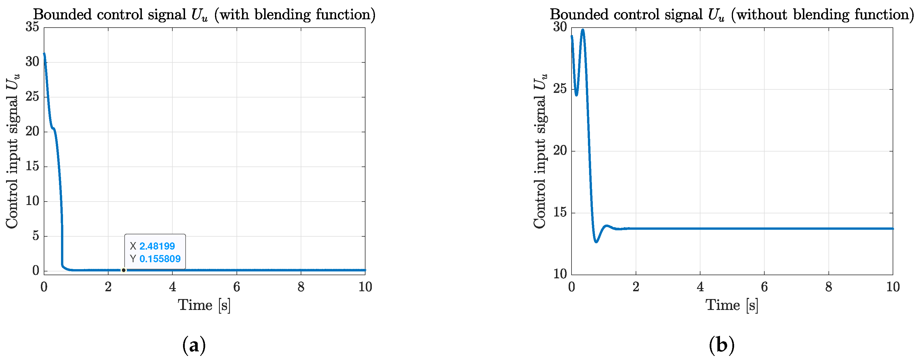
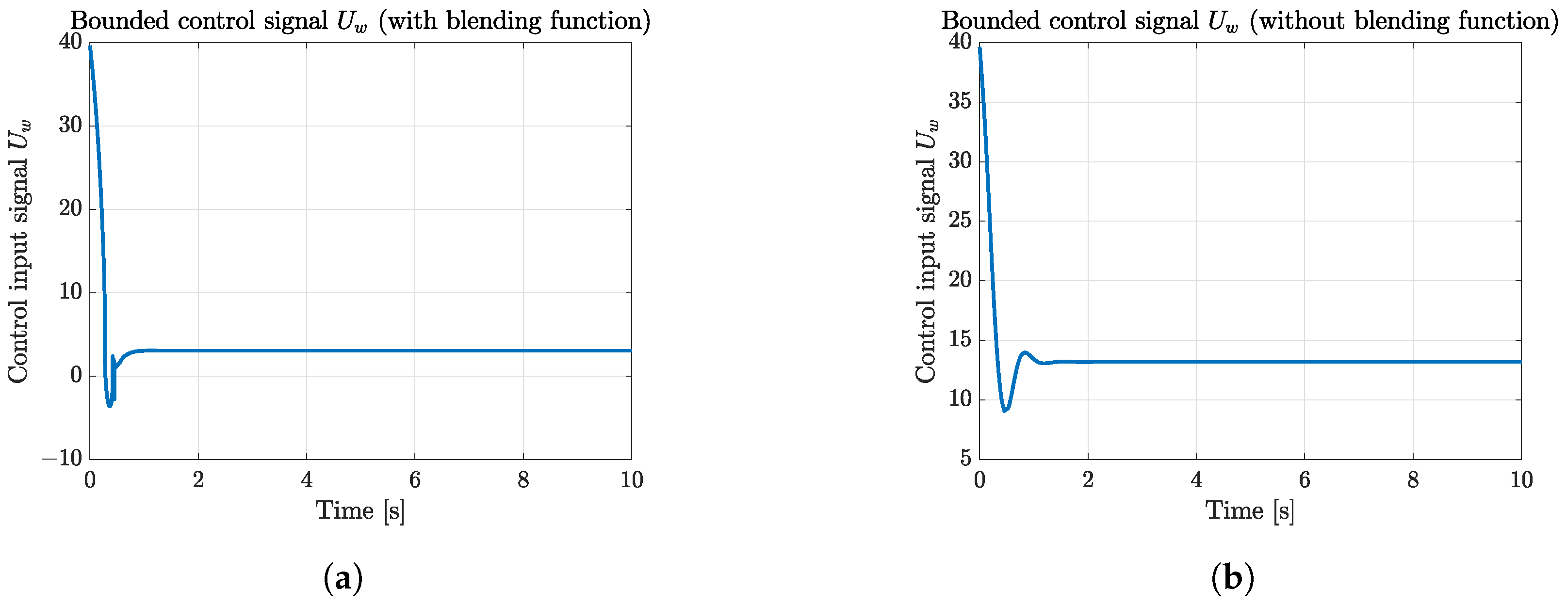
Figure 9a). The bounded control signals in the velocity channels of the blended aerodynamic model (Figure 10a and Figure 11a) still outperformed the ones of the traditional model (Figure 10b and Figure 11b) from the perspective of the response speed and control effort efficiency.
The ISE and IAE values of the blended and traditional aerodynamic model are presented in Table 7, from which one can tell the superiority of applying the blended aerodynamic model for the transition phase with much more minor tracking errors and a moderate control effort (a smaller value of the IAE indicates the better retention capability of the designed sliding manifolds and less required control effort).
Based on the comparative results of the blended and traditional aerodynamic models and the numerical analysis of the two performance indices, one can see the practical meaning of blending the high AoA model with the traditional one by using the proposed nonlinear blending function to handle the high AoA situation that the UAV encountered when it entered the transition phase. Moreover, the blended aerodynamic model can track the trajectory signals more quickly and accurately with the moderate control effort compared with the traditional one.

5.2. Comparative Results of the Proposed HDO-STSMC and the Original ESO-SMC

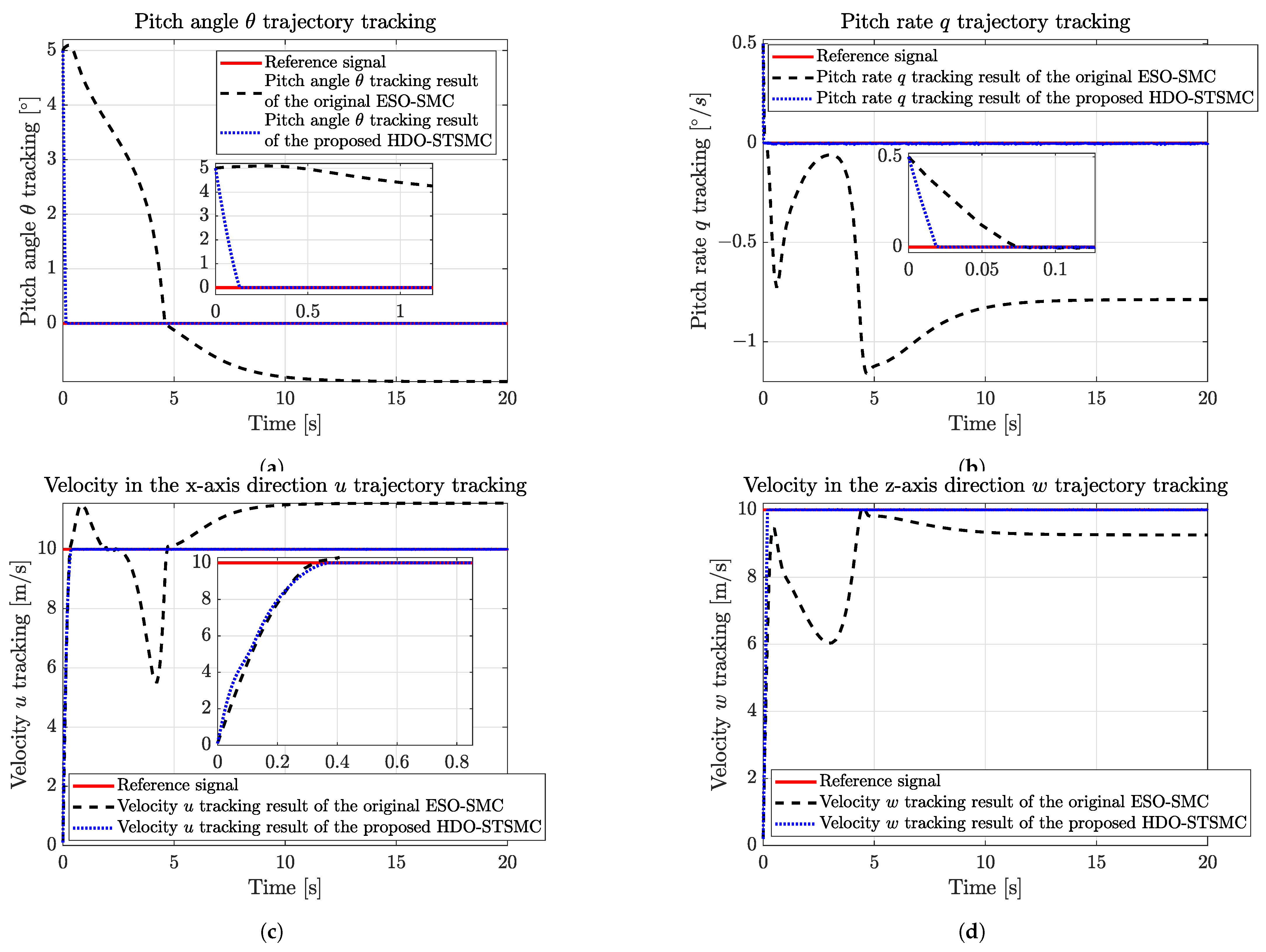
After verifying the superiority of the blended aerodynamic model, in this section, the comparative results of the proposed HDO-STSMC and the original ESO-SMC will be illustrated from the perspective of the state trajectory tracking performances and control signal inputs with the same blended aerodynamic model settings. The performance indices will also be used to evaluate these two control schemes.
The comparative results of the state trajectory tracking (the pitch angle θ , pitch rate q, velocity in the o x direction u, and velocity in the o z direction w) of the proposed HDO-STSMC and the original ESO-SMC are illustrated in Figure 12.
Based on Figure 12, it can be observed that the original ESO-SMC failed to accurately track all four reference state signals in the presence of external harmonic disturbances (as shown in Figure 5). Considerable tracking errors were observed, with 1.067° in the pitch angle channel, 0.788°/s in the pitch rate channel, 1.554 m/s for velocity u, and 0.746 m/s for velocity w, which served as evidence that the original ESO was unable to handle the fast-changing external disturbances effectively. Additionally, it took more time to converge, which increased the simulation time to 20 s as opposed to the 10 s in the previous section. On the contrary, the proposed HDO-STSMC can handle the harmonic disturbance better with zero tracking errors and a reduction of 97.2%, 73.6%, 11.3%, and 95.7% in the time required for tracking the pitch angle, pitch rate, and velocities u and w, respectively; the quick and accurate states tracking ability of the proposed HDO-STSMC-based control structure was also verified by the Lyapunov theory. Moreover, the STA also attenuated the chattering problems in the original SMC, leading to smoother tracking trajectories for the proposed HDO-STSMC.
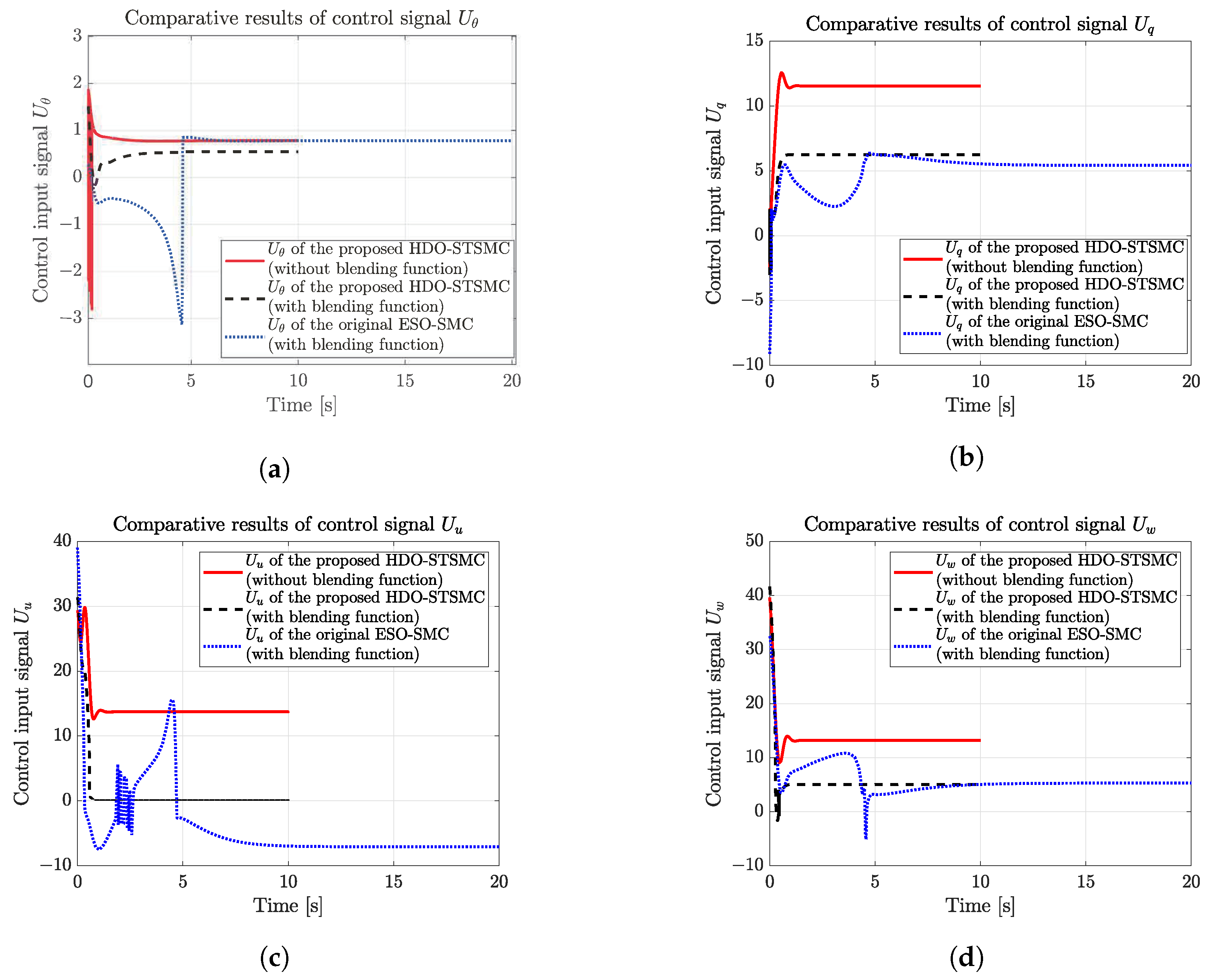
The comparative results of the control input signals are also illustrated in Figure 13, including the bounded control input signals of the proposed HDO-STSMC with the traditional aerodynamic model, the proposed HDO-STSMC with the blending function, and the original ESO-SMC with the blending function.
With the proposed blended aerodynamic model, comparing the bounded control input signals of the original ESO-SMC with the one obtained from the proposed HDO-STSMC, one can draw the first main conclusion about the superiority of the proposed HDO-STSMC: the control signals are smoother with quick convergence, which not only verified the feasibility of applying an HDO to deal with the fast-changing external disturbances but also verified the necessity of applying the STA to attenuate the chattering problems of the original SMC. More specifically, in the case of the pitch angle θ , the control input signal of the proposed HDO-STSMC displayed smoother characteristics when contrasted with that of the original ESO-SMC, which exhibited sharp amplitude changes around the 4.5 s mark. Similarly, the control input signal of the pitch rate q generated by the original ESO-SMC required twice as much time to converge as the proposed HDO-STSMC, and it featured more conspicuous changing signals. This outcome confirmed the feasibility and superiority of the proposed HDO-STSMC in handling external harmonic disturbances and model uncertainty. Oscillations were also evident in the velocity u channel of the original ESO-SMC, in contrast to the clearer and chattering-free signal produced by the proposed HDO-STSMC, which underscored the efficacy of the STA in attenuating chattering. Similar issues (slow convergence and sharp amplitude changes) also existed in the control input signal of the velocity w generated by the original ESO-SMC, compared with the one obtained from the proposed HDO-STSMC.
Moreover, the comparison between the bounded control input signal of the traditional aerodynamic model and that of the blended aerodynamic model yielded a second key conclusion, which revealed a moderate control effort with the blended aerodynamic model, and verified the outperformance of applying the blended aerodynamic model for the transition phase to deal with the high AoA situation. In contrast, the traditional low AoA aerodynamic model cannot properly address these conditions.
The ISE and IAE values of the proposed HDO-STSMC and the original ESO-SMC, including the pitch angle θ , pitch rate q, and velocities u and w, are presented in Table 8.
The high ISE values observed for the original ESO-SMC in Table 8 indicated its failure in tracking the trajectory due to its inability to handle fast-changing harmonic disturbances. On the other hand, the small IAE values obtained for the proposed HDO-STSMC demonstrated the remarkable ability of the STSMC to retain the designed sliding manifold once the variables reached the sliding surfaces. It is worth noting that the IAE values of the proposed HDO-STSMC with the blended aerodynamic model presented in Table 7 were calculated over a duration of 10 s, while the IAE values of the proposed HDO-STSMC with the blended aerodynamic model presented in Table 8 were calculated over a duration of 20 s, as the original ESO-SMC took double the time to converge. This explained the slight differences in the numerical values and further confirmed the superiority of applying the STA to the original SMC, leading to a better attachment to the sliding surfaces and the alleviation of the chattering problems.

6. Conclusions

The introduction of the blended aerodynamic model to handle high AoA situations and the implementation of the HDO-STSMC robust control scheme to attenuate fast-changing external disturbances along with the chattering problems resulted in more accurate and quicker longitudinal trajectory tracking results with moderate control effort, as demonstrated in this paper.
The first main conclusion of this paper is that the trajectory tracking results of the blended aerodynamic model outperformed the traditional one with zero tracking errors and a significant reduction of 2.2%, 50%, 73.6%, and 11.2% in the time required for tracking the pitch angle, pitch rate, and velocities u and w. Moreover, the blended aerodynamic model required less control effort, which verified the necessity and feasibility of introducing the nonlinear blending function to aggregate the flat-plate mode and linear mode of the aerodynamic coefficients, so that a smooth and continuous relationship between the aerodynamic coefficients and AoA can be obtained to handle the high AoA situation that the UAV faced during the transition phase.
The second significant finding is that the proposed HDO-STSMC outperformed the original ESO-SMC in tracking the state reference signals more accurately and quickly, which can be verified by the zero tracking errors with a reduction of 97.2%, 73.6%, 11.3%, and 95.7% in the time required for tracking the pitch angle, pitch rate, and velocities u and w, respectively. The HDO can estimate fast-changing external disturbances more accurately than the ESO, while the STA attenuated the chattering action and ensured a robust performance. The robust stability of the STSMC and HDO was proven via the Lyapunov theory. The converged tracking errors and bounded control input signals can also demonstrate the asymptotic stability of the closed-loop longitudinal autopilot system.
Performance indices (ISE and IAE) were used to evaluate the proposed HDO-STSMC longitudinal autopilot from the perspective of the response time and retaining capability on the sliding manifold, highlighting the robust stability and quick convergence of the system states to the reference signals. Furthermore, the comparative numerical results between the proposed HDO-STSMC and the original ESO-SMC confirmed the superior performance of the proposed control scheme in handling harmonic disturbances with an HDO and suppressing chattering with the STA.

Author Contributions

Conceptualization, J.L. and H.B.; methodology, J.L.; software, J.L.; validation, J.L.; formal analysis, J.L.; investigation, J.L.; resources, H.B.; data curation, J.L.; writing—original draft preparation, J.L.; writing—review and editing, H.B.; visualization, J.L.; supervision, H.B.; project administration, H.B.; funding acquisition, H.B. All authors have read and agreed to the published version of the manuscript.

Funding

This work was supported by the National Research Foundation of Korea (NRF) grant funded by the Ministry of Science and ICT (NRF-2017R1A5A1015311).

Institutional Review Board Statement

Not applicable.

Informed Consent Statement

Not applicable.

Data Availability Statement

Not applicable.

Conflicts of Interest

The authors declare no conflict of interest.

References

  1. Flores, G.R.; Escareño, J.; Lozano, R.; Salazar, S. Quad-tilting rotor convertible mav: Modeling and real-time hover flight control. J. Intell. Robot. Syst. 2012, 65, 457–471. [Google Scholar] [CrossRef] [Green Version]
  2. Yuksek, B.; Vuruskan, A.; Ozdemir, U.; Yukselen, M.; Inalhan, G. Transition flight modeling of a fixed-wing VTOL UAV. J. Intell. Robot. Syst. 2016, 84, 83–105. [Google Scholar] [CrossRef]
  3. Wang, X.; Cai, L. Mathematical modeling and control of a tilt-rotor aircraft. Aerosp. Sci. Technol. 2015, 47, 473–492. [Google Scholar] [CrossRef] [Green Version]
  4. Rohr, D.; Studiger, M.; Stastny, T.; Lawrance, N.R.; Siegwart, R. Nonlinear model predictive velocity control of a VTOL tiltwing UAV. IEEE Robot. Autom. Lett. 2021, 6, 5776–5783. [Google Scholar] [CrossRef]
  5. Li, B.; Sun, J.; Zhou, W.; Wen, C.Y.; Low, K.H.; Chen, C.K. Transition optimization for a VTOL tail-sitter UAV. IEEE/ASME Trans. Mechatronics 2020, 25, 2534–2545. [Google Scholar] [CrossRef]
  6. Lu, G.; Cai, Y.; Chen, N.; Kong, F.; Ren, Y.; Zhang, F. Trajectory Generation and Tracking Control for Aggressive Tail-Sitter Flights. arXiv 2022, arXiv:2212.11552. [Google Scholar]
  7. Flores, A.; Flores, G. Implementation of a Neural Network for Nonlinearities Estimation in a Tail-Sitter Aircraft. J. Intell. Robot. Syst. 2021, 103, 22. [Google Scholar] [CrossRef]
  8. Liao, J.; Song, X. Mathematical modelling and model predictive controller design of a quad tiltrotor UAV. Proc. Inst. Mech. Eng. Part C J. Mech. Eng. Sci. 2020, 0954406220971330. [Google Scholar] [CrossRef]
  9. Hegde, N.T.; George, V.; Nayak, C.G.; Vaz, A.C. Application of robust H-infinity controller in transition flight modeling of autonomous VTOL convertible Quad Tiltrotor UAV. Int. J. Intell. Unmanned Syst. 2021, 9, 204–235. [Google Scholar] [CrossRef]
  10. Kong, Z.; Lu, Q. Mathematical modeling and modal switching control of a novel tiltrotor UAV. J. Robot. 2018, 2018, 8641731. [Google Scholar] [CrossRef]
  11. Rushdi, M.; Hussein, A.; Dief, T.N.; Yoshida, S.; Schmehl, R. Simulation of the transition phase for an optimally-controlled tethered vtol rigid aircraft for airbornewind energy generation. In Proceedings of the AIAA SciTech 2020 Forum, Orlando, FL, USA, 6–10 January 2020; p. 1243. [Google Scholar]
  12. Yuksek, B.; Inalhan, G. Transition Flight Control System Design for Fixed-Wing VTOL UAV: A Reinforcement Learning Approach. In Proceedings of the AIAA SCITECH 2022 Forum, San Diego, CA, USA, 3–7 January 2022; p. 0879. [Google Scholar]
  13. Prieto, V.M.; Esteban, S. Wind Tunnel Aerodynamic Study of a VTOL-UAV for Wide Range of Angles of Attack and Sideslip Angles. Aerotec. Missili Spaz. 2020, 100, 39–55. [Google Scholar] [CrossRef]
  14. Pham, D.N.; Voet, L.; Kunycky, A.; Tan, C.S. Framework of a Power Management System for a Hybrid Electric VTOL Aircraft using Optimal Control. In Proceedings of the AIAA AVIATION 2022 Forum, Chicago, IL, USA, 27 June–1 July 2022; p. 3568. [Google Scholar]
  15. Selig, M. Modeling full-envelope aerodynamics of small UAVs in realtime. In Proceedings of the AIAA Atmospheric Flight Mechanics Conference, Toronto, ON, Canada, 2–5 August 2010; p. 7635. [Google Scholar]
  16. Di Francesco, G.; Mattei, M. Modeling and incremental nonlinear dynamic inversion control of a novel unmanned tiltrotor. J. Aircr. 2016, 53, 73–86. [Google Scholar] [CrossRef]
  17. Shi, X.; Kim, K.; Rahili, S.; Chung, S.J. Nonlinear control of autonomous flying cars with wings and distributed electric propulsion. In Proceedings of the 2018 IEEE Conference on Decision and Control (CDC), Miami, FL, USA, 17–19 December 2018; pp. 5326–5333. [Google Scholar]
  18. Beard, R.; McLain, T. Small Unmanned Aircraft: Theory and Practice; Princeton University Press: Princeton, NJ, USA, 2022. [Google Scholar]
  19. Kikumoto, C.; Urakubo, T.; Sabe, K.; Hazama, Y. Back-Transition Control With Large Deceleration for a Dual Propulsion VTOL UAV Based on Its Maneuverability. IEEE Robot. Autom. Lett. 2022, 7, 11697–11704. [Google Scholar] [CrossRef]
  20. Willis, J.B.; Beard, R.W. Pitch and Thrust Allocation for Full-Flight-Regime Control of Winged eVTOL UAVs. IEEE Control Syst. Lett. 2021, 6, 1058–1063. [Google Scholar] [CrossRef]
  21. Bannwarth, J.X.J. Aerodynamic Modelling and Wind Disturbance Rejection of Multirotor Unmanned Aerial Vehicles. Ph.D. Thesis, The University of Auckland, Auckland, New Zealand, 2022. [Google Scholar]
  22. Wang, Y.; Feng, Y.; Zhang, X.; Liang, J. A new reaching law for antidisturbance sliding-mode control of PMSM speed regulation system. IEEE Trans. Power Electron. 2019, 35, 4117–4126. [Google Scholar] [CrossRef]
  23. Levant, A. Sliding order and sliding accuracy in sliding mode control. Int. J. Control 1993, 58, 1247–1263. [Google Scholar] [CrossRef]
  24. Dai, B.; He, Y.; Zhang, G.; Gu, F.; Yang, L.; Xu, W. Wind disturbance rejection for unmanned aerial vehicle based on acceleration feedback method. In Proceedings of the 2018 IEEE Conference on Decision and Control (CDC), Miami, FL, USA, 17–19 December 2018; pp. 4680–4686. [Google Scholar]
  25. Khankalantary, S.; Sheikholeslam, F. Robust extended state observer-based three dimensional integrated guidance and control design for interceptors with impact angle and input saturation constraints. ISA Trans. 2020, 104, 299–309. [Google Scholar] [CrossRef] [PubMed]
  26. González, J.A.C.; Salas-Peña, O.; De León-Morales, J. Observer-based super twisting design: A comparative study on quadrotor altitude control. ISA Trans. 2021, 109, 307–314. [Google Scholar] [CrossRef]
  27. Chen, A.J.; Sun, M.J.; Wang, Z.H.; Feng, N.Z.; Shen, Y. Attitude trajectory tracking of quadrotor UAV using super-twisting observer-based adaptive controller. Proc. Inst. Mech. Eng. Part G J. Aerosp. Eng. 2021, 235, 1146–1157. [Google Scholar] [CrossRef]
  28. Shi, D.F.; Hou, Y.L.; Gu, X.H.; Hou, R.M. A Novel Active Disturbance Rejection Control with a Super-Twisting Observer for the Rocket Launcher Servo System. Shock Vib. 2021, 2021, 6617599. [Google Scholar] [CrossRef]
  29. Shi, D.; Wu, Z.; Chou, W. Super-twisting extended state observer and sliding mode controller for quadrotor uav attitude system in presence of wind gust and actuator faults. Electronics 2018, 7, 128. [Google Scholar] [CrossRef] [Green Version]
  30. Chen, M.; Xiong, S.; Wu, Q. Tracking flight control of quadrotor based on disturbance observer. IEEE Trans. Syst. Man Cybern. Syst. 2019, 51, 1414–1423. [Google Scholar] [CrossRef]
  31. Shi, D.; Wu, Z.; Chou, W. Harmonic extended state observer based anti-swing attitude control for quadrotor with slung load. Electronics 2018, 7, 83. [Google Scholar] [CrossRef] [Green Version]
  32. Chen, W.H. Harmonic disturbance observer for nonlinear systems. J. Dyn. Syst. Meas. Control 2003, 125, 114–117. [Google Scholar] [CrossRef]
  33. Chen, W.H. Nonlinear disturbance observer based control for nonlinear systems with harmonic disturbances. IFAC Proc. Vol. 2001, 34, 329–334. [Google Scholar] [CrossRef]
  34. Chen, W.H. Disturbance observer based control for nonlinear systems. IEEE/ASME Trans. Mechatron. 2004, 9, 706–710. [Google Scholar] [CrossRef] [Green Version]
  35. Ha, L.N.N.T.; Hong, S.K. Robust dynamic sliding mode control-based PID–super twisting algorithm and disturbance observer for second-order nonlinear systems: Application to UAVs. Electronics 2019, 8, 760. [Google Scholar] [CrossRef] [Green Version]
  36. Zhou, Z.; Yao, S.; Ma, C.; Zhang, G.; Geng, Q. Design of High-Dynamic PMSM Servo Drive Using Nonlinear Predictive Controller with Harmonic Disturbance Observer. Energies 2022, 15, 4107. [Google Scholar] [CrossRef]
  37. Pavan, N. Design of Tiltrotor VTOL and Development of Simulink Environment for Flight Simulations. Master’s Thesis, Indian Institute of Space Science and Technology, Kerala, India, 2020. [Google Scholar]
  38. Arifianto, O.; Farhood, M. Optimal control of a small fixed-wing UAV about concatenated trajectories. Control Eng. Pract. 2015, 40, 113–132. [Google Scholar] [CrossRef]
  39. Shtessel, Y.; Edwards, C.; Fridman, L.; Levant, A. Sliding Mode Control and Observation; Springer: Berlin, Germany, 2014; Volume 10. [Google Scholar]
  40. Moreno, J.A.; Osorio, M. Strict Lyapunov functions for the super-twisting algorithm. IEEE Trans. Autom. Control 2012, 57, 1035–1040. [Google Scholar] [CrossRef]
  41. Isidori, A. Nonlinear Control Systems: An Introduction; Springer: Berlin, Germany, 1985. [Google Scholar]
  42. Dorf, R.C.; Bishop, R.H. Modern Control Systems; Pearson Prentice Hall: Hoboken, NJ, USA, 2008. [Google Scholar]
  43. Griffiths, J.B. Multivariable Super-Twisting Control of Fixed-Wing UAVs. Master’s Thesis, Norwegian University of Science and Technology NTNU, Trondheim, Norway, 2021. [Google Scholar]
Figure 1. Quad tiltrotor UAV configuration and the generalized body-fixed frame o x y z with the origin o coincident with the center of gravity c g .
Drones 07 00255 g001
Figure 2. Aerodynamic coefficients C L α , C D α , and C M α of NACA9412 with angle of attack α range 180 ° , 180 ° .
Drones 07 00255 g002
Figure 3. Graphical interpretation of the basic sliding mode control with the reaching phase starting from x 0 to the sliding phase, and the chattering phenomena occur on the sliding manifold s = k e + e d t .
Drones 07 00255 g003
Figure 4. Block structure of the proposed HDO-STSMC longitudinal controller for quad tiltrotor UAV: HDO is used to estimate the external harmonic disturbances, and STSMC is used to compensate for the estimated disturbances and handle the model uncertainty.
Drones 07 00255 g004
Figure 5. Fast-changing harmonic disturbance.
Drones 07 00255 g005
Figure 6. The fast change in high AoA during the transition phase.
Drones 07 00255 g006
Figure 7. Longitudinal states ( θ , q, u, and w) trajectory tracking comparative results of the blended and traditional aerodynamic model. (a) Pitch angle θ trajectory tracking comparative results of the blended and traditional aerodynamic model. (b) Pitch rate q trajectory tracking comparative results of the blended and traditional aerodynamic model. (c) Velocity in the o x direction u trajectory tracking comparative results of the blended and traditional aerodynamic model. (d) Velocity in the o z direction w trajectory tracking comparative results of the blended and traditional aerodynamic model.
Drones 07 00255 g007aDrones 07 00255 g007b
Figure 8. Pitch angle θ bounded control input signal comparative results of the blended and traditional aerodynamic model. (a) Pitch angle θ bounded control input signal U θ of the blended aerodynamic model. (b) Pitch angle θ bounded control input signal U θ of the traditional aerodynamic model.
Drones 07 00255 g008
Figure 9. Pitch rate q bounded control input signal comparative results of the blended and traditional aerodynamic model. (a) Pitch rate q bounded control input signal U q of the blended aerodynamic model. (b) Pitch rate q bounded control input signal U q of the traditional aerodynamic model.
Drones 07 00255 g009
Figure 10. Velocity u bounded control input signal comparative results of the blended and traditional aerodynamic model. (a) Velocity u bounded control input signal U u of the blended aerodynamic model. (b) Velocity u bounded control input signal U u of the traditional aerodynamic model.
Drones 07 00255 g010
Figure 11. Velocity w bounded control input signal comparative results of the blended and traditional aerodynamic model. (a) Velocity w bounded control input signal U w of the blended aerodynamic model. (b) Velocity w bounded control input signal U w of the traditional aerodynamic model.
Drones 07 00255 g011
Figure 12. Longitudinal states ( θ , q, u, and w) trajectory tracking comparative results of the proposed HDO-STSMC and the original ESO-SMC. (a) Pitch angle θ trajectory tracking comparative results of the proposed HDO-STSMC and the original ESO-SMC. (b) Pitch rate q trajectory tracking comparative results of the proposed HDO-STSMC and the original ESO-SMC. (c) Velocity in the o x direction u trajectory tracking comparative results of the proposed HDO-STSMC and the original ESO-SMC. (d) Velocity in the o z direction w trajectory tracking comparative results of the proposed HDO-STSMC and the original ESO-SMC.
Drones 07 00255 g012
Figure 13. The comparative results of bounded control input signals of the proposed HDO-STSMC with the traditional aerodynamic model, the proposed HDO-STSMC with blending function, and the original ESO-SMC with blending function. (a) The comparative results of bounded control input signal U θ . (b) The comparative results of bounded control input signal U q . (c) The comparative results of bounded control input signal U u . (d) The comparative results of bounded control input signal U w .
Drones 07 00255 g013
Table 1. Aerodynamic parameter values for Equation (5).
SymbolsDescriptionsValues
C L 0 Lift coefficient at zero AoA0.81857
C L α Lift slope4.09127
C D 0 Drag coefficient at zero AoA0.0294
C D α 1 -0.3673
C D α 2 -2.2229
C M 0 Pitching moment coefficient at zero AoA0.00763
C M α Pitching moment slope−1.76966
Table 2. Parameter values for blending function.
SymbolsValues
a L 1 0.7
a L 2 0.8
a L 3 0.8
a D 1 1.0
a D 2 1.0
a D 3 1.0
a M 1 0.5
a M 2 0.5
a M 3 0.5
R50
α s 12 °
Table 3. Structure parameter values for rotors.
Components o x ( m ) o z ( m )
Rotor 10.250
Rotor 20.250
Rotor 3−0.500
Rotor 4−0.500
Table 4. UAV parameters.
ParametersDescriptionsValues
mMass6 kg
SFixed-wing projected area0.550 m2
c ¯ Mean aerodynamic chord0.282 m
bWing span2 m
I y Moment of inertia around o y axis0.7893 kg · m2
k T Thrust coefficient0.1142 kg · m
k D Torque coefficient0.007048 kg · m2
Table 5. Controller gains in HDO-STSMC system.
ParametersDescriptionsValues
k 1 i ( i = θ , q , u , w ) Super-twisting control gain (Equation (13)) d i a g [ 4 , 4 , 4 , 4 ]
k 2 i ( i = θ , q , u , w ) Super-twisting control gain (Equation (13)) d i a g [ 2 , 2 , 2 , 2 ]
k i ( i = θ , q , u , w ) Sliding manifolds control gains (Equation (25)) d i a g [ 2 , 2 , 2 , 2 ]
k 1 i ( i = θ , q , u , w ) Harmonic disturbance observer control gains d i a g [ 0.01 , 0.01 , 0.01 , 0.01 ]
Table 6. The critical initial conditions of the simulation.
VariablesDescriptionsValues
θ 0 Initial pitch angle
θ r e f Reference pitch angle
q 0 Initial pitch rate0.5°/s
q r e f Reference pitch rate0°/s
u 0 Initial velocity in the o x -axis direction0.1 m/s
u r e f Reference velocity in the o x -axis direction10 m/s
w 0 Initial velocity in the o z -axis direction0.2 m/s
w r e f Reference velocity in the o z -axis direction10 m/s
Table 7. Performance index results of the blended and traditional aerodynamic model.
UAV Dynamic ModelVariablesISEIAE
Blended aerodynamic model θ 0.9433 ° 0.2957 °
q0.0018°/s0.0342°/s
u6.4818 m/s1.1995 m/s
w6.5748 m/s1.0082 m/s
Traditional aerodynamic model θ 0.9457°0.4490°
q11.4042°/s10.5551°/s
u12.3537 m/s7.4418 m/s
w6.7607 m/s1.0818 m/s
Table 8. Performance index results of the proposed HDO-STSMC and the original ESO-SMC.
Control SchemesVariablesISEIAE
HDO-STSMC θ 0.9433°0.2969°
q0.0018°/s0.0642°/s
u6.4818 m/s1.2298 m/s
w6.5748 m/s1.0399 m/s
ESO-SMC θ 71.8126°29.2259°
q12.2382°/s14.5630°/s
u52.8511 m/s27.3866 m/s
w50.3326 m/s22.0267 m/s
Disclaimer/Publisher’s Note: The statements, opinions and data contained in all publications are solely those of the individual author(s) and contributor(s) and not of MDPI and/or the editor(s). MDPI and/or the editor(s) disclaim responsibility for any injury to people or property resulting from any ideas, methods, instructions or products referred to in the content.

