Article

Improved Crop Biomass Algorithm with Piecewise Function (iCBA-PF) for Maize Using Multi-Source UAV Data

1
College of Geodesy and Geomatics, Shandong University of Science and Technology, Qingdao 266590, China
2
Key Laboratory of Crop Physiology and Ecology, Institute of Crop Sciences, Chinese Academy of Agricultural Sciences, Ministry of Agriculture, Beijing 100081, China
3
National Nanfan Research Institute (Sanya), Chinese Academy of Agricultural Sciences, Sanya 572024, China
4
College of Computer Science and Engineering, Shandong University of Science and Technology, Qingdao 266590, China
*
Authors to whom correspondence should be addressed.
These authors contributed equally to this work.
Drones 2023, 7(4), 254; https://doi.org/10.3390/drones7040254
Submission received: 18 February 2023 / Revised: 29 March 2023 / Accepted: 5 April 2023 / Published: 8 April 2023

Abstract

:
Maize is among the most important grain crops. Aboveground biomass (AGB) is a key agroecological indicator for crop yield prediction and growth status monitoring, etc. In this study, we propose two new methods, improved crop biomass algorithm (iCBA) and iCBA with piecewise function (iCBA-PF), to estimate maize AGB. Multispectral (MS) images, visible-band (RGB) images, and light detection and ranging (LiDAR) data were collected using unmanned aerial vehicles (UAVs). Vegetation indices (VIs) and the VI-weighted canopy volume model (CVMVI) were calculated and used as input variables for AGB estimation. The two proposed methods and three benchmark methods were compared. Results demonstrated that: (1) The performance of MS and RGB data in AGB estimation was similar. (2) AGB was estimated with higher accuracy using CVMVI than using VI, probably because the temporal trends of CVMVI and AGB were similar in the maize growing season. (3) The best estimation method was the iCBA-PF (R2 = 0.90 ± 0.02, RMSE = 190.01 ± 21.55 g/m2), indicating that AGB before and after maize heading should be estimated with different methods. Our method and findings are possibly applicable to other crops with a heading stage.

1. Introduction

Maize is one of the most important grain crops in the world, provide at least 30% of food calories to billions of people in many developing countries [1,2]. A key agroecological indicator of maize is aboveground biomass (AGB) [3], which can be used to monitor crop growth, carbon storage, and physiological conditions [4]. To accurately measure the AGB of maize is critical for monitoring its growth, predicting yield [5], and guiding precision agriculture practices [6].
Traditionally, AGB is measured through destructive sampling, which is the most accurate method but is also time-consuming, labor intensive, destructive [7,8]. Remote sensing, as a means of obtaining target information from a distance, provides a non-destructive alternative for AGB estimation at a variety of spatial scales. At the global or regional scale, satellite remote sensing is often used to estimate the AGB of grassland or forests [9,10]. However, the main concern in crop AGB is at the field scale, requiring finer-spatial-resolution observations [7,11,12], which calls for the use of unmanned aerial vehicle (UAV) remote sensing.
UAV estimation of crop AGB has its unique advantages. It can carry a variety of sensors to obtain different data such as visible (red–green–blue, RGB) images, multispectral (MS) images, and light detection and ranging (LiDAR). Multiple sensors can be mounted simultaneously, which makes the data collection highly efficient. The flight height, flight time, spatial extent, and spatiotemporal resolution can be controlled for data collection. High-spatial-resolution UAV data have been used to estimate the AGB of different crops, such as rice [13], winter wheat [14], maize [7], and soybean [15]. Different accuracies have been reported (R2: 0.75–0.94, RMSE: 122–374 g/m2) depending on the data type, indicators, and estimation methods.
Indicators that have proved useful for AGB estimation include vegetation spectral indices (VIs), textural indices (TIs), and structural indicators (SIs). While each type of indicator can be used for AGB estimation with moderate accuracy [3,4,7,16], more and more studies have shown that combining multiple sources of information like spectral information and structural information led to higher accuracy. Xu et al. [17] combined spectral, structural, and textural features to estimate rice AGB, and obtained more accurate results than when excluding any features. Liu et al. [18] combined VIs and TIs extracted from MS data in partial least squares regression (PLSR) and random forest regression (RFR) to estimate the AGB of winter oilseed. They found that the estimation result obtained by combining VIs and TIs was more accurate than using VIs or TIs alone, regardless of the method. Maimaitijiang et al. [15] combined VI with an SI, the canopy volume model (CVM), and proposed the VI-weighted CVM (CVMVI) for soybean AGB estimation. The accuracy was significantly improved compared to using VI or CVM alone.
Compared with the modeling of AGB in the whole growing season, AGB is better estimated at pre-heading and post-heading stages separately [13,19]. Zheng et al. [19] used VIs and TIs from MS images to estimate rice AGB. They found that the estimation results at the pre-heading stage were significantly better than at the post-heading stage, which suggested that AGB estimation at the post-heading stage needed further improvement. Li et al. [13] came to a similar conclusion with SIs from LiDAR data. They found that the linear mixed-effects (LME) model considering the growth stage greatly improved the estimation of AGB at the post-heading stage. Li et al. [20] proposed the crop biomass algorithm (CBA) method, which improved the AGB estimation results of wheat by integrating phenological characteristics (Zadoks scale) and growing degree day (GDD) in the model.
Previous research results show that the ways to improve the accuracy of crop remote-sensing AGB estimation results mainly include (1) the improvement of indicators, such as the CVMVI proposed by Maimaitijiang et al. [15], (2) the improvement of methods, such as the CBA method proposed by Li et al. [20], and (3) the division of pre-heading and post-heading stages. However, these three means have rarely been combined.
The aim of this study is to develop a method of crop AGB estimation combining the advantages of indicator improvement, method improvement, and division of growth periods. More specifically, our study aims to (1) compare the MS and RGB data sources in AGB estimation, (2) explore the improvement of AGB estimation by CVMVI compared with VI, and (3) investigate the differences between our proposed method and the state-of-the-art methods.

2. Materials and Methods

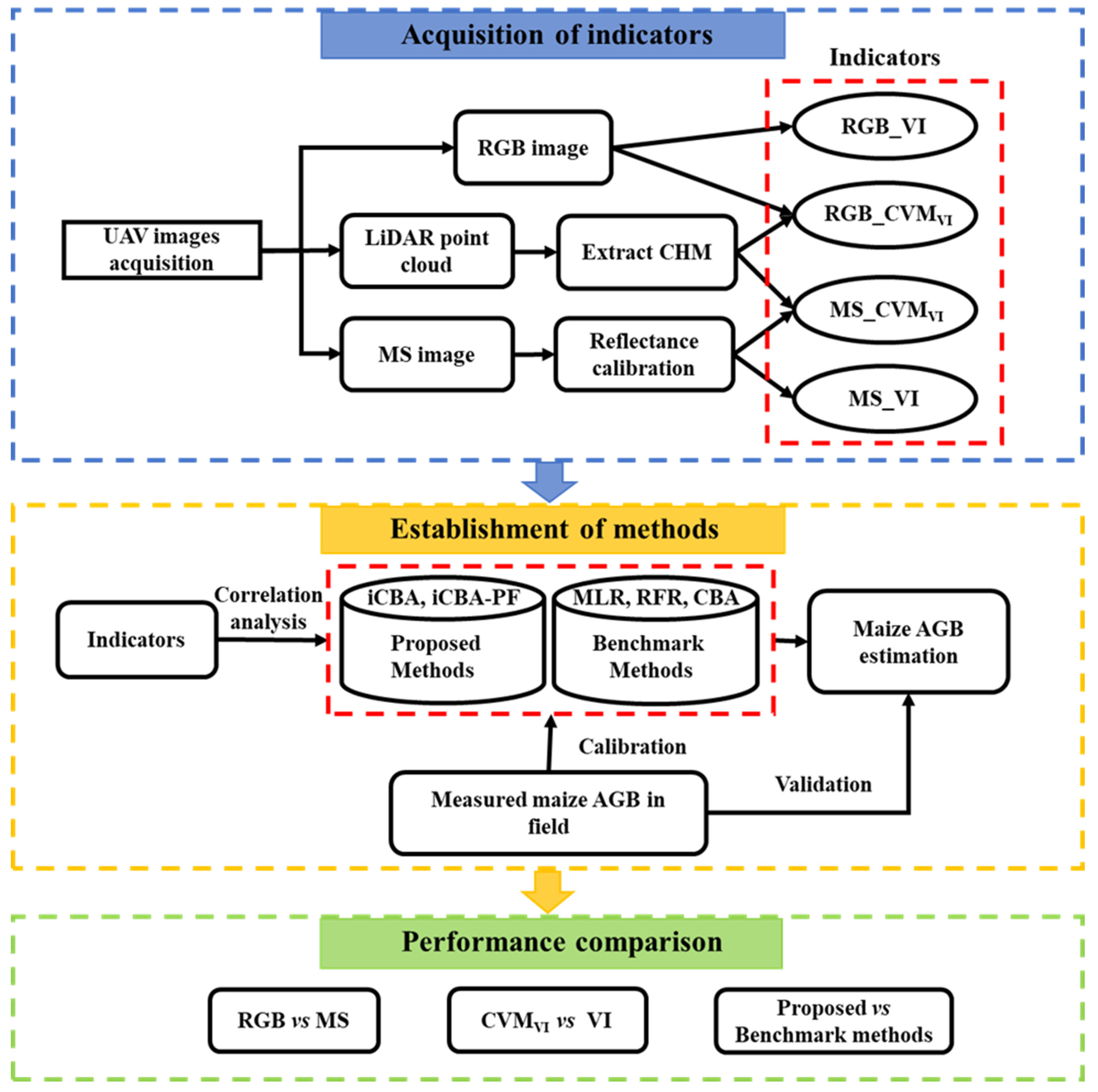
2.1. The Framework of the Article

The workflow of this study is shown in Figure 1. Firstly, four types of indicators were acquired from UAV data, including VIs from RGB images (RGB_VI), CVMVI using VIs from RGB images (RGB_CVMVI), CVMVI using VIs from MS images (MS_CVMVI), and VIs from MS images (MS_VI). These four types of indicators were then correlated with AGB to provide input variables for the five methods: multiple linear regression (MLR), RFR, CBA, improved CBA (iCBA), and piecewise iCBA (iCBA-PF). Finally, we compared the performance of data sources, indicators, and methods.

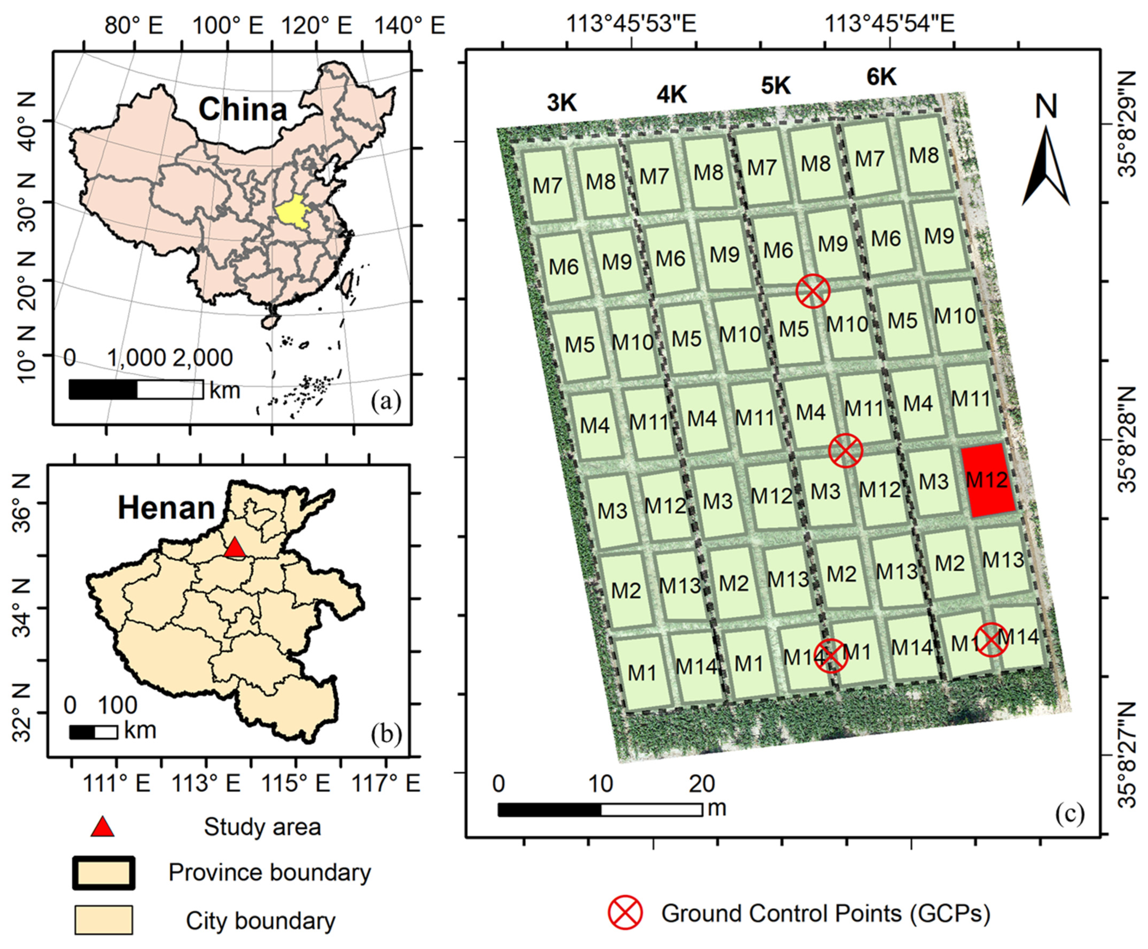
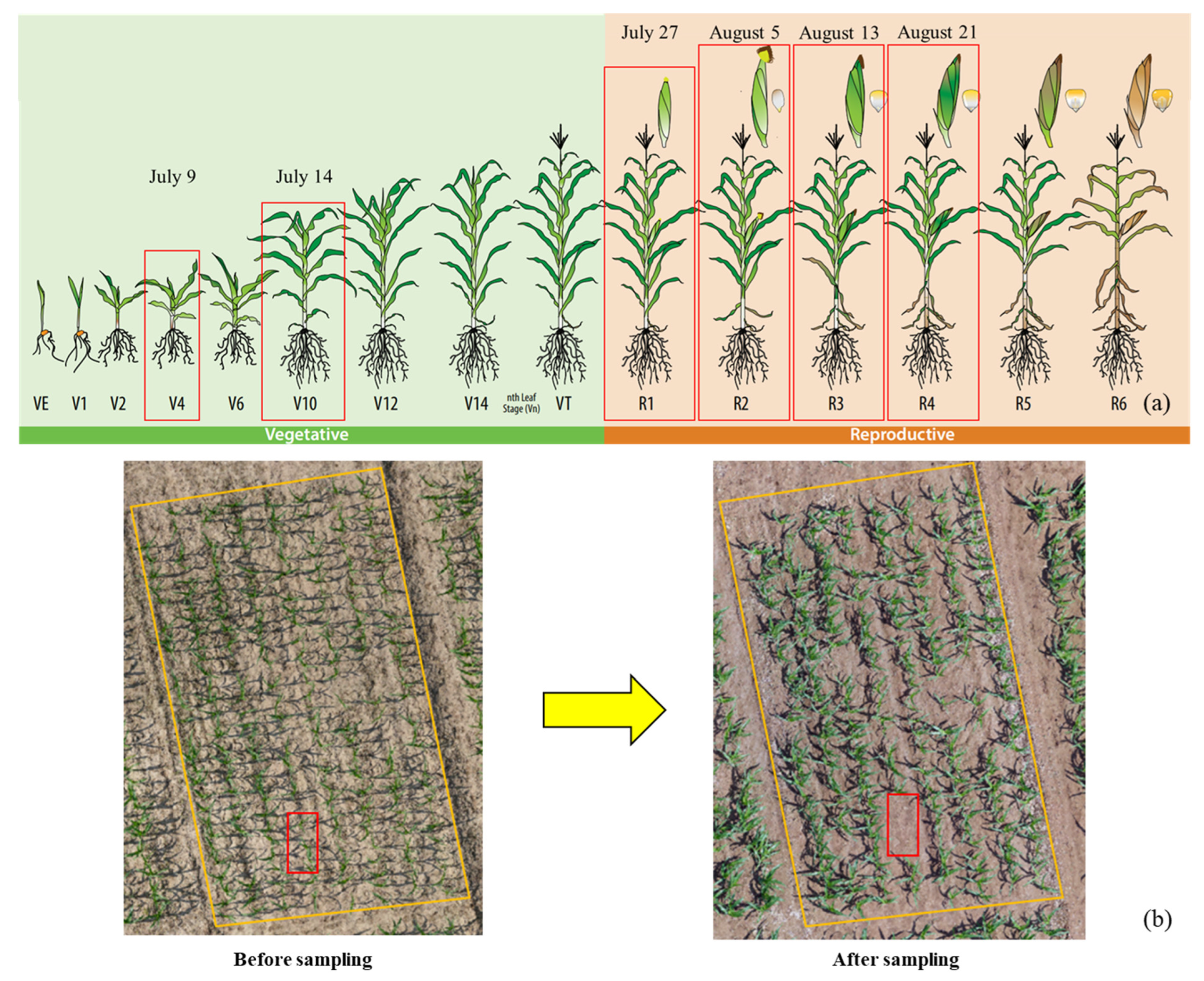
2.2. Study Sites and Experimental Design

Our study site is located at the Xinxiang experimental base of the Chinese Academy of Agricultural Sciences, Xinxiang City, Henan Province, China (35°8′ N, 113°45′ E) (Figure 2a,b). Xinxiang City is in the hinterland of the Central Plains and the north of Henan Province, in the Yellow River and Haihe River basins. There are 6.17 million permanent residents in Xinxiang City. The plain accounts for 78% of the total land area of the city. Xinxiang has a warm temperate continental monsoon climate with four distinct seasons: cold in winter, hot in summer, cool in autumn, and warm in spring. The average annual precipitation in Xinxiang City is 573.4 mm. The seasonal distribution of precipitation is extremely uneven, which is roughly consistent with the advance and retreat of winter and summer monsoons [21].
There were 56 plots in total, including four levels of density and 14 maize varieties (Figure 2c). The size of every plot was about 31.5 m2 (7.5 m × 4.2 m). Maize was planted on 16 June 2021 with 0.6 m row spacing. As shown in Figure 2c, the plant spacing was 0.370 m, 0.278 m, 0.222 m, and 0.185 m corresponding to the planting density of 3K, 4K, 5K, and 6K, respectively. The 3K–6K represents 3000–6000 plants per mu (1 mu = 666.67 m2), respectively, and M1-–M14 represents the 14 maize varieties, including Nongda 108, Zhengdan 958, Dika 517, Xinyu 108, SC 704, KWS 2030, Chidan 109, Jiuyu W03, MC 703, Heyu 187, MC 670, Kehe 699, MC 121, and Jingke 999. The amount of nitrogen application and irrigation in our experimental area were both consistent with different plots.

2.3. Data Acquisition and Pre-Processing

We conducted field measurements six times in 2021, as illustrated in Figure 3. In the vegetative growth stage of maize, we collected ground-truth biomass data on 9 July and 14 July 2021, respectively. In the reproductive growth stage, we collected ground-truth biomass data on 27 July, 5 August, 13 August, and 21 August, respectively. The maize plants in plot 6K-M12 (red rectangle in Figure 2c) were destroyed due to a storm in the middle of July 2021. Therefore, the samples of this plot after July 9 were abandoned. Thus, the total number of samples was 331, resulting from 56 samples in each growth stage multiplied by six sampling times and subtracting the five storm-destroyed samples in the 6K-M12 plot.
For the acquisition of each ground-truth sample, three representative maize plants (consecutive) were cut in each plot in each period, as shown in Figure 3b. Each plant was cut from two centimeters above the ground. The three plants were taken back to the laboratory for weighing. They were cut into small pieces and put into the oven to first de-enzyme under 105 °C for two hours and then dried at 80 °C until the weight did not change. The dry AGB was weighed using electronic balances with 0.1 g precision and scaled up to the unit of g/m2.
In this study, a hexacopter UAV, the DJI M600 pro (DJI Technology Co., Shenzhen, China), and a professional-grade quadrotor UAV, the DJI M300 RTK (DJI Technology Co., Shenzhen, China), were adopted to collect remote sensing data. A SONY A7R2 digital camera (Sony, Tokyo, Japan) and a Micasense rededge MX MS camera (Leptron Unmanned Aircraft Systems, Inc., Denver, CO, USA) were equipped on the DJI M600 Pro UAV to obtain RGB and MS images of the experimental area, respectively. The lateral and forward overlaps were 75% and 86%, respectively. The photo of a calibrated reflectance panel was taken before each flight to facilitate the radiometric calibration of the MS images. A LiDAR sensor DJI Zenmuse L1 (DJI Technology Co., Shenzhen, China) was equipped on the DJI M300 RTK to obtain LiDAR point cloud data. Four marks were placed and kept between the plots as ground control points (GCPs) (Figure 2) for geo-registration purposes.
The orthoimages of RGB and MS data were generated using the Agisoft PhotoScan software (version 1.4.5, Agisoft LLC, St. Petersburg, Russia). The LiDAR point cloud data was generated using the DJI Terra software (DJI Technology Co., Shenzhen, China). Georegistration of the orthoimages obtained at different times was conducted so that the positional displacements were removed and the images were geographically well aligned. This step was done in the ArcGIS software (version 10.6, ESRI, Inc., Redlands, CA, USA) according to the GCPs.
The data acquisition date, flight altitude (FA) and spatial resolution (SR) of the data are shown in Table 1. The SR of LiDAR is the average point spacing. The RGB and MS images were collected at 20 m FA on the first four dates (9 July to 31 July 2021). Due to unsolved practical issues, however, the RGB and MS data collected at 20 m FA on August 8 and August 18 could not be properly mosaicked. Therefore, we used images collected at higher FAs (30 m, 70 m, and 100 m) on these dates. The RGB image on 18 August 2021 were obtained with the DJI Zenmuse L1 sensor, which had lower SR than the SONY A7R2 images, despite the lower FA. The SR has been found to have little influence on the AGB estimation [15], and was ignored in this study.

2.4. UAV Data Processing

2.4.1. Sample Plant Mask Extraction

Each ground-truth AGB sample was represented by the weight of three plants, while the UAV data were spatially continuous. We have MS and RGB images both before and after sampling. Because the spatial resolution of the MS and RGB images are much higher than the plants (spatial resolution < 0.1 m, plant canopy width > 0.5 m), we can easily identify the three sampled plants by comparing the before and after images. To ensure the correspondence between the UAV data and the field measurements, we generated masks in the UAV data for the sampled plants. Firstly, the sampled plants were marked by digitization in the images collected immediately before the sampling. Then, soil pixels were removed by applying VI thresholds. Pixels in the RGB images with color index of vegetation (CIVE) larger than 18.10 were recognized as soil, while pixels in the MS images with normalized difference vegetation index (NDVI) smaller than 0.3 were soil. Finally, the salt and pepper noises due to reflection on the sample leaves (mistaken for non-vegetation) and weeds were removed by open and close operations. The above process was performed in ENVI software (version 5.3; ESRI, Inc., Redlands, CA, USA) and ArcGIS software (version 10.6, ESRI, Inc., Redlands, CA, USA).

2.4.2. Spectral Indices

We extracted 22 VIs from the MS images (referred to as MS_VI hereafter) and 18 VIs from the RGB images (referred to as RGB_VI hereafter), respectively. They were widely used VIs in crop AGB studies. The definitions and references of these VIs were listed in Table 2 (R, G, B, RE, and NIR represent the reflectance in the red, green, blue, red-edge, and near-infrared bands, respectively).

2.4.3. VI-Weighted CVM (CVMVI)

While VIs describe the growth status of the plant, they do not fully represent the three-dimensional (3D) structure or volume which is critical for AGB. Therefore, we employed the VI-weighted CVM model (CVMVI) [15] to integrate VI and the crop height for AGB estimation:
CVM VI = A × i = 1 n H i × VI i
where i is the ith maize pixel, A represents the area of a pixel, Hi represents the crop height in the ith pixel, VIi represents the ith value of VI, and n represents the number of pixels.
We obtained the crop height H by generating a canopy height model (CHM) from the LiDAR data. The LiDAR point cloud was first filtered to identify ground points. The ground point cloud and the entire point cloud were used to generate a digital elevation model (DEM) and digital surface model (DSM), respectively. The CHM, in which the value of each pixel represents the crop height H, was calculated by subtracting DEM from DSM [47,48,49]:
CHM = DSM DEM
Depending on which VIs were used to calculate the CVMVI, we obtained another two groups of variables, i.e., CVMVI using VIs from the MS images (referred to as MS_CVMVI hereafter) and CVMVI using VIs from the RGB images (referred to as RGB_CVMVI hereafter).

2.4.4. Indicator Selection

We adopted the absolute value of Pearson correlation coefficient (|r|) to reveal the linear relationship between the variables and AGB. In this study, the correlation between the four groups of indicators (MS_VI, RGB_VI, MS_CVMVI, and RGB_CVMVI) and AGB was calculated using the corr function in MATLAB (MathWorks Inc., Natick, MA, USA). The index with the highest correlation in each group was taken as the input of the single-factor methods (CBA, iCBA, and iCBA-PF), while the input of the multi-factor methods (MLR and RFR) included all the indices in each group.

2.5. Maize AGB Estimation

We have proposed two new methods for estimating maize AGB which are improved based on CBA. To verify the performance of the new methods, three benchmark methods were selected to compare with the new methods, which were presented as follows.

2.5.1. Benchmark Method 1: MLR

MLR is a frequently used method for AGB estimation in remote sensing. In remote sensing based AGB estimation studies, approximately 30% have used the MLR method [50]. In this study, we used the regress function in MATLAB R2019a (MathWorks, Inc., Natick, MA, USA) to realize MLR. We used four types of independent variables, namely, MS_VI, RGB_VI, MS_CVMVI, and RGB_CVMVI. Hence, four different AGB estimation results were achieved using the MLR method. For each result, all indicators in the corresponding type were used.

2.5.2. Benchmark Method 2: RFR

RFR is a nonparametric machine learning regression technique, which has performed well in remote sensing based AGB estimation [7,51]. RFR uses the idea of ensemble learning, which inputs random samples of data into many weak learners (decision trees), votes on them, and finally obtains output results. The RFR methods were implemented in Python version 3.7 (Google Inc., Mountain View, CA, USA). The number of trees in the forest was set to 100, and the other parameters were the default settings of the Python sklearn package. Similar to MLR, four different AGB estimation results were achieved using the RFR method, corresponding to the four types of independent variables (MS_VI, RGB_VI, MS_CVMVI, and RGB_CVMVI). For each result, all indicators in the corresponding type were used.

2.5.3. Benchmark Method 3: CBA

CBA is a method proposed by Li et al. [20] to improve winter-wheat AGB estimation. CBA is a hierarchical method which fits the slope (k) and intercept (b) in the linear relationship between VI and AGB according to their regular changes with phenology indicators (such as the Zadoks scale). In this study, we used the growing degree-days (GDD) as the phenology indicator. The calculation was as follows:
AGB = kVI + b
k , b = f GDD
GDD = DAS = 1 DAS T avg T base
where DAS means days after sowing, Tavg represents daily average temperature (obtained from the ground weather station), and Tbase represents the base temperature of crop. We set Tbase = 10 °C for maize in this study according to [52].

2.5.4. Development of New AGB Estimation Methods

By combining the advantages of improved indicators and improved methods, we proposed the first new AGB estimation method, iCBA. It is a version of CBA improved by replacing VI with CVMVI (Figure 4a). In the original CBA, the slope k was estimated from GDD with an exponential relationship [20]. An exponential relationship might lead to large errors when generalized to other data or regions. Therefore, we converted the independent variable into ln(CVMVI) (Figure 4b,e) to ensure that the fitting line of k to GDD was linear (Figure 4c,f).
Noting that the data distribution at pre-heading (9 July and 14 July) and post-heading (27 July to 21 August) stages were different (Figure 4a), we introduced a piecewise function and proposed the second new method iCBA-PF. At the pre-heading stage, simple linear regression (SLR) was used to estimate AGB using CVMVI as the independent variable (Figure 4d). At the post-heading stage, iCBA was adopted (Figure 4e,f).

2.6. Accuracy Assessment

We divided the calibration set and validation set according to the ratio of 8:2, with 264 samples for calibration and 67 samples for validation. The whole dataset (331 samples) was divided in the following way: First, 331 random numbers with uniform distribution were generated and assigned to the 331 samples. Second, the samples were sorted in ascending order according to the random number. Third, the first 80% (264 samples) were used as the calibration set and the last 20% (67 samples) formed the validation set.
The prediction accuracy of the above methods were evaluated by coefficient of determination (R2) and root mean square error (RMSE), which were calculated as follows [53]:
R 2 = 1 Y i Y i ^ 2 Y i Y i ¯ 2
R M S E = i = 1 n Y i Y i ^ 2 n
where Yi and Y i ^ represent observed and predicted AGB and Y i ¯ represents the average of predicted AGB.
To verify the robustness of the method, we ran the five methods 20 times using different calibration and validation sets. In each run, the calibration and validation sets were generated with a different set of random numbers. The 20 R2 and RMSE were recorded and summarized to represent the accuracy distribution of the five methods. Because the accuracy varies with the division of samples, we used paired t-test to test whether there was a significant difference in the mean accuracy [54].

3. Results

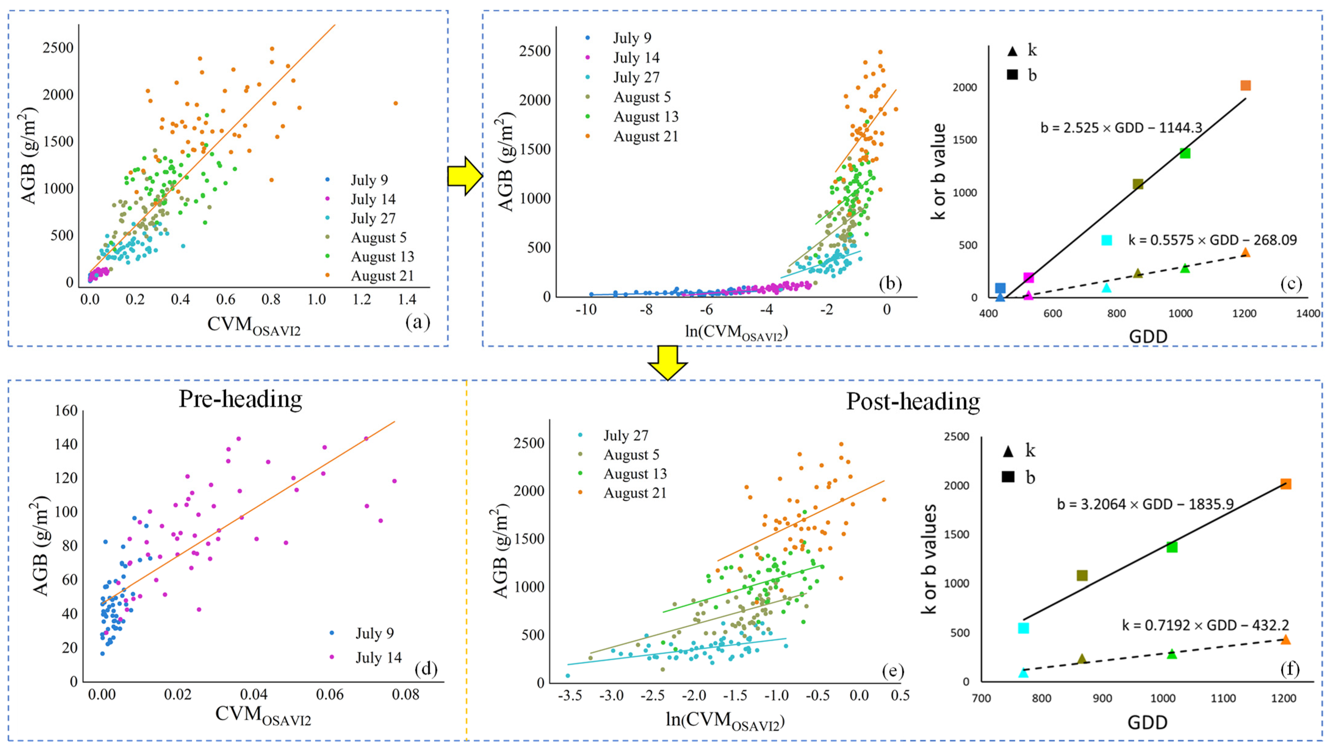
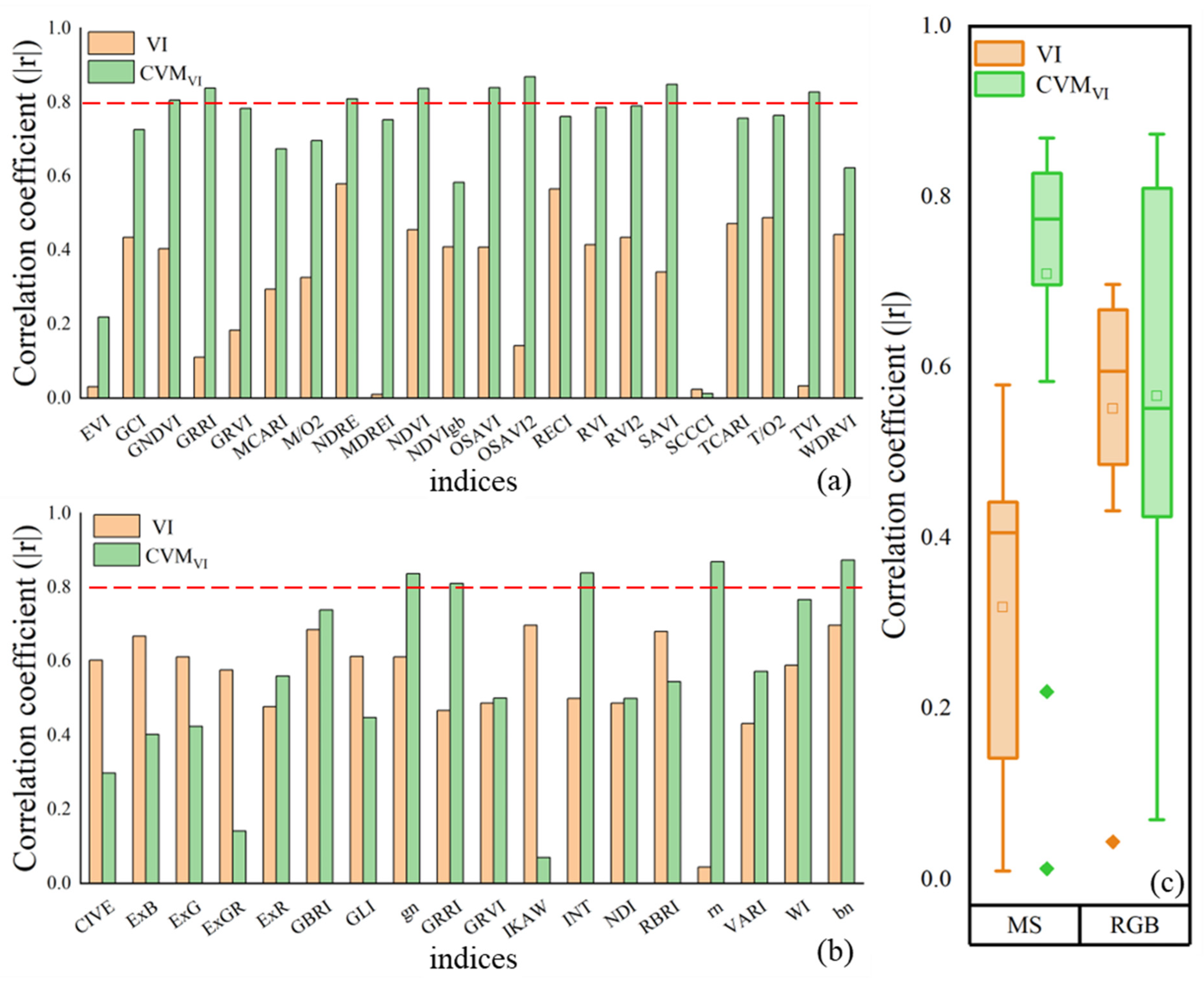
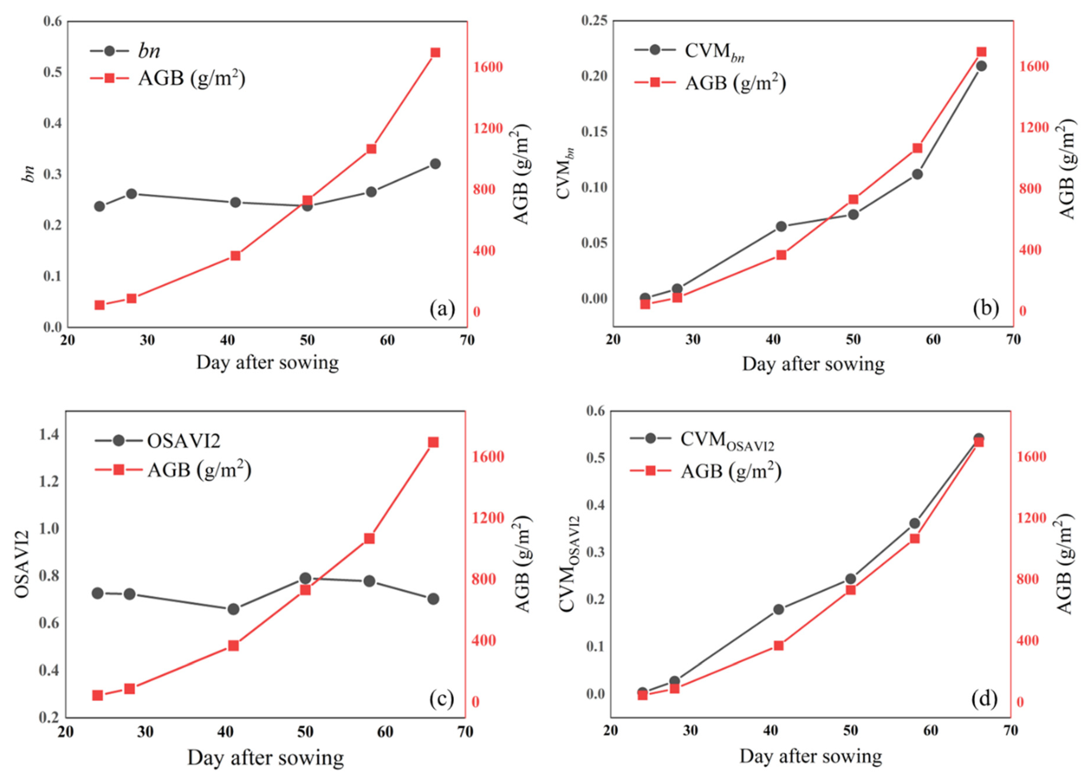
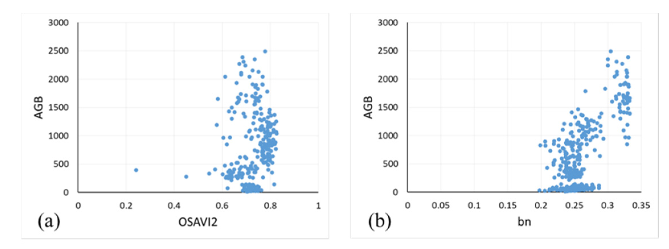
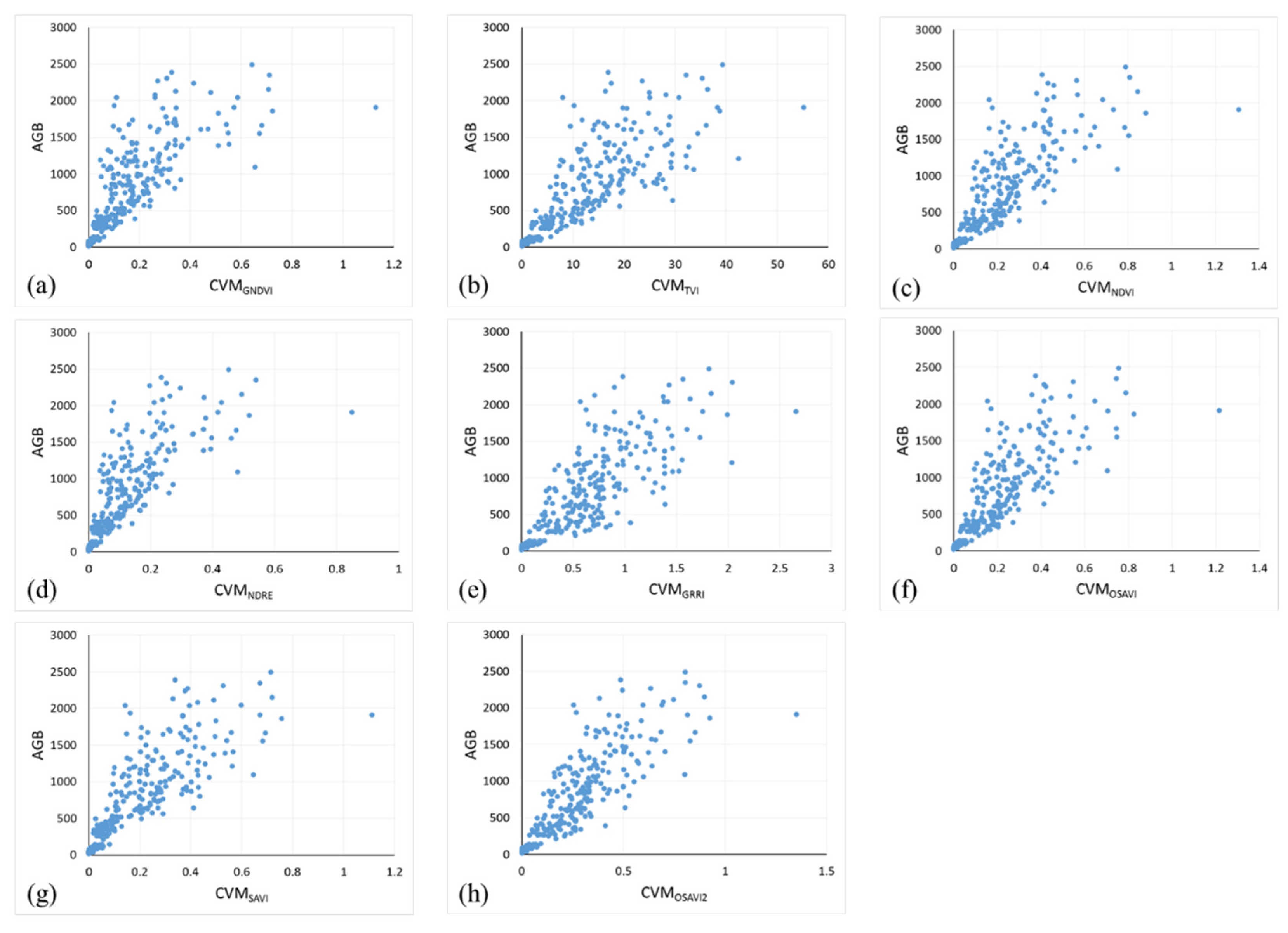
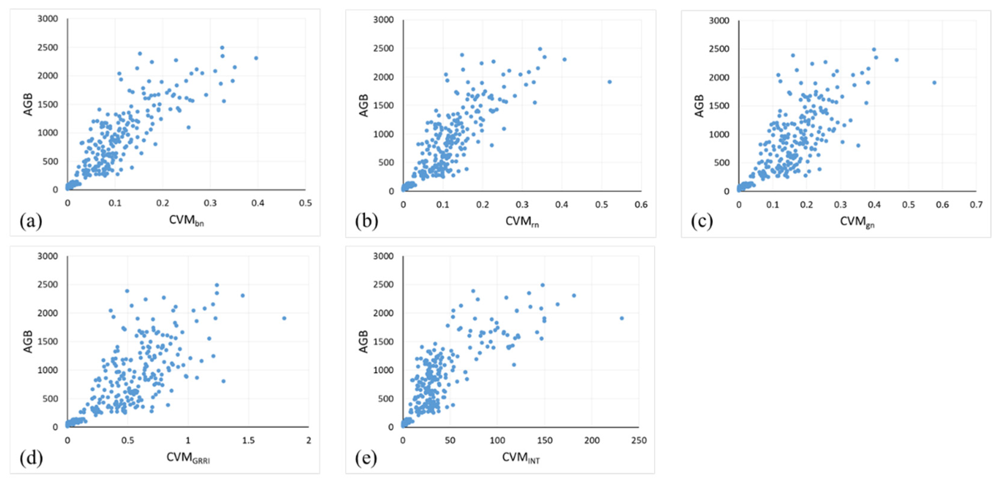
3.1. Correlation Analysis between VI, CVMVI, and AGB

The MS_VI with the highest correlation with AGB was NDRE, with a correlation coefficient of 0.58 (Figure 5a), while the RGB_VI with the highest correlation with AGB was bn, with a correlation coefficient of 0.7 (Figure 5b). Scatterplots of OSAVI2 and bn versus AGB were included in Figure A1 in the Appendix A. As can be seen from Figure 5c, the correlation between MS_VI and AGB was basically lower than 0.6, while the RGB_VI was higher. The average value of the correlation between RGB_VI and AGB was about 0.2 higher than MS_VI. Nevertheless, there was one RGB_VI (i.e., rn) with significantly lower correlation to AGB than the other RGB_VI, which was shown as an outlier in the boxplot (orange dot in Figure 5c).
CVMVI, which combined VI and CHM, showed an overall higher correlation than VI. The MS_CVMVI with the highest correlation with AGB was CVMOSAVI2, with a correlation coefficient of 0.87 (Figure 5a), while the RGB_CVMVI with the highest correlation with AGB was CVMbn, also with a correlation coefficient of 0.87 (Figure 5b). It was generally believed that, when the absolute value of correlation coefficient |r| was greater than or equal to 0.8, there was a strong correlation between the two variables [55]. In MS_CVMVI, there were eight indices with correlation coefficient |r| over 0.8. In the RGB_CVMVI, the correlation coefficient of only five indices exceeded 0.8. The scatter plots of MS_CVMVI and RGB_CVMVI versus AGB were shown in the Figure A2 and Figure A3, respectively. As can be seen from Figure 5c, the average RGB_CVMVI was less than 0.6, while that of MS_CVMVI was close to 0.8, and the difference between the two was about 0.2. Nevertheless, two MS_CVMVI indices (i.e., CVMEVI and CVMSCCCI) had significantly lower correlation to AGB than the other MS_CVMVI, which were shown as outliers in the boxplot (green dots in Figure 5c).
According to the results of correlation analysis, MS_NDRE and RGB_bn were used as input indicators of the CBA method, and MS_CVMOSAVI2 and RGB_CVMbn were used as input indicators for both iCBA and iCBA-PF.
To better understand the correlation between VI, CVMVI, and AGB, we compared the temporal change in different indices with that of AGB in the whole growing season, using bn, OSAVI2, and their corresponding CVMVI as examples (Figure 6). The average VI, CVMVI, and AGB of all the 56 plots were shown on the vertical axes. The two VIs were almost constant throughout the growing season, while AGB was continuously increasing (Figure 6a,c). In contrast, the temporal trend of CVMVI was similar to that of AGB as a whole (Figure 6b,d).

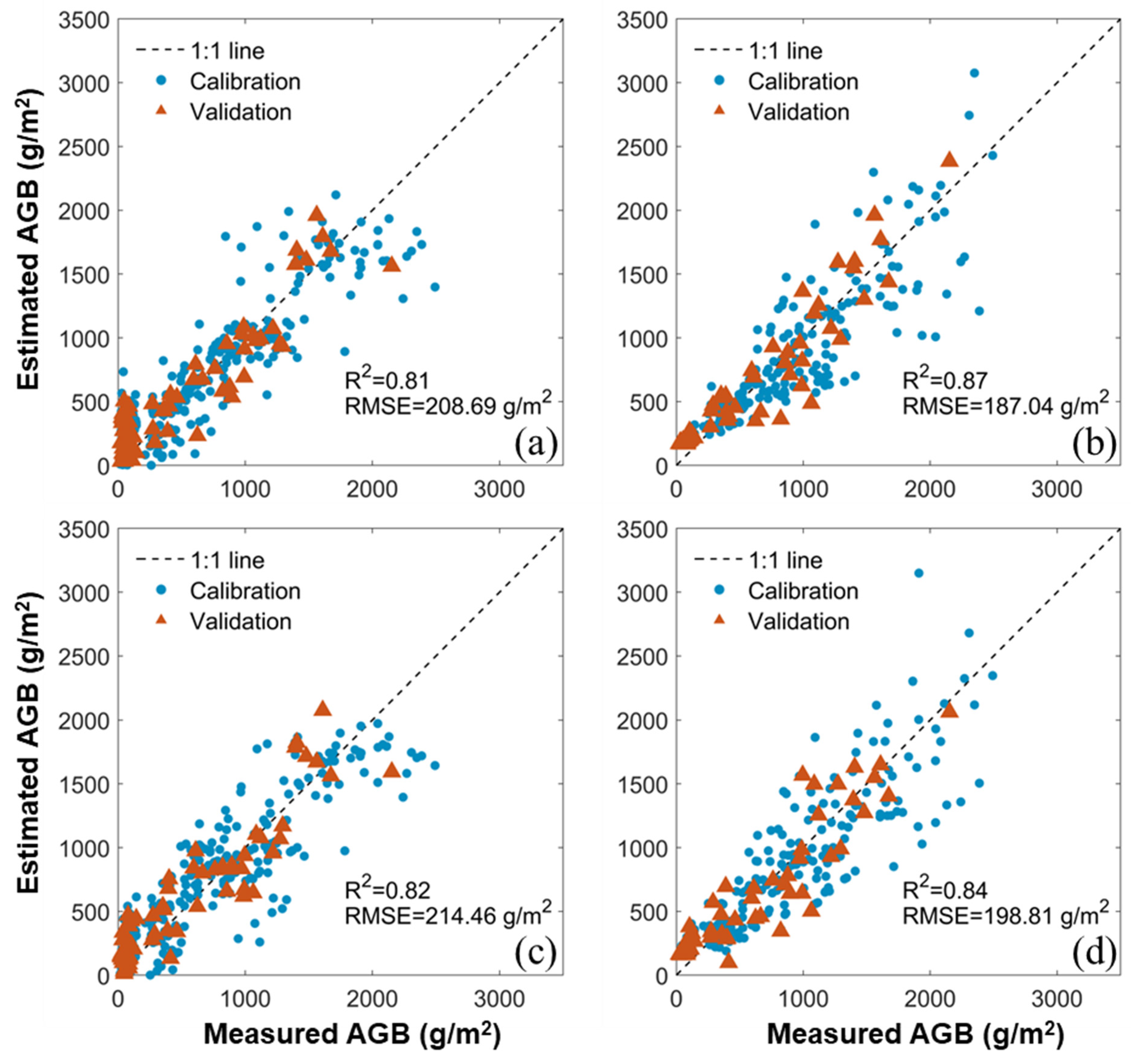
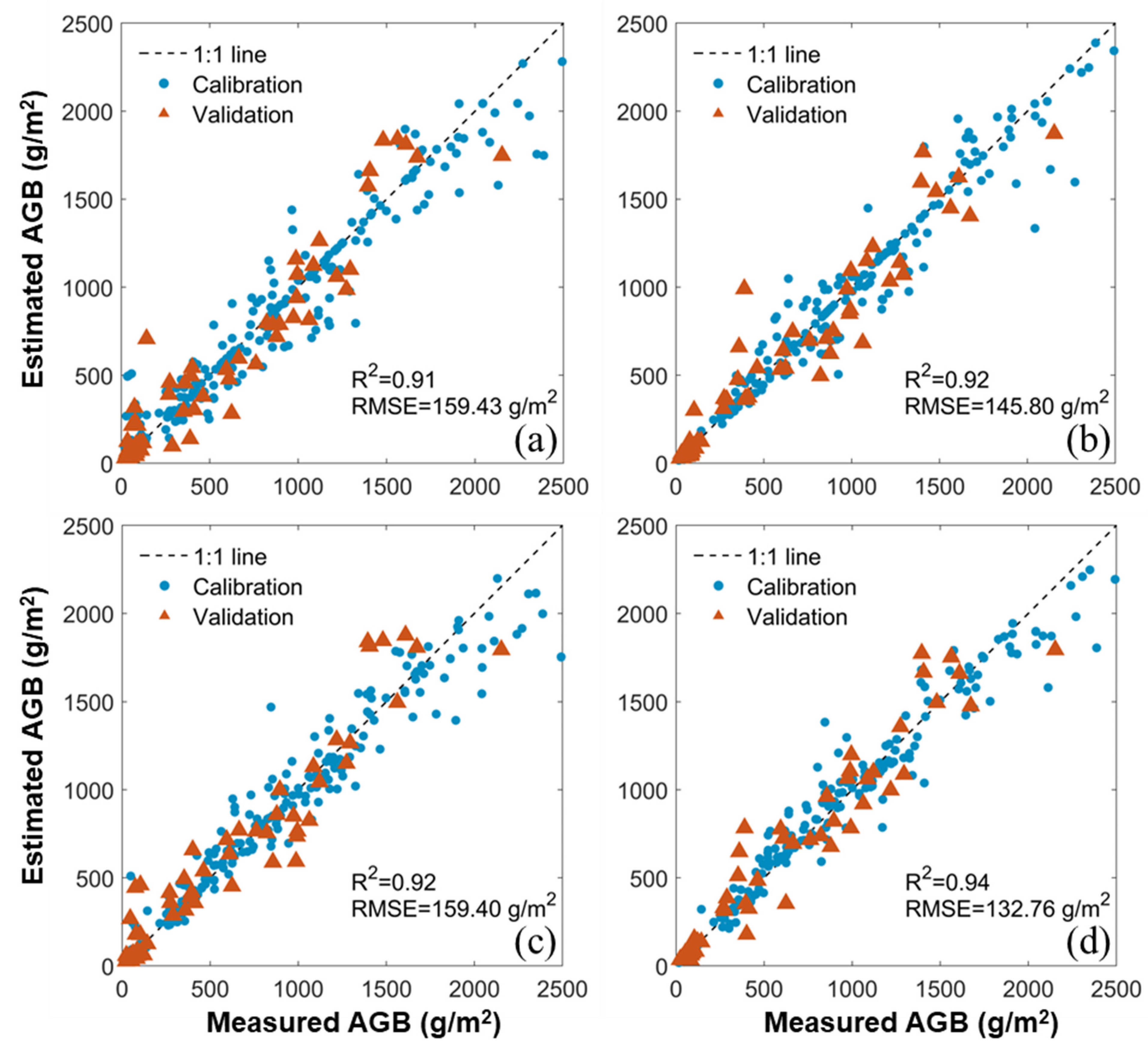
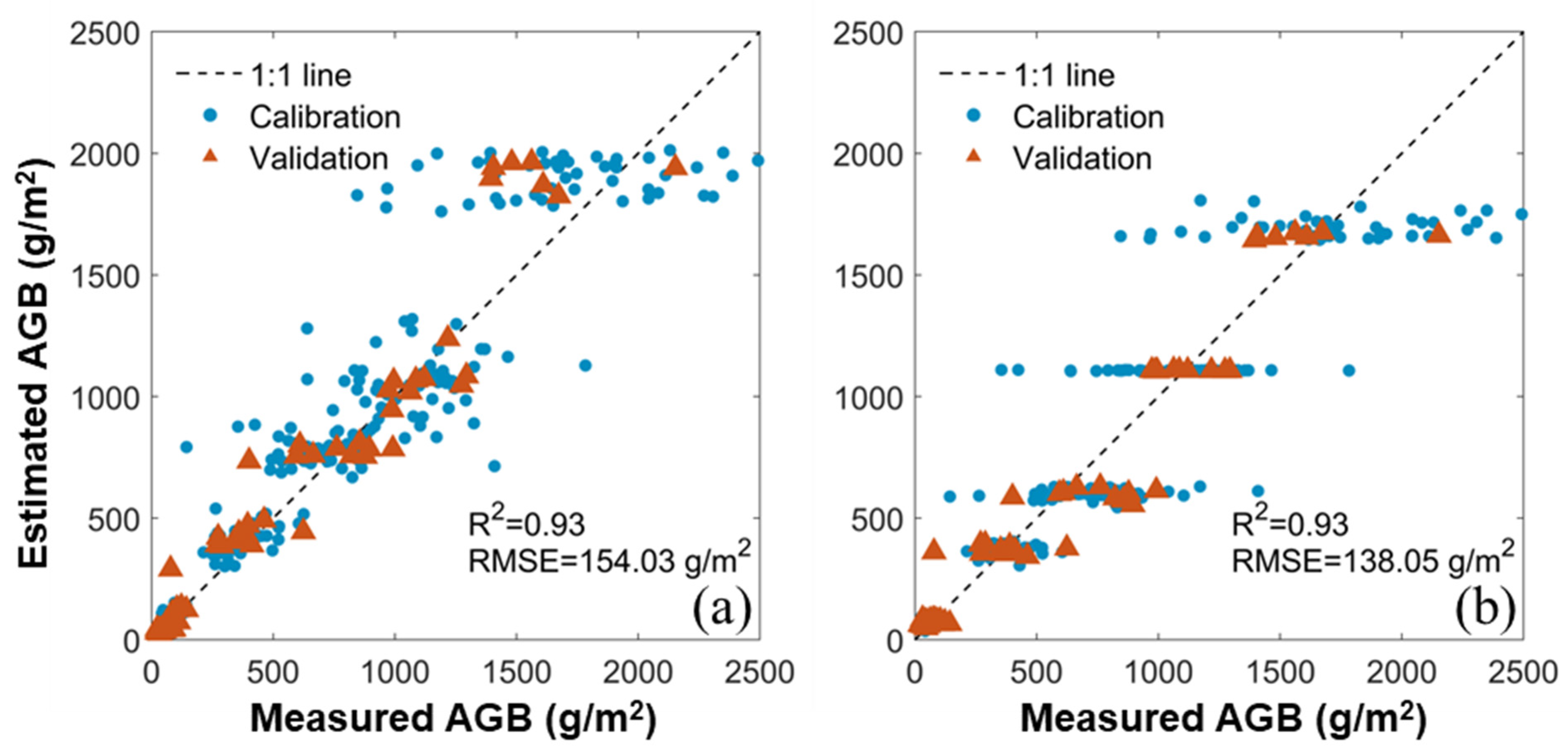
3.2. Estimation of AGB with Benchmark Methods

Figure 7, Figure 8 and Figure 9 were the results of maize AGB estimation by MLR, RFR, and CBA, respectively. In the MLR method, the difference between the results of VI and CVMVI was evident. Specifically, regardless of data source (MS_VI or RGB_VI), AGB was overestimated at the pre-heading stage. The overestimation in CVMVI at the pre-heading stage was alleviated, although not eliminated. The difference between the estimation results using VI and CVMVI of MS (Figure 7c versus Figure 7d) was smaller than that of RGB (Figure 7a versus Figure 7b). There was little difference between the estimation results of the two CVMVI (Figure 7b versus Figure 7d), with the RGB_CVMVI estimates (R2 = 0.87, RMSE = 187.04 g/m2) slightly more accurate.
As shown in Figure 8, the AGB estimation results of the RFR method with each type of indicator as input variables were underestimated at the R4 stage, while only MS_VI and RGB_VI were overestimated at the pre-heading stage. AGB was slightly underestimated at the R4 stage (with high AGB) with VIs as the input (Figure 8a,c), which was lightened when CVMVI were the input (Figure 8b,d). The most accurate estimation result was achieved based on MS_CVMVI among all indicators, with the highest R2 and the lowest RMSE (R2 = 0.94, RMSE = 132.76 g/m2) (Figure 8d). The accuracy of CVMVI estimation results was higher than the VI, which was the same as the MLR.
The k and b of GDD fitting were shown in Table 3. The coefficients in models for b were very small in some cases. This is because b was fitted as an exponential or power function, and GDD ranged from 400 to 1300. There would be a small factor to inhibit the explosive growth of b when the GDD value was relatively large. The results of estimating maize AGB at the six growth stages by the CBA method with MS_VI and RGB_VI were shown in Figure 9. The results of estimating maize AGB with bn (R2 = 0.93, RMSE = 138.05 g/m2, Figure 9b) were more accurate than with NDRE (R2 = 0.93, RMSE = 154.03 g/m2, Figure 9a). The results of the CBA method for estimating AGB had a clear boundary between different growth stages, especially in the RGB_VI estimates. Compared with the results of MLR and RFR, CBA had much less underestimation at the pre-heading stage. Although the estimation of maize AGB using CBA did not appear to be obviously underestimated at R4 stages, the closer to the harvest stage, the more dispersed the estimation results, which was one of the reasons for the estimation errors.

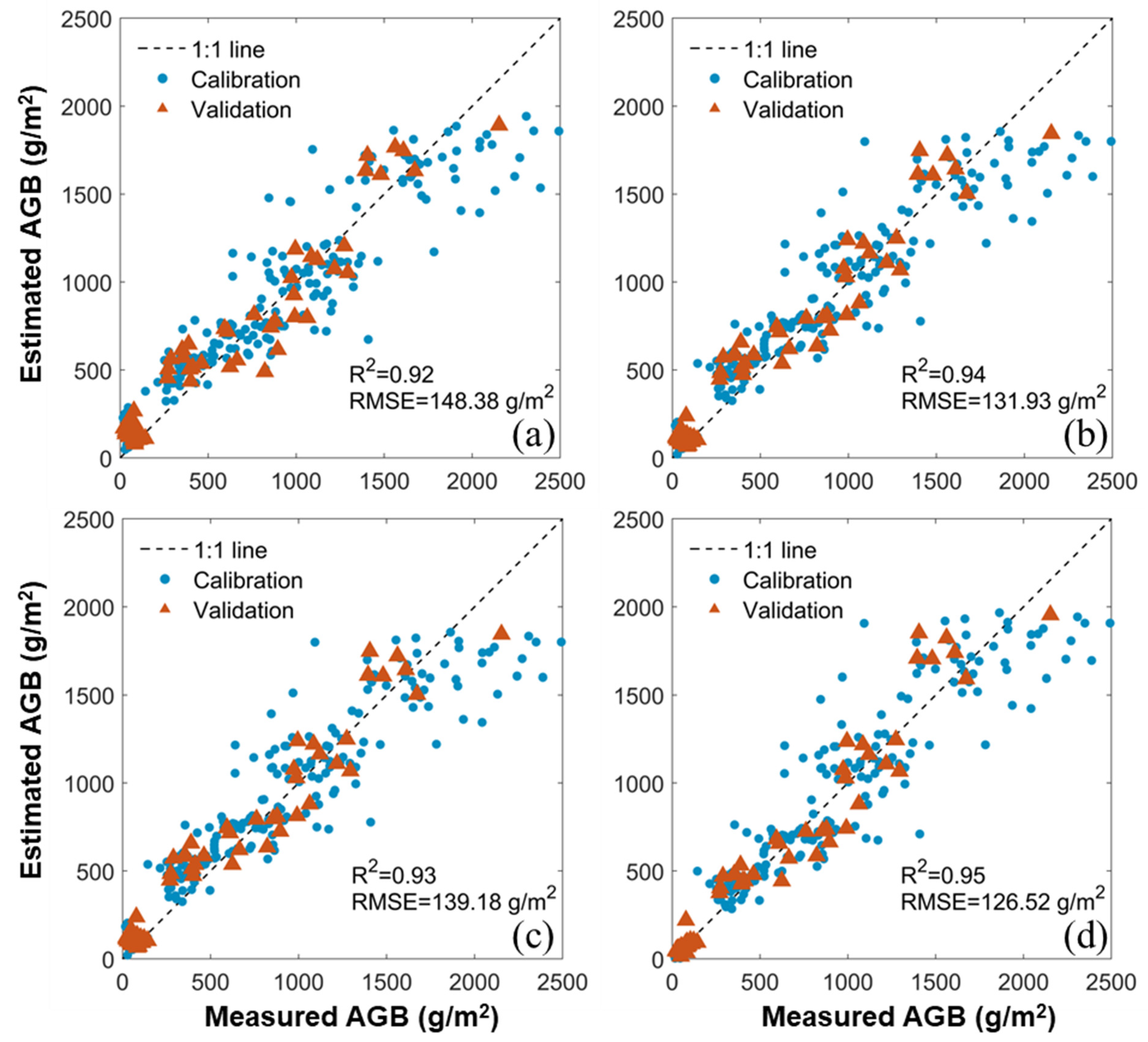
3.3. Estimation of AGB by iCBA and iCBA-PF

In the iCBA and iCBA-PF methods, k and b were all fitted with linear equations (Table 4). The results of estimating maize AGB using iCBA and iCBA-PF were shown in Figure 10. Regardless of MS or RGB, R2 was higher than 0.9 for all estimates and RMSE was less than 150 g/m2. The best estimation was the iCBA-PF method based on MS_CVMVI, with R2 of 0.95 and RMSE of 126.52 g/m2. Whether MS or RGB images, iCBA overestimated AGB at the pre-heading stages. The iCBA-PF method lessened this problem by fitting a separate simple linear equation at the pre-heading stage. Both methods improved the overall estimation accuracy of maize AGB for the whole growing season.

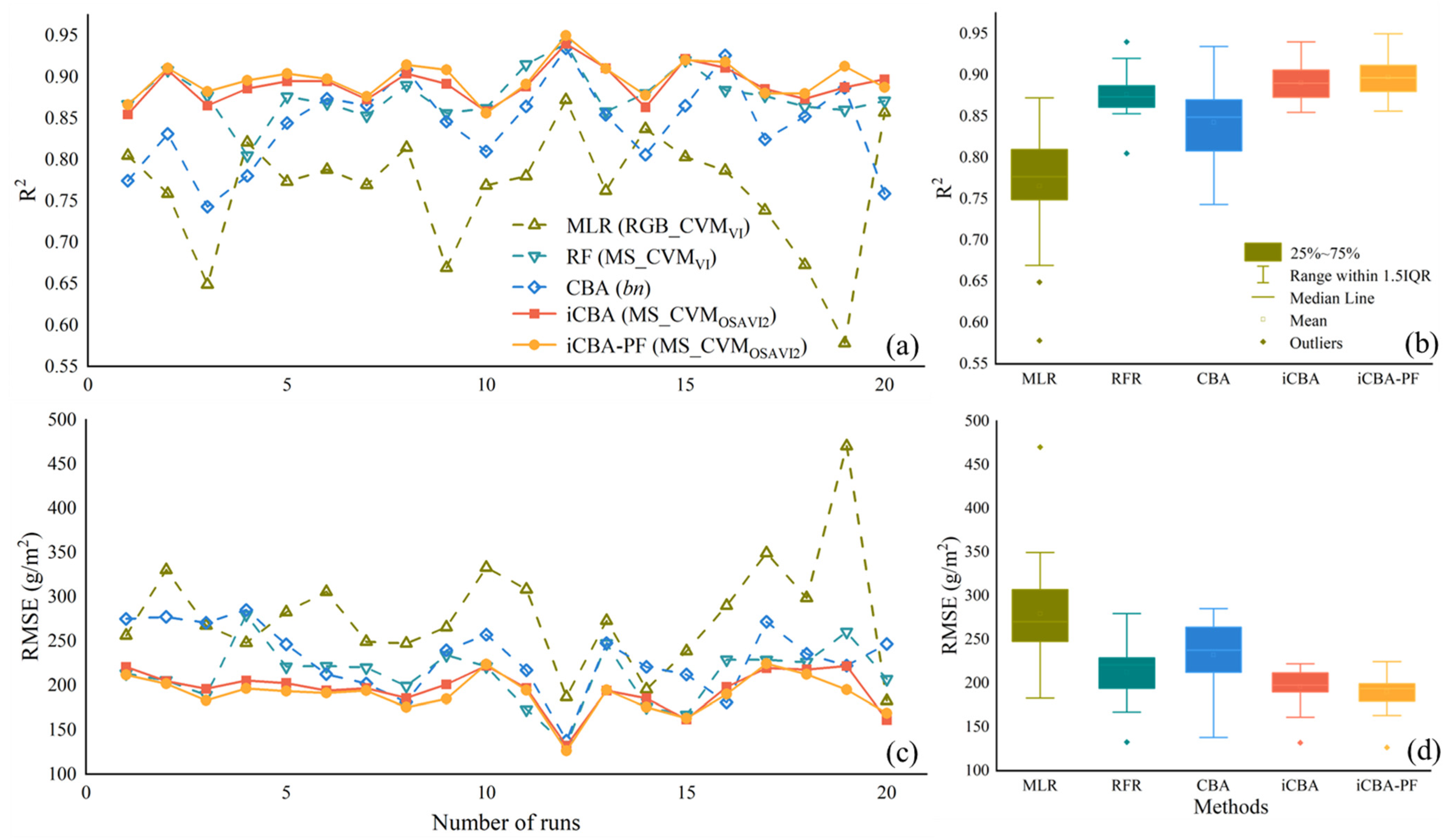
3.4. Comparison between the Benchmark and New Methods

The AGB estimation accuracy of all the above models were summarized in Table 5. The iCBA-PF method was the most accurate, with the highest R2 and lowest RMSE. For each method, two or four models were constructed depending on the type of input variable. The most accurate model using each method was marked in bold in Table 5. The optimal input indicators for MLR, RFR, CBA, iCBA, and iCBA-PF methods were all RGB_CVMVI, all MS_CVMVI, RGB_bn, MS_CVMOSAVI2, and MS_CVMOSAVI2, respectively. These optimal input indicators were used in the following method robustness evaluation.
The accuracy of the 20 runs of the five methods is shown in Figure 11. The results of R2 and RMSE of the validation set are shown in Figure 11a,c, and are further summarized in the boxplots (Figure 11b,d). Maize AGB estimated by MLR was significantly worse than those of the other four methods. The MLR method was the least accurate and robust of the five methods, followed by the CBA method. The accuracy of iCBA-PF, iCBA, and RFR methods were higher than MLR and CBA, but the robustness of RFR methods were slightly lower (accuracy variation was larger) than iCBA-PF and iCBA.
We further summarized the average accuracy (mean) and standard deviation (SD) of the 20 runs in Table 6. According to the 20 runs, the iCBA-PF method was the best maize AGB estimation method among the five methods. The average R2 of iCBA-PF was the highest and the average RMSE was the lowest, while the SD of both R2 and RMSE was the smallest (Table 6). Moreover, the paired t-test showed that the difference between iCBA-PF and the other four methods was statistically significant (p < 0.01).
By applying the most accurate model, i.e., the iCBA-PF method based on MS_CVMOSAVI2, we created the maize AGB maps (Figure 12). Each map was generated using the MS image and LiDAR point cloud collected on the corresponding date, details of which could be found in Table 1. The spatial distribution of maize AGB can be observed. Differences among maize varieties and different densities were also discerned. For example, the AGB of Zhengdan 958 (M2, black rectangles in Figure 12f) increased with increasing density (the planting density increases from left to the right). Differences in time were also evident in all plots. Moreover, the AGB values of bare soil (e.g., roads between plots) were close to 0 in each period, which also indicated that this method was suitable for the estimation of maize AGB.

4. Discussion

A new method for estimating maize AGB, iCBA-PF, was proposed in this paper by improving the selection of indicators, analysis methods, and grouping of maize growth stages. In indicator selection, CVMVI was used instead of VI, which combines 3D structure information with spectral information. Methodologically, the CBA method was applied to maize and improved to develop the iCBA method. On the grouping of growth stages, the growth stages were further divided into pre-heading and post-heading stages and modeled separately, which not only improved the accuracy of the method estimation, but also increased the efficiency. Experiments showed that the proposed iCBA-PF method was significantly more accurate than the existing methods in estimating maize AGB. We anticipate that iCBA-PF could be applied to other crops that have a heading stage, although experiments need to be conducted to verify this.

4.1. Comparison of MS and RGB Data in Different Methods

Optical images, especially MS and RGB images, are widely used for crop AGB estimation [14,56,57]. It is generally believed that RGB imagery has the advantages of low cost and high accuracy in the study of indicator estimation by remote sensing methods [58], while the advantages of MS imagery are mainly reflected in its RE and NIR bands which are more sensitive to vegetation.
The correlations of RGB_VI to AGB were stronger than those of MS_VI, which is consistent with previous studies [3,7,11]. Although MS_VI contains more spectral information, the RGB images in this study have much higher spatial resolution than the MS images. The differences in spatial resolution might be the main reason for the lower correlation between the MS_VI and AGB.
However, the correlation between MS_CVMVI and AGB was higher than that of RGB_CVMVI (Figure 5). The MS_CVMVI having strong correlation with AGB (|r| > 0.8) were mostly calculated with the NIR band, especially those in the normalized difference format. Maimaitijiang et al. [15] used RGB_CVMVI to estimate soybean AGB and found that CVMGRRI was the most relevant coefficient. Our results also confirmed that CVMGRRI was strongly correlated to AGB, whether it is calculated using MS or RGB data. Therefore, we infer that CVMGRRI is a good indicator when used to estimate the AGB of other crops.
The performance of these indices in AGB estimation was different from the correlation analysis. For example, although RGB_VI had higher correlation with AGB, the estimated AGB was not always more accurate than MS_VI, depending on which of the five AGB estimation methods were used. In this study, RGB factors were more accurate in MLR and CBA to estimate maize AGB, while MS factors were more accurate in the other methods (Table 5). Nevertheless, the accuracy difference between models with RGB and MS factors was not substantial, with R2 difference up to 0.03 (MLR with RGB_CVMVI vs MLR with MS_CVMVI) and RMSE difference less than 15.98 g/m2 (CBA with RGB_NDRE vs CBA with MS_bn).

4.2. Performance Comparison between VI and CVMVI of Two Sensors

Both MLR and RFR methods used VI and CVMVI to estimate maize AGB. The results of both methods showed that CVMVI had higher accuracy than VI, which was reflected in the lower RMSE and higher R2 (Table 5). The difference between CBA and iCBA mainly lies in the use of VI and CVMVI indicators. By replacing VI with CVMVI, the accuracy and robustness of the iCBA method (R2 = 0.89 ± 0.02, RMSE = 195.85 ± 22.28) both exceeded CBA (R2 = 0.84 ± 0.05, RMSE = 231.94 ± 36.93), as shown in Figure 11 and Table 6.
The comparison between the temporal trends of indices and AGB in the whole growing season (Figure 6) gave us some idea about why AGB was estimated with higher accuracy by CVMVI than by VI. While the VIs were almost constant throughout the growing season, both AGB and CVMVI had continuously increasing trends. This might be the reason for the high correlation between CVMVI and AGB. In addition, it also explains why VI overestimated AGB at early growth stage and underestimated AGB at late growth stage more severely than CVMVI.

4.3. Performance Comparison between New Methods and Benchmark Methods

Compared with the other methods, the iCBA-PF method had the highest accuracy and robustness in estimating maize AGB. The CBA method performed well in the study of estimating the AGB of winter wheat [20]. In this study, we used it to estimate the AGB of maize and found that the accuracy and robustness were greatly improved by replacing VI with CVMVI and applying a logarithmic conversion. Furthermore, by separating the pre- and post-heading stages, the iCBA-PF method achieved even higher accuracy. It was mainly reflected in the fact that there was almost no overestimation in its early stage. Although the problem of underestimation at the R4 stage remained unsolved, the overall AGB estimation accuracy in the whole growing season was improved. The stability of the iCBA-PF method was outstanding, which might be due to the use of CVMVI indicators that are more similar to the trend of AGB over the whole reproductive period (Figure 6).
Previous studies [19,59] used different methods to estimate the AGB of crops over the whole growing season and at different growth stages, and reached the same conclusion: the later the growth stage, the lower the accuracy of crop AGB estimation, and the accuracy of AGB estimation at the post-heading stage was generally lower than that at the whole growth stage. In this study, we take advantage of this finding to propose the iCBA-PF method, which first models separately the AGB at the pre- and post-heading stages and then combines them to obtain the complete AGB dataset. This approach proved effective, as evidenced by the higher accuracy and robustness of iCBA-PF than that of iCBA.

4.4. Limitation and Future Work

On the basis of previous studies, we proposed a method suitable for maize AGB estimation, and verified its accuracy and stability. However, it is uncertain whether this method is suitable for AGB estimation of other crops. We believe the crops that have a heading stage and the canopy volumn still changed at post-heading stage are suitable for estimating AGB using our method. Nevertheless, it is necessary to verify the applicability of the method on other crops in the future.
Although the new method proposed by us weakens the problem of underestimation of AGB at the R4 stage to a certain extent, the closer the harvest stage was, the more discrete the estimation result was. Part of the reason might be that the time difference between the acquisition of UAV and the ground truth was too long at the reproductive growth stage (e.g., UAV data on August 8 were paired with field data on August 13). In the future, we will conduct in-depth research and make improvements on this problem.

5. Conclusions

In this study, we proposed two new methods, iCBA and iCBA-PF, for AGB estimation. VI and CVMVI based on different data sources (MS and RGB) were calculated. AGB was estimated by three benchmark methods (MLR, RFR, CBA) and the two new methods (iCBA, iCBA-PF). The advantages and disadvantages between the iCBA-PF method and the benchmark methods were analyzed. Specific conclusions are as follows:
We found that RGB_VI had a higher correlation with maize AGB than MS_VI through correlation analysis, which was consistent with previous studies. However, the performance of MS data in AGB estimation was generally better than RGB data. On the other hand, RGB had a great advantage of price and spatial resolution. Hence, we recommend that you consider the balance of cost and accuracy when selecting the data source.
In the comparison of indicators, compared with VI, CVMVI had higher correlation with AGB and higher estimation accuracy regardless of method. We found that the temporal change trend of CVMVI and AGB during the whole growing season was more similar than VI, and might be a good substitute of VI in the future AGB estimation research.
Our proposed iCBA-PF method had the highest accuracy and the best robustness in estimating AGB among the selected methods. The accuracy improvement was statistically significant. The better performance of the iCBA-PF method over iCBA without separating growth stages also proved that modeling AGB at the pre-heading stage and post-heading stage separately was higher-performance than directly modeling the whole growing season.
Traditional field management mainly depends on the experience of agronomic experts. The accurate estimation of crop AGB at different growth stages helps agricultural managers to get a quantitative idea about the growth status of their crops. The AGB estimation approach with UAV remote sensing proposed in this study is highly efficient, non-destructive, and labor-saving. Moreover, the findings of this paper provide theoretical and technical support to the farmers regarding which sensors to purchase, how to plan flights, and how to process the data to monitor crop AGB.

Author Contributions

Methodology, data curation, conceptualization, formal analysis, and writing (original draft preparation), L.M.; conceptualization, validation, and writing (review and editing), D.Y.; data curation, M.C., S.L., Y.B., Y.L. (Yadong Liu), X.J. and F.N.; software, Y.L. (Yuan Liu) and Y.S.; resources, H.L.; funding acquisition, writing (review and editing), and conceptualization, X.J. All authors have read and agreed to the published version of the manuscript.

Funding

This research was supported by Central Public-interest Scientific Institution Basal Research Fund for Chinese Academy of Agricultural Sciences (Y2022XK22, Y2020YJ07), National Natural Science Foundation of China (42071426, 51922072, 51779161, 51009101), Key Cultivation Program of Xinjiang Academy of Agricultural Sciences (xjkcpy-2020003), the National Key Research and Development Program of China (2021YFD1201602), Research and application of key technologies of smart brain for farm decision-making platform (2021ZXJ05A03), the Agricultural Science and Technology Innovation Program of the Chinese Academy of Agricultural Sciences, Hainan Yazhou Bay Seed Lab (JBGS + B21HJ0221), and Nanfan special project, CAAS (YJTCY01, YBXM01).

Data Availability Statement

Data are available upon reasonable request; please Email jinxiuliang@caas.cn if you need the data.

Conflicts of Interest

The authors declare no conflict of interest.

Appendix A

Figure A1. Scatterplot of AGB against VIs. (a) The MS_VI with the strongest correlation to AGB: OSAVI2; (b) The RGB_VI with the strongest correlation to AGB: bn.
Drones 07 00254 g0a1
Figure A2. Scatterplot of AGB against the eight MS_CVMVI with strong correlation to AGB (|r| > 0.8). (a) CVMGNDVI; (b) CVMTVI; (c) CVMNDVI; (d) CVMNDRE; (e) CVMGRRI; (f) CVMOSAVI; (g) CVMSAVI; (h) CVMOSAVI2.
Drones 07 00254 g0a2
Figure A3. Scatterplot of AGB against the five RGB_CVMVI with strong correlation to AGB (|r| > 0.8). (a) CVMbn; (b) CVMrn; (c) CVMgn; (d) CVMGRRI; (e) CVMINT.
Drones 07 00254 g0a3

References

  1. Shiferaw, B.; Prasanna, B.M.; Hellin, J.; Bänziger, M. Crops that feed the world 6. Past successes and future challenges to the role played by maize in global food security. Food Secur. 2011, 3, 307–327. [Google Scholar] [CrossRef] [Green Version]
  2. Jin, X.; Ma, J.; Wen, Z.; Song, K. Estimation of Maize Residue Cover Using Landsat-8 OLI Image Spectral Information and Textural Features. Remote Sens. 2015, 7, 14559–14575. [Google Scholar] [CrossRef] [Green Version]
  3. Cen, H.; Wan, L.; Zhu, J.; Li, Y.; Li, X.; Zhu, Y.; Weng, H.; Wu, W.; Yin, W.; Xu, C.; et al. Dynamic monitoring of biomass of rice under different nitrogen treatments using a lightweight UAV with dual image-frame snapshot cameras. Plant Methods 2019, 15, 32. [Google Scholar] [CrossRef]
  4. Niu, Y.; Zhang, L.; Zhang, H.; Han, W.; Peng, X. Estimating Above-Ground Biomass of Maize Using Features Derived from UAV-Based RGB Imagery. Remote Sens. 2019, 11, 1261. [Google Scholar] [CrossRef] [Green Version]
  5. Yue, J.; Yang, G.; Tian, Q.; Feng, H.; Xu, K.; Zhou, C. Estimate of winter-wheat above-ground biomass based on UAV ultrahigh-ground-resolution image textures and vegetation indices. ISPRS J. Photogramm. Remote Sens. 2019, 150, 226–244. [Google Scholar] [CrossRef]
  6. Maimaitijiang, M.; Ghulam, A.; Sidike, P.; Hartling, S.; Maimaitiyiming, M.; Peterson, K.; Shavers, E.; Fishman, J.; Peterson, J.; Kadam, S.; et al. Unmanned Aerial System (UAS)-based phenotyping of soybean using multi-sensor data fusion and extreme learning machine. ISPRS J. Photogramm. Remote Sens. 2017, 134, 43–58. [Google Scholar] [CrossRef]
  7. Han, L.; Yang, G.; Dai, H.; Xu, B.; Yang, H.; Feng, H.; Li, Z.; Yang, X. Modeling maize above-ground biomass based on machine learning approaches using UAV remote-sensing data. Plant Methods 2019, 15, 10. [Google Scholar] [CrossRef] [Green Version]
  8. Moeckel, T.; Dayananda, S.; Nidamanuri, R.; Nautiyal, S.; Hanumaiah, N.; Buerkert, A.; Wachendorf, M. Estimation of Vegetable Crop Parameter by Multi-temporal UAV-Borne Images. Remote Sens. 2018, 10, 805. [Google Scholar] [CrossRef] [Green Version]
  9. Chen, Q. Modeling aboveground tree woody biomass using national-scale allometric methods and airborne lidar. ISPRS J. Photogramm. Remote Sens. 2015, 106, 95–106. [Google Scholar] [CrossRef]
  10. Wang, G.; Liu, S.; Liu, T.; Fu, Z.; Yu, J.; Xue, B. Modelling above-ground biomass based on vegetation indexes: A modified approach for biomass estimation in semi-arid grasslands. Int. J. Remote Sens. 2018, 40, 3835–3854. [Google Scholar] [CrossRef]
  11. Roth, L.; Streit, B. Predicting cover crop biomass by lightweight UAS-based RGB and NIR photography: An applied photogrammetric approach. Precis. Agric. 2017, 19, 93–114. [Google Scholar] [CrossRef] [Green Version]
  12. Guo, Y.; Chen, S.; Li, X.; Cunha, M.; Jayavelu, S.; Cammarano, D.; Fu, Y. Machine learning-based approaches for predicting SPAD values of maize using multi-spectral images. Remote Sens. 2022, 14, 1337. [Google Scholar] [CrossRef]
  13. Li, P.; Zhang, X.; Wang, W.; Zheng, H.; Yao, X.; Tian, Y.; Zhu, Y.; Cao, W.; Chen, Q.; Cheng, T. Estimating aboveground and organ biomass of plant canopies across the entire season of rice growth with terrestrial laser scanning. Int. J. Appl. Earth Obs. Geoinf. 2020, 91, 102132. [Google Scholar] [CrossRef]
  14. Yue, J.; Feng, H.; Jin, X.; Yuan, H.; Li, Z.; Zhou, C.; Yang, G.; Tian, Q. A Comparison of Crop Parameters Estimation Using Images from UAV-Mounted Snapshot Hyperspectral Sensor and High-Definition Digital Camera. Remote Sens. 2018, 10, 1138. [Google Scholar] [CrossRef] [Green Version]
  15. Maimaitijiang, M.; Sagan, V.; Sidike, P.; Maimaitiyiming, M.; Hartling, S.; Peterson, K.T.; Maw, M.J.W.; Shakoor, N.; Mockler, T.; Fritschi, F.B. Vegetation Index Weighted Canopy Volume Model (CVMVI) for soybean biomass estimation from Unmanned Aerial System-based RGB imagery. ISPRS J. Photogramm. Remote Sens. 2019, 151, 27–41. [Google Scholar] [CrossRef]
  16. Li, W.; Niu, Z.; Chen, H.; Li, D.; Wu, M.; Zhao, W. Remote estimation of canopy height and aboveground biomass of maize using high-resolution stereo images from a low-cost unmanned aerial vehicle system. Ecol. Indic. 2016, 67, 637–648. [Google Scholar] [CrossRef]
  17. Xu, L.; Zhou, L.; Meng, R.; Zhao, F.; Lv, Z.; Xu, B.; Zeng, L.; Yu, X.; Peng, S. An improved approach to estimate ratoon rice aboveground biomass by integrating UAV-based spectral, textural and structural features. Precis. Agric. 2022, 23, 1276–1301. [Google Scholar] [CrossRef]
  18. Liu, Y.; Liu, S.; Li, J.; Guo, X.; Wang, S.; Lu, J. Estimating biomass of winter oilseed rape using vegetation indices and texture metrics derived from UAV multispectral images. Comput. Electron. Agric. 2019, 166, 105026. [Google Scholar] [CrossRef]
  19. Zheng, H.; Cheng, T.; Zhou, M.; Li, D.; Yao, X.; Tian, Y.; Cao, W.; Zhu, Y. Improved estimation of rice aboveground biomass combining textural and spectral analysis of UAV imagery. Precis. Agric. 2018, 20, 611–629. [Google Scholar] [CrossRef]
  20. Li, Z.; Zhao, Y.; Taylor, J.; Gaulton, R.; Jin, X.; Song, X.; Li, Z.; Meng, Y.; Chen, P.; Feng, H.; et al. Comparison and transferability of thermal, temporal and phenological-based in-season predictions of above-ground biomass in wheat crops from proximal crop reflectance data. Remote Sens. Environ. 2022, 273, 112967. [Google Scholar] [CrossRef]
  21. Liu, Y.; Nie, C.; Zhang, Z.; Wang, Z.; Ming, B.; Xue, J.; Yang, H.; Xu, H.; Meng, L.; Cui, N.; et al. Evaluating how lodging affects maize yield estimation based on UAV observations. Front. Plant Sci. 2022, 13, 979103. [Google Scholar] [CrossRef]
  22. Rouse, J.W., Jr.; Haas, R.H.; Schell, J.A.; Deering, D.W. Monitoring Vegetation Systems in the Great Plains with ERTS; NASA: Washington, DC, USA, 1974; Volume 1.
  23. Wang, F.M.; Huang, J.F.; Tang, Y.L.; Wang, X.Z. New Vegetation Index and Its Application in Estimating Leaf Area Index of Rice. Rice Sci. 2007, 14, 195–203. [Google Scholar] [CrossRef]
  24. Broge, N.H.; Leblanc, E. Comparing prediction power and stability of broadband and hyperspectral vegetation indices for estimation of green leaf area index and canopy chlorophyll density. Remote Sens. Environ. 2001, 76, 156–172. [Google Scholar] [CrossRef]
  25. Rondeaux, G.; Steven, M.; Baret, F. Optimization of soil-adjusted vegetation indices. Remote Sens. Environ. 1996, 55, 95–107. [Google Scholar] [CrossRef]
  26. Huete, A.R. A soil-adjusted vegetation index (SAVI). Remote Sens. Environ. 1988, 25, 295–309. [Google Scholar] [CrossRef]
  27. Mishra, S.; Mishra, D.R. Normalized difference chlorophyll index: A novel model for remote estimation of chlorophyll-a concentration in turbid productive waters. Remote Sens. Environ. 2012, 117, 394–406. [Google Scholar] [CrossRef]
  28. Xue, L.; Cao, W.; Luo, W.; Dai, T.; Yan, Z.J. Monitoring Leaf Nitrogen Status in Rice with Canopy Spectral Reflectance. Agron. J. 2004, 96, 135–142. [Google Scholar] [CrossRef]
  29. Huete, A.; Didan, K.; Miura, T.; Rodriguez, E.P.; Gao, X.; Ferreira, L.G. Overview of the radiometric and biophysical performance of the MODIS vegetation indices. Remote Sens. Environ. 2002, 83, 195–213. [Google Scholar] [CrossRef]
  30. Gitelson, A.; Vina, A.; Ciganda, V. Remote estimation of canopy chlorophyll content in crops. Geophys. Res. Lett. 2005, 32, L08403. [Google Scholar] [CrossRef] [Green Version]
  31. Tucker, C.J. Red and photographic infrared linear combinations for monitoring vegetation. Remote Sens. Environ. 1979, 8, 127–150. [Google Scholar] [CrossRef] [Green Version]
  32. Verrelst, J.; Schaepman, M.E.; Koetz, B.; Environment, M. Angular sensitivity analysis of vegetation indices derived from CHRIS/PROBA data. Remote Sens. Environ. 2008, 112, 2341–2353. [Google Scholar] [CrossRef]
  33. Gitelson, A.A.; Merzlyak, M.N. Remote estimation of chlorophyll content in higher plant leaves. Int. J. Remote Sens. 1997, 18, 2691–2697. [Google Scholar] [CrossRef]
  34. Muhammad, H.; Yang, M.; Awais, R.; Jin, X.; Xia, X.; Xiao, Y.; He, Z. Time-series multispectral indices from unmanned aerial vehicle imagery reveal senescence rate in bread wheat. Remote Sens. 2018, 10, 809. [Google Scholar]
  35. Raper, T.B.; Varco, J.J. Canopy-scale wavelength and vegetative index sensitivities to cotton growth parameters and nitrogen status. Precis. Agric. 2015, 16, 62–76. [Google Scholar] [CrossRef] [Green Version]
  36. Haboudane, D.; Miller, J.R.; Tremblay, N.; Zarco-Tejada, P.J.; Dextraze, L. Integrated narrow-band vegetation indices for prediction of crop chlorophyll content for application to precision agriculture. Remote Sens. Environ. 2002, 81, 416–426. [Google Scholar] [CrossRef]
  37. Daughtry, C.; Walthall, C.L.; Kim, M.S.; Colstoun, E.; McMurtrey Iii, J.E. Estimating Corn Leaf Chlorophyll Concentration from Leaf and Canopy Reflectance. Remote Sens. Environ. 2000, 74, 229–239. [Google Scholar] [CrossRef]
  38. Gamon, J.; Surfus, J. Assessing leaf pigment content with a reflectometer. New Phytol. 1999, 143, 105–117. [Google Scholar] [CrossRef]
  39. Kawashima, S.; Nakatani, M. An Algorithm for Estimating Chlorophyll Content in Leaves Using a Video Camera. Ann. Bot. 1998, 81, 49–54. [Google Scholar] [CrossRef] [Green Version]
  40. Ahmad, I.S.; Reid, J.F. Evaluation of Colour Representations for Maize Images. J. Agric. Eng. Res. 1996, 63, 185–195. [Google Scholar] [CrossRef]
  41. Woebbecke, D.M.; Meyer, G.E.; Bargen, K.V.; Mortensen, D.A. Plant species identification, size, and enumeration using machine vision techniques on near-binary images. SPIE Proc. Ser. 1993, 1836, 208–219. [Google Scholar]
  42. Woebbecke, D.M.; Meyer, G.E.; Bargen, K.V.; Mortensen, D.A. Color Indices for Weed Identification Under Various Soil, Residue, and Lighting Conditions. Trans. ASAE 1995, 38, 259–269. [Google Scholar] [CrossRef]
  43. Louhaichi, M.; Borman, M.M.; Johnson, D.E. Spatially Located Platform and Aerial Photography for Documentation of Grazing Impacts on Wheat. Geocarto Int. 2008, 16, 65–70. [Google Scholar] [CrossRef]
  44. Gitelson, A.A.; Kaufman, Y.J.; Stark, R.; Rundquist, D. Novel algorithms for remote estimation of vegetation fraction. Remote Sens. Environ. 2002, 80, 76–87. [Google Scholar] [CrossRef] [Green Version]
  45. Mao, W.; Wang, Y.; Wang, Y. Real-time Detection of Between-row Weeds Using Machine Vision. In Proceedings of the 2003 ASAE Annual Meeting, Las Vegas, NV, USA, 27–30 July 2003. [Google Scholar]
  46. Guijarro, M.; Pajares, G.; Riomoros, I.; Herrera, P.J.; Burgos-Artizzu, X.P.; Ribeiro, A. Automatic segmentation of relevant textures in agricultural images. Comput. Electron. Agric. 2011, 75, 75–83. [Google Scholar] [CrossRef] [Green Version]
  47. Duncanson, L.I.; Cook, B.D.; Hurtt, G.C.; Dubayah, R.O. An efficient, multi-layered crown delineation algorithm for mapping individual tree structure across multiple ecosystems. Remote Sens. Environ. 2014, 154, 378–386. [Google Scholar] [CrossRef]
  48. Hickey, S.; Callow, N.; Phinn, S.; Lovelock, C.; Duarte, C.M. Spatial complexities in aboveground carbon stocks of a semi-arid mangrove community: A remote sensing height-biomass-carbon approach. Estuar. Coast. Shelf Sci. 2018, 200, 194–201. [Google Scholar] [CrossRef] [Green Version]
  49. Yin, D.; Wang, L. Individual mangrove tree measurement using UAV-based LiDAR data: Possibilities and challenges. Remote Sens. Environ. 2019, 223, 34–49. [Google Scholar] [CrossRef]
  50. Ahmad, A.; Gilani, H.; Ahmad, S.R. Forest Aboveground Biomass Estimation and Mapping through High-Resolution Optical Satellite Imagery—A Literature Review. Forests 2021, 12, 914. [Google Scholar] [CrossRef]
  51. Jayathunga, S.; Owari, T.; Tsuyuki, S. Digital Aerial Photogrammetry for Uneven-Aged Forest Management: Assessing the Potential to Reconstruct Canopy Structure and Estimate Living Biomass. Remote Sens. 2019, 11, 338. [Google Scholar] [CrossRef] [Green Version]
  52. Wang, Z.; Wang, M.; Yin, X.; Zhang, H.; Chu, Q.; Wen, X.; Chen, F. Spatiotemporal characteristics of heat and rainfall changes in summer maize season under climate change in the North China Plain. Chin. J. Eco-Agric. 2015, 23, 473–481. [Google Scholar]
  53. Jin, X.; Li, Z.; Feng, H.; Ren, Z.; Li, S. Deep neural network algorithm for estimating maize biomass based on simulated Sentinel 2A vegetation indices and leaf area index. Crop J. 2020, 8, 87–97. [Google Scholar] [CrossRef]
  54. Ross, A.; Willson, V.L. Paired Samples T-Test. In Basic and Advanced Statistical Tests: Writing Results Sections and Creating Tables and Figures; SensePublishers: Rotterdam, The Netherlands, 2017; pp. 17–19. [Google Scholar]
  55. Li, Z.; Lu, D.; Gao, X. Analysis of correlation between hydration heat release and compressive strength for blended cement pastes. Constr. Build. Mater. 2020, 260, 120436. [Google Scholar] [CrossRef]
  56. Jin, X.; Yang, G.; Li, Z.; Xu, X.; Wang, J.; Lan, Y. Estimation of water productivity in winter wheat using the AquaCrop model with field hyperspectral data. Precis. Agric. 2016, 19, 1–17. [Google Scholar] [CrossRef]
  57. Bendig, J.; Yu, K.; Aasen, H.; Bolten, A.; Bennertz, S.; Broscheit, J.; Gnyp, M.L.; Bareth, G. Combining UAV-based plant height from crop surface models, visible, and near infrared vegetation indices for biomass monitoring in barley. Int. J. Appl. Earth Obs. Geoinf. 2015, 39, 79–87. [Google Scholar] [CrossRef]
  58. Jin, X.; Liu, S.; Baret, F.; Hemerlé, M.; Comar, A. Estimates of plant density of wheat crops at emergence from very low altitude UAV imagery. Remote Sens. Environ. 2017, 198, 105–114. [Google Scholar] [CrossRef] [Green Version]
  59. Zhang, Y.; Xia, C.; Zhang, X.; Cheng, X.; Feng, G.; Wang, Y.; Gao, Q. Estimating the maize biomass by crop height and narrowband vegetation indices derived from UAV-based hyperspectral images. Ecol. Indic. 2021, 129, 107985. [Google Scholar] [CrossRef]
Figure 1. The workflow of this study.
Drones 07 00254 g001
Figure 2. The geographical location of Henan Province in China (a), experiment site location (b), and specific experimental design (c).
Drones 07 00254 g002
Figure 3. Schematic diagram of field sampling. (a) Sampling time. The red boxes mark the maize growth stage at each sampling time. (b) Example of a plot before and after sampling. The orange box is the boundary of the plot.
Drones 07 00254 g003
Figure 4. Flowchart of the development of iCBA and iCBA-PF. (a) Scatterplot of CVMOSAVI2 and AGB in each sampling stage. (b) Linear regressions between ln(CVMOSAVI2) and AGB, grouped by sampling time. (c) Linear regression between k or b and GDD. (d) Linear regression between CVMOSAVI2 and AGB at the pre-heading stage. (e) Linear regression between ln(CVMOSAVI2) and AGB at the post-heading stage, grouped by sampling time. (f) Linear regression between k or b and GDD, at the post-heading stage.
Drones 07 00254 g004
Figure 5. Correlation analysis between the indicators and AGB. (a) Indicators from the MS data. (b) Indicators from the RGB data. (c) Comparison between the four types of indicators. The red dashed lines in (a,b) represent the correlation coefficient |r| equal to 0.8.
Drones 07 00254 g005
Figure 6. Time series of indicators and AGB in the maize growing season. (a) RGB_bn and AGB. (b) RGB_CVMbn and AGB. (c) MS_OSAVI2 and AGB. (d) MS_CVMOSAVI2 and AGB.
Drones 07 00254 g006
Figure 7. Estimated and measured maize AGB (g/m2) with MLR: (a) all RGB_VI; (b) all RGB_CVMVI; (c) all MS_VI; (d) all MS_CVMVI.
Drones 07 00254 g007
Figure 8. Estimated and measured maize AGB (g/m2) with RFR: (a) all RGB_VI; (b) all RGB_CVMVI; (c) all MS_VI; (d) all MS_CVMVI.
Drones 07 00254 g008
Figure 9. Estimated and measured maize AGB (g/m2) with CBA: (a) MS_NDRE; (b) RGB_bn.
Drones 07 00254 g009
Figure 10. Estimated and measured maize AGB (g/m2) with iCBA and iCBA-PF: (a) iCBA based on RGB_CVMbn; (b) iCBA-PF based on RGB_CVMbn; (c) iCBA based on MS_CVMOSAVI2; (d) iCBA-PF based on MS_CVMOSAVI2.
Drones 07 00254 g010
Figure 11. Maize AGB estimation accuracy from the five methods run 20 times. (a) R2 of the 20 runs of five methods. (b) R2 comparison of the five methods. (c) RMSE of the 20 runs of five methods. (d) RMSE comparison of the five methods.
Drones 07 00254 g011
Figure 12. AGB estimation based on iCBA-PF with MS_CVMOSAVI2: (a) 9 July; (b) 14 July; (c) 27 July; (d) 5 August; (e) 13 August; (f) 21 August.
Drones 07 00254 g012
Table 1. Specific information of the UAV data.
Date of Data AcquisitionRGBMSLiDAR
FA (m)SR (m)FA (m)SR (m)FA (m)SR (m)
9 July 2021200.00279200.018300.016
12 July 2021200.00219200.018300.014
26 July 2021200.00218200.018300.017
31 July 2021200.00346200.018300.025
8 August 2021700.00792700.050300.019
18 August 2021300.011401000.078300.019
Table 2. Definitions of the VIs extracted from orthorectified MS and RGB mosaics.
SensorSpectral IndicesDefinitionReference
MSNormalized difference vegetation index (NDVI)NDVI = (NIR − R)/(NIR + R)[22]
Green-normalized difference vegetation index (GNDVI)GNDVI = (NIR − G)/(NIR + G)[23]
Triangular vegetation index (TVI)TVI = 60 × (NIR − G) − 100 × (R − G)[24]
Optimized soil adjusted vegetation index (OSAVI)OSAVI = 1.16 × (NIR − R)/(NIR + R + 0.16)[25]
Soil-adjusted vegetation index (SAVI)SAVI = 1.5 × (NIR − R)/(NIR + R + 0.5)[26]
Ratio vegetation index (RVI)RVI = NIR/R[27]
Ratio vegetation index 2 (RVI2)RVI2 = NIR/G[28]
Enhanced vegetation index (EVI)EVI = 2.5 × (NIR − R)/(NIR + 6 × R − 7.5 × B + 1)[29]
Green chlorophyll index (GCI)GCI = (NIR/G) − 1[30]
Red-edge chlorophyll index (RECI) RECI = (NIR/RE) − 1[30]
Green–red vegetation index (GRVI)GRVI = (G − R)/(G + R)[31]
Normalized difference vegetation index 2 (NDVIgb)NDVIgb = (G − B)/(G + B)[32]
Normalized difference red-edge (NDRE)NDRE = (NIR − RE)/(NIR + RE)[33]
Normalized difference red-edge index (NDREI)NDREI = (RE − G)/(RE + G)[34]
Simplified canopy chlorophyll content index (SCCCI)SCCCI = NDRE/NDVI[35]
Optimized soil adjusted vegetation index 2 (OSAVI2)OSAVI2 = (NIR − R)/(NIR − R + 0.16)[25]
Modified chlorophyll absorption in reflectance index (MCARI)MCARI = [(RE − R) − 0.2 × (RE − G)] × (RE/R)[36]
Transformed chlorophyll absorption in reflectance index (TCARI)TCARI = 3 × [(RE − R) − 0.2 × (RE − G) × (RE/R)][36]
MCARI/OSAVI2 (M/O2)MCARI/OSAVI2[37]
TCARI/OSAVI2 (T/O2)TCARI/OSAVI2
Wide dynamic range vegetation index (WDRVI)WDRVI = (0.12 × NIR − R)/(0.12 × NIR + R)[36]
Green red ratio index (GRRI)GRRI = G/R[38]
RGBNomalized Red (rn), Green (gn), Blue (bn)rn = R/(R + G + B)
gn = G/(R + G + B)
bn = B/(R + G + B)
[39]
Green red ratio index (GRRI)GRRI = G/R[38]
Green blue ratio index (GBRI)GBRI = G/B[15]
Red blue ratio index (RBRI)RBRI = R/B[15]
Color intensity index (INT)INT = (R + G + B)/3[40]
Green–red vegetation index (GRVI)GRVI = (G − R)/(G + R)[31]
Normalized difference index (NDI)NDI = (rn − gn)/(rn + gn + 0.01)[41]
Woebbecke index (WI)WI = (G − B)/(R − G)[42]
Kawashima index (IKAW)IKAW = (R − B)/(R + B)[39]
Green leaf index (GLI)GLI = (2 × G − R − B)/(2 × G + R + B)[43]
Visible atmospherically resistance index (VARI)VARI = (G − R)/(G + R − B)[44]
Excess red vegetation index (ExR)ExR = 1.4 × rn − gn[45]
Excess green vegetation index (ExG)ExG = 2 × gn − rn − bn[45]
Excess blue vegetation index (ExB)ExB = 1.4 × bn − gn[45]
Excess green minus excess red index (ExGR)ExGR = ExG − ExR[45]
Color index of vegetation (CIVE)CIVE = 0.441 × R − 0.881 × G + 0.385 × B + 18.787[46]
Table 3. CBA model functions derived using GDD.
Data SourceCoefficientModelR2
MS_NDREk−0.0047 × GDD2 + 8.3097 × GDD − 2589.50.75
b2 × 10−11 × GDD4.52210.98
RGB_bnk−0.0265 × GDD2 + 39.614 × GDD − 130210.65
b5.1096 × e0.005 GDD0.94
Table 4. iCBA and iCBA-PF model functions derived using GDD.
MethodData SourceCoefficientModelR2
iCBAMS_CVMOSAVI2k0.56 × GDD − 268.090.95
b2.53 × GDD − 1144.30.96
RGB_CVMbnk0.5904 × GDD − 285.440.95
b3.1185 × GDD − 1416.20.97
iCBA-PFMS_CVMOSAVI2k0.72 × GDD − 432.20.95
b3.2 × GDD − 1835.90.97
RGB_CVMbnk0.778 × GDD − 476.080.96
b3.8954 × GDD − 2205.20.97
Table 5. Summary of the AGB estimation accuracy of all methods from Figure 7 to Figure 10.
MLRRFRCBAiCBAiCBA-PF
VICVMVIVICVMVIVICVMVIVICVMVIVICVMVI
R2MS0.820.840.920.940.93--0.93-0.95
RGB0.810.870.910.920.93--0.92-0.94
RMSE (g/m2)MS214.46198.81159.40132.76154.03--139.18-126.52
RGB208.69187.04159.43145.80138.05--148.38-131.93
Table 6. Summary of the AGB estimation accuracy of the five methods with 20 runs.
MethodIndependent VariablesR2RMSE
MeanSDMeanSD
MLRall RGB_CVMVI0.770.07278.8964.58
RFRall MS_CVMVI0.880.03212.5433.74
CBAbn0.840.05231.9437.89
iCBAMS_CVMOSAVI20.890.02195.8522.86
iCBA-PFMS_CVMOSAVI20.900.02190.0222.11
Disclaimer/Publisher’s Note: The statements, opinions and data contained in all publications are solely those of the individual author(s) and contributor(s) and not of MDPI and/or the editor(s). MDPI and/or the editor(s) disclaim responsibility for any injury to people or property resulting from any ideas, methods, instructions or products referred to in the content.

