Path-Following Control of Small Fixed-Wing UAVs under Wind Disturbance

Abstract

Aiming at the problems of low following accuracy and weak anti-disturbance ability in the three-dimensional path-following control of small fixed-wing Unmanned Aerial Vehicles (UAV), a Globally Stable Integral Sliding Mode Radial Basis Function S-Plane (GSISM+RBF S-Plane) controller is designed. The controller adopts the inner and outer loop mode, the outer loop adopts the Globally Stable Integral Sliding Mode (GSISM) control, and the inner loop adopts the S-Plane control. At the same time, the unknown disturbance in the model is estimated via an RBF neural network. Firstly, the outer loop controller is designed based on the GSISM, and its stability is proved using the Lyapunov theory. Then, the S-Plane controller is designed for the instruction signal of the inner loop. Considering the complexity of the derivation in the S-Plane controller, a second-order differentiator is introduced. Finally, considering the problem of external wind disturbance, the controller is modeled, studied, and processed in order to better reflect the impact of real external wind on UAV path following. Finally, the Globally Stable Sliding Mode (GSSM) control and Globally Stable Integral Sliding Mode S-Plane (GSISM S-Plane) control are used for a comparative experiment. The simulation results show that the designed GSISM+RBF S-Plane controller can accurately track the ideal path compared with the GSSM and GSISM S-Plane controller, and it has good control performance and anti-disturbance performance.

1. Introduction

With the development of electronic information technology, communication, and intelligent control, UAVs are becoming increasingly intelligent. UAVs play an important role in the military and civil fields, especially in the service fields [1]. Viewed from the angle of technology, UAVs can be mainly classified into fixed-wing UAVs, rotor UAVs, and unmanned helicopters. Fixed-wing UAVs have a large load, long range, and fast flight speed. They have been widely used in communication relays, enemy attacks, swarm operations, reconnaissance and surveillance, forest fire control, disaster relief and reduction, sightseeing tourism, agricultural plant protection, etc. [2]. Among the various subsystems of UAVs, the flight control system is an important component in determining whether the UAV can successfully complete a scheduled task. Trajectory tracking and path following are important components of the UAV flight control system. Trajectory tracking requires the UAV to reach a predetermined place within a predetermined time according to the ideal trajectory, while path following has no specific requirements for the arrival time of a UAV following a path. The research in reference [3] also shows that path following is more valuable than trajectory tracking in small fixed-wing UAVs.

UAV path following involves geometric methods and control methods. Geometric methods mainly include the pure pursuit method, line of sight method [4], vector field method [5], nonlinear guidance rate [6], L1 guidance rate, and a combination of the line-of-sight method and pure pursuit method. The control method mainly includes PID control [7], model predictive control [8,9], sliding mode control [10,11,12], LQR control [13] backstepping control [14,15], linear quadratic regulator control, etc. The control principle of the pure pursuit method, line of sight method, and nonlinear guidance rate [16,17] aim to provide a virtual point on the ideal path. The UAV aligns its course with the virtual target point by adjusting the yaw angle so as to follow the ideal path. The main idea of the vector field method is to construct a vector field around the desired path, direct the UAV to move into the vector field, and ensure that the tracking error uniformly converges to 0. The L1 guidance rate is an algorithm that chooses a reference point on the current path and calculates the horizontal expected acceleration according to the horizontal velocity of the UAV and its distance from the reference point. The geometric method has the advantages of a simple structure and easy implementation. It is mostly used for UAVs following a two-dimensional curved path. It is mainly applicable for UAV cruise flights at a certain altitude, as it is hard to apply for the UAV’s whole flight phase. The control method is mainly applied in the controller design based on the error or error change rate of the two-dimensional or three-dimensional path following. It has a wide range of applications and can be used to design controllers according to specific requirements. Compared to PID control and model predictive control, sliding mode control can overcome the uncertainty of the system and has the advantages of a fast response, insensitivity to parameter changes and disturbances, and a simple structure, and thus has great advantages in path-tracking control algorithms for unmanned aerial vehicles. The main disadvantage of sliding mode control is that chattering can occur when state trajectory reaches the sliding mode surface, which is also the main factor limiting the practical application of sliding mode control. Integral sliding mode control (ISMC) can make its initial state on the sliding mode surface by design so as to eliminate the static error, effectively suppress the vibration, and improve the robustness of the system.

Liu et al. designed the S-Plane controller [18]. It features a simple structure, easy parameter adjustment, and a strong disturbance rejection capability. Zhao et al. introduced S-Plane control into the longitudinal motion control of a UAV [19]. It showed a good ability to resist external disturbance and modeling uncertainty. When Dong et al. introduced S-Plane control into a micro-USV control system, the simulation results showed that the S-Plane control had a good motion control performance [20]. Li et al. applied S-Plane to the control of an ocean observation platform to aid it in resisting the influence of ocean currents. Simulink and tests obtained good results [21].

In the movement of small fixed-wing UAVs, external wind disturbance is a critical and non-negligible disturbance factor. Zhao et al. took 20% to 50% of the UAV flight speed as the wind velocity [22]. Brezoescu et al. took the gust and crosswind disturbance as a fixed value [23]. Zhang et al. regarded 5 m/s fixed wind from west to east in the UAV path trajectory as an external wind disturbance [24]. In the above literature, the external wind disturbance was set to a certain value. This method is easy to operate in simulation, but it does not accurately reflect the impact of real external wind disturbance on UAVs. However, Wei et al. expressed the gust, random wind, and gradual wind of nature with corresponding equations, which truly reflects the composition of wind disturbance [25]. This paper will expand on this research on the composition of wind disturbance so as to more truly and accurately reflect the impact of external wind disturbance on UAV path following.

In this paper, based on the global stability theory, we propose a Globally Stable Integral Sliding Mode Radial Basis Function S-Plane (GSISM+RBF S-Plane) control method by combining the integral sliding mode control and the S-Plane control. It has the characteristics of strong disturbance rejection, resistance to modeling uncertainty, and robustness. In addition, the integral sliding mode control can improve the control accuracy. Compared with the Globally Stable Sliding Mode (GSSM) control and GSISM S-Plane control, GSISM+RBF S-Plane control has the characteristics of high tracking accuracy, a strong anti-disturbance ability, and smooth cutting into the ideal path. The specific contributions of this paper are as follows.

Aiming at the problems of low following accuracy and weak anti-disturbance ability of fixed-wing UAVs in three-dimensional path following, an S-Plane control algorithm with a strong anti-disturbance performance is introduced, and a radial basis function neural network is used to estimate the unknown disturbance in the model, and a GSISM+RBF S-Plane control algorithm is proposed. This allows the fixed-wing UAV to cut into the ideal path smoothly with a certain radian, and it has high following accuracy and anti-disturbance performance under external wind.

Considering the influence of wind on small fixed-wing UAVs, the composition of natural wind is modeled and studied, and these wind models are used to simulate the actual flight environment of fixed-wing UAVs in a simulation so as to improve the control performance of fixed-wing UAVs.

In order to verify the performance of the designed GSISM S-Plane control algorithm, the simulation is carried out considering a spatial straight line, spiral line, and special space curve, in which the special space curve includes taxiing, takeoff, cruise, and landing phases of the fixed-wing UAVs.

The remainder of this paper is organized as follows: UAV modeling and S-Plane control are described in Section 2. The design of the fixed-wing UAV controller is presented in Section 3. A comparative simulation and simulation verification are described in Section 4. Concluding remarks are summarized in Section 5.

2. UAV Modeling and S-Plane Control

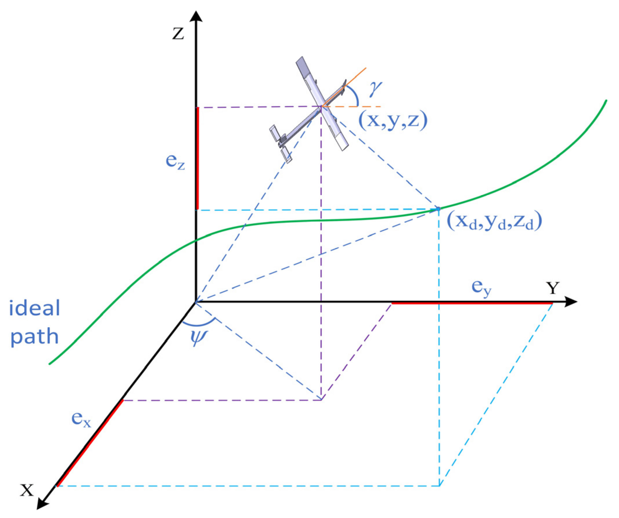
2.1. UAV Modeling

The positional relationship between a UAV and an ideal path in a three-dimensional space is shown in Figure 1.

In Figure 1, $(x,y,z)$ represents the position coordinates of the fixed-wing UAV at a certain point in space, and $(x_d,y_{\mathrm{d}},z_d)$ represents the position coordinates of the fixed-wing UAV on the ideal path in three-dimensional space. $(x_e,y_e,z_e)$ represents the error between the current position $(x,y,z)$ of the fixed-wing UAV and the corresponding position $(x_d,y_{\mathrm{d}},z_d)$ on the ideal path. The motion model of fixed-wing UAV in three-dimensional space is shown in Equation (1) [26]:

$$\left\{\begin{array}{l}\dot{x}=v\cos \psi \cos \gamma +d_x\\ \dot{y}=v\sin \psi \cos \gamma +d_y\\ \dot{z}=v\sin \gamma +d_z\end{array}\right.$$

(1)

where $\psi$ is the yaw angle, $\gamma$ is the flight path angle, and $v$ is the flight speed of the fixed-wing UAV. $d_x$, $d_y$, and $d_z$ are the unknown disturbances of each coordinate axis, respectively.

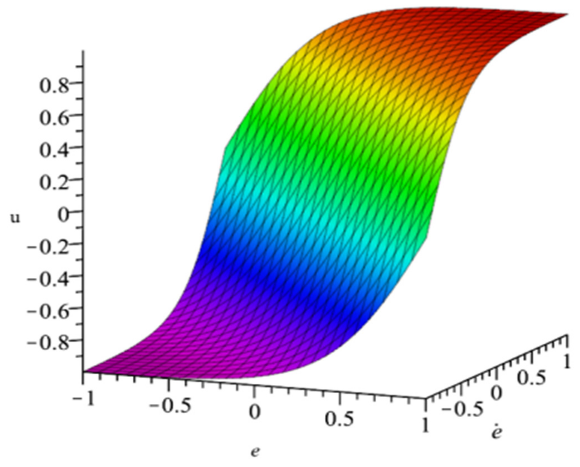
2.2. S-Plane Control

The S-Plane control model is shown in Equation (2):

$$u=\frac{2}{1+\exp [-(k_{11}e+k_{12}\dot{e})]}-1.0$$

(2)

where $e$ is the error of the input signal, $\dot{e}$ is the error change rate of the input signal, and $k_{11}$ and $k_{12}$ represent the adjustment coefficients of the input signal error and error change rate, respectively. A diagram of its three-dimensional surface is shown in Figure 2.

S-Plane control is similar in structure to proportional differential control. Therefore, in the adjustment of $k_{11}$ and $k_{12}$,we can refer to the adjustment mode of its parameters in proportional differential control. PD control is linear control, while S-Plane control is a kind of nonlinear control based on the fuzzy control table. Thus, it also has the advantages of strong robustness and anti-disturbance of fuzzy control.

In the path following a fixed-wing UAV, the mathematical model of the ideal path is $\zeta =f(t)$. It can be seen from Section 2 that $\mathrm{q} (x_{\mathrm{d}}, y_{\mathrm{d}},{ \mathrm{z}}_{\mathrm{d}})$ is a point on the ideal path. The current position of the fixed-wing UAV is $p (\mathrm{x}, \mathrm{y}, \mathrm{z})$. The purpose of path following is to make $\underset{t\to \infty }{\lim }\parallel p-q\parallel =0$ by designing a control law so as to achieve $x$ following $x_{\mathrm{d}}$,$y$ following $y_{\mathrm{d}}$,$z$ following $z_{\mathrm{d}}$. That is, the error of each coordinate axis in the three-dimensional space tends to be 0. The error equation is shown in Equation (3).

$$\left\{\begin{array}{l}{x}_{\mathrm{e}}=x-x_{\mathrm{d}}\\ y_{\mathrm{e}}=y-y_{\mathrm{d}}\\ z_{\mathrm{e}}=z-z_{\mathrm{d}}\end{array}\right.$$

(3)

The derivative of error can be obtained through the derivation of Equation (3) according to Equation (1). The derivative of error is shown in Equation (4).

$$\left\{\begin{array}{l}{\dot{x}}_{\mathrm{e}}=v\cos \psi \cos \gamma -{\dot{x}}_{\mathrm{d}}\\ {\dot{y}}_{\mathrm{e}}=v\sin \psi \cos \gamma -{\dot{y}}_{\mathrm{d}}\\ {\dot{z}}_{\mathrm{e}}=v\sin \gamma -{\dot{z}}_{\mathrm{d}}\end{array}\right.$$

(4)

In order to facilitate the design of late control law, we make a simple replacement, such as Equation (5).

$$\left\{\begin{array}{l}v\cos \psi \cos \gamma =U_1\\ v\sin \psi \cos \gamma =U_2\\ v\sin \gamma =U_3\end{array}\right.$$

(5)

3. Controller Design

3.1. GSISM S-Plane Controller and Stability Analysis

In order to design the three-dimensional path following the controller of the fixed-wing UAV, a theorem from the literature [27] is adopted.

Lemma 1: The trivial solution of the system

$$\dot{\eta }=-\alpha \tanh (k\eta )$$

(6)

is globally asymptotically stable for any selected constants $\alpha , k>0$, and for each $\eta (0)$, the state $\eta (t)$ converges exponentially to zero.

Proof: It is sufficient to prove that when $t\to \infty$, $\eta \to 0$. That is, when Equation (6) is asymptotically stable, Lyapunov is defined as $V={\eta }^2/2$.

Then,

$$\dot{V}=\eta \dot{\eta }=-\alpha \eta \tanh (k\eta )$$

(7)

since $x\tanh (x)=x\frac{e^x-e^{-x}}{e^x+e^{-x}}\ge 0$, $k\eta \tanh (k\eta )\ge 0$; thus, $\dot{V}\le 0$

if, and only if, $\eta =0$, $\dot{V}=0$

which completes the proof [28].

The above theorem is also used in reference [29] for the controller design of a wheeled mobile robot. The wheeled mobile robot is eventually able to track the ideal path with a certain accuracy. However, compared with fixed-wing UAVs, wheeled mobile robots have the problem of having fewer degrees of freedom. In this paper, based on the literature [27], a GSISM+RBF S-Plane control method is proposed to improve the path-following accuracy of a fixed-wing UAV. The specific control law is designed as follows:

Firstly, the $x$-axis direction is taken to design the control law, and the GSISM plane is taken as

$$s_1=x_e+c_1{\displaystyle {\int }_0^t{x}_{e}dt+a_1\tanh (p_1{x}_e),c_1,a_1,p_1\ge 0}$$

(8)

The time derivative of ${\dot{s}}_1$ is given by

$$\begin{array}{ll}{\dot{s}}_1& ={\dot{x}}_e+c_1{x}_e+a_1{p}_1{(1/\cosh (p_1{x}_e))}^2=\dot{x}-{\dot{x}}_d+c_1{x}_e+a_1{p}_1{(1/\cosh (p_1{x}_e))}^2\hfill \\ & =u_1+d_x-{\dot{x}}_d+c_1{x}_e+a_1{p}_1{(1/\cosh (p_1{x}_e))}^2\hfill \end{array}$$

(9)

The control law in the $x$-axis direction can be designed as

$$u_1={\dot{x}}_d-c_1{x}_e-a_1{p}_1{(1/\cosh (p_1{x}_e))}^2-d_x-k_1{s}_1$$

(10)

Because $d_x$ is unknown, $d_x$ is estimated using an RBF neural network. The formula of the RBF neural network is

$$h(x)=\exp (\frac{{‖x-c_j‖}^2}{2b_j^2})$$

(11)

Design $d_x=d_1^{*}{}^{T}h(x)+{\epsilon }_x$

where $x$ is the input of the neural network, $j$ is the number of nodes in the hidden layer of the network, $h(x)$ is the output part of the Gaussian function, $d_1^{*}$ is the ideal weight, and ${\epsilon }_x$ is the approximation error.

In the $x$ direction, the actual output of the RBF neural network is

$${\widehat{d}}_x={\widehat{d}}_1{}^{T}h(x)$$

(12)

Then, Equation (10) can be rewritten as

$$u_1={\dot{x}}_d-c_1{x}_e-a_1{p}_1{(1/\cosh (p_1{x}_e))}^2-{\widehat{d}}_x-k_1{s}_1$$

(13)

Substitute Equation (13) into Equation (9) to obtain

$$\begin{array}{ll}{\dot{s}}_1& =u_1+d_x-{\dot{x}}_d+c_1{x}_e+a_1{p}_1{(1/\cosh (p_1{x}_e))}^2\hfill \\ & =({\dot{x}}_d-c_1{x}_e-a_1{p}_1{(1/\cosh (p_1{x}_e))}^2-{\widehat{d}}_x-k_1{s}_1)\hfill \\ & +d_x^{*}-{\dot{x}}_d+c_1{x}_e+a_1{p}_1{(1/\cosh (p_1{x}_e))}^2\hfill \\ & =-{\widehat{d}}_x+d_x-k_1{s}_1=-{\tilde{d}}_x-k_1{s}_1\hfill \end{array}$$

(14)

$${\tilde{d}}_x=d_x-{\widehat{d}}_x=d_1^{*}{}^{T}h(x)+{\epsilon }_x-{\widehat{d}}_1{}^{T}h(x)={\tilde{d}}_x{}^{T}h(x)+{\epsilon }_x$$

(15)

Define the Lyapunov function as

$$L_1=\frac{1}{2}{s}_1{}^2+\frac{1}{2}{\gamma }_1{\tilde{d}}_x{}^T{\tilde{d}}_x$$

(16)

The time derivative of $L_1$ is given by

$$\begin{array}{ll}{L}_1& =s_1{\dot{s}}_1+{\gamma }_1{\tilde{d}}_x{}^T{\dot{\tilde{d}}}_x\hfill \\ & =s_1(-{\tilde{d}}_x-k_1{s}_1)-{\gamma }_1{\tilde{d}}_x{}^T{\dot{\widehat{d}}}_x\hfill \\ & {=\mathrm{s}}_1(-{\tilde{d}}_x{}^{T}h(x)-{\epsilon }_x-k_1{s}_1)-{\gamma }_1{\tilde{d}}_x{}^T{\dot{\widehat{d}}}_x\hfill \\ & =-{ \mathrm{d} ˜}_x{}^T(s_{1}h(x)+{\gamma }_1{\dot{\widehat{d}}}_x)-k_1{s}_1{}^2-s_1{\epsilon }_x\hfill \end{array}$$

(17)

The adaptive rate of the designed $x$ axis is

$${\dot{\widehat{d}}}_x=-\frac{1}{{\gamma }_1}{s}_{1}h(x)$$

(18)

Then, ${\dot{L}}_1=s_1(-k_1{s}_1-{\epsilon }_x)=-k_1{s}_1{}^2-{\epsilon }_x{s}_1$; when ${\epsilon }_x$ is small enough, that is ${\epsilon }_x\to 0$, ${\dot{L}}_1\le 0$.

Similarly, the GSISM function in the $y$ direction can be designed as

$$s_2=y_e+c_2{\displaystyle {\int }_0^t{y}_{e}dt+a_2\tanh (p_2{y}_e),c_2,a_2,p_2\ge 0}$$

(19)

The control law in the $y$-axis direction can be designed as

$$u_2={\dot{y}}_d-c_2{y}_e-a_2{p}_2{(1/\cosh (p_2{y}_e))}^2-d_y-k_2{s}_2$$

(20)

Finally, the GSISM function in the $z$ direction can be designed as

$$s_3=z_e+c_3{\displaystyle {\int }_0^t{z}_{e}dt+a_3\tanh (p_3{z}_e),c_3,a_3,p_3\ge 0}$$

(21)

The control law in the $z$-axis direction can be designed as

$$u_3={\dot{z}}_d-c_3{z}_e-a_3{p}_3{(1/\cosh (p_3{z}_e))}^2-d_z-k_3{s}_3$$

(22)

When ${\dot{L}}_i\equiv 0(i=1,2,3)$, $s_i\equiv 0(i=1,2,3)$, according to the invariance principle of $LaSalle$, the closed-loop system is asymptotically stable.

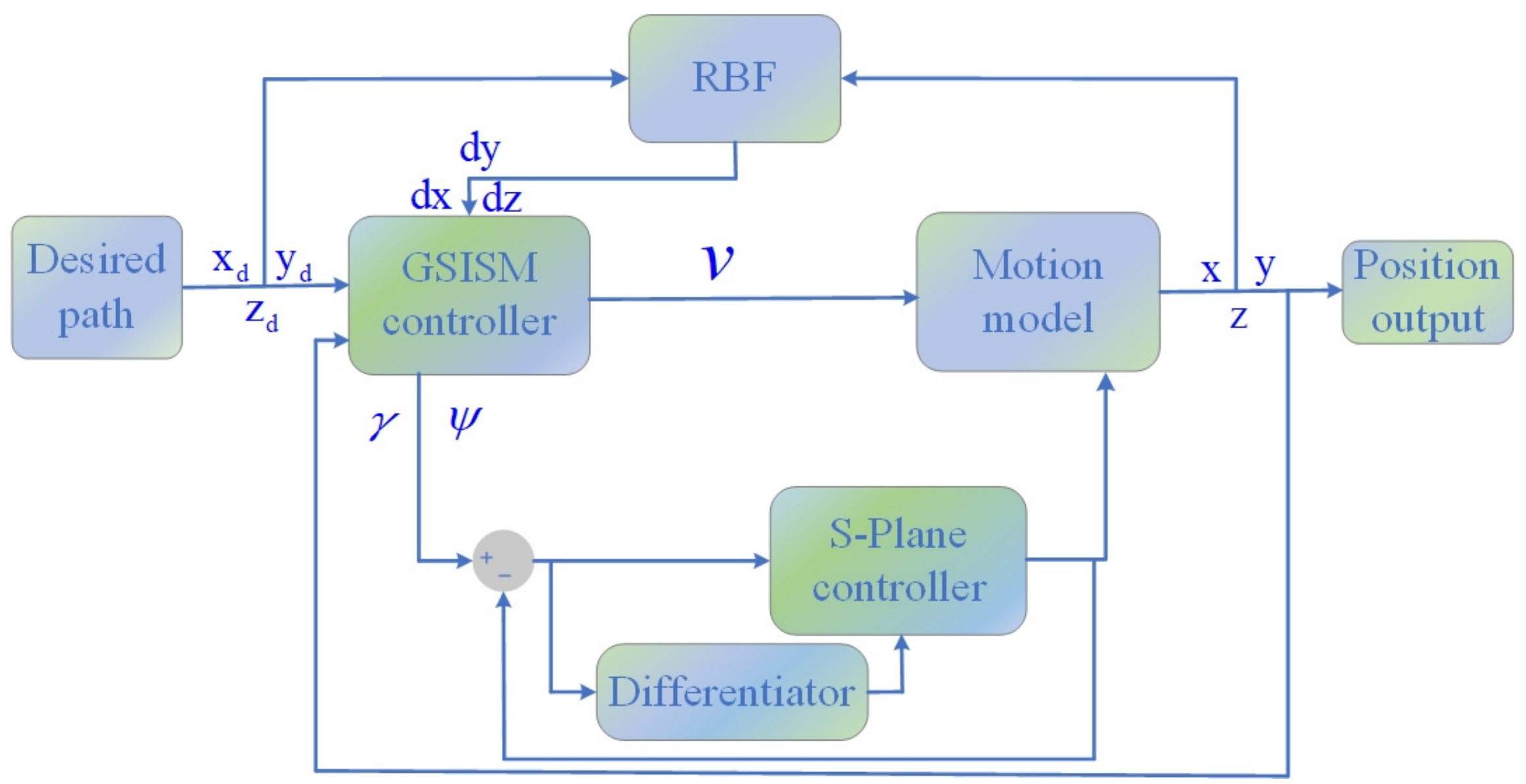
3.2. Controller Structure

The structure of the fixed-wing UAV path-following controller proposed in this paper is shown in Figure 3.

GSISM+RBF S-Plane controller adopts the double-loop structure of inner and outer loop control. The running process of the GSISM+RBF S-Plane controller is as follows. Firstly, an ideal flight path is obtained through the track generator. Then, the ideal path is expressed in the form of a parametric equation and transmitted to the GSISM controller. Flight speed $v$, flight path angle $\gamma$, and yaw angle $\psi$ are obtained under the action of the GSISM controller, where the flight speed $v$ is transmitted to the motion model through the outer loop control. The flight path angle $\gamma$ and yaw angle $\psi$ are transmitted to the motion model after passing through the S-Plane control in the inner loop. The actual UAV flight path coordinate is obtained after the action of the motion model. A part of the signal is output, and another part is fed back to the input signal to participate in the calculation of the next step. By repeating this process, the fixed-wing UAV can follow the ideal path. When the flight path angle $\gamma$ and yaw angle $\psi$ are transmitted to the inner loop control, the error of the flight path angle $\gamma$ and yaw angle $\psi$ is obtained under the action of the feedback signal. Then, the error change rate is obtained under the action of the differentiator, and the obtained error and error change rate are transmitted to the S-Plane controller. Part of the signal is output to the kinematic model after the action of the S-Plane controller; another part of the signal is fed back to the input signal of the inner loop control to participate in the calculation of the next step in the inner loop control. In addition, the RBF neural network takes the error of the input expected position and output actual position as the input signal and its output signal is input to the GSISM controller as the estimated value of unknown disturbance. In this way, the following of the intermediate command signal can be realized. The intermediate command signal can be obtained by Equation (5). The yaw angle $\psi$ of path following is

$$\psi =\arctan (\frac{U_2}{U_1})$$

(23)

The flight path angle $\gamma$ of the path to be followed can be obtained according to Equations (5) and (23).

$$\gamma =\arctan (\frac{U_3}{U_2}\sin \psi )$$

(24)

The velocity $v$ of the path to be followed is obtained according to Equations (5), (23), and (24).

$$v=\frac{U_3}{\sin \gamma }$$

(25)

The input signal in S-Plane control is the error and error change rate. Integral explosion in the solution of the error change rate occurs easily. Therefore, the derivation process of the intermediate instruction signal is realized using the second-order differential method [28]. The second-order differentiator is shown in Equation (26):

$$\left\{\begin{array}{l}{\dot{x}}_1=x_2\\ {\dot{x}}_2=-2R^2(x_1-n(t))-R{x}_2\\ y=x_2\end{array}\right.$$

(26)

where $n(t)$ is the input signal, $x_1$ is the following of the signal, and $x_2$ is the estimation for the first-order derivative of the signal. The differentiator is an integral chain operation, which can suppress the noise in signal derivation.

3.3. GSISM+RBF S-Plane Control Algorithm

The path-following control algorithm based on GSISM+RBF S-Plane model for the fixed-wing UAV is shown as Algorithm 1.

Algorithm 1: GSISM+RBF S-Plane Controller

Outer loop input: expected path point $\mathrm{q} (x_{\mathrm{d}}, y_{\mathrm{d}},{ \mathrm{z}}_{\mathrm{d}})$. Current location point $p (\mathrm{x}, \mathrm{y}, \mathrm{z})$. GSISM+RBF S-Plane control gain. $dx, dy, dz$. Inner loop input: intermediate command signal $\psi$,$\gamma$, S-Plane gain $k_{11}$,$k_{12}$,$k_{21}$,$k_{22}$. 1: calculating the error and error change rate through Equations (3) and (4). 2: $(s_1,s_2,s_3)\leftarrow (x_e,y_e,z_e)$ 3: calculate $u_1,u_2,u_3$ through Equations (10), (20), and (22) 4: calculate $\psi ,\gamma ,v$ through Equations (23)–(25) 5: calculating $\dot{\psi }$ and $\dot{\gamma }$ through Equation (26). 6: $(e_{\psi },e_{\gamma })\leftarrow (\psi -{\psi }^{\prime },\gamma -{\gamma }^{\prime })$ 7: ${\psi }^{\prime }\leftarrow 2/(1+\exp [-(k_{11}{e}_{\psi }+k_{12}{\dot{e}}_{\psi })])-1.0$ 8: ${\gamma }^{\prime }\leftarrow 2/(1+\exp [-(k_{21}{e}_{\gamma }+k_{22}{\dot{e}}_{\gamma })])-1.0$ 9: inner loop return: ${\psi }^{\prime }$,${\gamma }^{\prime }$ 10: $(x,y,z)\leftarrow (v\cos {\psi }^{\prime }\cos {\gamma }^{\prime },v\sin {\psi }^{\prime }\cos {\gamma }^{\prime },v\sin {\gamma }^{\prime })$ 11: outer loop return:$x$,$y$,$z$

4. Simulation and Results Analysis

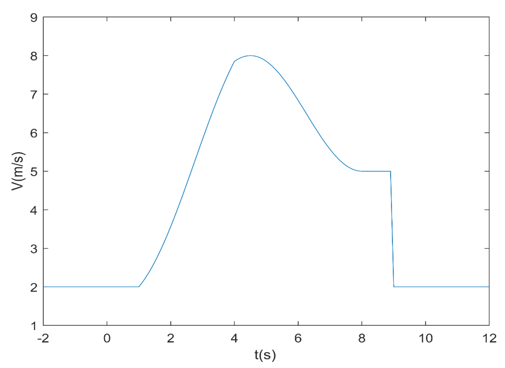
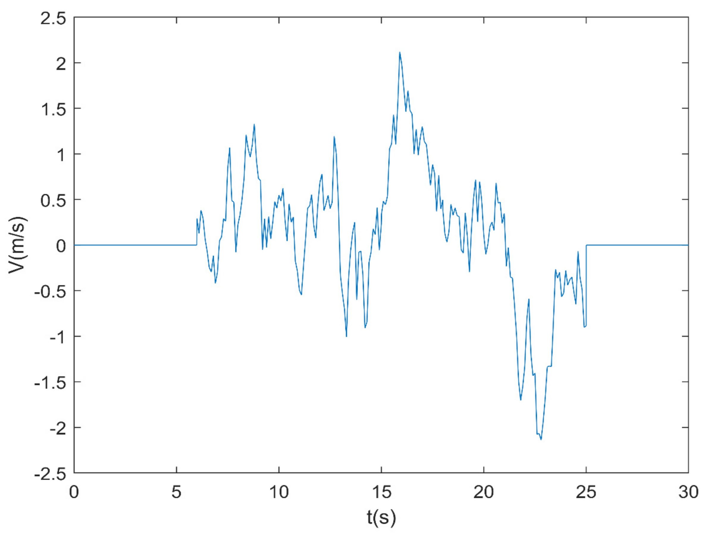
4.1. Wind Disturbance Modeling

In the design of a small fixed-wing UAV controller, the factor of wind has a great influence on the performance of the designed controller. In the field of wind power generation, in-depth research has been carried out on the composition and performance of wind. Therefore, we can refer to these research results to study the impact of external wind disturbance on small fixed-wing UAVs. Wei et al. hypothesize that the wind occurring in nature is composed of basic wind, gust wind, gradual wind, and random wind and that the random combinations of these four types of wind represent most wind types occurring in nature [25]. However, the wind speed used in wind power generation is generally low, which is not fully applicable to wind disturbance modeling in the control process of a fixed-wing UAV. So, based on relevant research results, this paper further studies a wind disturbance model affecting the control of a fixed-wing UAV; adjustment factors, including gust, gradual wind, and random wind, are added to adjust the wind speed according to different needs.

(1)

Basic Wind

Basic wind describes an average change in the external wind. It is also the best wind speed for UAV flights. In most cases, the wind occurring in nature can be described as basic wind. We treat it as a constant when we simulate it.

$$V_c=k, \mathrm{k} \mathrm{is} \mathrm{a} \mathrm{constant}$$

(27)

(2)

Gust Wind

Gust is a wind whose wind direction remains unchanged and whose wind speed increases suddenly for a short time. It reflects a sudden change in the wind. The model of gust wind can be expressed as follows:

$$V_g=\left\{\begin{array}{l}0,{ \mathrm{t}<\mathrm{t}}_1\\ k_g\cdot \frac{V_{g\max }}{2}\left[1-\cos (2\pi (\frac{t-t_1}{t_g}))\right]\\ 0,{ \mathrm{t}>\mathrm{t}}_1+t_g\end{array}\right.,{ \mathrm{t}}_1\le t\le t_1+t_g$$

(28)

where $V_g$ is the wind speed of the gust, $V_{g\max }$ is the highest wind speed of the gust, $t_1$ is the start time of the gust, $t_g$ is the duration of the gust, and $k_g$ is the gust wind speed adjustment factor.

(3)

Gradual Wind

Gradual wind reflects a gradual nature in the wind, and its model can be expressed as follows:

$$V_w=\left\{\begin{array}{l}0, \mathrm{others}\\ k_w\cdot V_{w\max }\frac{t-t_2}{t_3-t_2},{ \mathrm{t}}_2\le t\le t_3\\ k_w\cdot V_{w\max },{ \mathrm{t}}_3<t\le t_3+T\end{array}\right.$$

(29)

where $V_w$ is the wind speed of the gradual wind, $V_{w\max }$ is the maximum wind speed of the gradual wind, $t_2$ is the start time of the gradual wind, $t_3$ is the end time of the gradual wind, $T$ is the holding time of the gradual wind, and $k_w$ is the wind speed adjustment factor of the gradual wind.

(4)

Random Wind

Random wind reflects arbitrariness, uncertainty, and randomness of wind, and its model is shown as follows:

$$V_n=k_n\cdot V_{n\max }{R}_{am}(-1,1)\cos (\omega +\phi )$$

(30)

where $k_n$ is the adjustment factor of random wind speed, $V_n$ is the random wind speed, $V_{n\max }$ is the maximum random wind speed, $R_{am}(-1,1)$ is a random number between −1 and 1, and $\omega$ is the average distance of the wind speed fluctuation. The general value is $0.5\pi \sim 2\pi$; $\phi$ is a random quantity uniformly distributed on $0\sim 2\pi$. After modeling the above four kinds of wind, we can represent the influence of real external wind on a small fixed-wing UAV flight in any combination. This is of great significance for improving the control performance of small fixed-wing UAVs. The following are the simulation results obtained by randomly selecting a combination of several winds.

Bring $V_c=2\mathrm{m}/\mathrm{s}$, $k_g=0.5\mathrm{m}/\mathrm{s}$, $V_{g\max }=6\mathrm{m}/\mathrm{s}$, $t_1=1$, $t_g=7$, $k_w=0.5$, $V_{w\max }=6$ into the gust and gradual wind formula above. The results for a combination of basic wind, gradual wind, and gust can be obtained via the MATLAB simulation, as shown in Figure 4.

The simulation of the random wind function is complex, so we approximately estimate the arbitrary wind model of nature through the random number module, transfer Fcn module, and gain module in Simulink. Bring $k_g=0.125\mathrm{m}/\mathrm{s}$, $V_{g\max }=8\mathrm{m}/\mathrm{s}$, $t_1=15\mathrm{m}/\mathrm{s}$, $t_g=3\mathrm{m}/\mathrm{s}$ into the random wind and gust formula above. The simulation of a specific random wind and gust combination model is shown in Figure 5.

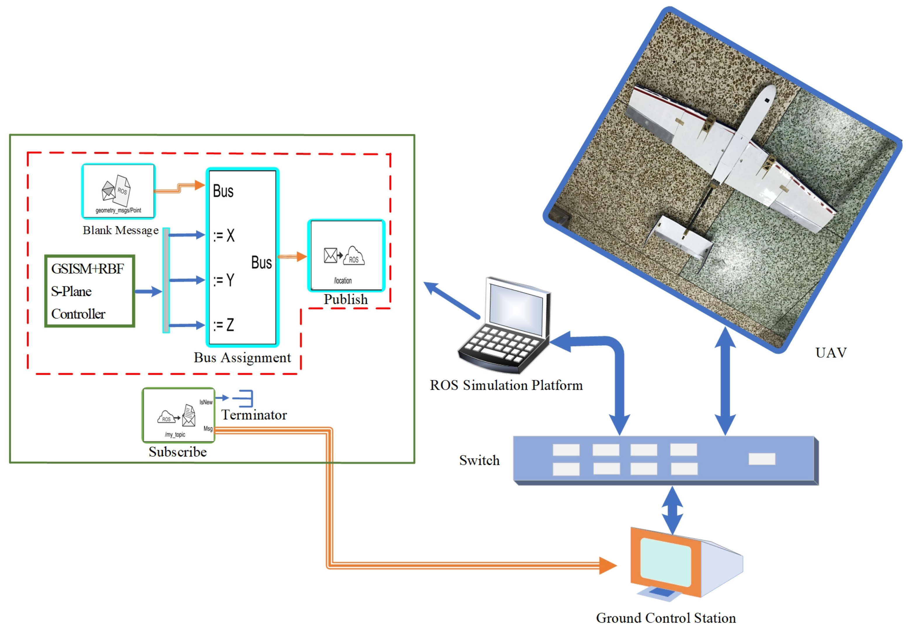
4.2. Semi-Physical Simulation System

The hardware in the loop simulation system used in this paper is shown in Figure 6. It consists of four parts, namely, a ground control station, a switch, a UAV, and a ROS simulation platform. During operation, communication between the ROS simulation platform, UAV, and ground control station is achieved through the switch; the ROS simulation platform sends the simulation results to the ground control station through the switch-and-subscribe method. Then, the ground control station sends the control command to the UAV’s airborne computer through the switch to control the flight of the UAV. The simulation principle of the ROS simulation platform is as follows. In Figure 6, the inner part of the red dotted box is the publisher creation process, and the rest is the subscriber creation process. During the creation of the publisher, when the blank message module outputs a ROS message (bus signal) to the bus assignment module, the GSISM+RBF S-Plane controller module designed in this paper generates a UAV path following specific points, which are relayed via a ROS message under the action of the bus assignment module. Then, the bus assignment module passes the ROS message containing the UAV path points onto the publish module. After receiving the bus signal, the publish module sends it to the topic of “/location.” During the creation process of the subscriber, the subscribe module subscribes to the messages sent to the “/my_topic” by the publisher and extracts the coordinates of the UAV path points from the message, and then transfers these to the ground control station. The UAV model includes the shape and size design of the UAV, mainly to maintain its similarity to the actual UAV. It also includes a dynamic model based on Newtonian mechanics, a sensor model considering sensors such as cameras and radars, and a controller model based on control theory and UAV control characteristics.

4.3. Simulation Test and Results Analysis

In order to verify the following accuracy and anti-disturbance performance of the GSISM+RBF S-Plane controller designed in this paper, the GSSM controller in reference [29] and the GSISM S-Plane controller are used for a comparative experiment. In addition, the control effect under different flight paths following a spatial straight line, a spiral line, and a special space curve is verified. The coefficient of two S-Plane controllers is shown in

Table 1. The coefficient of two S-Plane controllers.

	${\mathit{k}}_{11}^{\prime }$	${\mathit{k}}_{12}^{\prime }$	${\mathit{k}}_{21}^{\prime }$	${\mathit{k}}_{22}^{\prime }$
two S-Plane controllers	4	0.01	10	0.1

.

Where the unknown disturbances in Equation (1) are:

$$\left\{\begin{array}{l}dx=5\sin (0.5t)\\ dy=5\cos (0.5t)\\ dz=5\sin (0.5t)\end{array}\right.$$

(31)

The coefficient of the RBF function is shown in

Table 2. The coefficient of the RBF function.

	${\mathit{c}}_{\mathit{i}\mathit{j}}$	${\mathit{b}}_{\mathit{j}}$	${\mathit{\gamma }}_1$	${\mathit{\gamma }}_2$	${\mathit{\gamma }}_3$
RBF function	$0.1\left(\begin{array}{c}-0.5\\ -0.5\end{array}\begin{array}{c}-0.25\\ -0.25\end{array}\begin{array}{c}0\\ 0\end{array}\begin{array}{c}0.25\\ 0.25\end{array}\begin{array}{c}0.5\\ 0.5\end{array}\right)$	15	50	50	50

.

The parameters of the GSISM function in adaptive estimation are $a_{1i}=c_{1i}=p_{1i}=0.015 (i=1,2,3)$. The GSISM+RBF S-Plane control coefficients for the UAV when tracking the spatial straight line, spiral line, and special spatial curve are shown in

Table 3. The GSISM+RBF S-Plane control coefficients for the UAV when tracking the spatial straight line, spiral line, and special spatial curve.

	k1	k2	k3	c1	c2	c3	a1	p1	a2	p2	a3	p3
spatial straight line	0.5	0.0165	0.09	3	20	20	40	0.2	5	1.1	2	0.2
spiral line	7	30	30	0.20	0.3	0.3	2	0.2	13.4	10	2	0.2
special spatial curve	4	5	9	8	10	15	2	0.2	0.5	1.1	0.2	0.2

.

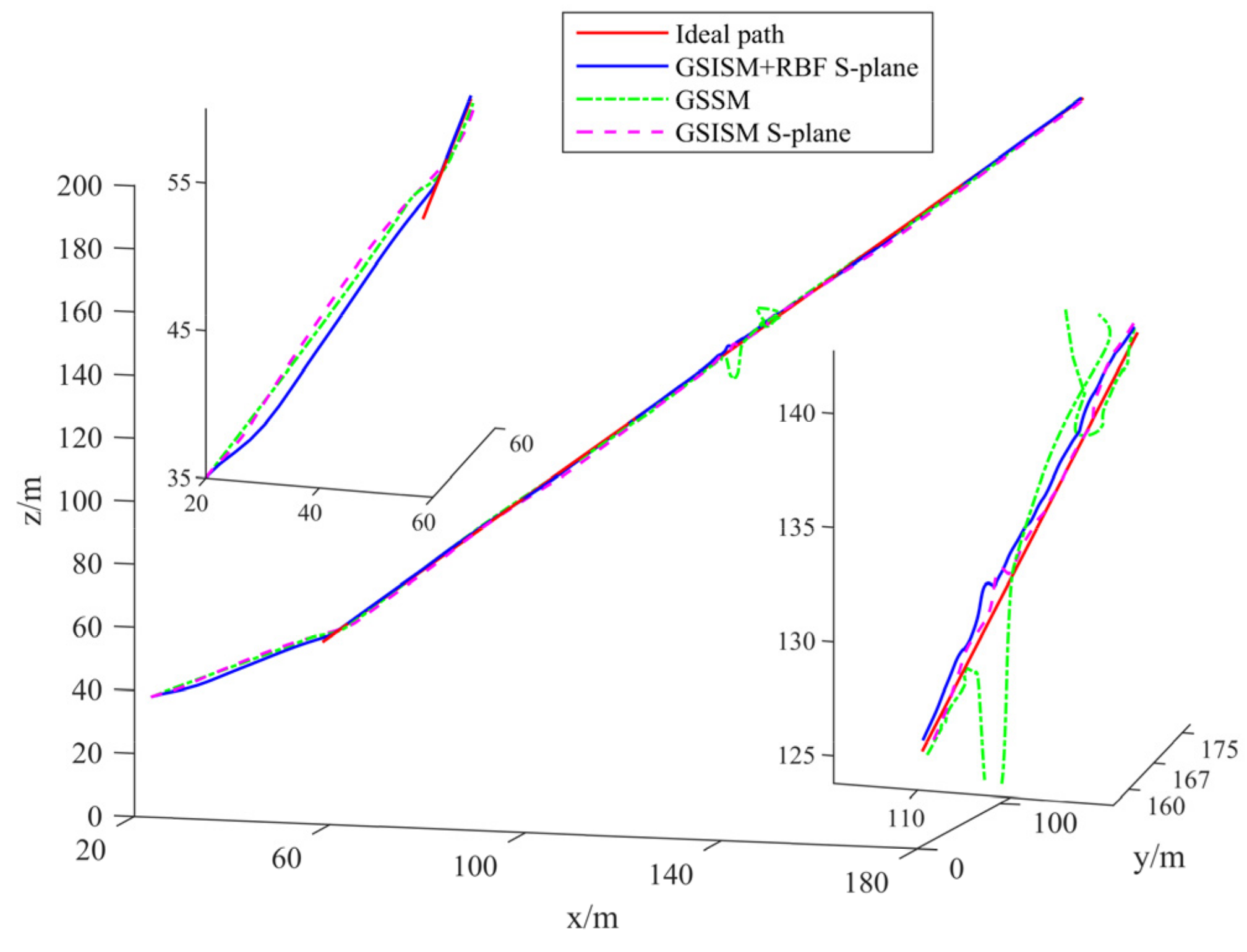
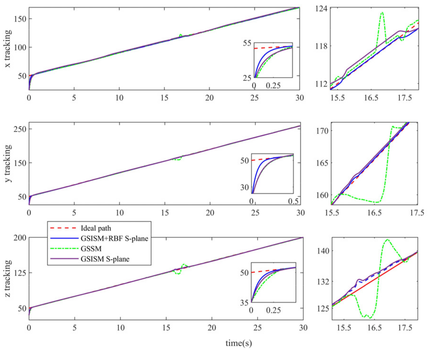
4.3.1. Spatial Straight Line Path-Following Simulation

The parameter expression when the ideal path followed by the fixed-wing UAV is a spatial straight line is shown by Equation (32):

$$\zeta :\left\{\begin{array}{l}{x}_d=50+4t\\ y_d=50+7t\\ z_d=50+5t\end{array}\right.$$

(32)

The initial position of a fixed-wing UAV during takeoff when following a spatial straight line is calculated in $[20,20,35]$. Under the action of control laws, the fixed-wing UAV completes the flight process along the spatial straight line. A diagram of the spatial straight line followed by the fixed-wing UAV in the simulation is shown in Figure 7. The error diagram of each coordinate is shown in Figure 8. As can be seen from Figure 8, when the fixed-wing UAV flies in a spatial straight line, the GSISM+RBF S-Plane controller can cut into the ideal path smoothly and quickly compared with the GSSM controller and GSISM S-Plane control. Figure 9 shows the error diagram of each coordinate axis of the spatial straight line. It can be seen from Figure 9 that in the whole flight process, especially when a disturbance is added in at around 10–20 s, the error between GSISM+RBF S-Plane control and the desired path is basically 0, which is smaller than that achieved with GSSM control and GSISM S-Plane control. Therefore, the GSISM+RBF S-Plane controller has the advantages of high following accuracy and strong anti-disturbance ability.

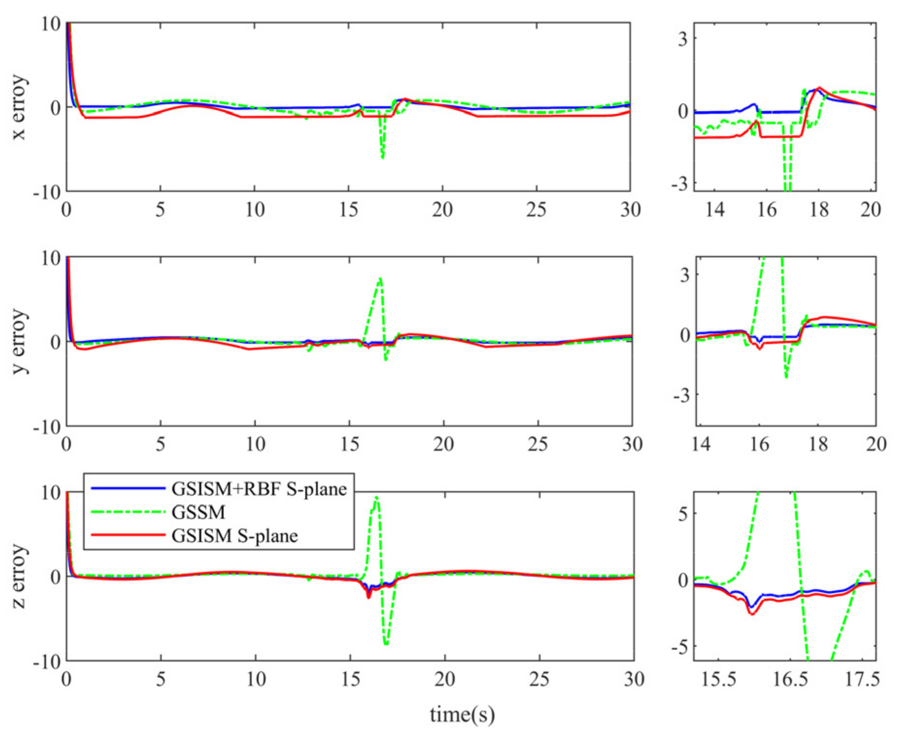
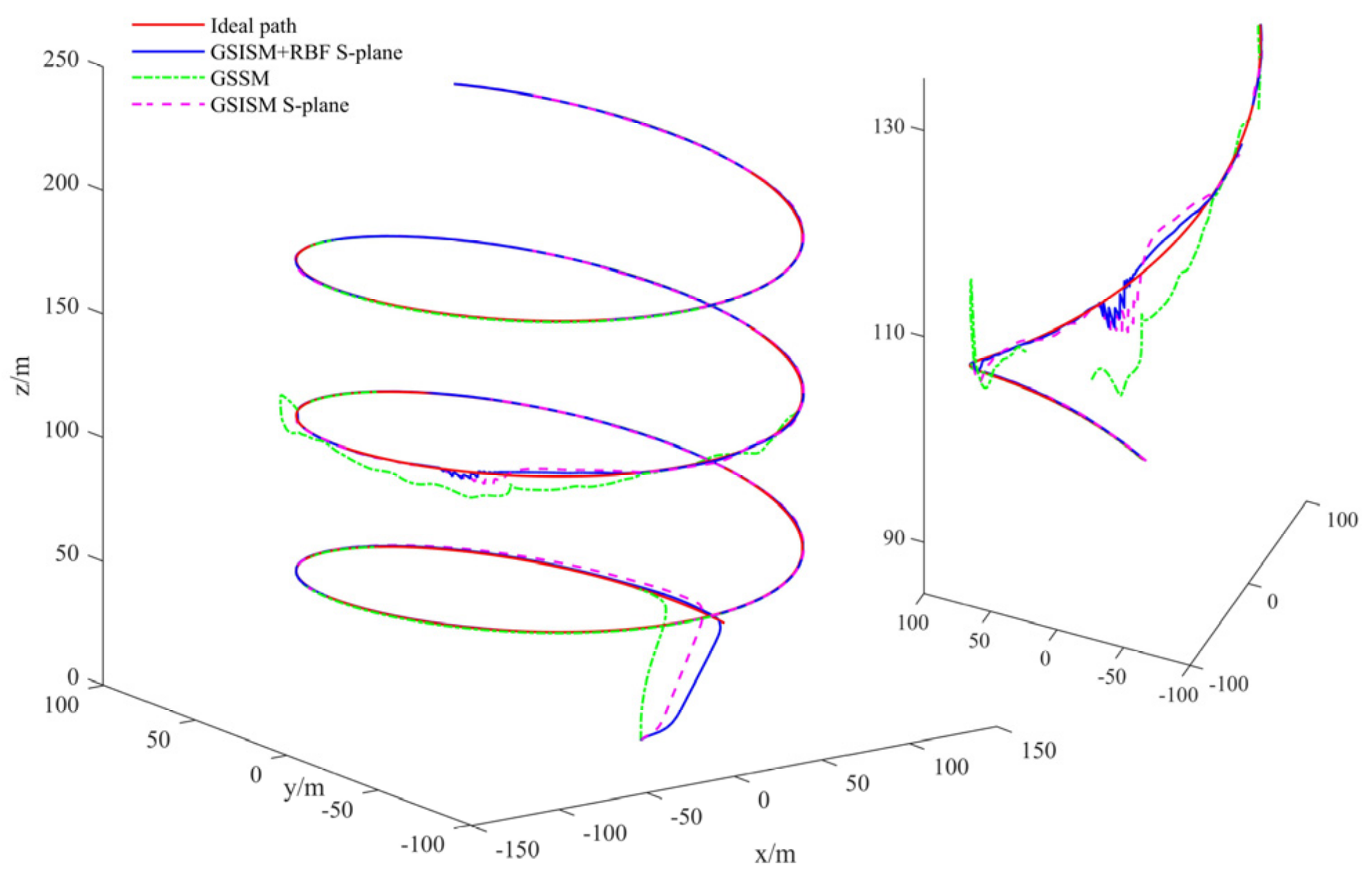
4.3.2. Spiral Line Path following Simulation

When the ideal flight path of the fixed-wing UAV is a circle, in order to better reflect the following performance of the designed controller in practice, the simulation is carried out using a spiral instead of a circle. The parametric equation of the spiral line is shown in Equation (33).

$$\zeta :\left\{\begin{array}{l}{x}_d=100\cos (t/2)\\ y_d=100\sin (t/2)\\ z_d=20+5t\end{array}\right.$$

(33)

When flying along the spiral line, the initial position of UAV takeoff is $[0,0,0]$ in the GSISM+RBF S-Plane controller. The simulation results for the fixed-wing UAV following the spiral line flight path are shown in Figure 10.

It can be seen from Figure 10 that GSISM+RBF S-Plane control, GSSM control, and GSISM S-Plane control had good control performances and could track the ideal path with high accuracy. However, compared with GSSM control and GSISM S-Plane control, GSISM+RBF S-Plane control could cut into the ideal path with a certain radian. GSSM control and GSISM S-Plane control cannot track with high accuracy in the initial stage and only cut into the ideal path after a few seconds. Figure 11 is the path-following diagram of each coordinate axis when the UAV follows the spiral line. Figure 12 shows the error value between the ideal path and the actual flight path of each coordinate axis when the UAV follows the spiral line. In the whole flight segment of Figure 12, the error of GSISM+RBF S-Plane control is around 0. It can be seen that the path-following accuracy is particularly high. In addition, we added the wind disturbance designed in Section 4 at around 15–25 s into the spiral line path-following simulation. It can be seen from Figure 11 and Figure 12 that when there is a gust disturbance at 17–23 s, the fluctuation of the UAV flying along the ideal path is greater. Compared with GSSM control and GSISM S-Plane control, GSISM+RBF S-Plane control leads to less fluctuation in gust disturbance. It can be seen that its performance against external wind disturbance is superior.

Figure 13 and Figure 14 present input and output diagrams of the flight path angle and yaw angle in S-Plane control. S-Plane control has good anti-disturbance performance. It can be seen from Figure 13 and Figure 14 that the output value of the command signal is significantly different from the input value after being controlled by the S-Plane, regardless of the flight path angle or yaw angle. The corresponding value is large before entering the S-Plane controller, but after the action of the S-Plane controller, it is basically normalized to $[-1,1]$. Although the intermediate command signal changes to a certain extent when passing through the S-Plane control, the path-following accuracy of the fixed-wing UAV does not change; this also shows that the GSISM+RBF S-Plane controller designed in this paper has good control performance.

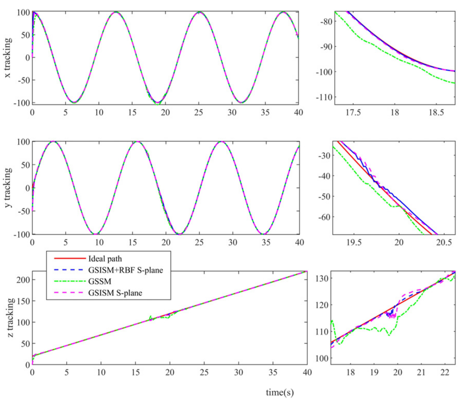
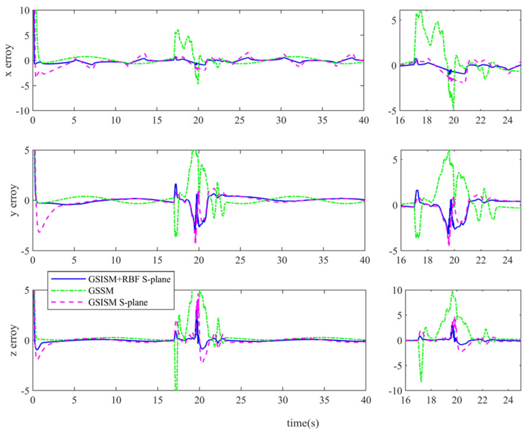
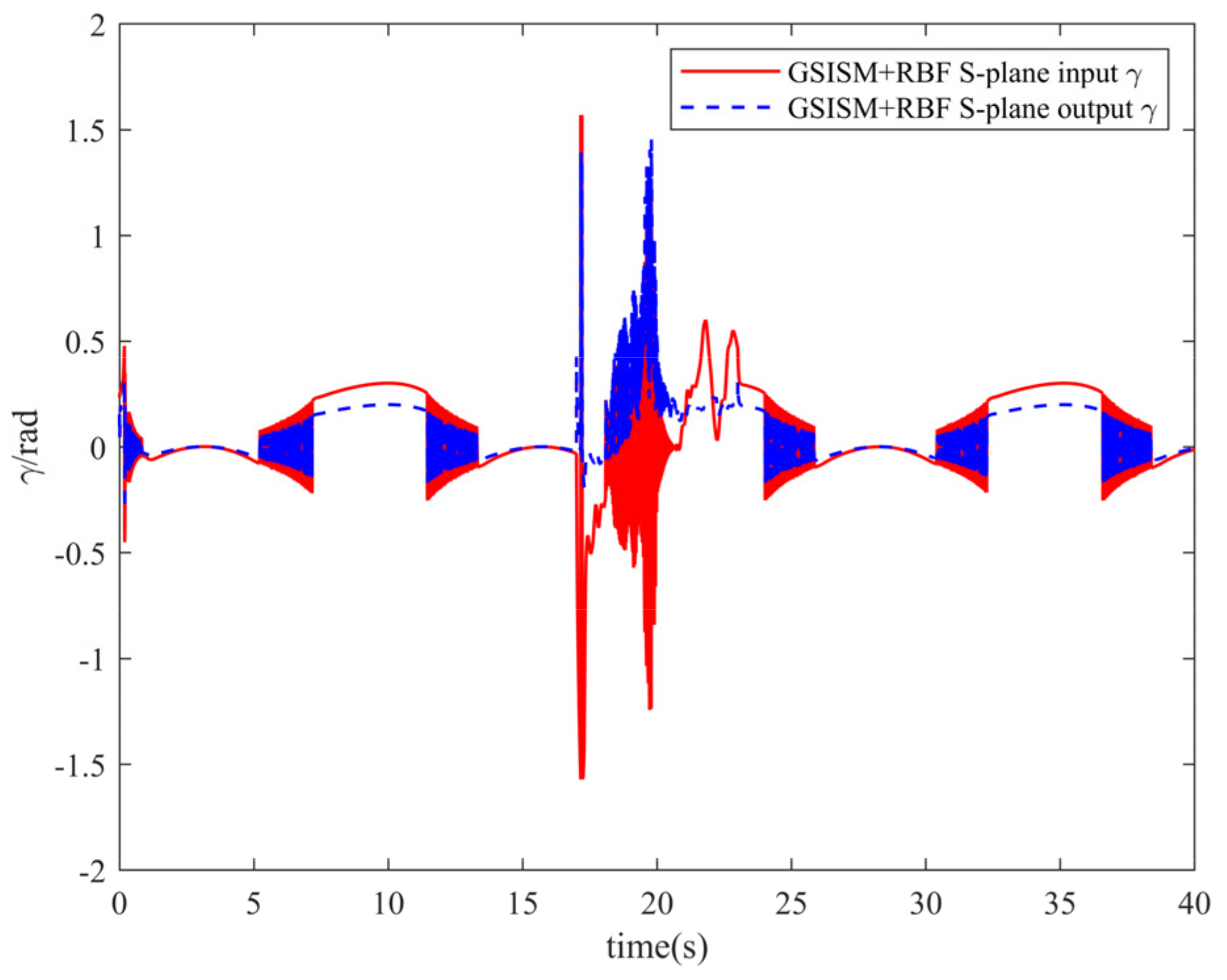
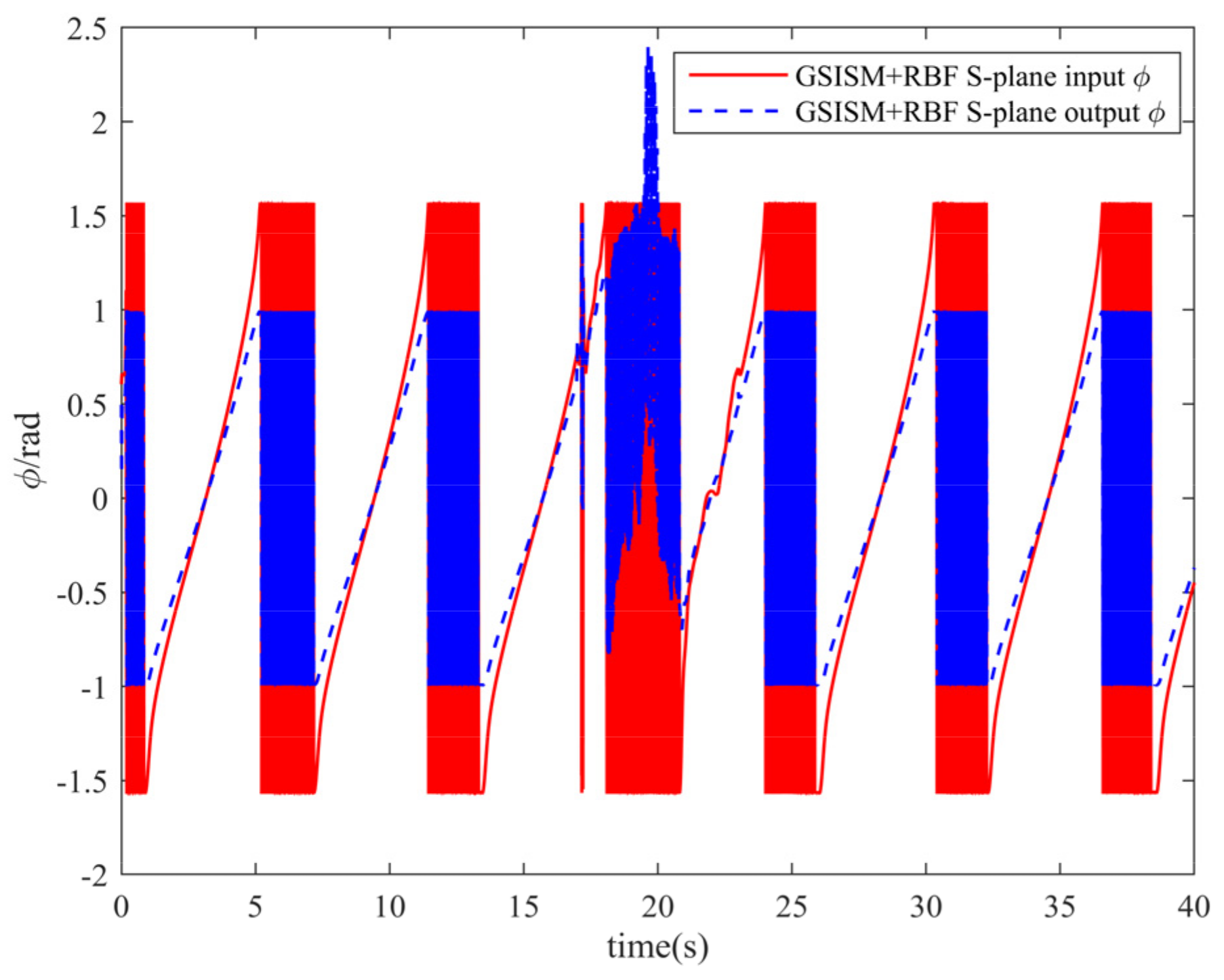
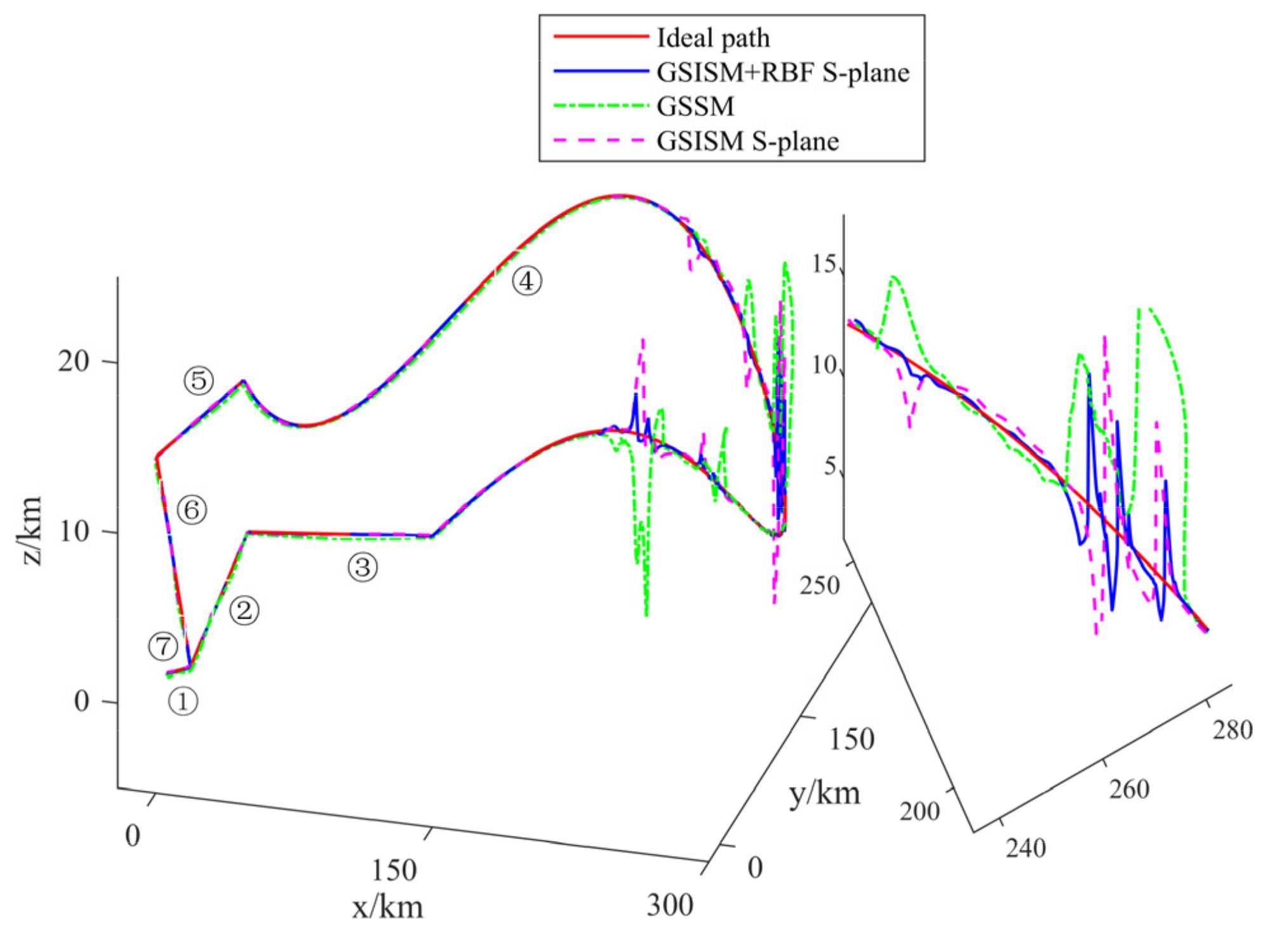
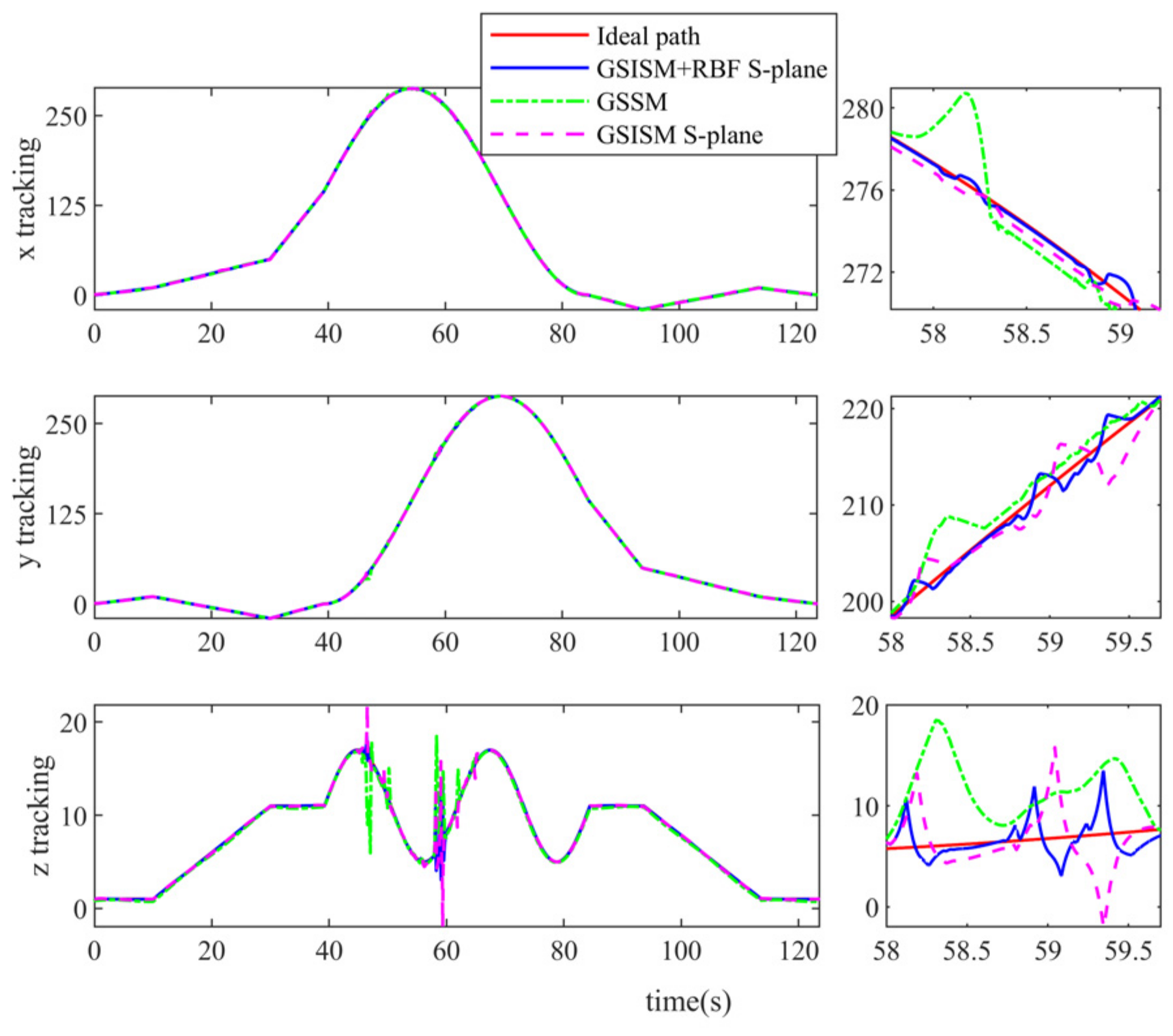
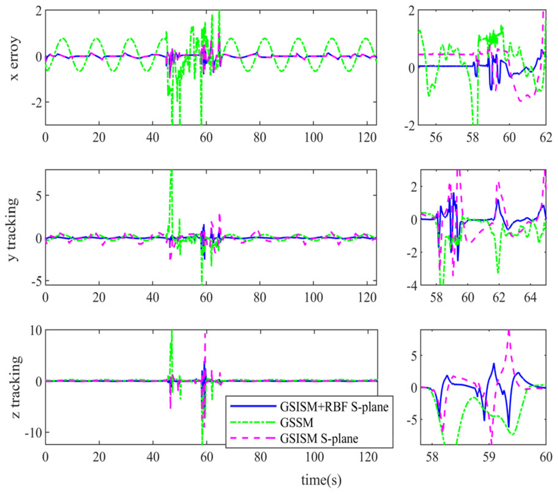
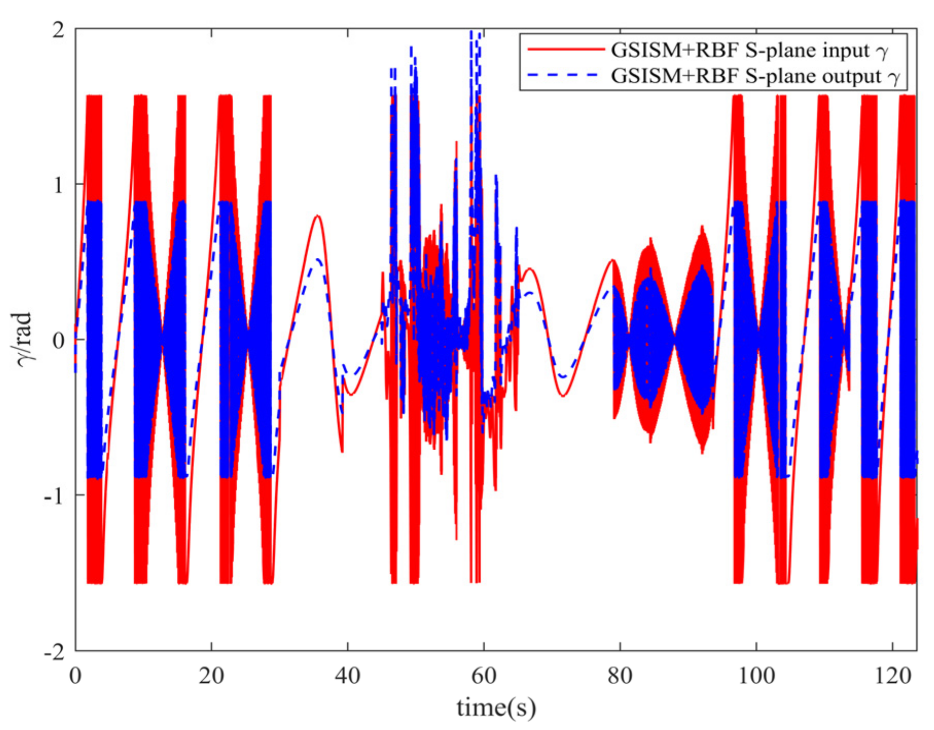
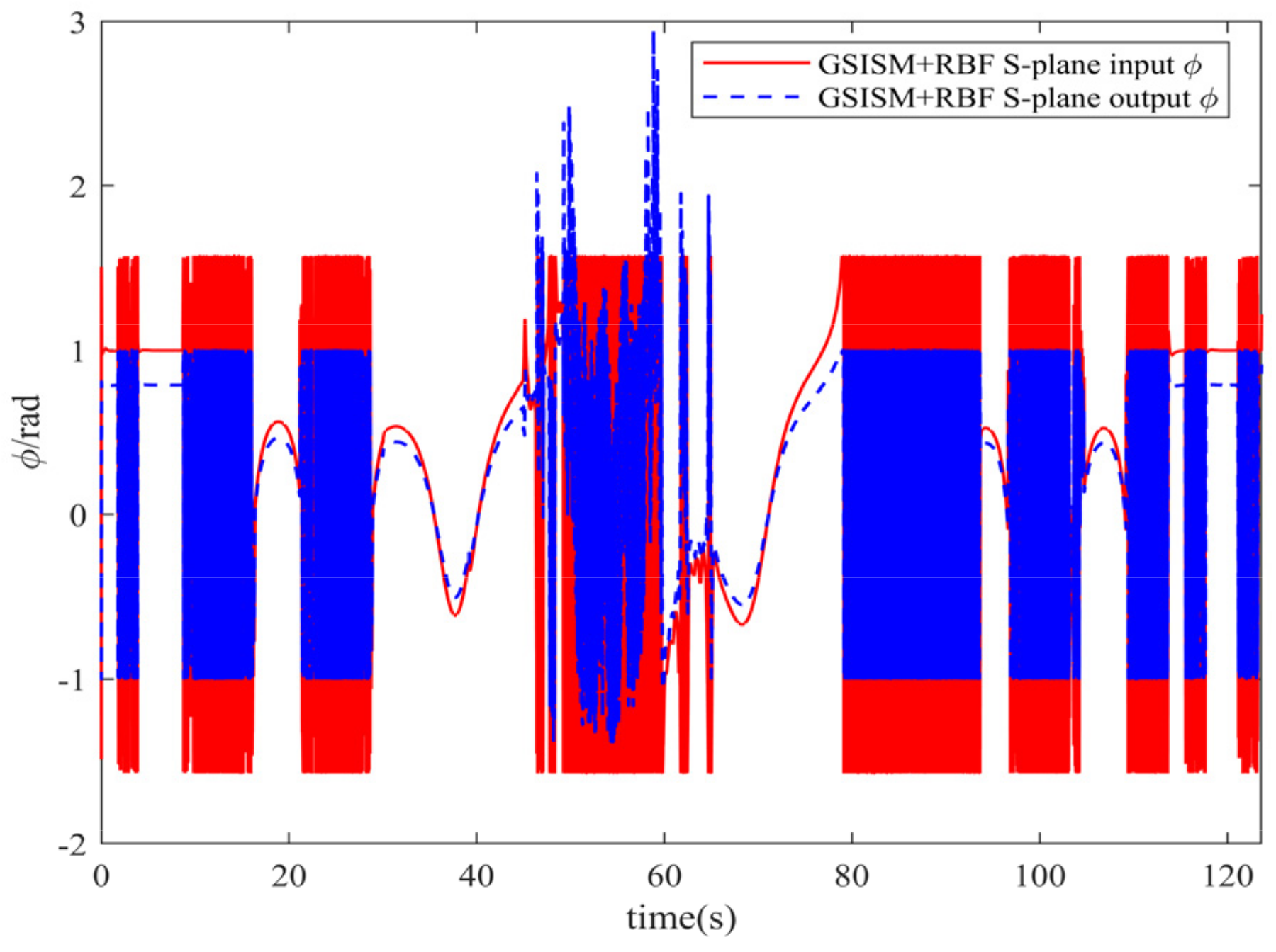
4.3.3. Following Simulation of Special Space Curve

When a UAV flies in real space, its path can usually be synthesized by Section 4.3.1 and Section 4.3.2 spatial curves. In order to more realistically simulate the accuracy of the actual path-following performance of the UAV, the special space curve in reference [30] is used to simulate the whole flight process of a UAV in this paper. Its parametric equation is shown in

Table 4. Parametric equation of spatial space curve.

$\mathit{t}$	$\mathit{x}\mathit{d}$	$\mathit{y}\mathit{d}$	$\mathit{z}\mathit{d}$
$t<10$	t	t	1
$10\le t<30$	$2\left(t-10\right)+10$	$-1.5\left(t-10\right)+10$	$-0.5\left(t-10\right)+1$
$30\le t<39.2$	$\frac{235}{23}\left(t-30\right)+50$	$\frac{50}{23}\left(t-30\right)-20$	$11$
$39.2\le t<84.44$	$144\cos \left(\frac{15}{144}\left(t-39.2\right)-\frac{\pi }{2}\right)+144$	$144\sin \left(\frac{15}{144}\left(t-39.2\right)-\frac{\pi }{2}\right)+144$	$11+6\sin \left(\frac{2\pi }{22.62}\left(t-39.2\right)\right)$
$84.44\le t<93.64$	$-\frac{50}{23}\left(t-84.44\right)$	$144-\frac{235}{23}(t-84.44$)	$11$
$93.64\le t<113.64$	$1.5\left(t-93.64\right)-20$	$50-2\left(t-93.64\right)$	$11-0.5\left(t-93.64\right)$
$113.64\le t<123.64$	$123.64-t$	$123.64-t$	$1$

.

Figure 15 presents a diagram of the special space curve path. In Figure 15, ① is the taxiing phase on the runway, ② is the takeoff phase of the fixed-wing UAV, ③ and ⑤ are the cruise flight phase, ④ is the flight phase under special space conditions, ⑥ is the landing phase, and ⑦ is the taxiing phase after the aircraft lands. When following along a special space curve, the initial position of the UAV when taxiing is $[0,0,1]$. When following a special space curve path, it can be seen from Figure 15 that the GSISM+RBF S-Plane control, the GSSM control, and the GSISM S-Plane control can follow the ideal path with high accuracy for the whole flight phase, showing good control performance. We then add the wind disturbance designed in Section 4 (20–70 s) into the special space curve path simulation in Figure 15. It can be seen from Figure 15, Figure 16 and Figure 17 that when wind disturbance is added, the disturbance of GSSM control and GSISM S-Plane control is more severe than that of GSISM+RBF S-Plane control. When there is no disturbance in Figure 17, the error of GSSM control and GSISM S-Plane control is about 1, while the error of GSISM+RBF S-Plane control basically tends to 0. It can be seen from the diagram of the special space curve path of each coordinate axis in Figure 16 that GSISM+RBF S-Plane control can smoothly track the ideal path, and the external wind disturbance has little impact on it. GSSM control and GSISM S-Plane control are more sensitive to external wind disturbance, showing large fluctuations. Therefore, it can be seen that the GSISM+RBF S-Plane controller designed in this paper has high control performance and the ability to resist external wind disturbance.

Figure 18 and Figure 19 present diagrams of the input and output for the flight path angle and yaw angle of the S-Plane controller in the special spatial curve path-following phase. It can be seen from Figure 18 and Figure 19 that except for the period when wind disturbance is added, the output signals at other times are normalized to the range of $[-1,1]$ under the action of the S-Plane controller. Although the output value changes compared with the input value, it does not affect the following accuracy of the UAV. On the contrary, it improves its anti-disturbance ability. It also shows that the S-Plane controller has good anti-disturbance performance.

4.3.4. Simulation Results Analysis

In order to better prove the anti-interference performance of the designed controller, the maximum perturbation values of the x, y, and z directions in simulations are shown in Table 3, Table 4 and

Table 5. The maximum perturbation values of the x direction.

	GSISM+RBF S-Plane	GSSM	GSISM S-Plane
Spatial straight line	0.5	−1	−3
Spiral line	−0.8	−1	5
Special space curve	−0.4	−1.2	−2

.

As Shown in Table 5,

Table 6. The maximum perturbation values of the y direction.

	GSISM+RBF S-Plane	GSSM	GSISM S-Plane
Spatial straight line	−0.4	−4	−2.2
Spiral line	0.5	−4.8	−3
Special space curve	3	5	−4

and

Table 7. The maximum perturbation values of the z direction.

	GSISM+RBF S-Plane	GSSM	GSISM S-Plane
Spatial straight line	−1.5	2	−5
Spiral line	5	10	−10
Special space curve	−1.7	3	−9

, when tracking spatial straight, helical, or spatially special curves, the GSISM+RBF S-Plane controller has the smallest perturbation values in the presence of external wind disturbance. Compared to the GSISM+RBF S-Plane controller, the perturbation values of the GSISM S-Plane controller and GSISM S-Plane controller are higher. In other words, the GSISM+RBF S-Plane controller has a superior anti-wind disturbance performance.

5. Conclusions

Aiming at the path-tracking control problem of small fixed-wing UAVs, a GSISM+ RBF S-plane controller is designed in this paper, and its control performance is verified by tracking spatial straight lines, spiral lines, and special spatial curves. The following conclusions are reached:

(1)

The proposed controller can track the ideal path with high accuracy and a smooth cut into curved paths; thus, it has good control accuracy and anti-disturbance performance under external wind disturbance;

(2)

The proposed controller is based on the inner and outer loop control idea, which has the characteristics of a simple structure, easy realization, and practical application for fixed-wing UAV control;

(3)

The S-plane control can adjust the input signal well, and the second-order differentiators have certain advantages in suppressing the integral explosion problem during signal derivation; thus, the proposed controller demonstrates excellent performance in anti-interference.

References

1. Fari, S.; Wang, X.M.; Roy, S.; Baldi, S. Addressing unmodeled path-following dynamics via adaptive vector field. A UAV test case. IEEE Trant. Aero Elect. System. 2020, 56, 1613–1622. [Google Scholar] [CrossRef]
2. Chen, P.Y.; Zhang, G.B.; Guan, T.; Yuan, M.N.; Shen, J. The motion controller based on neural network s-plane model for fixed-wing UAVs. IEEE Access 2021, 9, 93927–93936. [Google Scholar] [CrossRef]
3. Sujit, P.B.; Saripalli, S.; Sousa, J.B. Unmanned aerial vehicle path following a survey and analysis of algorithms for fixed-wing unmanned aerial vehicles. IEEE Control Syst. Mag. 2014, 34, 42–59. [Google Scholar]
4. Cui, Z.Y.; Wang, Y. Nonlinear adaptive line-of-sight path following control of unmanned aerial vehicles considering sideslip amendment and system constraints. Math. Probl. Eng. 2020, 2020, 4535698. [Google Scholar] [CrossRef] [Green Version]
5. Miao, J.M.; Wang, S.P.; Tomovic, M.M.; Zhao, Z.P. Compound line-of-sight nonlinear path following control of underactuated marine vehicles exposed to wind, waves, and ocean currents. Nonlinear Dyn. 2017, 89, 2441–2459. [Google Scholar] [CrossRef]
6. Jung, W.; Lim, S.; Lee, D.; Bang, H. Unmanned aircraft vector field path following with arrival angle control. J. Intell. Robot Syst. 2016, 84, 311–325. [Google Scholar] [CrossRef]
7. Capello, E.; Guglieri, G.; Ristorto, G. Guidance and control algorithms for mini-UAV autopilots. Aircr. Eng. Aerosp. Technol. 2017, 89, 133–144. [Google Scholar] [CrossRef]
8. Christoph, H.; Dirk, A. Model predictive trajectory following for a ground vehicle in a heterogeneous rendezvous with a fixed-wing aircraft. IFAC-PapersOnLine 2020, 53, 15693–15698. [Google Scholar]
9. Yang, J.; Liu, C.J.; Coombes, M.; Yan, Y.D.; Chen, W.H. Optimal Path Following for Small Fixed-Wing UAVs Under Wind Disturbances. IEEE Trans. Control. Syst. Technol. 2021, 29, 996–1008. [Google Scholar] [CrossRef]
10. Shah, M.Z.; Samar, R.; Bhatti, A.I. Lateral track control of UAVs using the sliding mode approach: From design to flight testing. Trans. Inst. Meas. Control. 2015, 37, 457–474. [Google Scholar] [CrossRef]
11. Castaneda, H.; Salas-Pena, O.S.; Leon-Morales, J. Extended observer based on adaptive second order sliding mode control for a fixed wing UAV. ISA Trans. 2017, 66, 226–232. [Google Scholar] [CrossRef]
12. Dehghani, M.A.; Menhaj, M.B. Integral sliding mode formation control of fixed-wing unmanned aircraft using seeker as a relative measurement system. Aerosp. Sci. Technol. 2016, 58, 318–327. [Google Scholar] [CrossRef]
13. Benkhoud, K.; Bouallègue, S. Dynamics modeling and advanced metaheuristics based LQG controller design for a Quad Tilt Wing UAV. Int. J. Dyn. Control. 2018, 6, 630–651. [Google Scholar] [CrossRef]
14. Julian, C.; Bernardo, M.; Fatiha, N. Modeling and adaptive backstepping control for TX-1570 UAV path following. Aerosp. Sci. Technol. 2014, 39, 342–351. [Google Scholar]
15. Muslimov, T.Z.; Munasypov, R.A. Consensus-based cooperative control of parallel fixed-wing UAV formations via adaptive backstepping. Aerosp. Sci. Technol. 2021, 109, 106416. [Google Scholar] [CrossRef]
16. Whang, I.H.; Cho, S. LQR gain-schedule controller for vertical line following. Electron. Lett. 2010, 46, 991–992. [Google Scholar] [CrossRef]
17. Cho, N.; Kim, Y.; Park, S. Three-Dimensional Nonlinear Differential Geometric Path-Following Guidance Law. J. Guid. Control Dyn. 2015, 38, 2366–2385. [Google Scholar] [CrossRef]
18. Liu, X.M.; Xu, Y.R. S control of automatic underwater vehicles. Ocean Eng. 2001, 3, 81–84. [Google Scholar]
19. Zhao, X.C.; Yuan, M.N.; Cheng, P.Y.; Xin, L.; Yao, L.B. Robust H-infinity/S-plane controller of longitudinal control for UAVs. IEEE Access 2019, 7, 91367–91374. [Google Scholar] [CrossRef]
20. Dong, Z.P.; Wan, L.; Song, Y.F.; Li, Y.M. Design of control system for micro-usv based on adaptive expert s plane algorithm. Shipbuild. China 2017, 58, 178–188. [Google Scholar]
21. Li, Y.; An, L.; Jiang, Y.Q.; He, J.Y.; Cao, J.; Guo, H.D. Dynamic positioning test for removable of ocean observation platform. Ocean Eng. 2018, 153, 112–121. [Google Scholar] [CrossRef]
22. Zhao, S.L.; Wang, X.K.; Zhang, D.B.; Shen, L.C. Curved path following control for fixed-wing unmanned aerial vehicles with control constraint. J. Intell. Robot Syst. 2018, 89, 107–119. [Google Scholar] [CrossRef]
23. Brezoescu, A.; Espinoza, T.; Castillo, P.; Lozano, R. Adaptive trajectory following for a fixed-wing UAV in presence of crosswind. J. Intell. Robot Syst. 2013, 69, 257–271. [Google Scholar] [CrossRef] [Green Version]
24. Zhang, J.M.; Li, Q.; Cheng, N.; Liang, B. Nonlinear path-following method of fixed-wing unmanned aerial vehicles. J. Zhejiang Univ.-Sci. C Comput. Electron. 2013, 14, 125–132. [Google Scholar] [CrossRef]
25. Wei, Y.L.; Han, S.X.; Shi, S.Z. The modelling and simulation of the combined wind speed in the wind power system. Renew. Energy Resour. 2010, 28, 18–20. [Google Scholar]
26. Lugo-Cárdenas, I.; Salazar, S.; Lozano, R. Lyapunov based 3D path following kinematic controller for a fixed wing UAV. IFAC-PapersOnLine 2017, 50, 15946–15951. [Google Scholar] [CrossRef]
27. Ailon, A.; Zohar, I. Controllers for trajectory tracking and string-like formation in Wheeled Mobile Robots with bounded inputs. In Proceedings of the Melecon 2010—2010 15th IEEE Mediterranean Electrotechnical Conference, Wuhan, China, 26–28 April 2010; pp. 1563–1568. [Google Scholar]
28. Wang, X.H.; Liu, J.K. Differentiator Design and Application—Signal Filtering and Differentiation; Publishing House of Electronics Industry: Beijing, China, 2010. [Google Scholar]
29. Liu, J.K. Sliding Mode Control Design and Matlab Simulation: The Design Method of Advanced Control System; Tsinghua University Press: Beijing, China, 2015. [Google Scholar]
30. Cardoso, D.N.; Esteban, S.; Raffo, G.V. A new robust adaptive mixing control for trajectory tracking with improved forward flight of a tilt-rotor UAV. ISA Trans. 2021, 110, 86–104. [Google Scholar] [CrossRef]
Figure 1. Position relationship between fixed-wing UAV and ideal path.
Drones 07 00253 g001
Figure 2. Spatial structure of S-Plane control.
Drones 07 00253 g002
Figure 3. GSISM S-Plane controller structure.
Drones 07 00253 g003
Figure 4. Simulation results for a basic wind, gradual wind, and gust combination.
Drones 07 00253 g004
Figure 5. Simulation results of a random wind and gust combination.
Drones 07 00253 g005
Figure 6. Schematic diagram of hardware in the loop simulation system.
Drones 07 00253 g006
Figure 7. Spatial straight line path-following diagram.
Drones 07 00253 g007
Figure 8. Spatial straight line path-following diagram for each coordinate axis.
Drones 07 00253 g008
Figure 9. Error diagram of each coordinate axis of the spatial straight line.
Drones 07 00253 g009
Figure 10. Spiral line path-following diagram.
Drones 07 00253 g010
Figure 11. Spiral line path-following diagram for each coordinate axis.
Drones 07 00253 g011
Figure 12. Error diagram of each coordinate axis of the spiral line.
Drones 07 00253 g012
Figure 13. Input and output diagram of pitch angle in S-Plane control.
Drones 07 00253 g013
Figure 14. Input and output diagram of yaw angle in S-Plane control.
Drones 07 00253 g014
Figure 15. Diagram of special space curve path-following simulation.
Drones 07 00253 g015
Figure 16. Diagram of special space curve path-following simulation for each coordinate axis.
Drones 07 00253 g016
Figure 17. Error diagram of each coordinate axis of special space curve.
Drones 07 00253 g017
Figure 18. Diagram of input and output for flight path angle of S-Plane control in special space curve simulation.
Drones 07 00253 g018
Figure 19. Diagram of input and output of yaw angle of S-Plane control in special space curve simulation.
Drones 07 00253 g019