Stress Measurement of Stainless Steel Piping Welds by Complementary Use of High-Energy Synchrotron X-rays and Neutrons

Abstract

Probabilistic fracture mechanics (PFM) is increasingly recognized as a viable approach for evaluating the structural integrity of nuclear components, such as piping, primarily affected by stress corrosion cracking (SCC). PFM analysis requires several input parameters, among which welding residual stress is critically important due to its significant influence on SCC initiation and propagation. Recently, a novel technique involving a double-exposure method (DEM) utilizing synchrotron X-rays was introduced as an effective means for measuring welding residual stress with high spatial resolution. In this paper, we applied DEM to assess the residual stress of a plate specimen, which was extracted from a welded pipe through electrical discharge machining. Consequently, detailed stress maps under a plane stress state were generated. Additionally, the residual stress distributions in the welded pipe under a triaxial stress state were evaluated using neutron diffraction. Based on these findings, we proposed a methodology to acquire detailed stress maps of welded pipes by combining high-energy synchrotron X-rays and neutron diffraction.

1. Introduction

Austenitic stainless steels, under the operational conditions of light water reactors (LWRs), are known to be prone to stress corrosion cracking (SCC). This phenomenon has been notably observed in the primary loop recirculation (PLR) piping of boiling water reactors (BWRs) [1]. One significant factor contributing to the initiation and propagation of SCC is the welding residual stress. Therefore, comprehending the characteristics of this stress is vital for assessing the structural integrity of LWR components susceptible to SCC [2]. In recent years, probabilistic fracture mechanics (PFM) has emerged as a significant method for evaluating the integrity of nuclear components prone to SCC. Several PFM codes specifically designed for piping applications have been developed [3,4,5,6]. PFM evaluations involving SCC require specific input parameters, such as SCC initiation time, crack growth rate, and residual stress distribution, within the assessment section. These parameters must be represented as probability distributions to ensure accurate evaluations. The absence of suitable probability distributions as input parameters could compromise the reliability of PFM evaluations. Since the initiation of SCC is stress-dependent, and the crack growth due to SCC relies on the stress intensity factor, the distribution of residual stress becomes a pivotal input parameter for evaluating SCC in piping using PFM codes. Considering that SCC in LWR components typically originates near welded areas, understanding the welding residual stress becomes particularly critical for accurate SCC evaluations. Hence, a thorough comprehension of the residual stresses in welded sections is imperative for effective SCC assessment.

X-ray diffraction methods are a prevalent nondestructive technique for measuring residual stresses [7]. Nonetheless, austenitic stainless steels, characterized by relatively large grain sizes and weld metals exhibiting anisotropy and coarser grains compared to the base metal, complicate X-ray stress measurements. Additionally, the X-ray penetration depth, limited to approximately 10 µm, restricts measurements to surface vicinities. This limitation poses significant challenges in assessing the welding residual stress distribution across the thickness of piping. Neutron diffraction methods [8], with their higher penetration depths, even in stainless steel, enable the measurement of internal stresses in structures like piping [9,10]. However, the difficulty in precisely collimating neutrons, coupled with the necessity of a certain measurement volume due to diffraction intensity constraints, means that unless a high-intensity neutron beam is employed, the spatial resolution is generally on the order of millimeters. This resolution may be inadequate for evaluating stress corrosion cracking (SCC) growth. Furthermore, large-diameter piping featuring relatively thick walls may still present challenges for neutron penetration depth. Consequently, residual stress distributions in welds are typically estimated using the finite element method (FEM), factoring in welding conditions rather than through direct measurements [11,12,13].

The deep hole drilling (DHD) method [14,15] measures stress distribution across the thickness of materials and is applicable to welded parts in plant components [10]. However, DHD is unable to measure depths within 0.5 mm from the surface. Moreover, the method’s destructive nature precludes subsequent measurements near the initial measurement site, thereby limiting its utility for comprehensive evaluation of stress distribution in a welded joint.

The double-exposure method (DEM), utilizing high-energy synchrotron X-rays, was recently introduced as a nondestructive technique for measuring residual stress. Its effectiveness in coarse-grained metallic materials has been reported [16,17]. A notable advantage of the DEM is its elimination of the need to determine the diffraction center, a requirement that has previously limited the application of diffraction-based methods to coarse-grained structures and welds. This combination method of synchrotron radiation and neutrons shows promise for measuring welded metal parts, particularly those with coarse grains and anisotropy. Despite the use of synchrotron X-rays, direct measurement of welded pipes remains impractical due to the limited penetration depth in stainless steel. Consequently, it necessitates preparing thin plate specimens, approximately 5 mm in thickness, to facilitate X-ray penetration. However, the specimen preparation process may induce stress release in the thickness direction of the plate, potentially altering the stress distribution from that in the original piping. Nevertheless, if the stress distribution prior to the stress release can be determined using neutron diffraction or similar methods, it becomes feasible to estimate the original residual stress distribution experimentally. This estimation can be achieved by combining pre-cutting stress information with stress data obtained post-cutting via DEM. Good agreement on the stress distribution between neutrons and synchrotron radiation was demonstrated in studies involving induction-hardened carbon steel [18]. Although the measurement did not focus on welds, the combined use of synchrotron radiation and neutrons could be a potent methodology.

In this study, we propose a method to create detailed residual stress maps in austenitic stainless steel piping welds. This method is based on the complementary application of high-energy synchrotron X-rays and neutrons.

2. Materials and Methods

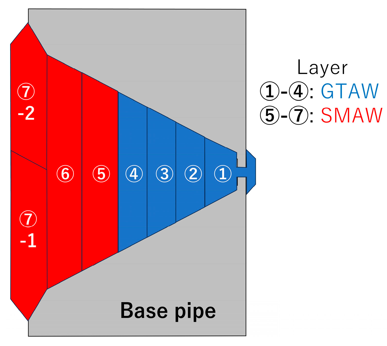
2.1. Test Material

The test material was a welded joint in SUS316 piping. The base pipe was solution-annealed at 1060 °C after fabrication, and then water quenched. The joint featured a bevel angle of 60° and consisted of seven layers. The first layer was executed using gas tungsten arc welding (GTAW) with a stainless steel (JIS YS316L) insert ring. Layers 2 to 4 were fabricated using GTAW with stainless steel (JIS YS316L) welding wire. Layers 5 to 7 were constructed using shielded metal arc welding (SMAW) with a stainless steel (JIS ES316-16) welding rod, with the seventh layer being welded in two passes. Figure 1 presents a schematic diagram of the welded section. This combination of GTAW and SMAW represents one of the standard methodologies for welding medium-diameter stainless steel piping in nuclear fields. The heat input ranged from 10–20 kJ/cm for GTAW to 30–40 kJ/cm for SMAW. The excess weld metal and adjacent outer surface areas were smoothened through grinding and polishing. The base pipe had an outer diameter of 165.2 mm, a wall thickness of 14.3 mm, and a length of 200 mm. The thickness at the center of the weld line was approximately 15 mm, tapering to about 13 mm at positions 60 mm from the center due to the thinning process. The chemical compositions of the base metal and the weld materials are detailed in

Table 1. Chemical compositions of the base pipe and weld materials (mass%).

Element	C	Si	Mn	P	S	Ni	Cr	Mo	Cu	Fe
Base pipe	0.05	0.37	1.43	0.033	0.004	10.25	16.53	2.06	-	Bal.
Insert ring	0.012	0.36	1.78	0.023	0.001	12.09	19.44	2.36	0.27	Bal.
GTAW	0.017	0.41	1.88	0.005	0.002	11.38	19.61	2.31	0.01	Bal.
SMAW	0.055	0.41	1.40	0.029	0.009	12.08	19.22	2.33	0.26	Bal.

. A section near the weld line was removed using electrical discharge machining (EDM) to facilitate neutron diffraction measurements. Additionally, strain-free d₀ specimens, each 2 mm thick in the hoop direction of the pipe, and a plate specimen for the DEM measurements, 5 mm thick in the hoop direction, were also procured from this section via EDM. Figure 2 and Figure 3 show a schematic diagram and a photograph of the test material, respectively.

2.2. Specimens

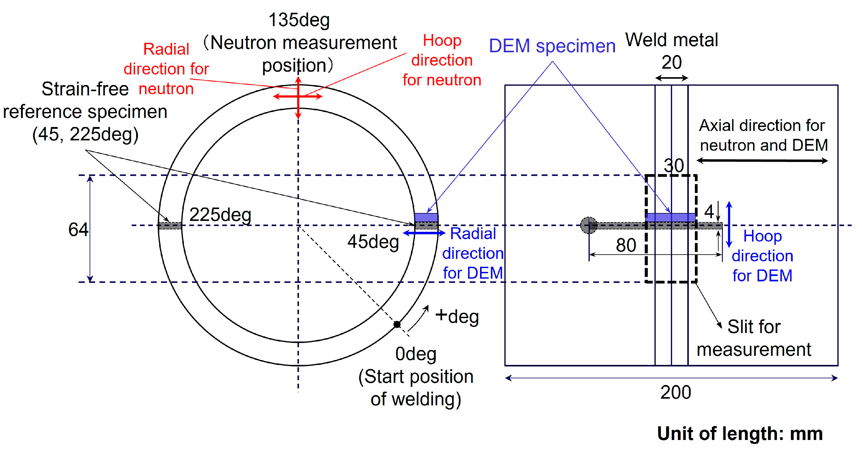
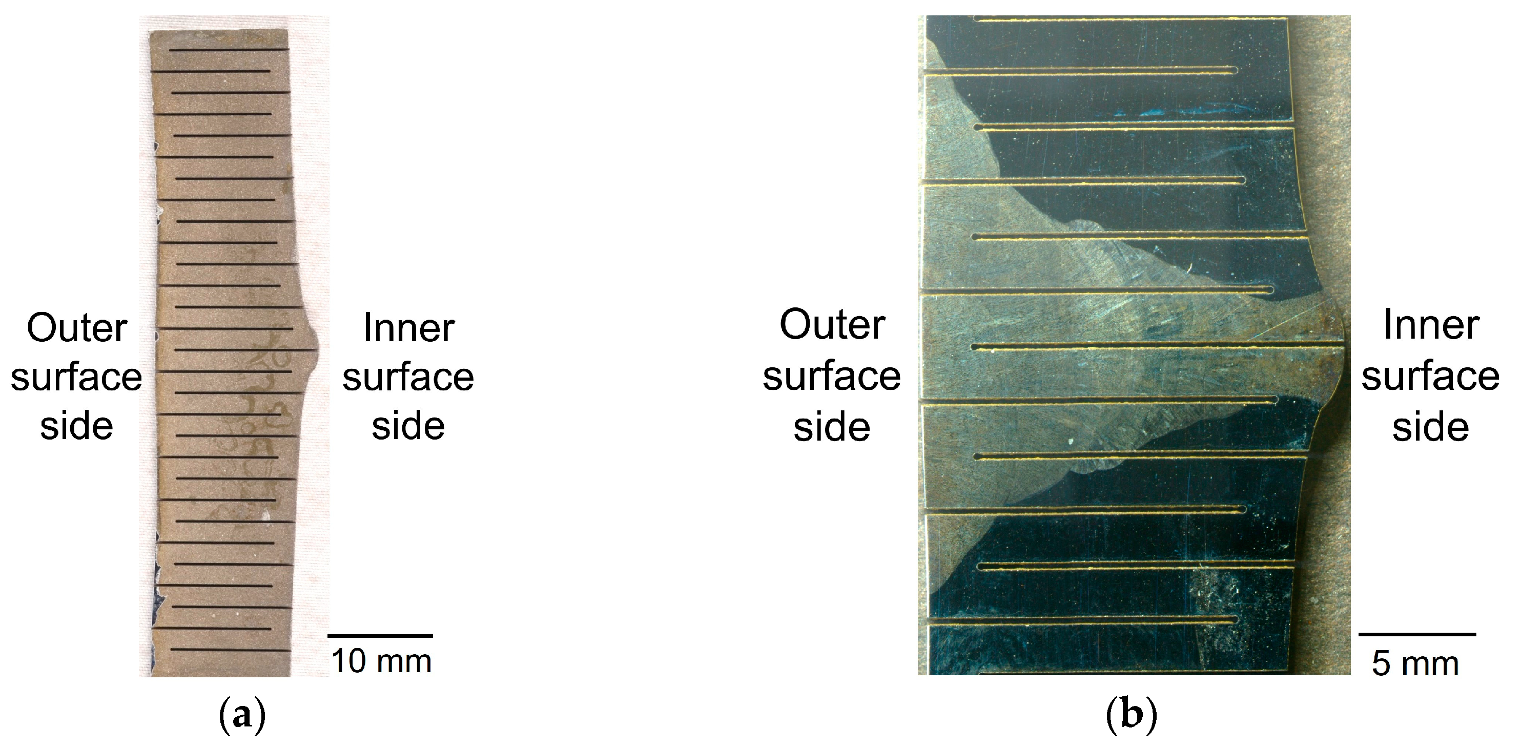
2.2.1. Strain-Free Reference Specimen

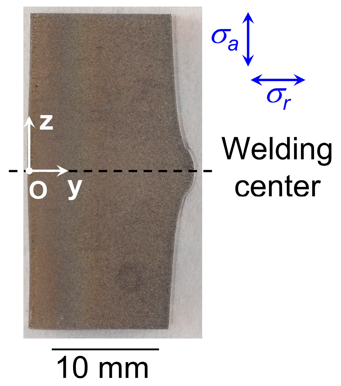
For the strain scanning method, it is necessary to prepare a specimen capable of assuming a strain-free state. Specimens with a thickness of 2 mm in the hoop direction of the pipe were extracted at angles of 45° and 225° utilizing wire-cut EDM. The elastic strain in these specimens was mitigated by cutting alternating slits from the inner and outer surfaces at 2 mm intervals using wire-cut EDM. These slits were then aligned and assembled to create a strain-free reference specimen with an overall thickness of 4 mm for subsequent measurements. The strain-free reference specimen is depicted in Figure 4. It is well-documented that weld metal in austenitic stainless steels typically contains a small fraction of δ-ferrite [19]. Microstructural analysis of a specimen obtained from the weld metal of the welded pipe confirmed the presence of approximately 8% δ-ferrite.

2.2.2. DEM Specimen

The specimen for the double-exposure method (DEM) was prepared from a section at a 45° angle of the welded pipe specimen. This specimen was designed with dimensions of 5 mm in the hoop direction and 29.5 mm in the axial direction of the pipe. Its thickness in the radial direction was maintained equal to that of the pipe itself. Figure 5 features a photograph of the DEM specimen. In this image, the vertical center aligns with the center of the weld line, the left side represents the outer surface of the pipe, and the right side indicates the inner surface. Given that the thickness of this specimen was limited to 5 mm, it was presumed that the hoop stress within it would be zero.

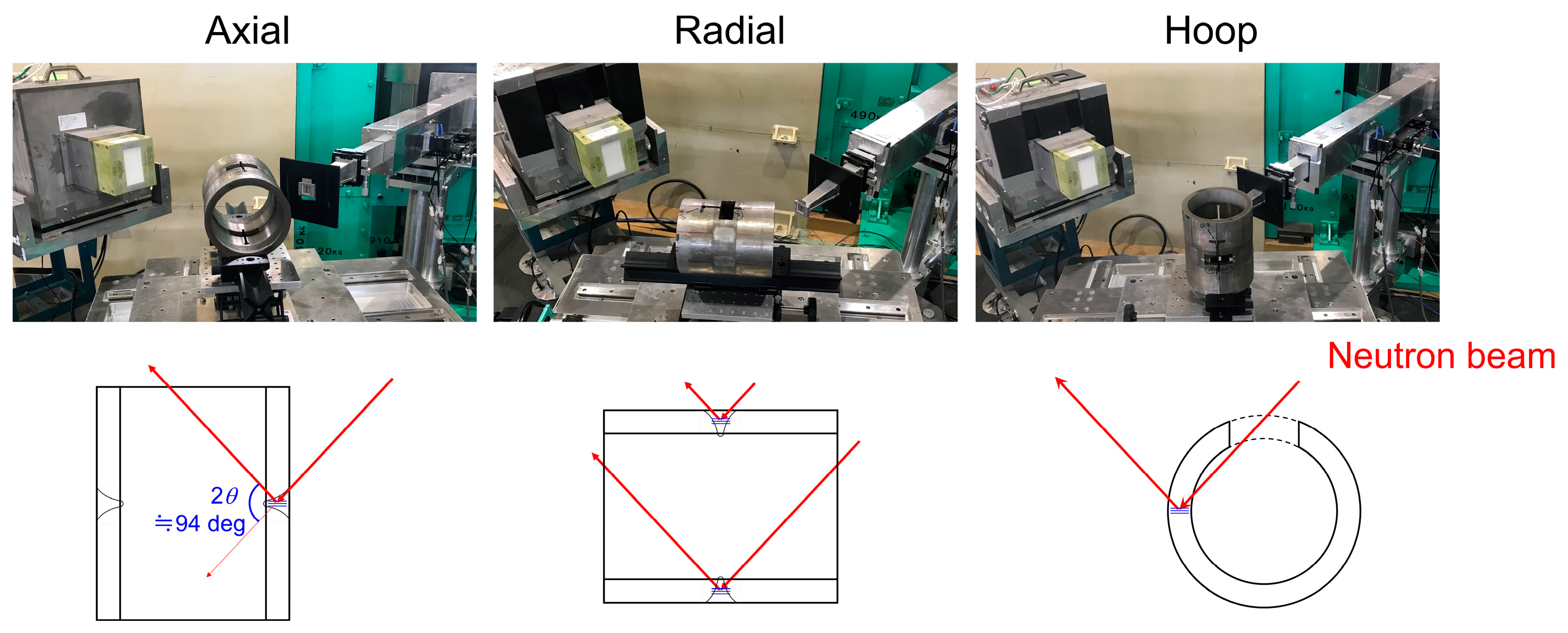
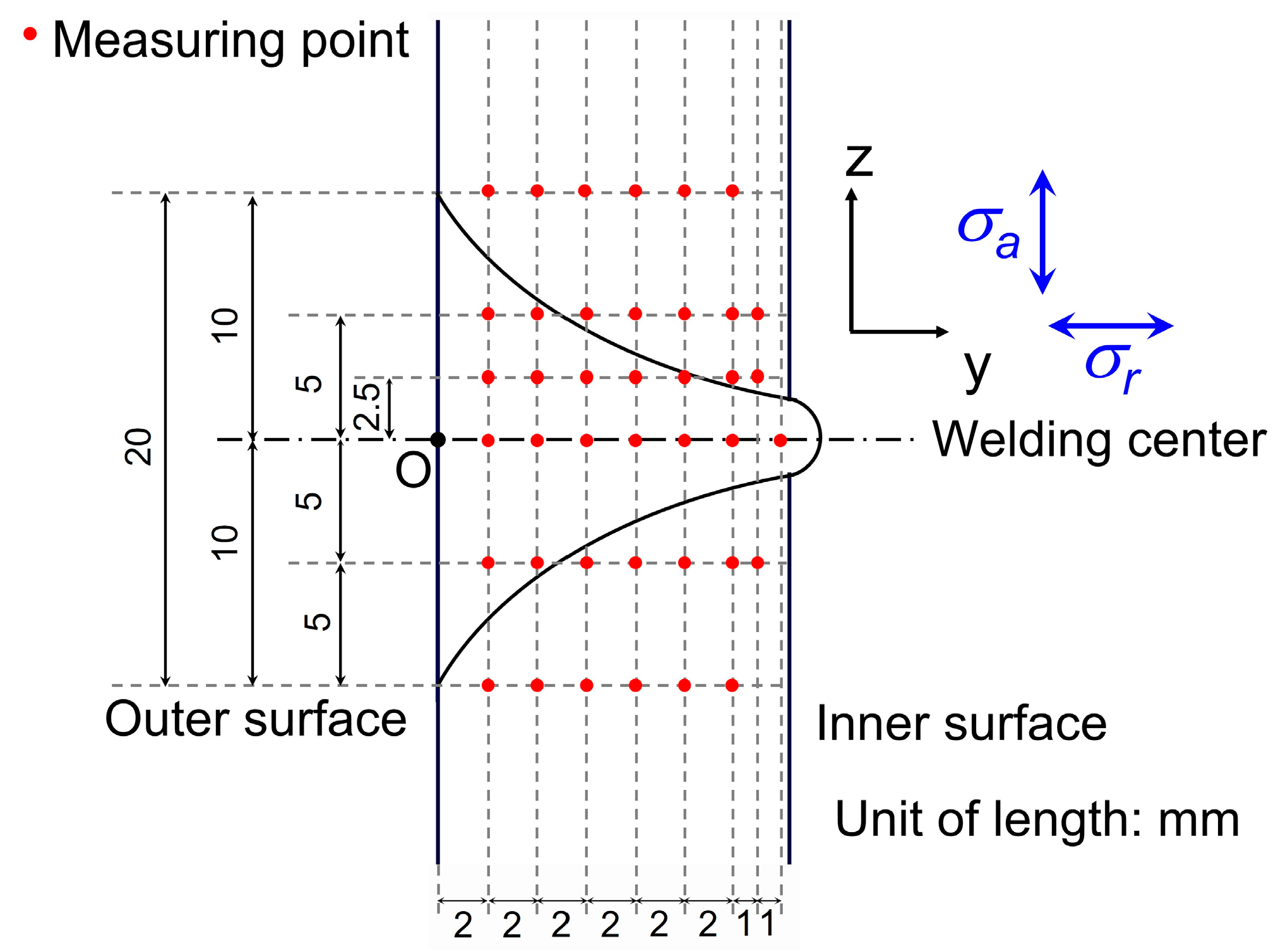
2.3. Neutron Stress Measurements

The thermal neutron flux emanating from Japan Research Reactor No. 3 (JRR-3) underwent monochromatization via a monochromator, culminating in extracting a neutron beam characterized by a wavelength of λ = 1.591 Å, tailored for these measurements. Stress assessments were conducted using the 311 diffractions from the γ-Fe and strain scanning methodology [8]. Data acquisition employed a one-dimensional 3He detector equipped with a 2 mm radial collimator on the detector side, facilitating the determination of the gauge volume. Diffraction patterns were derived by segregating and enumerating the diffracted neutrons through a 256-channel multichannel analyzer and subsequently approximated using a Gaussian function to determine the diffraction angle, 2θ. Photographs and schematic illustrations of the experimental setup for the neutron diffraction measurements are shown in Figure 6. These evaluations were primarily focused around a 135° angle, with specific measurement locations detailed in Figure 7. The strain was measured at each point in three orientations: axial, radial, and hoop. The slit dimensions were set at 2 mm width × 15 mm height for measurements in both axial and radial directions and 3 mm width × 3 mm height for the hoop direction. Consequently, the nominal gauge volume for measurements in the axial and radial directions assumed a prismatic shape elongated in the hoop direction. For the strain-free reference specimen, the slit dimensions were set to 2 mm width × 2 mm height in three orientations.

The elastic strain, ε, at each measurement point was calculated from the following equation using the lattice spacing, d, at each measurement point and the strain-free lattice spacing, d₀, which were calculated using Bragg’s law and the diffraction angle, 2θ:

$$\epsilon =\frac{d-d_0}{d_0}.$$

(1)

The axial stress, σ_a, radial stress, σ_r, and hoop stress, σ_h, were obtained from the axial strain, ε_a, radial strain, ε_r, and hoop strain, ε_h, respectively, using the following equations:

$${\sigma }_{\mathrm{a}}=\frac{E}{1+v}\left[{\epsilon }_{\mathrm{a}}+\frac{v}{1-2v}\left({\epsilon }_{\mathrm{a}}+{\epsilon }_{\mathrm{h}}+{\epsilon }_{\mathrm{r}}\right)\right],$$

(2)

$${\sigma }_{\mathrm{r}}=\frac{E}{1+v}\left[{\epsilon }_{\mathrm{r}}+\frac{v}{1-2v}\left({\epsilon }_{\mathrm{a}}+{\epsilon }_{\mathrm{h}}+{\epsilon }_{\mathrm{r}}\right)\right],$$

(3)

$${\sigma }_{\mathrm{h}}=\frac{E}{1+v}\left[{\epsilon }_{\mathrm{h}}+\frac{v}{1-2v}\left({\epsilon }_{\mathrm{a}}+{\epsilon }_{\mathrm{h}}+{\epsilon }_{\mathrm{r}}\right)\right].$$

(4)

The diffraction elastic constant, E, and Poisson’s ratio, ν, for the 311 lattice planes of SUS316 single crystals were determined to be 182.5 GPa and 0.307, respectively. These values were calculated using the Kröner model [20], incorporating elastic stiffness values of c₁₁ = 206 GPa, c₁₂ = 133 GPa, and c₄₄ = 119 GPa [21]. The strain-free lattice spacing, d₀, was measured using a reference specimen; this measurement was conducted at z = 0 for the weld metal and at z = −10 for the base metal. Given that the variance in lattice spacing at each measurement point was relatively small and no significant directional dependence was observed, the average of all measured d₀ values was designated as d₀ for this study. The mean value of d₀ across all measurement points was 1.08471 Å, with a standard deviation of 1.3 × 10⁻⁴ Å. The stress range corresponding to this standard deviation, as calculated using the diffraction elastic constant, E, was found to be 23.7 MPa.

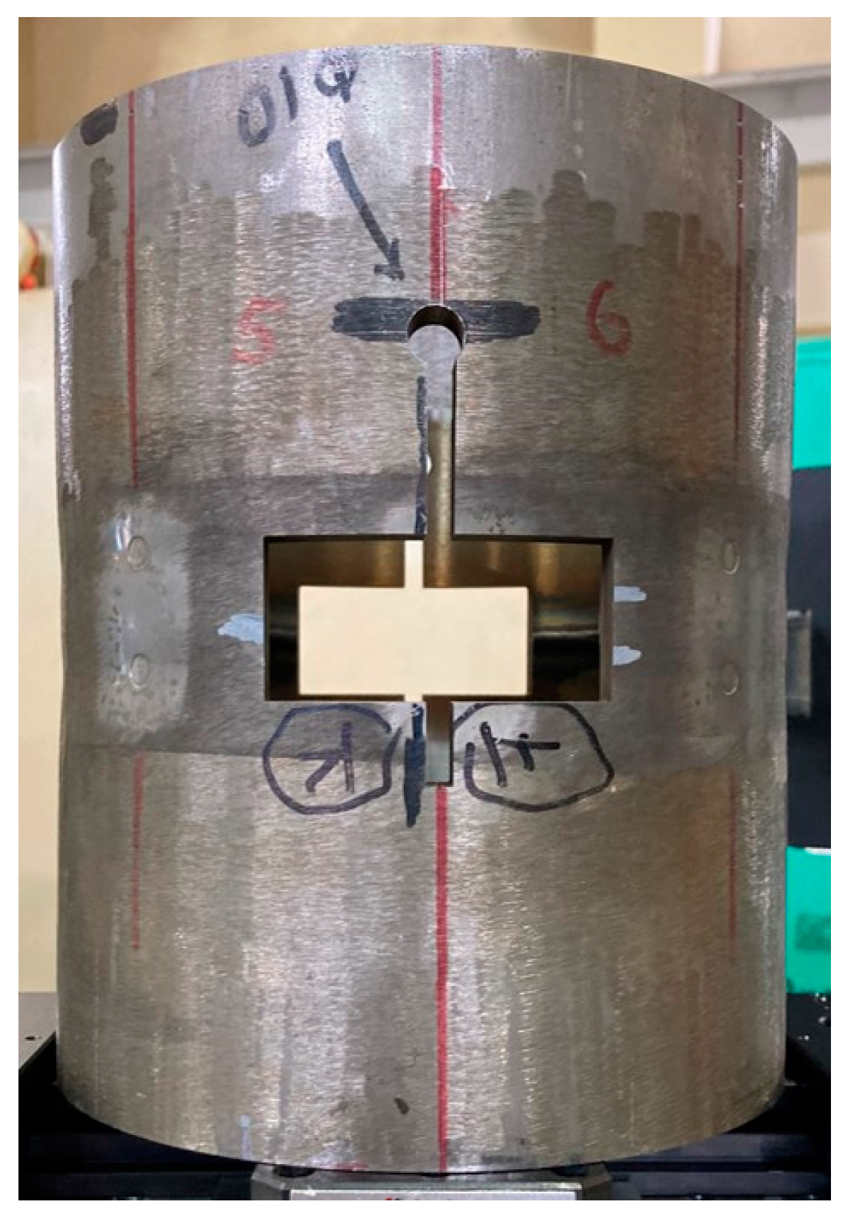
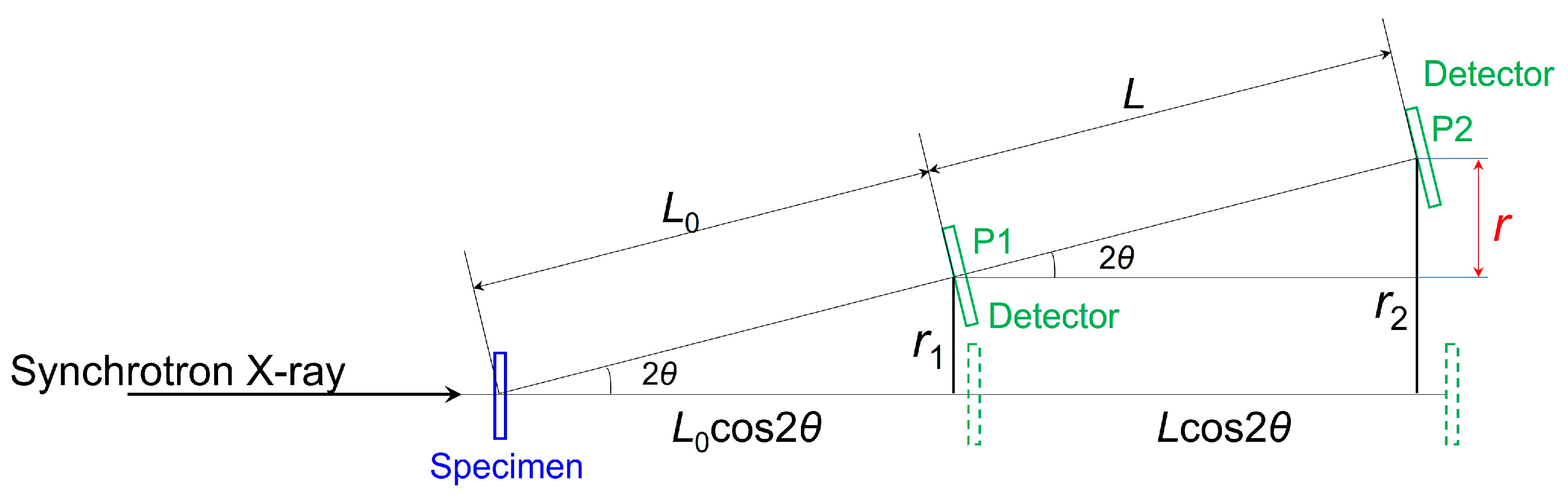
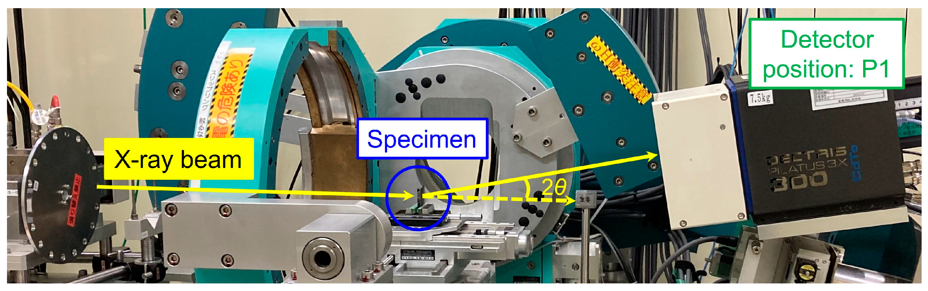
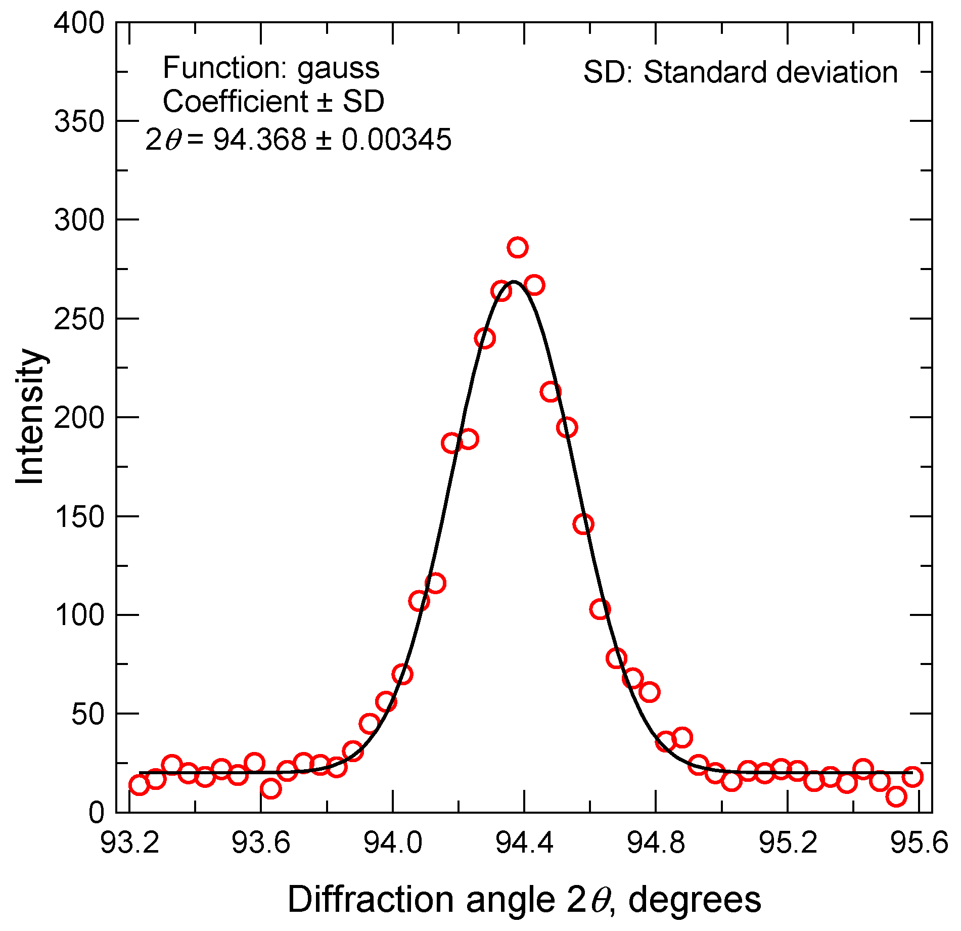
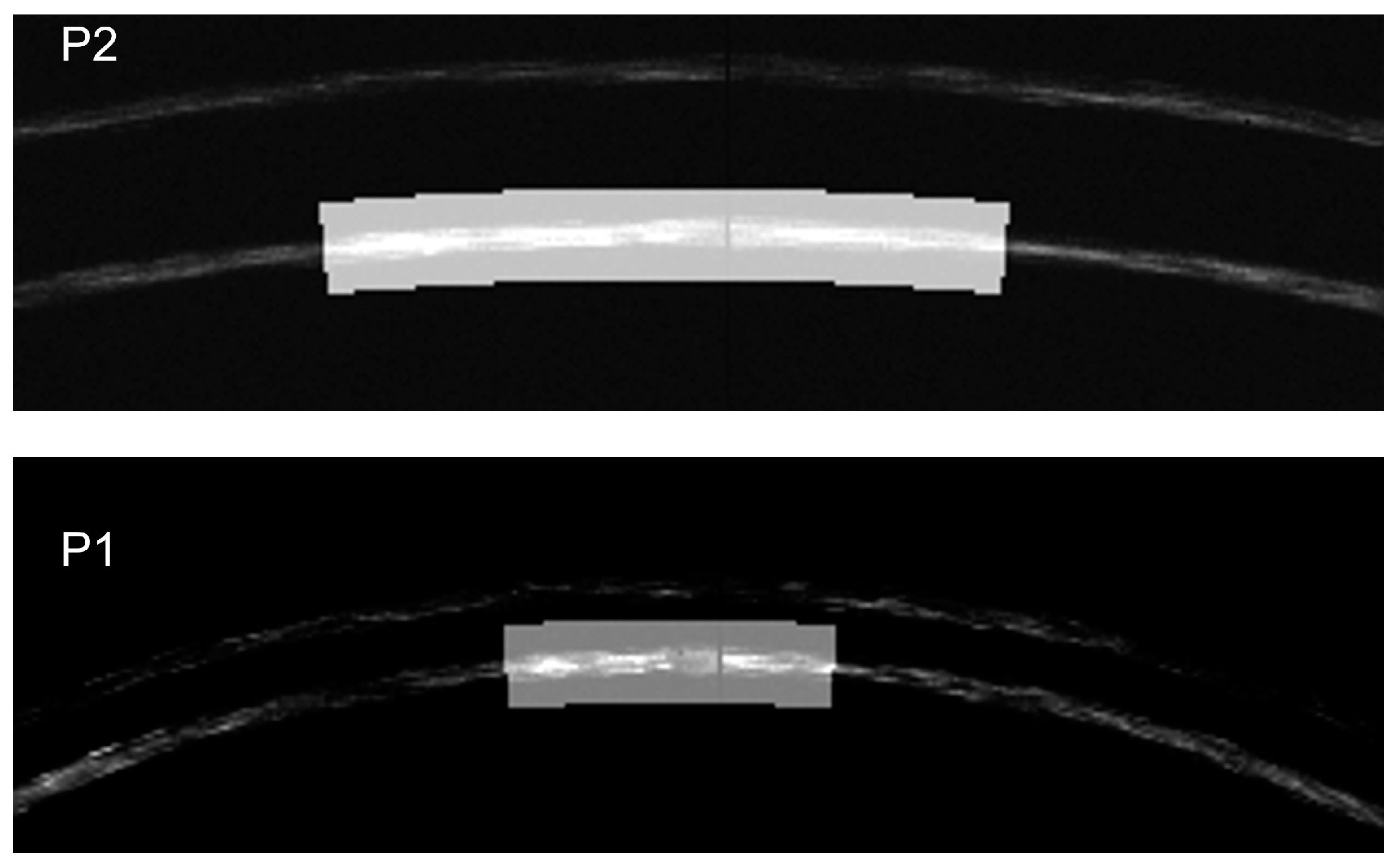
2.4. DEM with Synchrotron X-rays

Stress measurements were conducted using high-energy synchrotron radiation at the BL16XU beamline of SPring-8, employing an X-ray energy of 71.92 keV. The X-ray beam was shaped to 0.4 mm × 0.4 mm. The diffraction patterns were acquired using a PILATUS CdTe 300 K detector (Dectris Ltd., 5405 Baden-Daettwil, Switzerland), a two-dimensional detector installed on the 2θ arm of the diffractometer at BL16XU. The detector area was 83.8 mm × 106.5 mm, consisting of 487 × 619 pixels, each measuring 0.172 mm × 0.172 mm. The 2θ arm angle of the diffractometer was set to 9° to align with the diffraction angle of the 311 lattice planes at this X-ray energy. Measurements were performed in the axial and radial directions of the pipe, corresponding to the z and y axes, as shown in Figure 5.

Figure 8 presents a schematic diagram of the experimental setup during the DEM measurements. The X-ray beam passed through the DEM specimen, with diffracted X-rays detected vertically. Strain in the axial and radial directions of the pipe was measured by rotating the specimen 90° using the χ-cradle of the diffractometer. The detector positions labeled P1 and P2 were achieved by moving the detector on the 2θ arm by a distance of L, capturing diffraction patterns at both positions. The distance, L₀, between the specimen and P1 was 450 mm, while the distance, L, from P1 to P2 was 500 mm. Figure 9 displays a photograph of the experimental arrangement for the DEM measurements at detector position P1.

The diffraction radii, r₁ and r₂, were determined from the diffraction images measured at P1 and P2, respectively, and the diffraction radius, r, was calculated from the difference between r₂ and r₁, that is, r = r₂ − r₁. As shown in Figure 8, the diffraction angle, 2θ, can be expressed as follows:

$$2\theta ={\sin }^{-1}\left(\frac{r}{L}\right).$$

(5)

The effect of the diffracting crystal grains’ positions within the specimen is canceled out by the definition of r, allowing for the acquisition of the diffraction angle, 2θ, without influence from the diffraction position. The coordinates for the DEM measurement are detailed in

Table 2. DEM measurement coordinates (the y and z directions are indicated in Figure 5).

y Range (0.4 mm Pitch)	z Range (1.0 mm Pitch)
0.4~12.8	−7~−5, 6~10
0.4~14.0	−4~−2, 2~5
0.4~14.8	−1, ~1

. While DEM analysis necessitates a stress-free reference lattice spacing, d₀, for the computation of elastic strain and stress, the lattice spacing deduced from the diffraction angle, 2θ, which in turn is derived from the diffraction pattern acquired by scanning from the inner to the outer surface at the z = 14 mm position, was defined as d₀. This spacing has been subsequently utilized in the strain calculation.

3. Results and Discussion

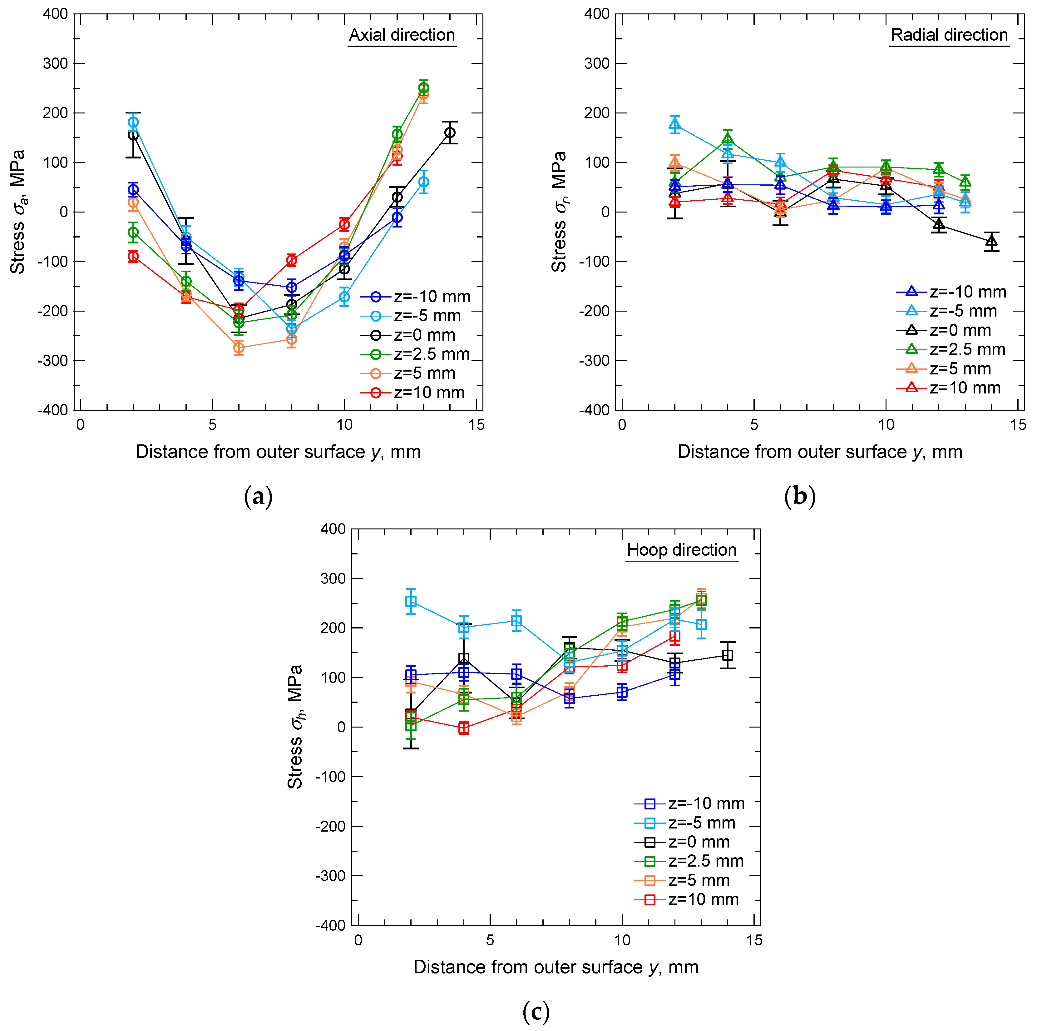
3.1. Residual Stress Distribution Measured by Neutron Diffraction

A typical diffraction pattern and Gaussian fitting result of the neutron measurement are shown in Figure 10. In this study, we defined the residual stress error, Δσ, as the value calculated from Equations (2)–(4) using the residual strain error, Δε, expressed as follows:

$$\left|∆\epsilon \right|=\left|\frac{∆d}{d_0}\right|.$$

(6)

The residual strain error, Δε, was determined from the lattice spacing error, Δd, which was itself derived from the standard deviation of the diffraction angle, Δ2θ, ascertained through Gaussian fitting.

Figure 11 illustrates the stress distributions in the axial, radial, and hoop directions across the thickness of the welded pipe specimen. A consistent axial stress pattern was observed at all measurement locations, characterized by a decrease in stress from tension on the inner surface side towards the central area, followed by an increase towards the outer surface. In the weld heat-affected zone (HAZ), the axial stress on the inner surface side tended to diminish with increasing distance from the weld line, aligning with the reported FEM analysis results [11]. Figure 12 shows triaxial stress maps, which were developed from the data presented in Figure 11 and superimposed onto the DEM specimen. These maps were generated by designating each measurement point as a grid point and applying linear interpolation between these points. The maps revealed a relatively high tensile stress near the boundary between the weld metal and the HAZ on the inner surface of the pipe, correlating with the SCC initiation point observed in actual PLR piping of BWRs [1]. The stress distribution exhibited asymmetry relative to the weld line, potentially since the seventh layer of welding was performed using two-pass welding.

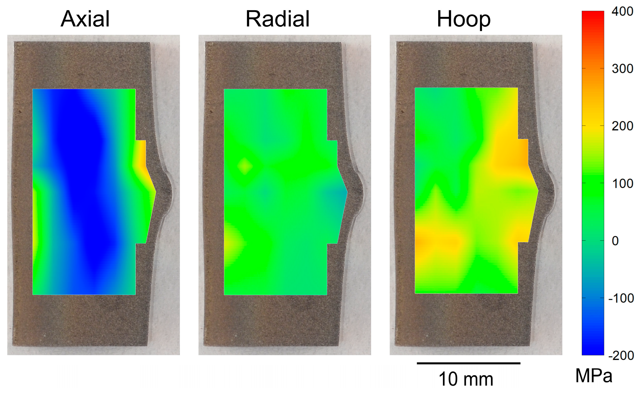
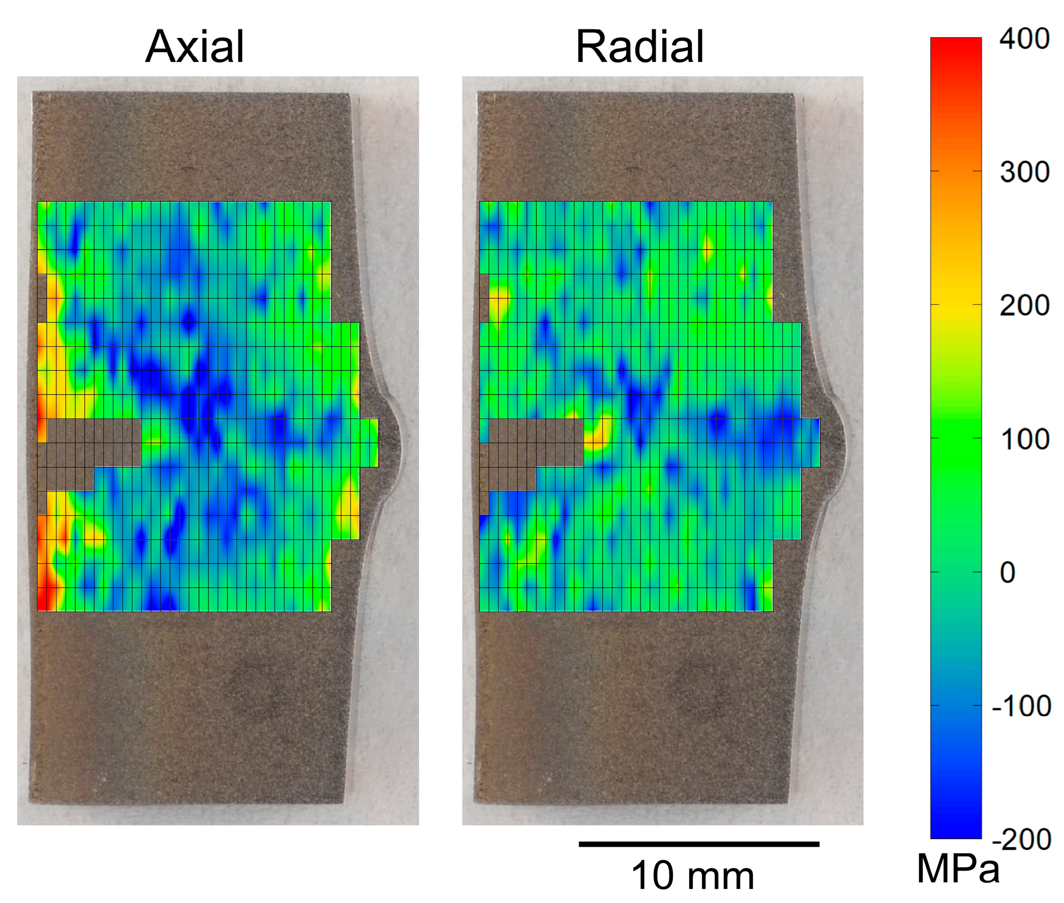
3.2. 2D Stress Distributions Measured by DEM

Representative diffraction images from the specimen, acquired at detector positions P1 and P2, are illustrated in Figure 13. The bright areas in this figure denote the regions where integration was conducted to derive the diffraction curves. In these measurements, it is not possible to acquire a continuous diffraction ring due to the small beam size relative to the grain size. As depicted, the ring is discontinuous in both circumferential and radial directions, exhibiting non-uniform contrast. This discontinuity results from the presence of large dendrites and a limited number of crystal grains within the beam path. For most X-ray diffraction methods, accurately determining the diffraction angle, 2θ, from such a discontinuous ring presents a challenge. On the other hand, the similarity of the diffraction images within the integration areas of P1 and P2 is obvious. Given that the DEM technique leverages the difference between two diffraction images, it becomes feasible to ascertain the diffraction angle, 2θ, from these discontinuous images. Regarding the diffraction images captured at P1 and P2, the correlation between the diffraction radius and intensity was obtained through circumferential integration across a ±5° range centered around the beam. This data was then approximated using a Gaussian function, enabling the calculation of the diffraction radii, r₁ and r₂, at P1 and P2, respectively. Subsequently, the diffraction angle, 2θ, was deduced using Equation (5).

Since the strain obtained from Equations (1) and (5) is the value in the direction tilted by θ from the in-plane direction of the specimen, the strain in the in-plane direction was obtained using the following equations [17]:

$${\sigma }_{\mathrm{a}}=\frac{E}{\left(1+v\right){\cos }^2\theta }\left[{{\epsilon }_{\mathrm{a}}}^{\prime }+S^{\prime }\left({{\epsilon }_{\mathrm{a}}}^{\prime }+{{\epsilon }_{\mathrm{r}}}^{\prime }\right)\right],$$

(7)

$${\sigma }_{\mathrm{r}}=\frac{E}{\left(1+v\right){\cos }^2\theta }\left[{{\epsilon }_{\mathrm{r}}}^{\prime }+S^{\prime }\left({{\epsilon }_{\mathrm{a}}}^{\prime }+{{\epsilon }_{\mathrm{r}}}^{\prime }\right)\right],$$

(8)

$$S^{\prime }=\frac{v}{\left(1+v\right){\cos }^2\theta -2v} ,$$

(9)

where ε_a^′ and ε_r^′ are the axial and radial strains tilted by θ from the in-plane direction of the specimen, respectively, and E and ν are as defined above. The axial stress, σ_a, and radial stress, σ_r, were obtained using Equations (7)–(9) assuming a plane stress state. Residual stress maps of the DEM specimen created by linearly complementing the measured values as grid points are shown in Figure 14. In these measurements, there were some measurement points in the SMAW weld metal with coarse grains, where no diffraction image could be obtained within the circumferential integration region and strain measurement could not be performed. In such cases, the region without values around the measurement point is omitted.

In this measurement, the residual stress error was calculated from Δr and expressed as follows:

$$∆r=\sqrt{∆r_1{}^2+∆r_2{}^2}.$$

(10)

Δr₁ and Δr₂ are the standard deviations of r₁ and r₂ determined by Gaussian fitting, respectively. The error range calculated using Equations (5)–(10) was about ±15 MPa on average in both the axial and radial directions and about ±40 MPa at points with low peak determination accuracy by Gaussian fitting.

Although the gauge volume and measurement location differ between the strain scanning method using neutrons and the DEM, the overall stress distributions were relatively similar. These distributions are characterized by axial stress decreasing from tension on the inner surface side toward the center and then increasing again towards the outer surface side. The DEM provided superior spatial resolution compared to neutron diffraction, enabling measurements close to the inner surface of the pipe weld. This capability is crucial for evaluating SCC initiation and propagation. However, the axial tensile stress observed on the inner surface of the pipe with DEM was not as high as that detected by neutron diffraction. This discrepancy is likely due to the relaxation of hoop stress during the slicing process in DEM specimen preparation.

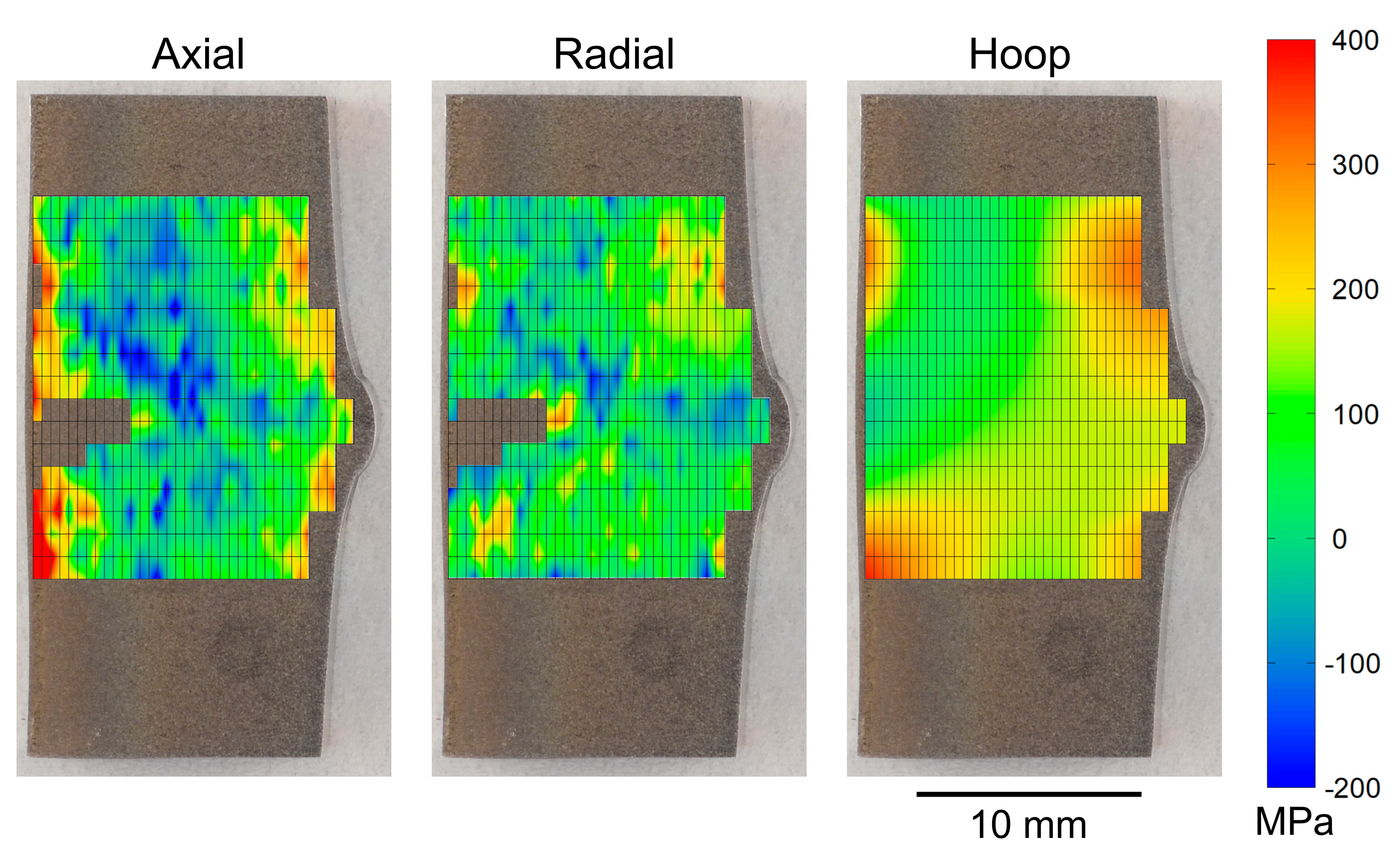
3.3. Evaluation of Triaxial Residual Stress by Combination of Neutron Diffraction and DEM

To estimate the pre-relaxation stress distribution in the residual stress distribution maps measured by DEM, we utilize a method based on the hoop stress distribution obtained through neutron diffraction. This method involves approximating the hoop stress distribution, as presented in Figure 11, as a cubic function of the normalized distance from the outer surface, represented by y/t, where t denotes the pipe thickness at each ‘z’ position. Under the assumption that the coefficients a, b, c, and d can be described as quartic functions of the distance z, we derive the following equation:

$$\begin{gathered} {\sigma }_{\mathrm{h}\left(y, z\right)}=a{\left(\frac{y}{t}\right)}^3+b{\left(\frac{y}{t}\right)}^2+c\frac{y}{t}+d, \\ a=0.3341z^4+1.418z^3-34.07z^2+254.2z+164.0, \\ b=-0.9267z^4-2.462z^3+98.30z^2+429.7z-537.9, \\ c=0.6901z^4+0.9443z^3-75.11z^2-167.7z+589.1, \\ d=-0.1530z^4+0.07210z^3+16.35z^2-4.224z-42.68. \end{gathered}$$

(11)

Next, we assume that the axial and radial strains of the DEM specimen obtained under the plane stress condition are subject to the hoop stress, σ_h(y,z), in Equation (11) under the plane strain condition. The axial strain, ε_{a_DEM}, and radial strain, ε_{r_DEM}, obtained from Equations (7)–(9) assuming a plane stress state can be expressed by the following equations:

$${\epsilon }_{\mathrm{a}\_\mathrm{DEM}}=\frac{1}{E}\left({\sigma }_{\mathrm{a}\_\mathrm{DEM}}-v{\sigma }_{\mathrm{r}\_\mathrm{DEM}}\right),$$

(12)

$${\epsilon }_{\mathrm{r}\_\mathrm{DEM}}=\frac{1}{E}\left({\sigma }_{\mathrm{r}\_\mathrm{DEM}}-v{\sigma }_{\mathrm{a}\_\mathrm{DEM}}\right),$$

(13)

where E and ν are the same elastic constant and Poisson’s ratio defined above. On the other hand, under the plane strain state, ε_a and ε_r can be expressed by the following equations:

$${\epsilon }_{\mathrm{a}}=\frac{1}{E}\left\{{\sigma }_{\mathrm{a}}-v\left({\sigma }_{\mathrm{r}}+{\sigma }_{\mathrm{h}}\right)\right\},$$

(14)

$${\epsilon }_{\mathrm{r}}=\frac{1}{E}\left\{{\sigma }_{\mathrm{r}}-v\left({\sigma }_{\mathrm{a}}+{\sigma }_{\mathrm{h}}\right)\right\}.$$

(15)

By transforming Equations (14) and (15), the residual stresses under a triaxial stress state can be approximated by the following equations:

$${\sigma }_{\mathrm{a}}=\frac{E}{1-v^2}\left({\epsilon }_{\mathrm{a}\_\mathrm{DEM}}+v{\epsilon }_{\mathrm{r}\_\mathrm{DEM}}\right)+\frac{v}{1-v}{\sigma }_{\mathrm{h}\left(y, z\right)},$$

(16)

$${\sigma }_{\mathrm{r}}=\frac{E}{1-v^2}\left({\epsilon }_{\mathrm{r}\_\mathrm{DEM}}+v{\epsilon }_{\mathrm{a}\_\mathrm{DEM}}\right)+\frac{v}{1-v}{\sigma }_{\mathrm{h}\left(y, z\right)}.$$

(17)

Under the assumptions of this paper, the stresses calculated by the equation may exceed the actual triaxial stresses. Nonetheless, considering the structural integrity assessment in relation to SCC, higher stress predictions yield conservative results and are thus deemed acceptable. Consequently, this method is validated as a simplified approach for triaxial stress evaluation in welded pipes.

Figure 15 shows residual stress maps, created similarly to Figure 14, utilizing stresses in three directions derived from Equations (11), (16), and (17). High axial stress around the HAZ near the inner surface and relatively high radial stress around the same HAZ were observed. These observations align with FEM analysis results reported in the literature [11]. Additionally, the residual stress maps suggest that SCC initiated at the HAZ tends to propagate towards the weld metal, a phenomenon corroborated by observations of the PLR piping of BWRs [1]. While extremely high tensile stresses near the outer surface are noticeable in Figure 15, these could be attributed to the grinding process during the welded pipe’s fabrication. These results demonstrate that combining the DEM with neutron diffraction can uncover the residual stress distribution in the thickness direction with high spatial resolution. This includes the weld metal, which is typically challenging to measure using X-ray diffraction methods. The proposed method holds promise not only for measuring residual stresses in various welds but also for validating welding residual stress evaluation results obtained through numerical analysis, and such validations could also contribute to the advancement of numerical analysis methodologies.

4. Conclusions

In this study, we introduced a method for assessing the triaxial stress distribution in stainless steel piping welds by synergistically utilizing high-energy synchrotron X-ray radiation and neutron diffraction. The conclusions drawn from this research are as follows:

• The DEM is an effective tool for stress evaluation in welds and coarse grains using high-energy synchrotron X-rays. Its effectiveness is primarily due to its low susceptibility to errors arising from the diffraction positions of the coarse grains in the weld.
• Residual stresses in welded piping were quantified using the strain scanning method with neutron diffraction. The triaxial stress distribution, as determined by this method, was modeled using a polynomial equation, enabling the creation of a hoop stress map.
• The axial and radial stresses, obtained from the DEM using high-energy synchrotron X-ray radiation, were integrated with the hoop stresses measured via neutron diffraction. This integration, based on a plane strain assumption, facilitated the development of a comprehensive residual stress map for the weld in a triaxial stress state.

References

1. Suzuki, S.; Takamori, K.; Kumagai, K.; Sakashita, A.; Yamashita, N.; Shitara, C.; Okumura, Y. Stress Corrosion Cracking in Low Carbon Stainless Steel Components in BWRs. E-J. Adv. Maint. 2009, 1, 1–29. [Google Scholar]
2. JSME S NAI-2020; Codes for Nuclear Power Generation Facilities—Rules on Fitness-for-Service for Nuclear Power Plants. Japan Society of Mechanical Engineers: Tokyo, Japan, 2020.
3. Rudland, D.; Harrington, D.; Dingreville, R. Development of the Low Probability of Rupture (xLPR) Version 2.0 Code. In Proceedings of the ASME Pressure Vessel and Piping Conference PVP2015, PVP2015-45134, Boston, MA, USA, 19–23 July 2015. [Google Scholar]
4. Homiack, M.; Facco, G.; Benson, M.; Erikcson, M.; Harrington, C. Extremely Low Probability of Rupture Version 2 Probabilistic Fracture Mechanics Code; NUREG-2247; U.S. Nuclear Regulatory Commission: Washington, DC, USA, 2021; p. 20555-0001. [Google Scholar]
5. Mano, A.; Yanaguchi, Y.; Katsuyama, J.; Li, Y. Improvement of Probabilistic Fracture Mechanics Analysis Code PASCAL-SP with Regards to PWSCC. J. Nucl. Eng. Radiat. Sci. 2019, 5, 31501. [Google Scholar] [CrossRef]
6. Machida, H.; Arakawa, M.; Yamashita, N.; Yoshimura, S. Development of Probabilistic Fracture Mechanics Analysis Code for Pipes with Stress Corrosion Cracks. J. Power Energy Syst. 2009, 3, 103–113. [Google Scholar] [CrossRef]
7. JSMS-SD-5-02; Standard Method for Stress Measurement—Steels. The Society of Materials Science: Kyoto, Japan, 2005.
8. Allen, A.J.; Hutchings, M.T.; Windsor, C.G.; Andreani, C. Neutron diffraction methods for study of residual stress fields. Adv. Phys. 1985, 34, 445–473. [Google Scholar] [CrossRef]
9. Suzuki, H.; Katsuyama, J.; Tobita, T.; Morii, Y. Residual stress measurement of large scaled welded pipe using neutron diffraction method—Effect of SCC crack propagation and repair weld on residual stress distribution. Q. J. Jpn. Weld. Soc. 2011, 29, 294–304. [Google Scholar] [CrossRef]
10. Bouchard, P.J.; George, D.; Santisteban, J.R.; Bruno, G.; Dutta, M.; Edwards, L.; Kingston, E.; Smith, D.J. Measurement of the stresses in stainless steel pipe girth weld containing long and short repair. Int. J. Press. Vessel. Pip. 2005, 82, 299–310. [Google Scholar] [CrossRef]
11. Machida, H. Influence of Non-Destructive Examination Performance on Reliability of Pipes Having Stress Corrosion Cracks. Trans. JSME 2011, 77, 1798–1813. [Google Scholar] [CrossRef]
12. Maekawa, A.; Serizawa, H.; Nakacho, K.; Murakawa, H. Fast Finite Element Analysis of Weld Residual Stress in Larg-Diameter Thick-Walled Stainless Steel Pipe Joints and Its Experimental Validation. Q. J. Jpn. Weld. Soc. 2013, 31, 129s–133s. [Google Scholar] [CrossRef]
13. Dai, P.; Wang, Y.; Li, S.; Lu, S.; Feng, G.; Deng, D. FEM analysis of residual stress induced by repair welding in SUS304 stainless steel pipe butt-welded joint. J. Manuf. Process. 2020, 58, 975–983. [Google Scholar] [CrossRef]
14. George, D.; Smith, D.J. Through thickness measurement of residual stresses in a stainless steel cylinder containing shallow and deep weld repairs. Int. J. Press. Vessel. Pip. 2005, 82, 279–287. [Google Scholar] [CrossRef]
15. Hilson, G.; Simandjuntak, S.; Flewitt, P.E.J.; Hallam, K.R.; Pavier, M.J.; Smith, D.J. Spatial variation of residual stresses in a welded pipe for high temperature applications. Int. J. Press. Vessel. Pip. 2009, 86, 748–756. [Google Scholar] [CrossRef]
16. Suzuki, K.; Shiro, A.; Toyokawa, H.; Saji, C.; Shobu, T. Double-Exposure Method with Synchrotron White X-ray for Stress Evaluation of Coarse-Grain Materials. Quantum Beam Sci. 2020, 4, 25. [Google Scholar] [CrossRef]
17. Suzuki, K.; Kura, K.; Miura, Y.; Shiro, A.; Toyokawa, H.; Kajiwara, K.; Shobu, T. A study on Stress Measurement if Weld Part using Double Exposure Method. J. Soc. Mater. Sci. Jpn. 2022, 71, 1005–1012. [Google Scholar] [CrossRef]
18. Holmberg, J.; Steuwer, A.; Stormvinter, A.; Kristoffersen, H.; Haakanen, M.; Berglund, J. Residual stress state in an induction hardened steel bar determined by synchrotron and neutron diffraction compared to results from lab-XRD. Mater. Sci. Eng. A 2016, 667, 199–207. [Google Scholar] [CrossRef]
19. Chopra, O.K. Effects of Thermal Aging on Fracture Toughness and Charpy-Impact Strength of Stainless Steel Pipe Welds. NUREG/CR-6428, Rev. 1; U.S. Nuclear Regulatory Commission: Washington, DC, USA, 2018; p. 20555-0001. [Google Scholar]
20. Kröner, E. Berechnung der elastischen Konstanten des Vierkristalls aus den Konstanten des Einkristalls. Z. Physik 1958, 151, 504–518. [Google Scholar] [CrossRef]
21. Suzuki, K. X-ray and Mechanical Elastic Constants for Cubic System by Kröner Model. Available online: https://x-ray.jsms.jp/kroner/kroner_c.html (accessed on 16 May 2023).
Figure 1. Schematic diagram of the weld part of the pipe used in this study.
Qubs 08 00001 g001
Figure 2. Schematic diagram of the welded pipe test material.
Qubs 08 00001 g002
Figure 3. Photograph of the welded pipe test material (view from an angle of 225°).
Qubs 08 00001 g003
Figure 4. Strain-free reference specimen for neutron strain scanning: (a) photograph of the strain-free reference specimen, and (b) structure of the weld metal in the strain-free reference specimen.
Qubs 08 00001 g004
Figure 5. Photograph of the DEM specimen.
Qubs 08 00001 g005
Figure 6. Photographs and schematic diagrams of the experimental configuration used for the neutron diffraction measurements.
Qubs 08 00001 g006
Figure 7. Measurement points for the neutron diffraction measurements.
Qubs 08 00001 g007
Figure 8. Schematic diagram of the experimental configuration used for the DEM measurements.
Qubs 08 00001 g008
Figure 9. Photograph of the experimental setup used for the DEM measurements at detector position P1.
Qubs 08 00001 g009
Figure 10. Diffraction profile in radial direction at the measurement point of y = 2, z = −10.
Qubs 08 00001 g010
Figure 11. Stress distributions of the welded pipe specimen with respect to thickness: (a) axial direction, (b) radial direction, and (c) hoop direction.
Qubs 08 00001 g011
Figure 12. Welding residual stress maps of the welded pipe specimen measured by neutron diffraction.
Qubs 08 00001 g012
Figure 13. Representative diffraction images measured by the pixel detector at P1 and P2. The bright regions indicate the areas integrated to determine the diffraction angle, 2θ.
Qubs 08 00001 g013
Figure 14. Residual stress maps of the DEM specimen under the plane stress condition.
Qubs 08 00001 g014
Figure 15. Modified residual stress maps of the DEM specimen considering the hoop stress measured by neutron diffraction.
Qubs 08 00001 g015