
Experimental and Numerical Evaluation of Equivalent Stress Intensity Factor Models under Mixed-Mode (I+II) Loading
 , , , and
Abstract
:1. Introduction
2. Background
2.1. Equivalent SIF Models
2.2. Crack Growth Models
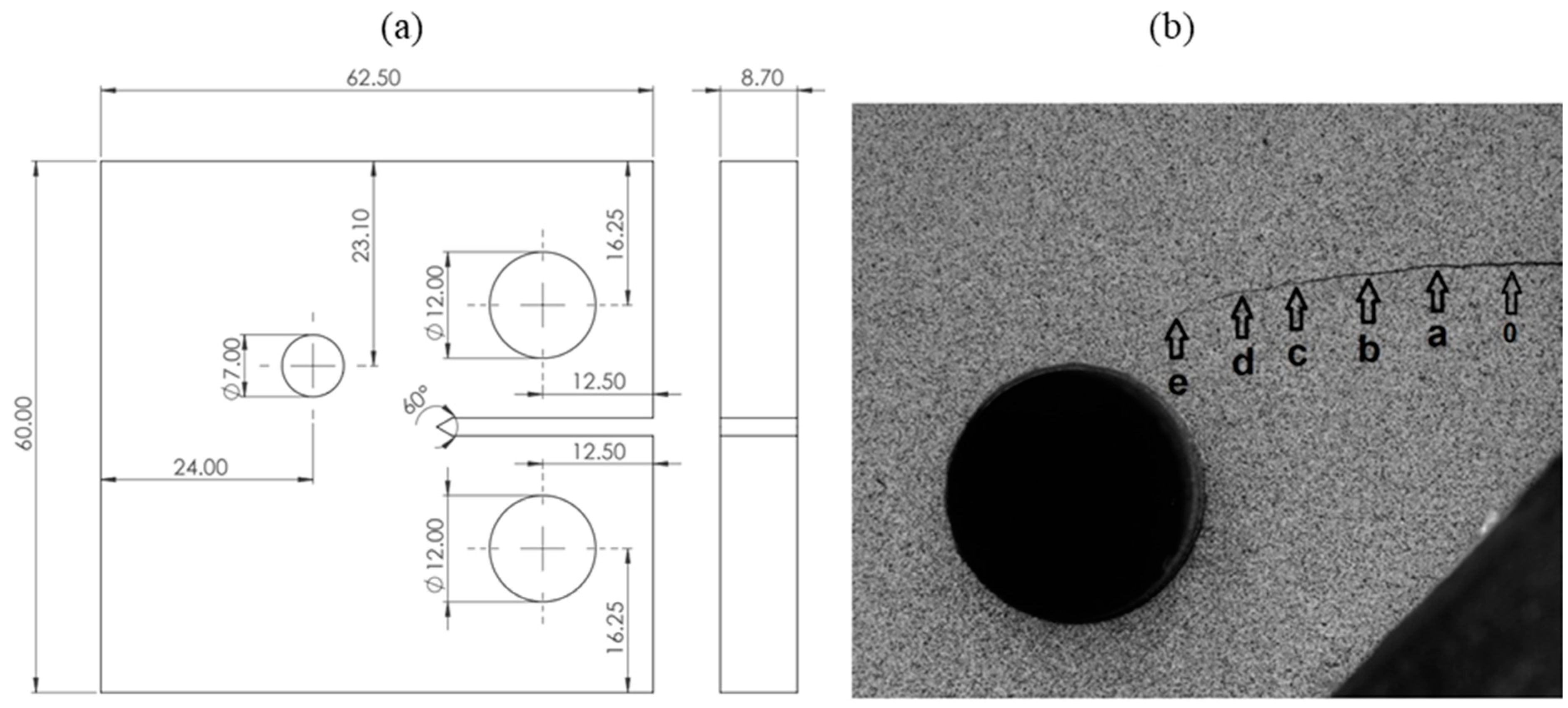
3. Materials and Methods
4. Results
4.1. Parametric Models
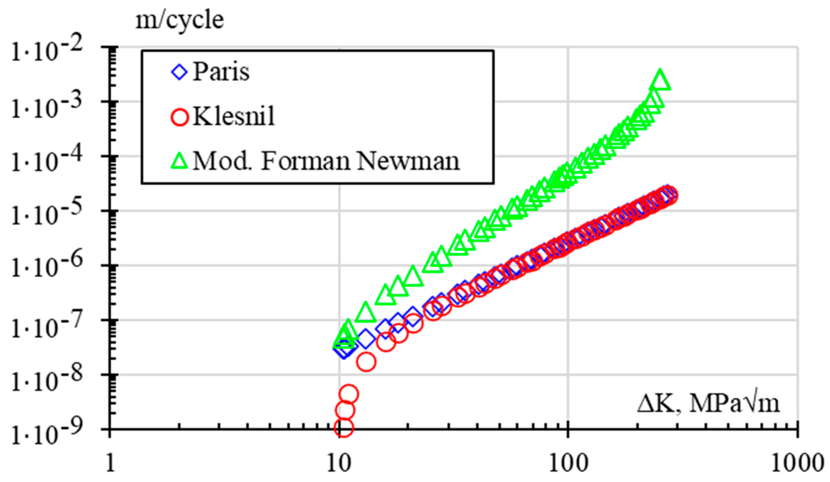
4.2. Paris Rule
4.3. Modified Forman Newman
4.4. Klesnil
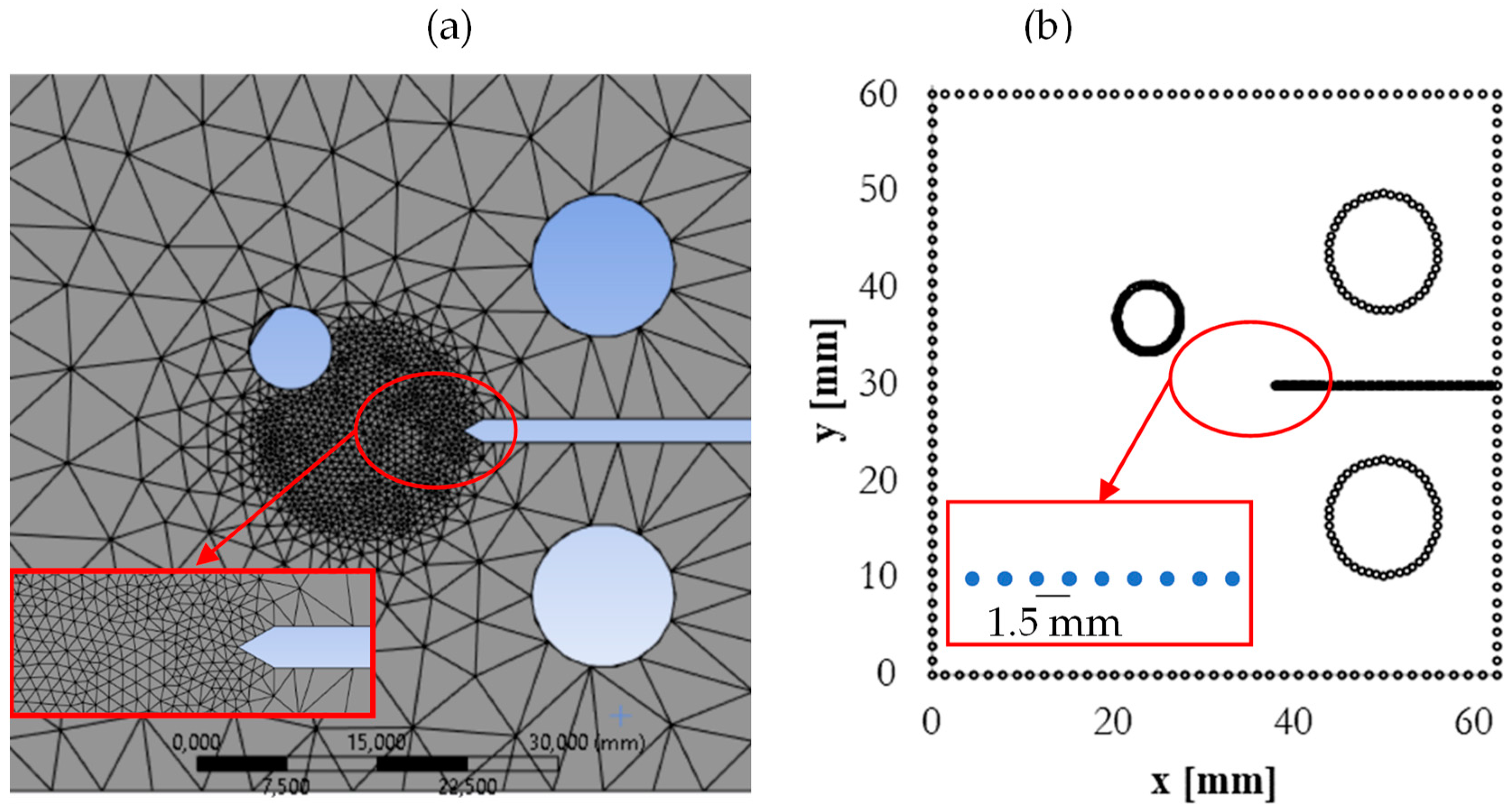
4.5. Numerical FEM
4.6. Numerical BEM
5. Discussion
6. Conclusions
Author Contributions
Funding
Data Availability Statement
Acknowledgments
Conflicts of Interest
References
- Mróz, K.P.; Mróz, Z. On crack path evolution rules. Eng. Fract. Mech. 2010, 77, 1781–1807. [Google Scholar] [CrossRef]
- Díaz, J.G.; Freire, J.L.d.F. LEFM crack path models evaluation under proportional and non-proportional load in low carbon steels using digital image correlation data. Int. J. Fatigue 2022, 156, 106687. [Google Scholar] [CrossRef]
- Bouchard, P.O.; Bay, F.; Chastel, Y. Numerical modelling of crack propagation: Automatic remeshing and comparison of different criteria. Comput. Methods Appl. Mech. Eng. 2003, 192, 3887–3908. [Google Scholar] [CrossRef]
- Richard, H.A.; Sander, M. Fatigue Crack Growth: Detect—Assess—Avoid; Springer: Berlin/Heidelberg, Germany, 2016; Volume 227. [Google Scholar]
- Radaj, D.; Vormwald, M. Advanced Methods of Fatigue Assessment, 1st ed.; Springer: Berlin/Heidelberg, Germany, 2013. [Google Scholar] [CrossRef]
- Sajith, S.; Murthy, K.S.R.K.; Robi, P.S. Fatigue crack growth and life prediction under mixed-mode loading. AIP Conf. Proc. 2018, 1943, 020068. [Google Scholar] [CrossRef]
- Floros, I.S.; Tserpes, K.I.; Löbel, T. Mode-I, mode-II and mixed-mode I + II fracture behavior of composite bonded joints: Experimental characterization and numerical simulation. Compos. B Eng. 2015, 78, 459–468. [Google Scholar] [CrossRef]
- Srinivas, M.; Kamat, S.V. Effect of strain rate on fracture toughness of mild steel. Mater. Sci. Technol. 2001, 17, 529–535. [Google Scholar] [CrossRef]
- Alshoaibi, A.M.; Fageehi, Y.A. Finite Element Simulation of a Crack Growth in the Presence of a Hole in the Vicinity of the Crack Trajectory. Materials 2022, 15, 363. [Google Scholar] [CrossRef]
- Tavares, S.M.O.; de Castro, P.M.S.T. Equivalent Stress Intensity Factor: The Consequences of the Lack of a Unique Definition. Appl. Sci. 2023, 13, 4820. [Google Scholar] [CrossRef]
- Kanth, S.A.; Harmain, G.A.; Jameel, A. Modeling of Nonlinear Crack Growth in Steel and Aluminum Alloys by the Element Free Galerkin Method. Mater. Today Proc. 2018, 5, 18805–18814. [Google Scholar] [CrossRef]
- Yarullin, R.R.; Yakovlev, M.M.; Boychenko, N.V.; Lyadov, N.M. Effect of mixed-mode loading on surface crack propagation in steels. Eng. Fract. Mech. 2024, 295, 109717. [Google Scholar] [CrossRef]
- Berrios-Barcena, D.R.; Franco-Rodríguez, R.; Rumiche-Zapata, F.A. Calibration of nasgro equation for mixed-mode loading using experimental and numerical data. Rev. Fac. Ing. Univ. Antioq. 2019, 97, 65–77. [Google Scholar] [CrossRef]
- Dirik, H.; Yalçinkaya, T. Crack path and life prediction under mixed mode cyclic variable amplitude loading through XFEM. Int. J. Fatigue 2018, 114, 34–50. [Google Scholar] [CrossRef]
- Martins, R.F.; Ferreira, L. Stress intensity factors KI, KII, KIII, Keq, induced at the crack tip of CT specimens subjected to torsional loading. Procedia Struct. Integr. 2020, 28, 74–83. [Google Scholar] [CrossRef]
- Sajith, S.; Krishna Murthy, K.S.R.; Robi, P.S. Prediction of Accurate Mixed Mode Fatigue Crack Growth Curves using the Paris’ Law. J. Inst. Eng. India Ser. C 2019, 100, 165–174. [Google Scholar] [CrossRef]
- Zhan, W.; Lu, N.; Zhang, C. A new approximate model for the R-ratio effect on fatigue crack growth rate. Eng. Fract. Mech. 2014, 119, 85–96. [Google Scholar] [CrossRef]
- Silva, A.L.L.; de Jesus, A.M.P.; Xavier, J.; Correia, J.A.F.O.; Fernandes, A.A. Combined analytical-numerical methodologies for the evaluation of mixed-mode (I + II) fatigue crack growth rates in structural steels. Eng. Fract. Mech. 2017, 185, 124–138. [Google Scholar] [CrossRef]
- Abduljabbar, A.; Khazal, H.; Hassan, A.K.F. Experimental study on repair of cracked pipe under internal pressure. Period. Eng. Nat. Sci. PEN 2022, 10, 67. [Google Scholar] [CrossRef]
- Zhu, X.-K.; Joyce, J.A. Review of fracture toughness (G, K, J, CTOD, CTOA) testing and standardization. Eng. Fract. Mech. 2012, 85, 1–46. [Google Scholar] [CrossRef]
- Wang, Y.; Wang, W.; Zhang, B.C.; Li, Q. A review on mixed mode fracture of metals. Eng. Fract. Mech. 2020, 235, 107126. [Google Scholar] [CrossRef]
- Wang, B.; Xie, L.; Song, J.; Zhao, B.; Li, C.; Zhao, Z. Curved fatigue crack growth prediction under variable amplitude loading by artificial neural network. Int. J. Fatigue 2021, 142, 105886. [Google Scholar] [CrossRef]
- Surendran, M.; Natarajan, S.; Palani, G.S.; Bordas, S.P.A. Linear smoothed extended finite element method for fatigue crack growth simulations. Eng. Fract. Mech. 2019, 206, 551–564. [Google Scholar] [CrossRef]
- Mantilla Villalobos, J.A.; Poveda Díaz, D.E.; del Jesús Martínez, M. Estimación del factor de intensidad de esfuerzo en una probeta wedge splitting bajo carga estática mediante el método de elementos finitos. Respuestas 2021, 26, 53–61. [Google Scholar] [CrossRef]
- Tanaka, K. Fatigue crack propagation from a crack inclined to the cyclic tensile axis. Eng. Fract. Mech. 1974, 6, 493–507. [Google Scholar] [CrossRef]
- Wang, H.; Tanaka, S.; Oterkus, S.; Oterkus, E. Study on two-dimensional mixed-mode fatigue crack growth employing ordinary state-based peridynamics. Theor. Appl. Fract. Mech. 2023, 124, 103761. [Google Scholar] [CrossRef]
- Weertman, J. Rate of growth of fatigue cracks calculated from the theory of infinitesimal dislocations distributed on a plane. Int. J. Fract. 1984, 26, 308–315. [Google Scholar] [CrossRef]
- Sajith, S.; Shukla, S.S.; Murthy, K.S.R.K.; Robi, P.S. Mixed mode fatigue crack growth studies in AISI 316 stainless steel. Eur. J. Mech. A/Solids 2020, 80, 103898. [Google Scholar] [CrossRef]
- Newman, C.J.; Raju, I.S. Stress intensity factor equations for cracks in three-Dimensional finite bodies. ASTM Spec. Tech. Publ. 1983, 791, 238–265. [Google Scholar]
- Pook, L.P. The Significance of Mode I Branch Cracks for Combined Mode Failure. In Fracture and Fatigue; Elsevier: Amsterdam, The Netherlands, 1980; pp. 143–153. [Google Scholar] [CrossRef]
- Kim, J.-H.; Paulino, G.H. T-stress, mixed-mode stress intensity factors, and crack initiation angles in functionally graded materials: A unified approach using the interaction integral method. Comput. Methods Appl. Mech. Eng. 2003, 192, 1463–1494. [Google Scholar] [CrossRef]
- Paris, P.; Erdogan, F. A critical analysis of crack propagation laws. J. Fluids Eng. Trans. ASME 1963, 85, 528–533. [Google Scholar] [CrossRef]
- Branco, R.; Antunes, F.V.; Martins Ferreira, J.A.; Silva, J.M. Determination of Paris law constants with a reverse engineering technique. Eng. Fail. Anal. 2009, 16, 631–638. [Google Scholar] [CrossRef]
- Klesnil, M.; Lukáš, P. Influence of strength and stress history on growth and stabilisation of fatigue cracks. Eng. Fract. Mech. 1972, 4, 77–92. [Google Scholar] [CrossRef]
- Díaz Rodríguez, J.G.; Gonzales, G.; Ortiz Gonzalez, J.A.; Freire, J. Analysis of Mixed-mode Stress Intensity Factors using Digital Image Correlation Displacement Fields. In Proceedings of the 24th ABCM International Congress of Mechanicl Engineering, ABCM, Curitiba, Brazil, 3–8 December 2017. [Google Scholar] [CrossRef]
- Ferreira, S.E.; Castro, J.T.P.; Meggiolaro, M.A. Fatigue crack growth predictions based on damage accumulation ahead of the crack tip calculated by strip-yield procedures. Int. J. Fatigue 2018, 115, 89–106. [Google Scholar] [CrossRef]
- Portela, A.; Aliabadi, M.H.; Rooke, D.P. The dual boundary element method: Effective implementation for crack problems. Int. J. Numer. Methods Eng. 1992, 33, 1269–1287. [Google Scholar] [CrossRef]
- Fageehi, Y.A.; Alshoaibi, A.M. Investigating the Influence of Holes as Crack Arrestors in Simulating Crack Growth Behavior Using Finite Element Method. Appl. Sci. 2024, 14, 897. [Google Scholar] [CrossRef]
- Wang, Y.; Wang, W.; Zhang, B.; Bian, Y.; Li, C.Q. Fracture resistance characteristics of mild steel under mixed mode I-II loading. Eng. Fract. Mech. 2021, 258, 108044. [Google Scholar] [CrossRef]
- Cruces, A.S.; Mokhtarishirazabad, M.; Moreno, B.; Zanganeh, M.; Lopez-Crespo, P. Study of the biaxial fatigue behaviour and overloads on S355 low carbon steel. Int. J. Fatigue 2020, 134, 105466. [Google Scholar] [CrossRef]
- Palacios-Pineda, L.M.; Hernandez-Reséndiz, J.E.; Martínez-Romero, O.; Hernandez Donado, R.J.; Tenorio-Quevedo, J.; Jiménez-Cedeño, I.H.; López-Vega, C.; Olvera-Trejo, D.; Elías-Zúñiga, A. Study of the Evolution of the Plastic Zone and Residual Stress in a Notched T-6061 Aluminum Sample. Materials 2022, 15, 1546. [Google Scholar] [CrossRef] [PubMed]
- Heirani, H.; Farhangdoost, K. Mixed mode I/II fatigue crack growth under tensile or compressive far-field loading. Mater. Res. Express 2017, 4, 116505. [Google Scholar] [CrossRef]
- Shukla, S.S.; Murthy, K.S.R.K. A study on the effect of different Paris constants in mixed mode (I/II) fatigue life prediction in Al 7075-T6 alloy. Int. J. Fatigue 2023, 176, 107895. [Google Scholar] [CrossRef]
- Sabsabi, M.; Giner, E.; Fuenmayor, F.J. Experimental fatigue testing of a fretting complete contact and numerical life correlation using X-FEM. Int. J. Fatigue 2011, 33, 811–822. [Google Scholar] [CrossRef]
- Proudhon, H.; Basseville, S. Finite element analysis of fretting crack propagation. Eng. Fract. Mech. 2011, 78, 685–694. [Google Scholar] [CrossRef]
- Gonzáles, G.L.G.; Diaz, J.G.; González, J.A.O.; Castro, J.T.P.; Freire, J.L.F. Determining SIFs Using DIC Considering Crack Closure and Blunting. In Conference Proceedings of the Society for Experimental Mechanics Series; Springer: Cham, Switzerland, 2017; Volume 4, pp. 25–36. [Google Scholar] [CrossRef]
- Díaz-Rodríguez, J.G.; Pertúz-Comas, A.D.; Bohórquez-Becerra, O.R.; Braga, A.M.B.; Prada-Parra, D. Plastic Zone Radius Criteria for Crack Propagation Angle Evaluated with Experimentally Obtained Displacement Fields. Buildings 2024, 14, 495. [Google Scholar] [CrossRef]
- Pop, O.; Meite, M.; Dubois, F.; Absi, J. Identification algorithm for fracture parameters by combining DIC and FEM approaches. Int. J. Fract. 2011, 170, 101–114. [Google Scholar] [CrossRef]
- Farahani, B.V.; Tavares, P.J.; Moreira, P.M.G.P.; Belinha, J. Stress intensity factor calculation through thermoelastic stress analysis, finite element and RPIM meshless method. Eng. Fract. Mech. 2017, 183, 66–78. [Google Scholar] [CrossRef]
- Vázquez, J.; Navarro, C.; Domínguez, J. Two dimensional versus three dimensional modelling in fretting fatigue life prediction. J. Strain Anal. Eng. Des. 2016, 51, 109–117. [Google Scholar] [CrossRef]
- Blanco, E.; Martínez, M.; González, J.; González, M. Análisis numérico del crecimiento de grieta por fatiga del CPVC: Efecto de la temperatura y frecuencia de carga. Rev. UIS Ing. 2019, 18, 177–186. [Google Scholar] [CrossRef]
- Kibey, S.; Sehitoglu, H.; Pecknold, D.A. Modeling of fatigue crack closure in inclined and deflected cracks. Int. J. Fract. 2004, 129, 279–308. [Google Scholar] [CrossRef]
- Nicholls, D.J. the Relation Between Crack Blunting and Fatigue Crack Growth Rates. Fatigue Fract. Eng. Mater. Struct. 1994, 17, 459–467. [Google Scholar] [CrossRef]


| Element | Fe | C | Si | Mn | P | S | Other |
|---|---|---|---|---|---|---|---|
| % | 98.9 | 0.268 | 0.046 | 0.68 | 0.0042 | 0.025 | 0.0768 |
| Point | a [mm] | θ° | Load [kN] | N ∗ 105 [Cycles] | ΔKI·MPa√m | ΔKII·MPa√m |
|---|---|---|---|---|---|---|
| 0 | 2.1 | 0 | 7 | 1.09 | 13.12 | 0.46 |
| a | 4.1 | 0 | 6.2 | 1.70 | 17.78 | 0.47 |
| b | 6.31 | −5 | 5.6 | 2.12 | 18.14 | 0.59 |
| c | 8.24 | −5 | 5 | 2.53 | 19.67 | 1.17 |
| d | 10.33 | −7 | 4.6 | 2.76 | 22 | 1.55 |
| e | 12.58 | −24 | 4.1 | 2.97 | 26.85 | 3.55 |
| Model | C[m/Cycle] | m | Kth[MPa√m] | Kc[MPa√m] | P | q | η |
|---|---|---|---|---|---|---|---|
| Paris–Klesnil | 2 | 10.2 | - | - | - | - | |
| Modified Forman–Newman | 3.1 | 10.2 | 285 | 0.5 | 0.5 | 2.1 |
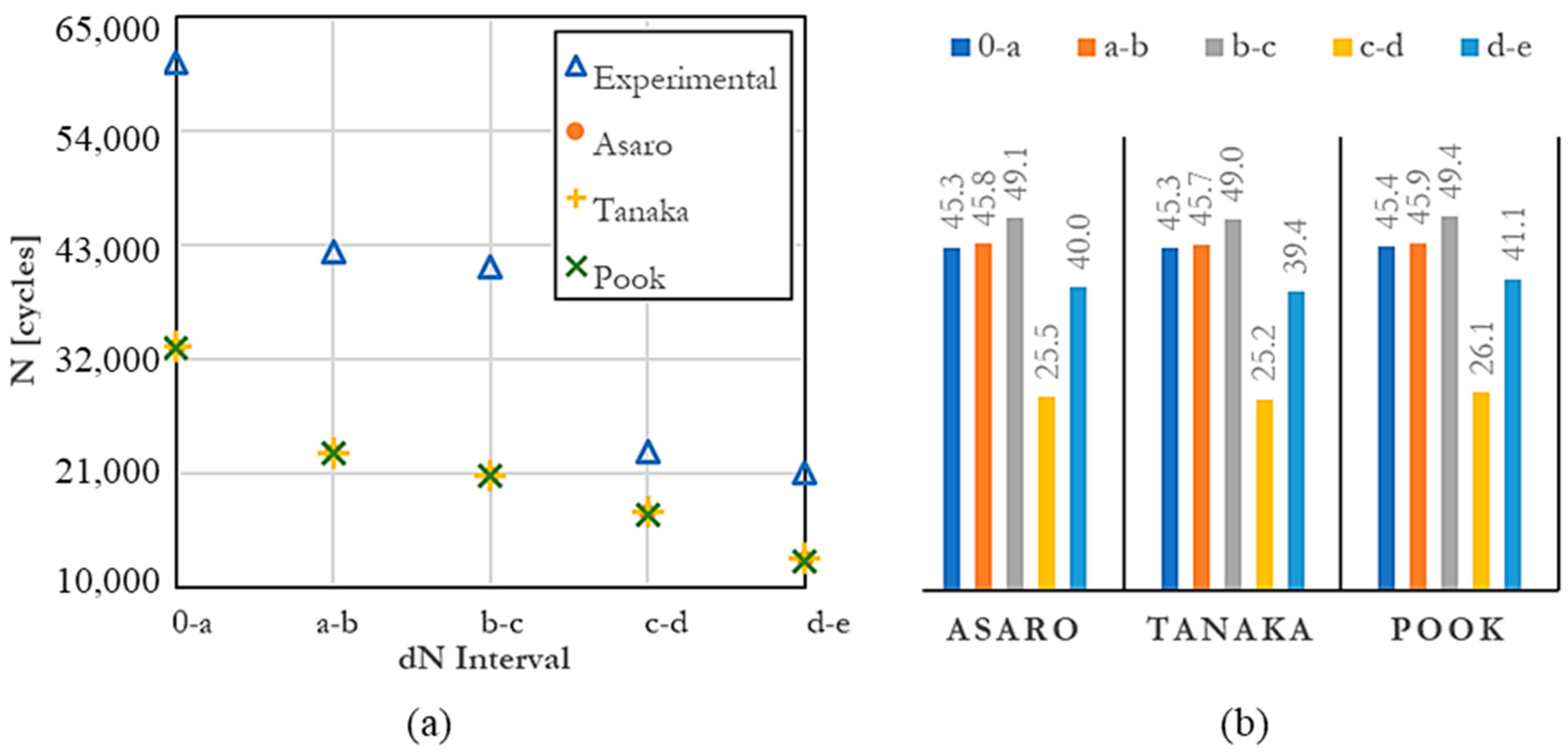
| Point | N [Cycles] | ΔKI | ΔKII | ΔKAsaro | ΔKTanaka | ΔKPook |
|---|---|---|---|---|---|---|
| 0 | 13.12 | 0.46 | 13.13 | 13.12 | 13.14 | |
| a | 17.78 | 0.47 | 17.79 | 17.78 | 17.80 | |
| b | 18.14 | 0.59 | 18.15 | 18.14 | 18.17 | |
| c | 19.67 | 1.17 | 19.70 | 19.67 | 19.77 | |
| d | 22 | 1.55 | 22.05 | 22.00 | 22.16 | |
| e | 26.85 | 3.55 | 27.08 | 26.86 | 27.53 |
| Mixed-Mode Model | C[m/Cycle] | m | R2 |
|---|---|---|---|
| Experimental | 0.9312 | 0.9147 |
Disclaimer/Publisher’s Note: The statements, opinions and data contained in all publications are solely those of the individual author(s) and contributor(s) and not of MDPI and/or the editor(s). MDPI and/or the editor(s) disclaim responsibility for any injury to people or property resulting from any ideas, methods, instructions or products referred to in the content. |
© 2024 by the authors. Licensee MDPI, Basel, Switzerland. This article is an open access article distributed under the terms and conditions of the Creative Commons Attribution (CC BY) license (https://creativecommons.org/licenses/by/4.0/).
Share and Cite
Gómez-Gamboa, E.; Díaz-Rodríguez, J.G.; Mantilla-Villalobos, J.A.; Bohórquez-Becerra, O.R.; Martínez, M.d.J. Experimental and Numerical Evaluation of Equivalent Stress Intensity Factor Models under Mixed-Mode (I+II) Loading. Infrastructures 2024, 9, 45. https://doi.org/10.3390/infrastructures9030045
Gómez-Gamboa E, Díaz-Rodríguez JG, Mantilla-Villalobos JA, Bohórquez-Becerra OR, Martínez MdJ. Experimental and Numerical Evaluation of Equivalent Stress Intensity Factor Models under Mixed-Mode (I+II) Loading. Infrastructures. 2024; 9(3):45. https://doi.org/10.3390/infrastructures9030045
Chicago/Turabian StyleGómez-Gamboa, Estefanía, Jorge Guillermo Díaz-Rodríguez, Jairo Andrés Mantilla-Villalobos, Oscar Rodolfo Bohórquez-Becerra, and Manuel del Jesús Martínez. 2024. "Experimental and Numerical Evaluation of Equivalent Stress Intensity Factor Models under Mixed-Mode (I+II) Loading" Infrastructures 9, no. 3: 45. https://doi.org/10.3390/infrastructures9030045