
Engineering Challenges for Safe and Sustainable Underground Occupation
 , and
, and
Abstract
:1. Introduction
2. Materials and Methods
2.1. Geometry and Soil Parameters
2.2. Finite Element Model and Analyses
- Three- and four-node elements;
- Refined region around cavities, 24 nodes in each tunnel (regions 2 and 3);
- One meter elements on the surface (region 1);
- Lateral regions (4 and 5) 2 m elements on the surface;
- Bottom region (6) 2.5 m elements.
- No excavation and gravitational load to establish the greenfield stresses;
- Excavation of the first tunnel;
- Excavation of the second tunnel.
2.3. Methodology
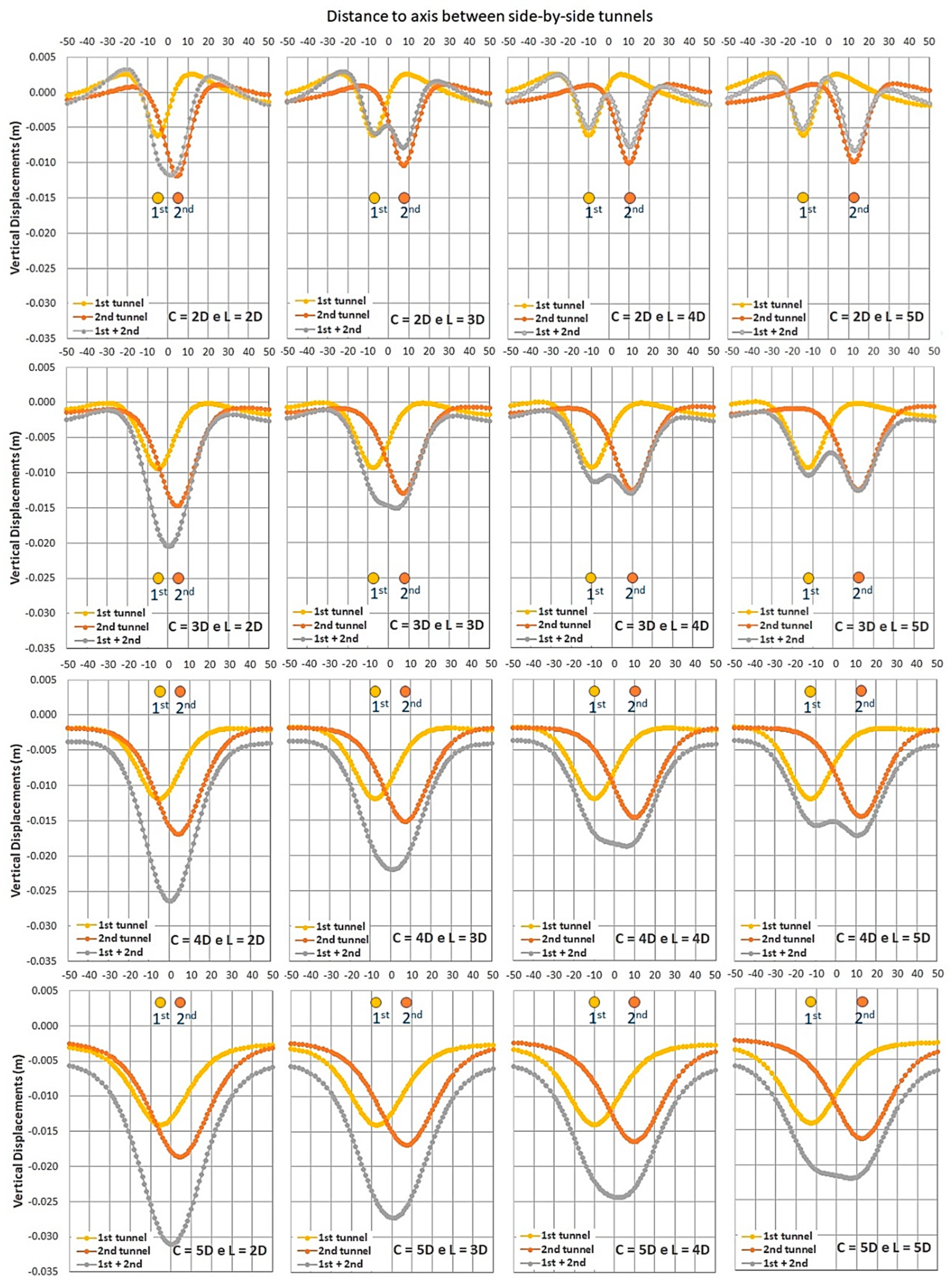
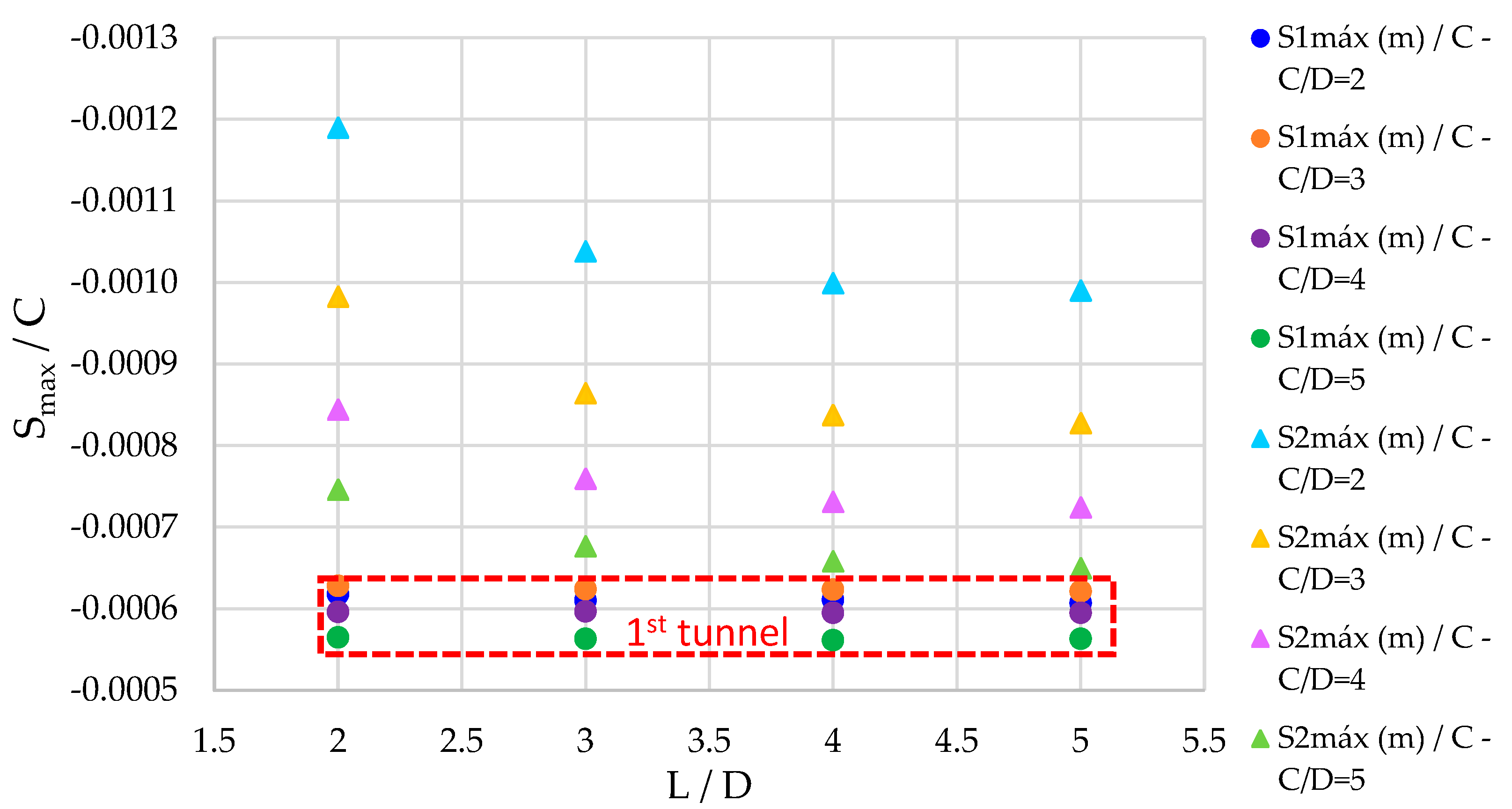
3. Results
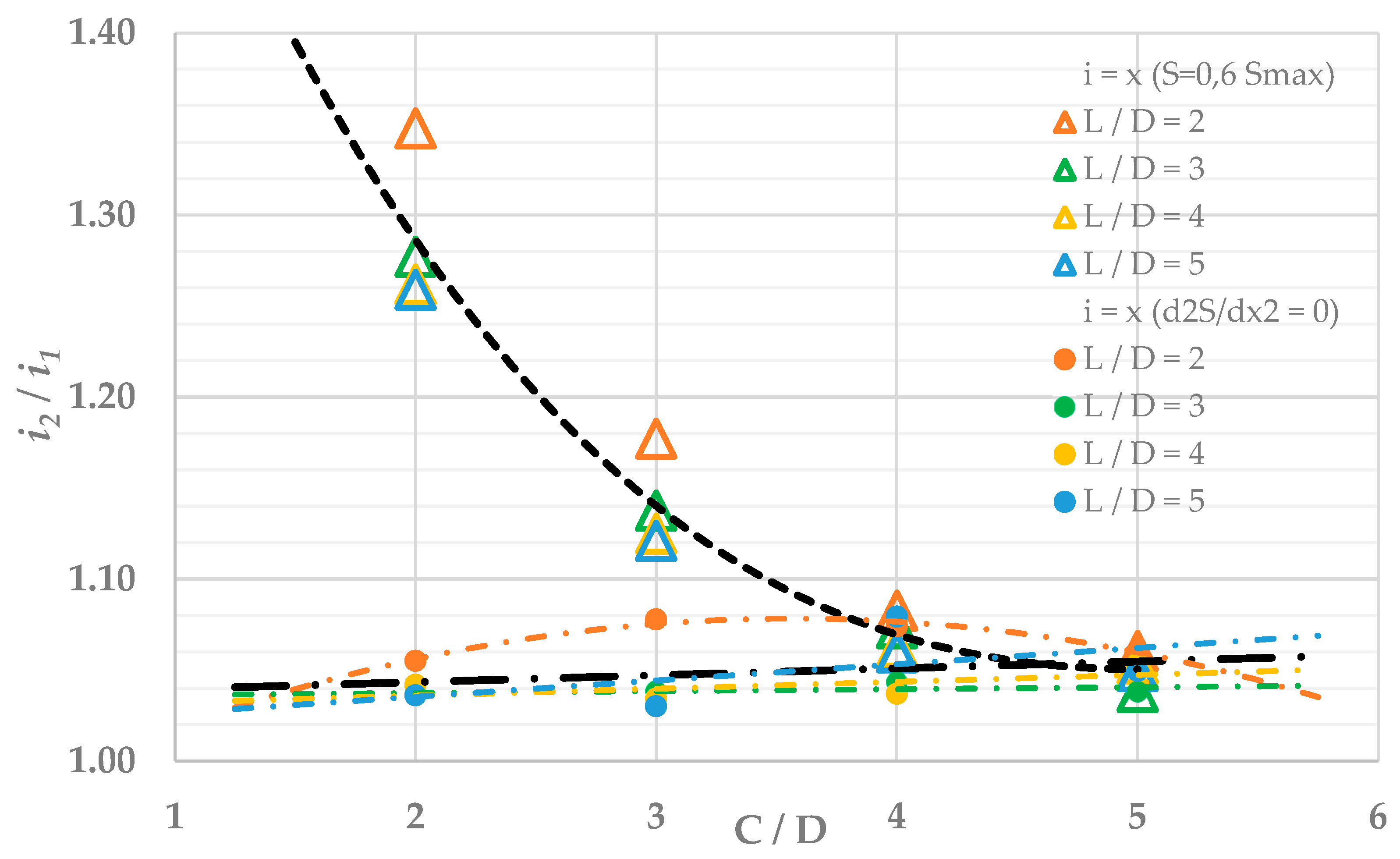
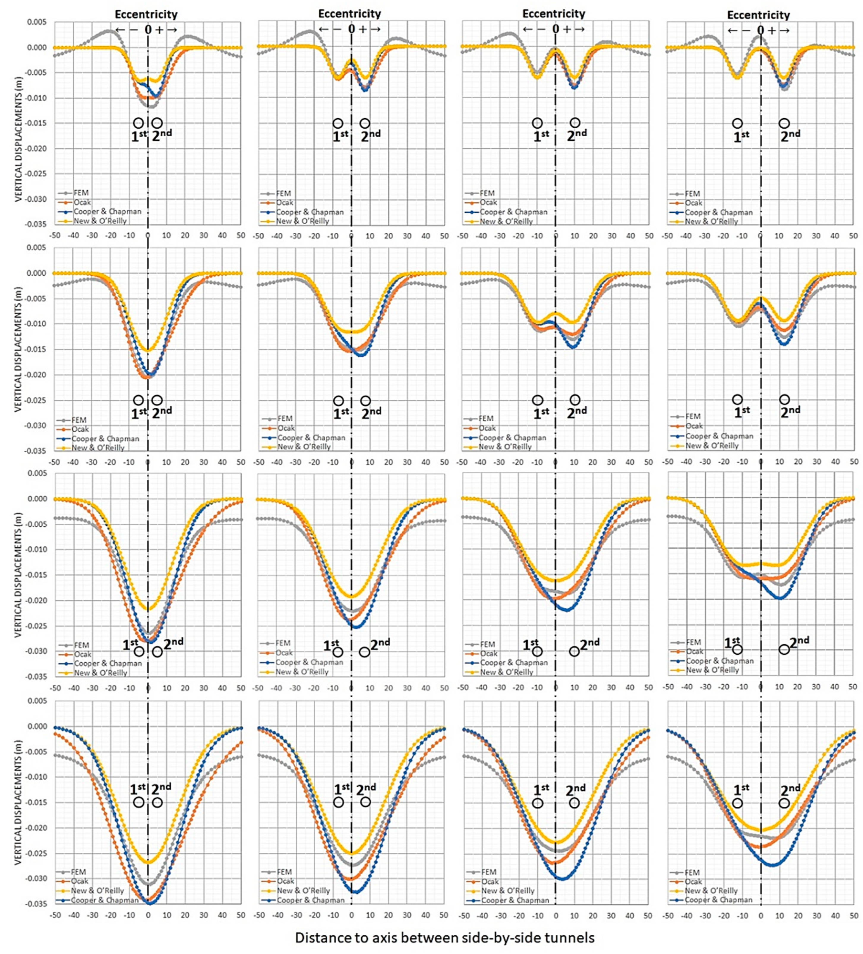
4. Discussion
5. Conclusions
Author Contributions
Funding
Data Availability Statement
Conflicts of Interest
References
- Peck, R.B. Deep excavation and tunneling in soft ground. In Proceedings of the 7th International Conference on Soil Mechanics and Foundation Engineering, Mexico City, Mexico, 1969; Volume 3, pp. 225–290. [Google Scholar]
- Attewell, P.; Farmer, I.; Glossop, N. Ground deformation caused by tunneling in a silty alluvial clay. Ground Eng. 1978, 11, 32–41. [Google Scholar]
- Atkinson, J.H.; Potts, D.M. Subsidence above shallow tunnels in soft ground. J. Geotech. Eng. Div. 1977, 103, 307–325. [Google Scholar] [CrossRef]
- Clough, G.W.; Schmidt, B. Design and Performance of Excavations and Tunnels in Soft Clay. Dev. Geotech. Eng. 1981, 20, 567–634. [Google Scholar]
- O’Reilly, M.P.; New, B.M. Settlements above Tunnels in the United Kingdom—Their Magnitude and Prediction. In Proceedings of the Third International Symposium on Tunneling (Tunnelling ′82), Brighton, UK, 7–11 June 1982; pp. 173–181. [Google Scholar]
- Mair, R.J. Geotechnical aspects of soft ground tunneling. In Proceedings of the International Seminar on Construction Problems in Soft Soils, Sentosa, Singapore, 1–3 December 1983. [Google Scholar]
- Mair, R.J.; Taylor, R.N. Bored tunneling in the urban environment. State-of-the-art Report and Theme Lecture. In Proceedings of the Fourteenth International Conference on Soil Mechanics and Foundation Engineering, Hamburg, Germany, 6–12 September 1997; pp. 2353–2385. [Google Scholar]
- New, B.M.; O’Reilly, M.P. Tunneling induced ground movements; predicting magnitude and effects. In Proceedings of the 4th International Conference on Ground Movements and Structures, Cardiff, UK, 8–11 July 1991; pp. 671–697. [Google Scholar]
- Terzaghi, K. Shield tunnels of the Chicago subway. J. Boston Soc. Civ. Eng. 1942, 29, 163–210. [Google Scholar]
- Moretto, O. Discussion on Deep excavations and tunneling in the soft ground. In Proceedings of the 7th International Conference on Soil Mechanics and Foundation Engineering, Mexico City, Mexico; 1969; Volume 3, pp. 311–315. [Google Scholar]
- Cording, E.J.; Hansmire, W.H. Displacement around soft ground tunnels. In Proceedings of the Pan American Conference Soil Mechanics and Foundation Engineering, Buenos Aires, Argentina, 17–22 November 1975; Volume 4, pp. 571–633. [Google Scholar]
- Akins, K.P.; Abramson, L.W. Tunneling in residual soil and rock. In Proceedings of the Rapid Excavation and Tunneling Conference, Chicago, IL, USA, 12–16 June 1983; Volume 1, pp. 3–24. [Google Scholar]
- Chapman, D.N.; Rogers, C.D.F.; Hunt, D.V.L. Investigating the settlement above closely spaced multiple tunnel constructions in soft ground. In Chapter of the book (Re) Claiming the Underground Space; Publisher Routledge: Amsterdam, The Netherland, 2003; Volume 2, pp. 629–635. [Google Scholar]
- Addenbrooke, T.I.; Potts, D.M. Twin tunnel construction—Ground movements and lining behavior. In Geotechnical Aspects of Underground Construction in Soft Ground; Balkema, A.A., Ed.; Brookfield: Rotterdam, The Netherlands, 1996; ISBN 90 5470 856 8. [Google Scholar]
- Addenbrooke, T.I.; Potts, D.M. Twin tunnel interaction: Surface and Subsurface Effects. Int. J. Geomech. 2001, 1, 249–271. [Google Scholar] [CrossRef]
- Cooper, M.L.; Chapman, D.N.; Rogers, C.D.F.; Chan, A.H.C. Movements in the Piccadilly Line tunnels due to the Heathrow Express construction. Géotechnique 2002, 52, 243–257. [Google Scholar] [CrossRef]
- Ocak, I. A new approach for estimating of settlement curve for twin tunnels. In Proceedings of the World Tunnel Congress, Iguassu Falls, Brazil, 9–15 May 2014. [Google Scholar]
- Qi, X.H.; Zhou, W.H. An efficient probabilistic back-analysis method for braced excavations using wall deflection data at multiple points. Comput. Geotech. 2017, 85, 186–198. [Google Scholar] [CrossRef]
- Zhou, W.; Tan, F.; Yuen, K. Model updating and uncertainty analysis for creep behavior of soft soil. Comput. Geotech. 2018, 100, 135–143. [Google Scholar] [CrossRef]
- Suwansawat, S.; Einstein, H.H. Artificial neural networks for predicting the maximum surface settlement caused by EPB shield tunneling. Tunn. Undergr. Space Technol. 2006, 21, 133–150. [Google Scholar] [CrossRef]
- Chen, R.P.; Zhang, P.; Kang, X.; Zhong, Z.Q.; Liu, Y.; Wu, H.N. Prediction of maximum surface settlement caused by earth pressure balance (EPB) shield tunneling with ANN methods. Soils Found. 2019, 59, 284–295. [Google Scholar] [CrossRef]
- Cheng, Z.L.; Zhou, W.H.; Ding, Z.; Guo, Y.X. Estimation of spatiotemporal response of rooted soil using a machine learning approach. J. Zhejiang Univ. SCIENCE A 2020, 21, 462–477. [Google Scholar] [CrossRef]
- Cheng, Z.L.; Zhou, W.H.; Garg, A. The genetic programming model for estimating soil suction in shallow soil layers in the vicinity of a tree. Eng. Geol. 2020, 268, 105506. [Google Scholar] [CrossRef]
- Gao, Y.; Liu, Y.; Tang, P.; Mi, C. Modification of Peck Formula to Predict Surface Settlement of Tunnel Construction in Water-Rich Sandy Cobble Strata and Its Program Implementation. Sustainability 2022, 14, 14545. [Google Scholar] [CrossRef]
- Zhao, W.; Jia, P.J.; Zhu, L. Analysis of the Additional Stress and Ground Settlement Induced by the Construction of Double-O-Tube Shield Tunnels in Sandy Soils. Appl. Sci. 2019, 9, 1399. [Google Scholar] [CrossRef] [Green Version]


| Author | i Value |
|---|---|
| Peck [1] | where n = 0.8 to 1.0 |
| Attewell et al. [2] | where α = 1 and n = 1.0 |
| Atkinson and Potts [3] | i = 0.25 (Zo + R) loose sand i = 0.25 (1.5Zo + 0.5R) dense sand/over consolidated clay |
| Clough and Schmidt [4] | where α = 1 and n = 0.8 |
| O’Reilly and New [5] | cohesive soil granular soil |
| Mair [6] | |
| Mair and Taylor [7] | Kclays = 0.4 a 0.5 and Ksand = 0.25 a 0.45 |
| Soil Type | Clay |
|---|---|
| Constitutive model | Isotropic linear elastic |
| Young’s module | 20 MPa (constant) |
| Poisson | 0.35 |
| Specific weight | 16.5 kN/m³ |
| Geometric Configuration | 1st Tunnel Trough | 2nd Tunnel Trough | |||
|---|---|---|---|---|---|
| L (1)/D | C (2)/D | S1max (m) | S1max/C | S2max (m) | S2max/C |
| 2 | 2 | −0.00618 | −0.0006 | −0.01190 | −0.0012 |
| 2 | 3 | −0.00610 | −0.0006 | −0.01038 | −0.0010 |
| 2 | 4 | −0.00611 | −0.0006 | −0.00999 | −0.0008 |
| 2 | 5 | −0.00607 | −0.0006 | −0.00990 | −0.0007 |
| 3 | 2 | −0.00942 | −0.0006 | −0.01474 | −0.0010 |
| 3 | 3 | −0.00936 | −0.0006 | −0.01296 | −0.0009 |
| 3 | 4 | −0.00935 | −0.0006 | −0.01256 | −0.0008 |
| 3 | 5 | −0.00932 | −0.0006 | −0.01241 | −0.0007 |
| 4 | 2 | −0.01192 | −0.0006 | −0.01688 | −0.0010 |
| 4 | 3 | −0.01193 | −0.0006 | −0.01519 | −0.0008 |
| 4 | 4 | −0.01190 | −0.0006 | −0.01462 | −0.0007 |
| 4 | 5 | −0.01190 | −0.0006 | −0.01448 | −0.0007 |
| 5 | 2 | −0.01412 | −0.0006 | −0.01865 | −0.0010 |
| 5 | 3 | −0.01408 | −0.0006 | −0.01691 | −0.0008 |
| 5 | 4 | −0.01403 | −0.0006 | −0.01645 | −0.0007 |
| 5 | 5 | −0.01408 | −0.0006 | −0.01624 | −0.0006 |
| Geometric Configuration | FEM i = x (d2S/dx2 = 0) (3) | FEM i = x (S = 0.606Smax) | |||||
|---|---|---|---|---|---|---|---|
| C (2)/D | L (1)/D | i1 (m) | i2/i1 | i2 (m) | i1 (m) | i2/i1 | i2 (m) |
| 2 | 2 | 5.26 | 1.06 | 5.55 | 4.26 | 1.35 | 5.74 |
| 2 | 3 | 5.24 | 1.04 | 5.43 | 4.26 | 1.28 | 5.44 |
| 2 | 4 | 5.25 | 1.04 | 5.47 | 4.24 | 1.26 | 5.35 |
| 2 | 5 | 5.25 | 1.04 | 5.44 | 4.25 | 1.26 | 5.35 |
| 3 | 2 | 7.32 | 1.08 | 7.89 | 7.62 | 1.18 | 8.97 |
| 3 | 3 | 7.31 | 1.04 | 7.59 | 7.63 | 1.14 | 8.68 |
| 3 | 4 | 7.31 | 1.03 | 7.56 | 7.60 | 1.13 | 8.55 |
| 3 | 5 | 7.29 | 1.03 | 7.51 | 7.60 | 1.12 | 8.52 |
| 4 | 2 | 9.45 | 1.07 | 10.15 | 11.37 | 1.08 | 12.31 |
| 4 | 3 | 9.44 | 1.04 | 9.85 | 11.37 | 1.07 | 12.20 |
| 4 | 4 | 9.45 | 1.04 | 9.80 | 11.38 | 1.06 | 12.09 |
| 4 | 5 | 9.32 | 1.08 | 10.06 | 11.38 | 1.06 | 12.06 |
| 5 | 2 | 11.72 | 1.06 | 12.43 | 15.39 | 1.02 | 15.75 |
| 5 | 3 | 11.80 | 1.04 | 12.25 | 15.41 | 1.03 | 15.84 |
| 5 | 4 | 11.75 | 1.05 | 12.38 | 15.44 | 1.03 | 15.84 |
| 5 | 5 | 11.11 | 1.05 | 11.66 | 15.45 | 1.02 | 15.81 |
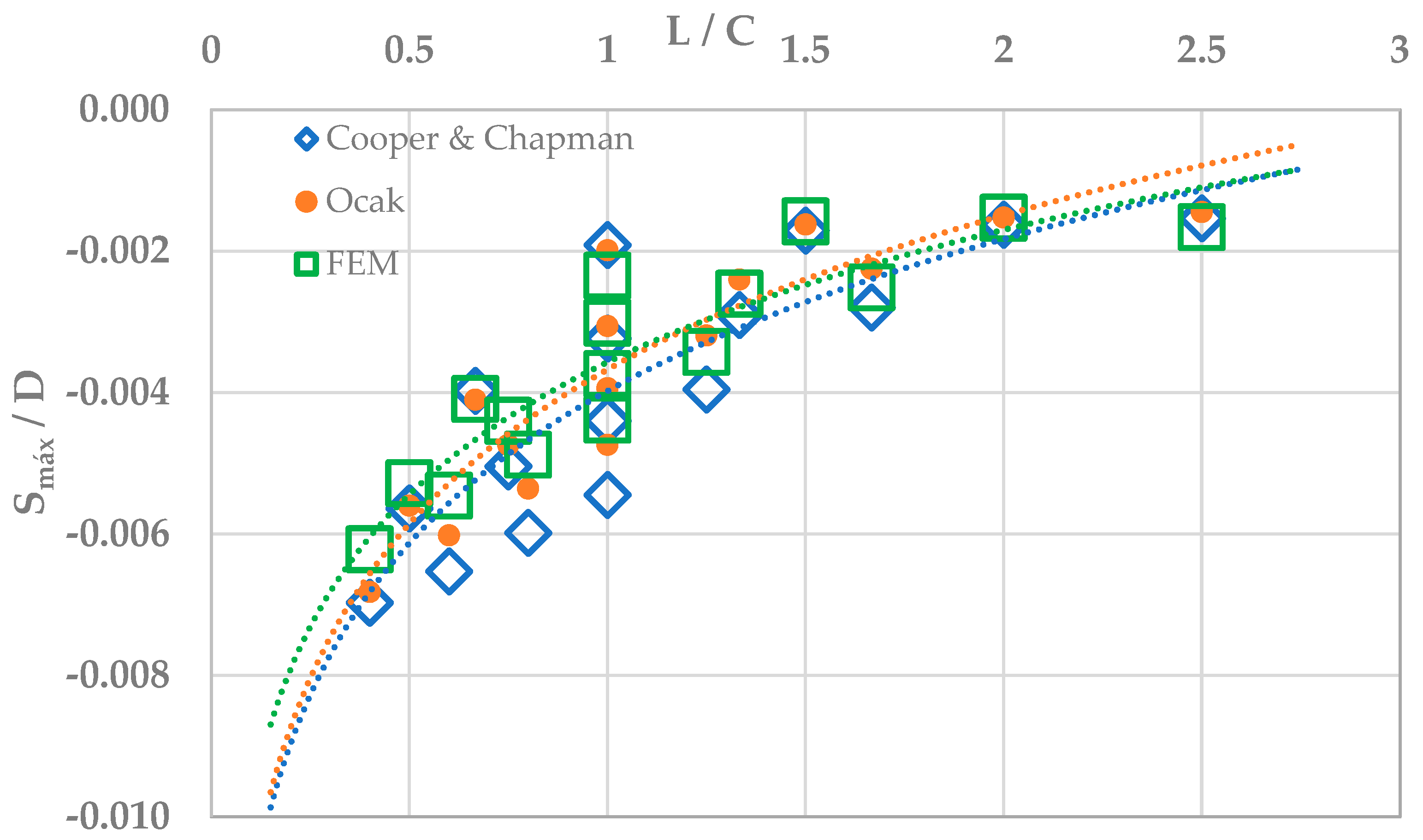
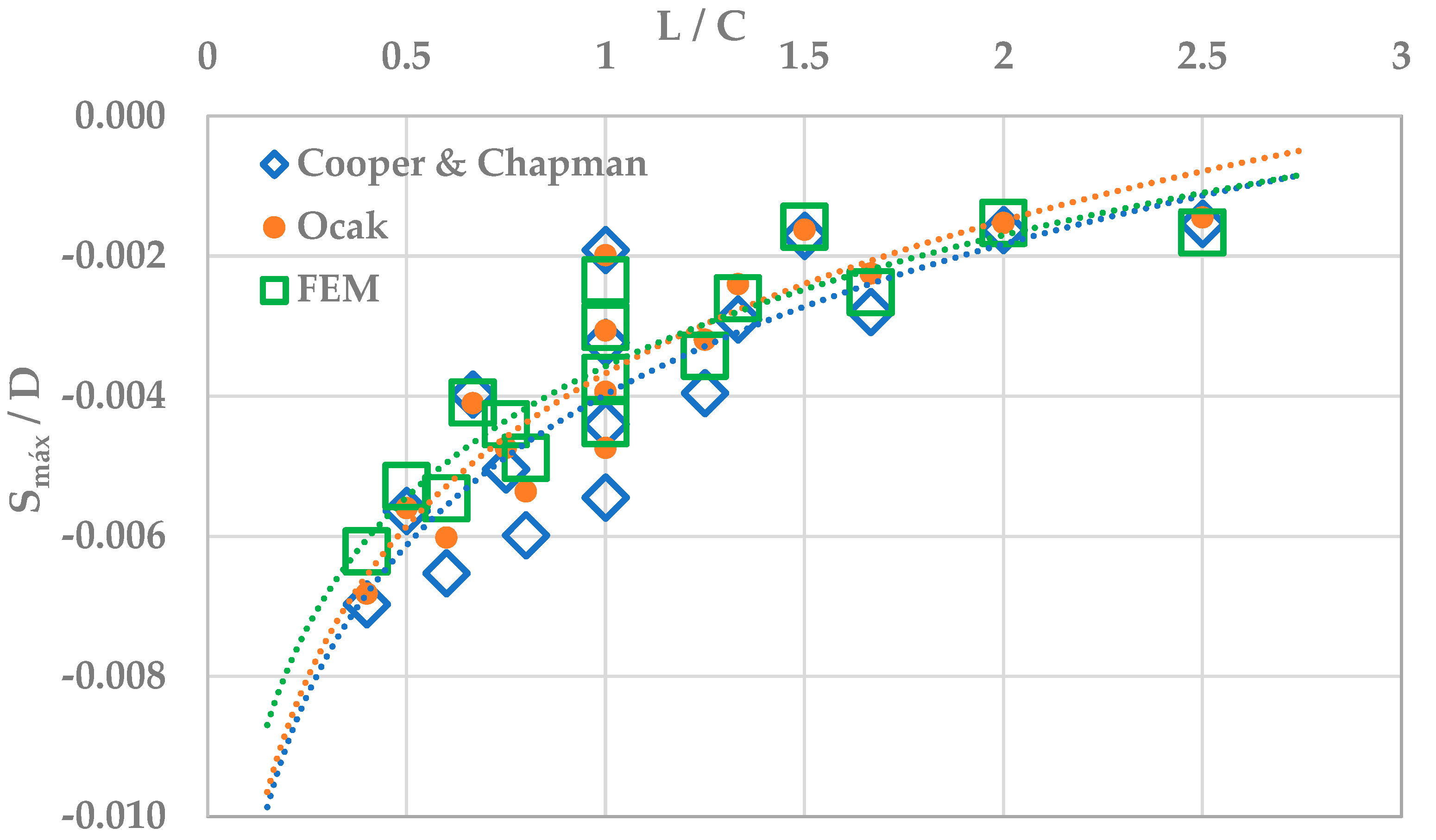
| Geometric Configuration | Smáx (m) | Eccentricity (3) (m) | |||||
|---|---|---|---|---|---|---|---|
| C (2)/D | L (1)/D | Cooper and Chapman | Ocak | FEM | Cooper and Chapman | Ocak | FEM |
| 2 | 2 | −0.0096 | −0.0099 | −0.0117 | 4.0 | 2.0 | 2.0 |
| 2 | 3 | −0.0199 | −0.0205 | −0.0205 | 2.0 | −1.0 | 3.0 |
| 2 | 4 | −0.0282 | −0.0280 | −0.0264 | 1.0 | −1.0 | 0.0 |
| 2 | 5 | −0.0349 | −0.0341 | −0.0311 | 1.0 | −1.0 | 0.0 |
| 3 | 2 | −0.0086 | −0.0081 | −0.0079 | 7.0 | 7.0 | 7.0 |
| 3 | 3 | −0.0162 | −0.0153 | −0.0151 | 5.0 | −1.0 | 4.0 |
| 3 | 4 | −0.0252 | −0.0237 | −0.0220 | 3.0 | −1.0 | 1.0 |
| 3 | 5 | −0.0326 | −0.0301 | −0.0273 | 3.0 | −1.0 | 1.0 |
| 4 | 2 | −0.0081 | −0.0076 | −0.0076 | 10.0 | 10.0 | 10.0 |
| 4 | 3 | −0.0145 | −0.0120 | −0.0130 | 9.0 | 9.0 | 9.0 |
| 4 | 4 | −0.0220 | −0.0197 | −0.0187 | 6.0 | −2.0 | 6.0 |
| 4 | 5 | −0.0299 | −0.0268 | −0.0244 | 4.0 | −2.0 | 2.0 |
| 5 | 2 | −0.0077 | −0.0073 | −0.0083 | 12.0 | 12.0 | 13.0 |
| 5 | 3 | −0.0140 | −0.0113 | −0.0126 | 12.0 | 12.0 | 13.0 |
| 5 | 4 | −0.0198 | −0.0160 | −0.0171 | 10.0 | 6.0 | 11.0 |
| 5 | 5 | −0.0272 | −0.0237 | −0.0219 | 6.0 | −1.0 | 7.0 |
| Geometric Configuration | Cooper and Chapman | Ocak | FEM (3) | |||||||
|---|---|---|---|---|---|---|---|---|---|---|
| C (2)/D | L (1)/D | i1 (m) | i2/i1 | (3)i2 (m) | i1 (m) | i2/i1 | i2 (m) | i1 (m) | i2/i1 | i2 (m) |
| 2 | 2 | 4.26 | 1.00 | 4.25 | 4.26 | 1.35 | 5.74 | 5.26 | 1.06 | 5.55 |
| 2 | 3 | 4.26 | 1.00 | 4.25 | 4.26 | 1.28 | 5.44 | 5.24 | 1.04 | 5.43 |
| 2 | 4 | 4.24 | 1.12 | 4.75 | 4.24 | 1.26 | 5.35 | 5.25 | 1.04 | 5.47 |
| 2 | 5 | 4.25 | 1.00 | 4.25 | 4.25 | 1.26 | 5.35 | 5.25 | 1.04 | 5.44 |
| 3 | 2 | 7.62 | 0.98 | 7.50 | 7.62 | 1.18 | 8.97 | 7.32 | 1.08 | 7.89 |
| 3 | 3 | 7.63 | 0.98 | 7.50 | 7.63 | 1.14 | 8.68 | 7.31 | 1.04 | 7.59 |
| 3 | 4 | 7.60 | 0.99 | 7.50 | 7.60 | 1.12 | 8.55 | 7.31 | 1.03 | 7.56 |
| 3 | 5 | 7.60 | 0.99 | 7.50 | 7.60 | 1.12 | 8.52 | 7.29 | 1.03 | 7.51 |
| 4 | 2 | 11.37 | 1.01 | 11.50 | 11.37 | 1.08 | 12.31 | 9.45 | 1.07 | 10.15 |
| 4 | 3 | 11.37 | 1.01 | 11.50 | 11.37 | 1.07 | 12.20 | 9.44 | 1.04 | 9.85 |
| 4 | 4 | 11.38 | 1.01 | 11.50 | 11.38 | 1.06 | 12.09 | 9.45 | 1.04 | 9.80 |
| 4 | 5 | 11.38 | 1.01 | 11.50 | 11.38 | 1.06 | 12.06 | 9.32 | 1.08 | 10.06 |
| 5 | 2 | 15.39 | 1.01 | 15.50 | 15.39 | 1.02 | 15.75 | 11.72 | 1.06 | 12.43 |
| 5 | 3 | 15.41 | 1.01 | 15.50 | 15.41 | 1.03 | 15.84 | 11.80 | 1.04 | 12.25 |
| 5 | 4 | 15.44 | 1.00 | 15.50 | 15.44 | 1.03 | 15.84 | 11.75 | 1.05 | 12.38 |
| 5 | 5 | 15.45 | 1.00 | 15.50 | 15.45 | 1.02 | 15.81 | 11.11 | 1.05 | 11.66 |
Disclaimer/Publisher’s Note: The statements, opinions and data contained in all publications are solely those of the individual author(s) and contributor(s) and not of MDPI and/or the editor(s). MDPI and/or the editor(s) disclaim responsibility for any injury to people or property resulting from any ideas, methods, instructions or products referred to in the content. |
© 2023 by the authors. Licensee MDPI, Basel, Switzerland. This article is an open access article distributed under the terms and conditions of the Creative Commons Attribution (CC BY) license (https://creativecommons.org/licenses/by/4.0/).
Share and Cite
Cavalcanti, M.d.C.R.; Nahas Ribeiro, W.; Cabral dos Santos Junior, M. Engineering Challenges for Safe and Sustainable Underground Occupation. Infrastructures 2023, 8, 42. https://doi.org/10.3390/infrastructures8030042
Cavalcanti MdCR, Nahas Ribeiro W, Cabral dos Santos Junior M. Engineering Challenges for Safe and Sustainable Underground Occupation. Infrastructures. 2023; 8(3):42. https://doi.org/10.3390/infrastructures8030042
Chicago/Turabian StyleCavalcanti, Maria do Carmo Reis, Wagner Nahas Ribeiro, and Marcelo Cabral dos Santos Junior. 2023. "Engineering Challenges for Safe and Sustainable Underground Occupation" Infrastructures 8, no. 3: 42. https://doi.org/10.3390/infrastructures8030042