Sensor Data Quality in Ships: A Time Series Forecasting Approach to Compensate for Missing Data and Drift in Measurements of Speed through Water Sensors

Abstract

In this paper, four machine learning algorithms are examined regarding their effectiveness in dealing with a complete lack of sensor drift values for a crucial parameter for ship performance evaluation, such as a ship’s speed through water (STW). A basic Linear Regression algorithm, a more sophisticated ensemble model (Random Forest) and two modern Recurrent Neural Networks i.e., Long Short-Term Memory (LSTM) and Neural Basis Expansion Analysis for Time Series (N-Beats) are evaluated. A computational algorithm written in python language with the use of the Darts library was developed for this scope. The results regarding the selected parameter (STW) are provided on a real- or near-to-real-time basis. The algorithms were able to estimate the speed through water in a progressive manner, with no initial values needed, making it possible to replace the complete missingness of the label data. A physical model developed with the simulation platform of Siemens Simcenter Amesim is used to calculate the ship STW under the real operating conditions of a banker ship type during a period of six months. These theoretically obtained values are used as reference values (“ground-truth” values) to evaluate the performance of each of the four machine learning algorithms examined.

1. Introduction

It is common knowledge that the cost of energy is most likely to rise in the years to come. Recent events such as the war in Ukraine have made clear that the cost of energy is a highly complex and flexible aspect dictated by economic and geopolitical criteria that cannot be estimated with precision [1]. In the shipping industry, the cost of fuel has become the dominant factor in the operational costs of ships; therefore, all shipping companies are starting to adopt new technologies in order to reduce their operating expenses and become more competitive [2]. This is also dictated by the international regulations regarding CO₂ emissions (the Carbon Intensity Indicator (CII) and the Energy Efficiency eXisting Ship Index (EEXI)).

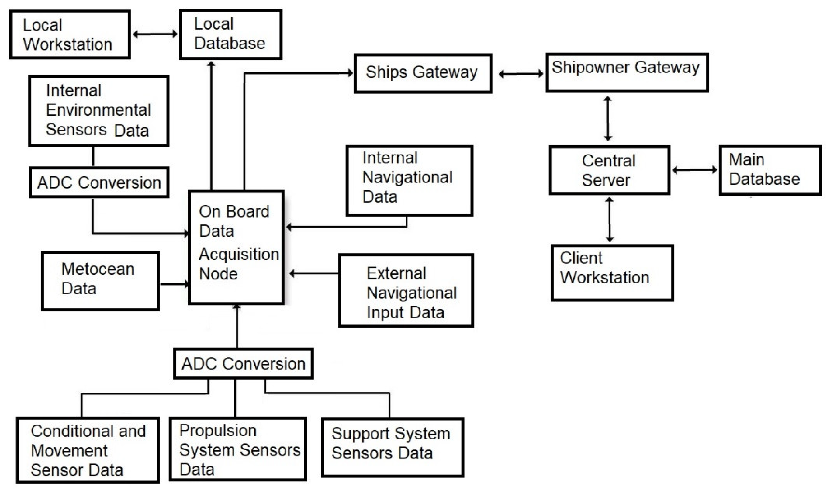
A key strategy of shipping companies to compensate for the aforementioned variable economic environment is the adoption of modern systems that are based on IoT technologies and help to operate ships in a more efficient way [3]. State-of-the-art systems based on Industry 4.0 technologies are currently being installed on board ships. These systems collect data from various sensors, and process and store these data, to give insights to the crew, the shipping company personnel and the operators about the operating conditions of each ship and how they affect the ship’s performance and efficiency.

The “quality” of the data, in terms of consistency and accuracy, that are collected with these systems is probably the most important aspect of their overall performance. Missing or inaccurate data can lead to biased estimations or even the incapability to monitor performance. In the case of ships, this problem becomes more crucial when taking into account that while sailing, the resources (if any) to identify and repair sensors/data acquisition systems are limited.

Dealing with random missing data in log files is a common problem/challenge in all modern data acquisition, control and presentation systems (ADLMs) that are installed, but dealing with the complete missingness of a crucial sensor or compensating for sensor drift is a much more difficult and complex problem. The most common methods for data imputation that are usually implemented are the following [4]:

• Use of the next or previous value.
• Unsupervised machine learning (ML) techniques such as K-Nearest Neighbors.
• Use of the maximum, minimum, mean, moving average or median value.
• Average or linear interpolation.
• Use of a fixed value.

Unfortunately, all the above methods are not adequate to be used when we are missing a very large number of continuous data (a series of data) or when we cannot validate the accuracy of readings in order to calibrate the method used. In order to compensate for this problem, it has been proposed to use a type of Missing Value Prediction technique. A number of papers published recently deal with the sensor drift problem. In [5], an LSTM and SVM Multi-Class Ensemble Learning model was used to deal with the drift of a gas sensor that improved the accuracy of the sensor over a 3-year period. Numerous algorithms have been proposed in the literature that are able to detect unreliable/drifted sensor data in a sensor network [6]. In [7], machine learning approaches to address IoT sensor drift are presented that need low computational power and, thus, can be implemented in any IoT sensor network. Time series forecasting algorithms are used to compensate for either the complete missingness of sensor data or sensor drift. Supervised ML used in time series forecasting is a very promising approach in order to deal with the missingness of a large amount of data. The missing data can be set as the label (dependent value), and all the other data can be set as attributes (independent data) in order to fill in the missing data. In general, all ML models learn with respect to the distribution of the features in the training data. If the feature space distribution of the data changes, there will be a mismatch between the model’s representation and the actual data, resulting in decreased performance. This inherent characteristic of ML models is used in the present study to detect and compensate for sensor drift.

The aim of this study is to examine the possibility to address and solve the aforementioned problem with the use of machine learning or deep learning techniques. We evaluate whether it is possible to compensate for sensor drift if we train an ML model to predict a sensor value when a sensor is new and in good condition and then transfer the model’s “knowledge” to actual conditions. Time series forecasting algorithms are used to compensate for either the complete missingness of sensor data or sensor drift. Supervised ML used in time series forecasting is a very promising approach in order to deal with the missingness of a large amount of data. The missing data can be set as the label (dependent value), and all the other data can be set as attributes (independent data) in order to fill in the missing data. In general, all ML models learn with respect to the distribution of the features in the training data. If the feature space distribution of the data changes, there will be a mismatch between the model’s representation and the actual data, resulting in decreased performance. This inherent characteristic of ML models is used in the present study to detect and compensate for sensor drift. 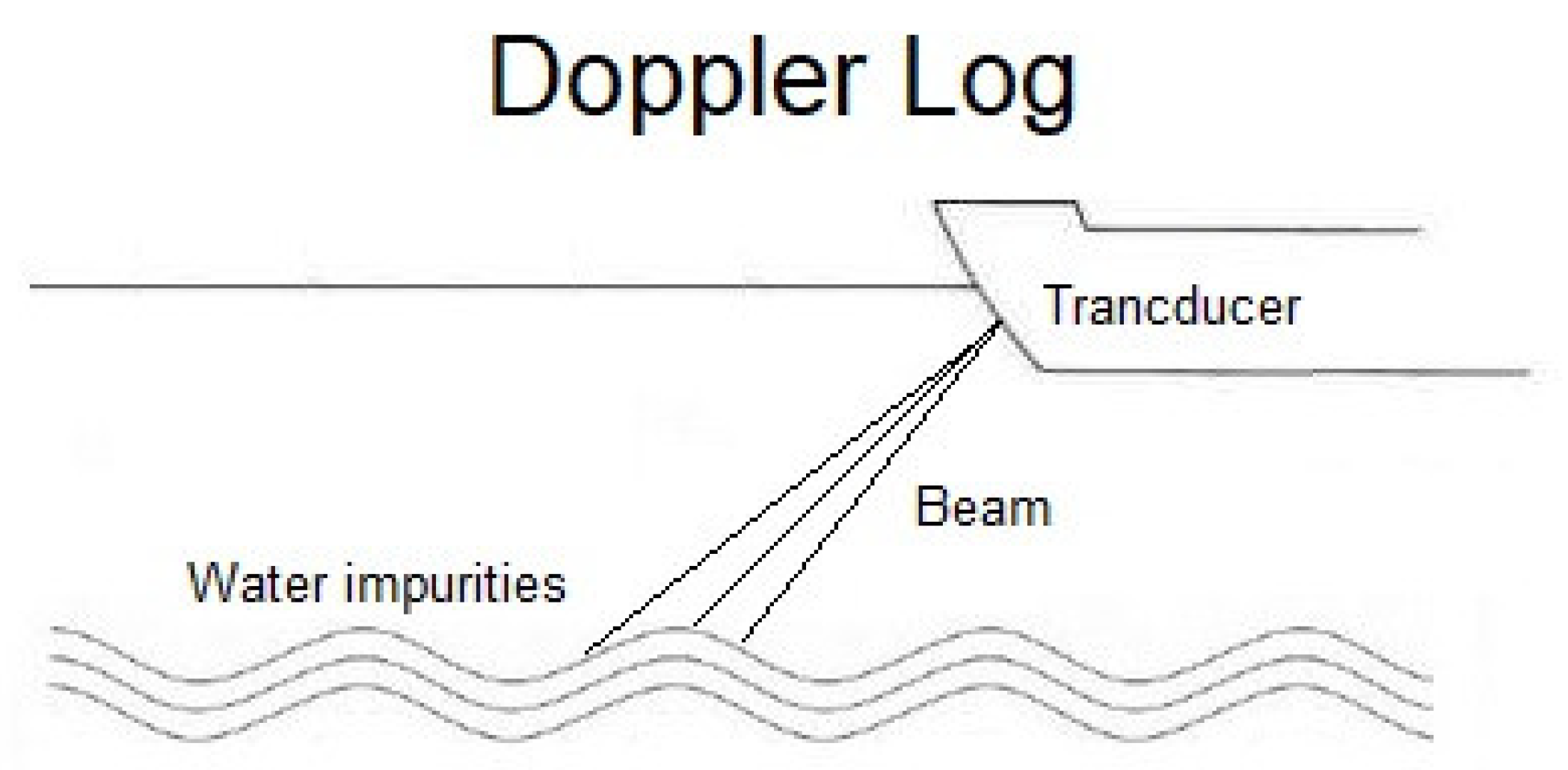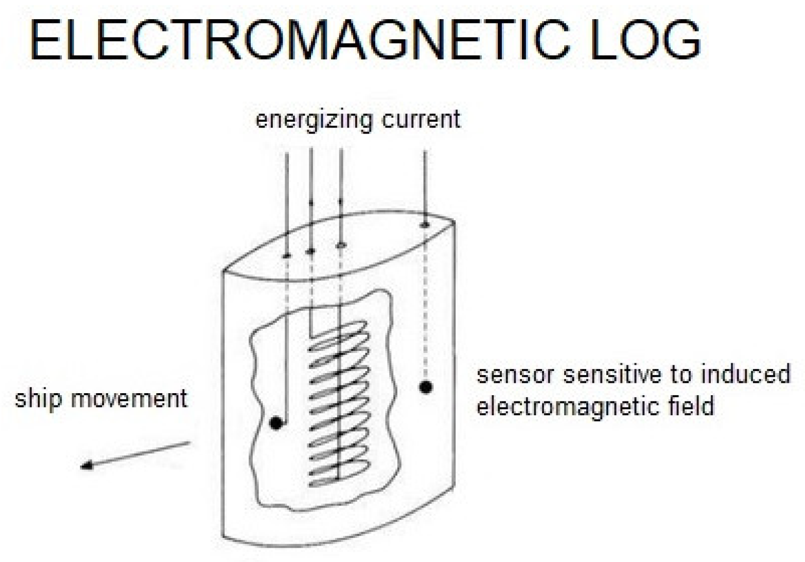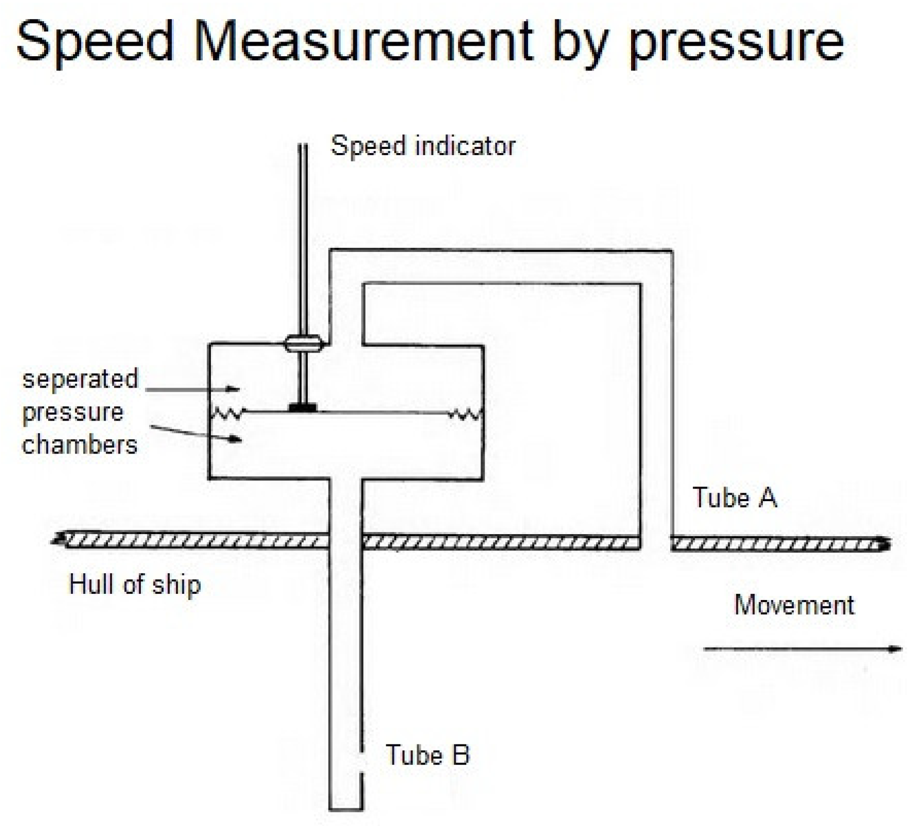The paper content is organized as follows: In Section 2, the importance of the sea though water (STW) value in ship performance prediction is described. The different types of STW sensors that are installed in the majority of ships are presented. Their working principle is explained to support their high exposure to the possibility of drifting in their accuracy. The basic configuration of modern ADLM systems and the mechanisms of missing values are presented in Section 3. Section 4 is dedicated to the analysis of the proposed method. In Section 5, the results of this study are presented, and in Section 6, we conclude by briefly discussing the results and providing future perspectives/challenges.

2. The Significance of Speed through Water

There are two different values that describe a ship’s speed while cruising: the speed over ground (SOG), which is the speed of the ship relative to the surface of the Earth, and the speed through water (STW), which is the speed of the ship relative to the water surrounding it. The SOG is needed to calculate the time needed for a ship to cover a certain distance, but it is the STW that is, probably, the most important factor that affects a ship’s performance. The energy that is needed for the propulsion system is by far the largest energy “consumer” in ships. Depending on the ship type, the percentage of a ship’s propulsion power demand can be as high as 70% of the total energy consumption when it is sailing at cruising speed [8]. This amount of energy compensates mainly for the energy losses due to the ship movement relative to the water (hydrodynamic resistance) being directly related to the STW. The accurate measurement or estimation of STW is a key parameter for numerous crucial applications related to ship design, operation and performance optimization [9].

2.1. Types of STW Measurement

There are mainly three techniques that have been established over the years as the industrial standard for the measurement of STW. Each of them makes use of different physical phenomena that are related to or affected by the movement of a ship in water. The first of them relies on the Doppler effect. A transducer (Doppler log) transmits ultrasound pulses and measures the backscatter echo from any impurity that lies in the water [10,11]. The frequency shift (Doppler shift) is then used to calculate the ship’s STW. In Figure 1, a schematic representation of the Doppler speed log is presented.

The electromagnetic speed log (EM log) working principle is based on the induction law. If any conductor moves across a magnetic field, an electromotive force (EMF) is set up in the conductor. The induced EMF is directly proportional to the velocity of movement. An EM log consists of two electrodes in a common shell that are placed beneath the hull. The current induced in these electrodes by the seawater flowing past is a function of speed. As the vessel moves, the seawater (conductor) relatively moving through the magnetic field induces a small electromagnetic field. This induced EMF is detected, amplified and measured with two sensors on the hull region. To convert the sensor measurements to the STW, proper calibration is needed [12].

The induced EMF is given using Equation (1):

EMF = F × L × V,

(1)

where F = the magnetic field, L = the length of the conductor and V = the velocity of the conductor’s movement through the magnetic field. Figure 2 shows the main parts of an EM log probe.

The last, older and, at present, not so widespread STW measurement technique relies on pressure variation. When a tube with an opening is submerged in water, a pressure (static) related to the depth of the opening is developed. If the tube starts to move through the water, a second pressure called dynamic pressure is then added. The total pressure in the tube (called a pitot tube) is, therefore, the sum of both the static and dynamic pressures. Having a way to eliminate the static pressure and measure only the one that is induced by the relative velocity of the tube (the dynamic pressure) gives us the ability to calculate the movement speed [12]. The elimination of the static pressure is accomplished by using a second tube (with a direction tangential to the water velocity vector) and two pressure chambers, as presented in Figure 3.

2.2. Drifting of Sensor Readings

Having established an understanding of the working principles of the three main technologies for STW measurement, it is easy to identify possible causes that can lead to the gradually reduced accuracy of readings (drift). Considering that a ship’s STW is related to the propulsion power to the power of three, even the slightest inaccuracy in the STW measurement can lead to remarkable errors in the estimated ship performance. Despite the indisputable importance of the accurate measurement of STW and the existence of speed log sensors in the majority of ships, several recent studies have highlighted the fact that a speed log is one of the most inaccurate measurement devices onboard [10,13,14]. As an example, a recent study on the accuracy of these sensors revealed that in most cases, the best accuracy of EM logs is around 0.3 knots, while there are often cases in which the deviations are higher than 1 knot [15].

The main reason for this paradox is the fact that in modern shipping, speed over ground (SOG) measured via global positioning system (GPS) is the preferred method for speed measurements by crews due to its accuracy and ease of use, which, in many cases, leads to a lack of thorough maintenance of the speed log devices that are installed onboard. Additionally, there are some inherent characteristics of STW sensors themselves that affect the accuracy of their readings. In the case of a Doppler log, the “window” of the transducer where a beam is transmitted and received can be partially or completely blocked by marine growth. This leads to false (biased) readings. To make things worse, marine growth is a long and slow process that is affected by the intervals during which the ship is stationary along with the environmental conditions (water salinity and temperature). It is then nearly impossible to accurately calculate the sensor drift due to marine fouling in order to compensate for it with proper calibration. Marine growth can also affect an EM log by disrupting the hydrodynamic form of the EM log probe and thus altering the flow of water around it. This leads to biased readings of STW with this kind of sensor. In extreme cases, marine growth can even affect sensors that use pressure by narrowing or even blocking the openings of the tubes that these sensors use.

The second cause of sensor drift is a lack of calibration. All of the above sensors need frequent calibration to ensure their smooth operation and the validity of their measurements. The calibration procedure requires traveling some distances with the ship to different headings and with controlled conditions. This can cause a major problem since, on one hand, it is very difficult to identify the drift, and on the other hand, even if the crew manages to identify it, in-service recalibration will be required. There are, however, no easy ways of recalibrating speed logs for a ship that is in service [16].

3. The Problem of Missing Values

Missing data logs is a very common problem that occurs in a ship’s onboard automatic acquisition, recording and transmitting systems. Multiple types of malfunctions can lead to this result [17]. In order to be able to monitor the performance of a ship in a consistent and accurate manner, the missing data logs must not exceed a certain amount. A great deal of missing or inaccurate data logs can render the process of ship performance monitoring inaccurate or, in extreme cases, impossible. The fact that a ship’s crew often lacks the ability to investigate and/or repair the cause of missing values, combined with the fact that ships are usually beyond reach, can lead to the loss of an entire trip’s worth of data.

3.1. Configurations of Onboard Log Systems

In recent years and with the rise of the fourth industrial revolution, all new ship buildings, and an increasing number of existing ones, adopt some kind of central control and monitoring system [18]. The main purpose of these systems is to make it possible to safely operate a complex system (such as a synchronous ship) with a reduced number of crew members. These systems automatically take the measurements, log the data and record the parameters needed to fill the numerous reports crew members are obligated to fill. Moreover, it is possible that all or part of these data are transmitted to the operator and shipowners in order to assist them in maximizing ship performance, help the crew with troubleshooting and plan the maintenance schedule.

In synchronous ships, Automated Data Logging and Monitoring (ADLM) systems are able to collect the information from the ships’ onboard sensors and other connected peripherals. A basic block diagram of such a modern system is presented in Figure 4.

Modern ADLM systems are very complicated. Multiple inputs with different formats have to be combined in order to analyze, process and store the information [19]. As an example, one can follow the “path” of a pressure sensor installed in a tank on board a ship. First, there is the sensor itself that transforms the pressure into an electric signal (usually in the form of a current in the range of 4 to 20 mA). This current then has to be transferred to an ADC converter that will transform it into a digital signal that is ready to be processed. Different transfer protocols and interfaces such as Ethernet, Modbus, AS-I bus, Matter, Zigbee, MQTT and NMEA may be used to combine and transfer the digital information to the onboard data acquisition nodes. [20]. Next in line is the conversion of all the sensor data to a selected “master” frequency. This frequency will form the intervals of the different data instances. These instances occupy a local database and are analyzed, presented and transferred to the central server [21,22].

Such a complex system of integration that works in the harsh environment of a ship has a very high probability of missing data occurrence. Data can be lost or misinterpreted due to sensor malfunction, false data transfer, and log and software runtime errors. Using as an example the test case used in the present study, there was an appreciable percentage of data missing from the dataset provided by the shipowner, covering a typical time period of operation of six months. Another very interesting observation made when analyzing the dataset, which was provided by the central data monitoring system installed on the use case of the present study, was that there were various data attributes (different parameters that a data monitoring system collects) that had exactly the same number of missing values. This implies that there might be a central-oriented cause of missingness. The attributes have been grouped for better presentation. Figure 5 presents the missing amount of data for each of the formed groups along with two input data attributes (Water_Depth and Speed_Over_Water) whose numbers of missing values were not identical and cannot be assigned to any of the above groups. This indicates that the cause of missingness in these cases is probably sensor-related.

3.2. Missing Data Mechanism

The identification of the pattern of missing data is crucial when choosing the missing data resolution approach [23,24] that will be followed. In general, and this was the also case for the dataset available in the present study, there are three main types of missing data patterns:

• Missing completely at random instances (MCR).
• In this case, the missingness that is observed in the data is in a totally random pattern. The probability of missing data on any variable is not related to any other measured variable or the variable with missing values itself [25]. The complete loss of one or multiple variables for an extended period (e.g., due to a sensor malfunction) can be classified in this category.
• Missing at random (MR).
• The cause of the missingness is in the data logging. The probability of missing data on any variable is related to some other measured variable but not to the value of the variable with missing values itself.
• Missing not at random (MNR).
• The missingness depends on something that cannot be detected. The missing values of a variable are related to the values of that variable itself.

Having defined the most typical patterns of missing data, the next step is to describe some common techniques of missing data imputation and verify if they can be implemented in the case of complete loss of one or more variables or even in cases wherein sensor accuracy drift has a severe effect on the related monitored parameters. In the latter case, it might be preferable to ignore the biased measured values and substitute them with properly estimated ones. The last case is a very interesting one that will be examined in the present study [26].

4. Proposed Method for Compensating for Missing Data and Drift in Readings of STW Sensors

4.1. Use Case Vessel

To evaluate the proposed approach for compensating for missing data and drift in the readings of STW sensors, a typical dataset was used, provided by the onboard ADLM system installed on a crude oil tanker with a 165,000 tons displacement and built in 2015. This system gathers data from various on-board sensors and information received from external service providers (i.e., weather forecasting and navigational data) The raw dataset was generated from measurements/data covering a period of 6 months, from mid-February of 2020 until the end of July 2020 [27]. The ship’s main specifications are presented in

Table 1. The use case ship’s main specifications.

Feature	Value
Ship type	Crude oil tanker
Displacement	165,000 (t)
Main engine	Hyundai 6S70MC-C 18,660 kW × 91 RPM
Propeller	FPP 4Blades DIA 8200 (mm)
LBL	265 (m)
Breadth	50 (m)
Draught	23 (m)

.

The onboard ADLM system collects and stores data with a sampling frequency of 0.017 Hz (1 measurement every minute). With this frequency, a total number of 236,161 instances were collected in the period of 6 months. The number of data parameters (attributes) that the system collects is 178.

4.2. ML Algorithms/Time Series Forecasting

As mentioned, the dataset used in the present study to evaluate the proposed approach for compensating for missing data and drift in the readings of STW sensors covers a period of 6 months with data logging every 1 min. Each of the different attributes (parameters logged) has continuous values that are time-dependent (the value of each time instant is dependent on the past sequence of values). This kind of dataset is called a time series, and the method of predicting future values over a future time is called time series forecasting.

Analyzing past data helps us identify future trends. Most of the well-known machine learning (ML) algorithms can be used to solve this kind of problem in its original form or after some modifications. The most important characteristic of the algorithms that can be used in a time series is their ability to extrapolate patterns outside of the domain of the training data, which, by default, machine learning techniques are not able to perform. This is a very attractive feature, especially for applications in which the availability of data covering the whole range of possible values is limited or hard to make available.

For the scope of the present study, four algorithms with the capability to be implemented in time series data frames were applied and compared. These are detailed as follows:

• Linear Regression;
• Random Forest;
• Long Short-Term Memory Artificial Neural Network (LSTM ANN);
• Neural Basis Expansion Analysis for Time Series N-Beats Model (N-Beats).

These algorithms were selected because they are representatives of the three dominant categories of algorithms (linear regressors, tree-based and artificial neural networks) that have a wide field of application and have been widely used in the literature on these types of problems.

In Linear Regression, the relationships between dependent and independent variables are modeled using linear predictor functions. The goal is to estimate unknown parameters from the data (coefficients) that will form a linear equation that can best describe future data. Due to the assumption that unknown future data depend linearly on their unknown parameters, these models are easier to fit than models that are non-linearly related to their parameters because the statistical properties of the resulting estimators are easier to determine. The computation complexity of these models is relatively small, making them fast. On the other hand, the assumption of linear dependency deprives them of the ability to accurately estimate complex patterns [28].

Random Forests are part of a group of ML algorithms that use ensemble learning methods for regression. These methods aim at improving the accuracy of predictions by combining multiple models instead of using a single model. Random Forests contract a multitude of decision trees at the training time, and all of them are used to predict future values. The mean or average prediction of these individual trees is returned as a result of the combined model. Decision trees (which are the structural elements of Random Forests), in general, outperform Linear Regression because of their ability to “capture” extremely complex patterns in data. The downside is that they are keen to overfit. Random Forests were created to compensate for this disadvantage [29].

LSTMs are artificial neural networks that belong to a category named Recurrent Neural Networks (RNNs). This type of network can process not only single data points but also entire sequences of data. This characteristic makes them well-suited to making predictions based on time series data. RNNs can keep track of any arbitrary long-term dependencies in the input sequences in order to make predictions. The problem with RNNs is that by using back-propagation (which is the training technique for all ANNs), it is possible for the long-term (time-dependent) gradients to tend to zero or infinity, making training impossible. LSTMs were developed in order to solve the vanishing gradient problem. Due to their construction, they allow gradients to back-propagate and thus allow the training procedure to be completed [30,31].

The N-Beats (Neural Basis Expansion Analysis for Time Series) is a modern ANN model (first presented in the literature in 2019) created with a combination of stack sequences, whereby each of these stacks is a combination of multiple blocks. The blocks connect to form a feedforward network via forecast and back cast links. Each block removes irrelevant information from the dataset that cannot be approximated. Then, the block focusing on the residual error, which the preceding blocks could not disentangle, generates a partial forecast while focusing primarily on the local characteristics of the time series at hand. The stack aggregates the partial forecasts across all the blocks that constitute it, and the result is transferred as an input to the next stack. Each stack identifies any non-local patterns, and then all these partial forecasts are pieced together to form a global forecast at the model level. Based on a recent study [32], the N-Beats model had an exceptional performance in M3, M4 and TOURISM competition datasets (that contain time series data), improving the forecast accuracy by 11% over a statistical benchmark. Due to this, it is assumed to be an excellent candidate for evaluation in the present study. The characteristics of the N-Beats model are extremely useful when dealing with time series data and especially in compensating for data drift since the algorithm is extremely adaptable due to the fact that it focuses primarily on the local characteristics of a time series sequence and thus does not “carry” long-term information that could be infected due to sensor drift.

4.3. Simulation Platform—Simcenter Amesim Configuration

In order to evaluate the proposed method for overcoming the problem of missing sensor values in the present study, a well-established mechatronic simulation software (Siemens Simcenter Amesim) was used. Amesim is an integrated simulation platform used primarily for the modeling and analysis of various multi-domain physical systems [33]. With the use of this software, we can predict the multi-disciplinary performance of complex systems by connecting the valid analytical modeling blocks of electrical, hydraulic, pneumatic and mechanical subsystems into a comprehensive and schematic full-system model [34]. The aforementioned modeling blocks are described using nonlinear time-dependent analytical equations. Using specific libraries that fall into the mechatronic engineering field, different physical domain behaviors can be analyzed and predicted.

Our use of such software as Amesim was dictated by the fact that there was no access to the “ground truth” of the STW values. A system able to approximate the real values of STW without being affected by the deviations caused by sensor drifting was required in order to test the hypothesis of this study. Modeling software like Amesim are not affected by sensor deviations since all the model blocks (ship, propeller, etc.) are implemented without taking into account the cause that generates these deviations, e.g., the ship model block does not simulate the hull degradation caused by marine fouling that distorts the seawater flow and can deviate the STW readings.

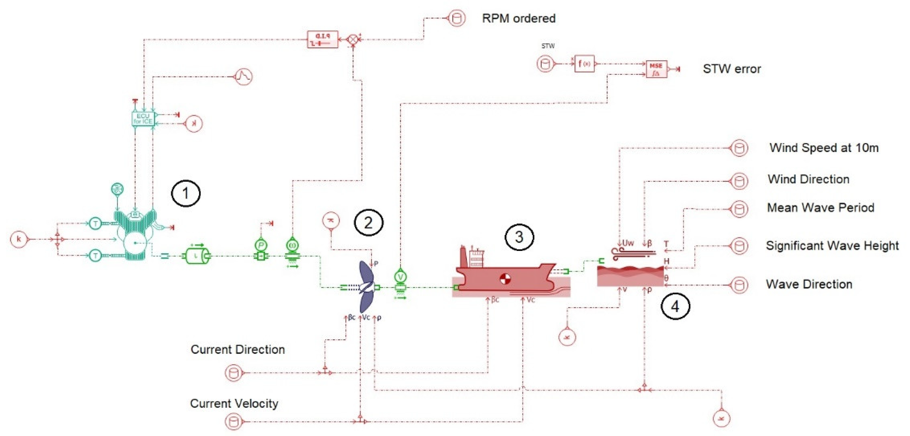
A digital twin of the case study ship was created with the use of Simcenter Amesim. Different modules from the marine library were implemented in order to simulate the behavior of the ship in actual conditions. Figure 6 presents the Amesim configuration that is used in this study.

The main modules that form the digital twin of the ship are as follows:

• Engine: Simulate the behavior of the propulsion engine of the ship. The main input parameter of this module is the rpm ordered by the crew.
• Propeller: Requires as input the engine power delivered through the shaft, the sea current direction and the sea current velocity. The output of the model is the thrust produced to overcome the total resistance for the ship movement. The model characterization of the propeller used is the first-quadrant—Wageningen B-series [35].
• Ship: Simulates the resistance of the ship in calm weather resistance according to the ship’s design. The resistance model used by the model is Holtrop and Mennen’s [36].
• Weather conditions module: Simulates the added resistance of the ship due to the weather conditions. Receives as input the wind speed at a 10 m height above the sea, the wind direction, the mean wave period, the significant wave height and the wave direction. For the air drag coefficient, the computation model used is IMO 2012, and the wave resistance model used is STAwave-2 [37].

The aforementioned blocks of models are interconnected according to the actual physical relations that exist between them, and based on the first principles (the equilibrium of mass, torque and energy), the integrated simulation model (the digital twin of the ship examined) can predict the ship through water (STW) velocity of the ship that corresponds to the input operating parameters provided at each time instant, based on the available dataset from the ADLM system used in the current study. Comparing the theoretical (predicted by the model) STW ship speed with the logged one (derived using the onboard speed log system), the mean square error is determined.

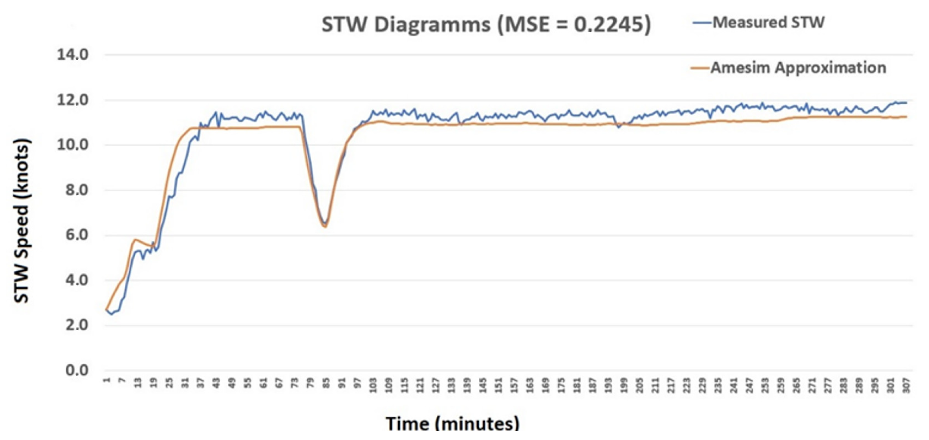
In order to validate the digital twin of the case study ship that we created using Amesim, we simulated the STW using data that belong to the first of the trips that are available to us. Using these data, we can check how close Amesim approximates the values of the measured STW in the case study reference conditions. Figure 7 presents the comparison between the measured STW values with the onboard sensor and the corresponding predicted ones using the model developed with the Amesim platform, during the first time series being examined.

As observed, the predicted values are close to the measured ones during the whole time period examined, which is a strong indication that the developed model manages to correctly predict, at least qualitatively, the effect of operating conditions on the value of STW. Moreover, the absolute values are very close to the measured ones, with the MSE value being equal to 0.2245.

5. Results and Discussion

To evaluate the performance of the aforementioned time series forecasting algorithms to compensate for missing sensor values or drifted values in a real ship scenario, the ship’s speed through water (STW) was set as a label parameter since this has a dominant effect on a ship’s fuel consumption, which is of the utmost importance for ship operators and ship owners. Another very important reason for choosing STW as the label is the fact that any sensor responsible for measuring STW, regardless of its type, is outside of the hull and exposed to the harsh environment of the sea. This makes these sensors more prone to drift. One other note is that one can argue that since Amesim or any other simulation software can estimate the STW, why bother using time series forecasting models? The answer to this question is that exactly the same procedure that is proposed in this paper, with the same expected results, can be used to predict any other sensor data that might be completely missing, even the ones that are crucial inputs for the simulation software to work. Creating virtual sensors with time series forecasting models might be the answer to increasing the robustness of an overall performance monitoring system.

The aforementioned time series algorithms predict the STW speed of a ship using all the available logged data following a gradually time-evolving procedure covering the full time period of the available dataset. A total of three cases were examined: in the first case, each algorithm predicts at each time step the value of the STW speed based on all the previous data available until that time, and this value is assumed to be known in the next time step until all the time period under investigation is covered (forecast horizon = one). In each iteration, past (known/estimated) data are increased with the forecast horizon. This type of prediction takes place in real-time.

In the second case, the prediction of the STW speed is estimated in batches of five values (forecast horizon = five). After each group of 5 time instants (t = 5), the STW speed values corresponding to each one of the past 5 time instants (t = 0 to t = 4) are predicted. In the following iteration of the prediction procedure (i.e., at t = 10), the already predicted STW speed values of the last predicted group of data (until t = 4) are used to predict the following group of 5 values (i.e., from t = 5 to t = 9). This procedure is then repeated in the next batch and so on. This type of prediction is near to real-time but has the advantage that algorithms have future knowledge of all the independent attribute values.

The third case is similar to the second with the difference that each batch expands to nine values (forecast horizon = nine). The limit of the examined forecast horizon to values between five and nine was purposely set due to the high computational demand of ANN algorithms and the corresponding time needed to provide results. Taking into account that in the use case examined, the ADLM system has a sampling frequency of 0.017 Hz, the calculations should be completed in less than 60 s with a forecast horizon of 1. In the cases of forecast horizons of five and nine, the available time increases by a factor of five and nine, respectively. The latter is crucial, especially in cases where CPU power is limited (which is the case, for example, when these techniques should be applied for specific applications onboard).

The predicted values of STW speed according to each of the above three data interpretation approaches (with forecast horizons of one, five and nine) using each of the four algorithms presented (LR, RF, LSTM and N-Beats), along with the measured values from the o-board speed log sensor, were compared with the assumed as “true” value of the STW speed predicted via the digital twin of the ship (physical simulation model) for the corresponding operating conditions. The parameter used to compare these values and evaluate the performance of each of the approaches presented in compensating for the missing data and the drift in the readings of the STW sensors is the mean squared error (MSE). More specifically, considering that the predicted values of the STW speed based on the developed simulation model are independent of the possible causes that could lead to the STW log sensor’s failure or drift, it is suitable to assume that these predictions could be treated as being closest to the unbiased real STW speed value for each operating condition. Therefore, this value is used for the definition of the MSE when the various approaches proposed in the present study are evaluated, and high values of MSE could be attributed to the low effectiveness of a certain approach to compensate for STW sensor drift or loss of data. In this way, it becomes possible to compare the various approaches objectively, although it the actual/accurate value of the STW at each operating condition is unknown.

5.1. Data Pre-Processing—Time Series Forming

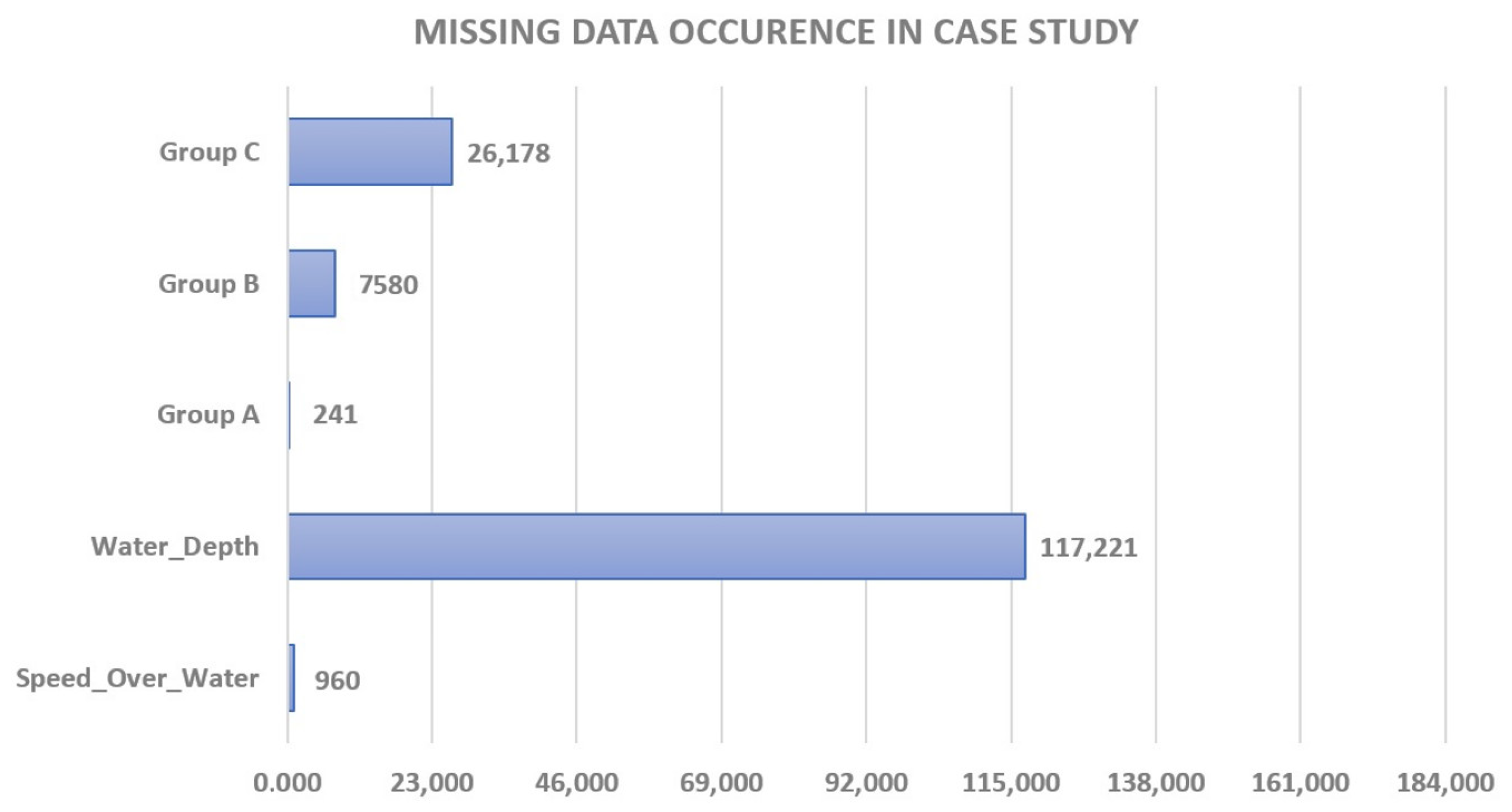
In the first step for all the instances, from the data collected with the ship’s ADLM system, speed over ground (SOG) values of less than 2 knots were discarded because they were considered to correspond to transition periods or periods in which the ship was in harbor.

From the original set of available attributes (logged parameters), only those related (directly or indirectly) to the parameter under study (STW) were taken into account. All other (irrelevant) attributes (e.g., parameters related to the auxiliary engines, or data used to monitor the operating conditions of the auxiliary pipe network) were excluded from the dataset in order to reduce the total volume of the data and thus maximize the prediction accuracy of the ML models that were used. Following this approach, the total number of attributes taken into account decreased from the original 178 entries to 49.

In the second step, all the attributes that have an extremely high correlation with STW and originate from the same sensor were excluded. Therefore, longitudinal water speed, transverse water speed and stern transverse water speed were excluded from the dataset since they could bias the results.

Afterward, all the instances that had missing values for attributes related to meteorological conditions and in which missingness was continuous for very long time spans were also excluded from the dataset used. This eliminated the possible bias of the dataset that would arise with any kind of interpolation technique applied.

Especially for the attribute “Water depth” (which might affect the way that an STW sensor works), interpolation was applied in cases where there was continuality between the last non-missing value and the first non-missing value. The criterion used for determining the continuality of the missing values was the percentage of the difference between the last and first consecutive non-missing values, which was set to be as high as 3%. The threshold of 3% was set since this is the typical accuracy of this type of sensor [38]. For those entries where continuality criterion checks failed or the number of continuous missing values was high enough, they were excluded from the final dataset used.

5.2. Algorithm Training/Hyperparameter Optimization

After the above preprocessing, 53 separate time series data (each of them corresponding to a different trip of the ship) were created, with no missing values, that span from 13 February 2020 until 20 July 2020. These time series can be separated into two periods. The first 26 time series represent continuous trips with minimum harbor periods that span from February to April. From the 27th time series until the 53rd, the ship started to increase the periods of staying in harbors. Due to the fact that marine growth mainly develops when a ship is stationary and, thus, the possibility of affecting the accuracy of the STW sensor increases, we decided to use the first 26 time series for the training of all the algorithms and test with the dataset corresponding to the second period. In this way, the ability of the algorithms to compensate for both missingness and sensor drift can be evaluated.

The time series forecasting needed for this paper was conducted using Python scripts that utilize well-known and established libraries in the area of ML. A relatively new Python library (Darts) simplified the code to a great extent and has been proven to be very helpful. Darts is an open-source Python library created by Unit8 that uses scikit-learn as a back-bone and can be used for forecasting time series [39].

The hardware/software used to perform the necessary calculations in this study were made common for all the algorithms examined to make the time comparisons reliable. The configuration that was used is presented in

Table 2. Hardware/software configuration.

Component	Specs
CPU	AMD Ryzen 9 5900X
RAM	128GB Dual Chanell DDR4
GPU	Nvidia RTX 3060Ti 8GB (Cuda-enabled)
Operating system	Windows 10 Pro
IDE	PyCharm
Python version	3.9.13
Python libraries	Darts, Pytorch, Pandas and NumPy

. (It is worth noting that the intelligence that is now feasible to be implemented and integrated into our systems is mainly attributed to the hardware capabilities, which in the near past could not easily support protocol processing execution [40].)

The training of any ML algorithm is, basically, the procedure in which a number of parameters are learned from the data. We used existing data in order to fit the model parameters. In every ML model (including the ones used for time series forecasting), there is another kind of parameter that cannot be directly learned from the regular training process. These parameters, which are called hyperparameters, are model-specific and must be determined before the learning process begins. These kinds of parameters determine the important properties of each model, such as its complexity or how fast it can learn from data. For this implementation, we determined the best hyperparameters using the grid search technique for the Linear Regression and Random Forest algorithms and the random search technique for LSTM and N-Beats in each of the 26 time series (1st period) that were used for algorithm training.

In the grid search hyperparameter tuning, we defined a search space as a grid of hyperparameter values and evaluated every position in the grid, while in the random search, we defined a search space as a bounded domain of hyperparameter values and randomly samples points in that domain [41]. The above separation was dictated by the fact that the LSTM and N-Beats algorithms completed the grid search for the hyperparameters in a test time series over unacceptably long time periods due to the extensive calculations needed. In

Table 3. Times for completion of grid search.

Algorithm	Time (s)
Linear Regression (LR)	12
Random Forest (RF)	287
LSTM	33,649
N-Beats	219,070

, the average time needed for a grid hyperparameter search for the Linear Regression and Random Forest algorithms together with the corresponding time for a random time series when using LSTM and N-Beats are presented.

In Table 3, we can witness the exponential increase in the computational time when using the ANN models. The final set of hyperparameters that were used for the combined model (the one that used all of the 26 time series for training) was constructed with the use of the median of each separate hyperparameter in the cases of the Linear Regression and Random Forest algorithms and the corresponding results of the random search in the cases of LSTM and N-Beats.

In each of the three test cases examined (i.e., with forecast horizons of one, five and nine) and for all of the time series that were used for training, we calculated the MSE that the algorithms had when predicting the STW. The last 10% of the values of STW in each time series were used for testing. This was carried out in order to evaluate the performance of the algorithms in terms of consistency. 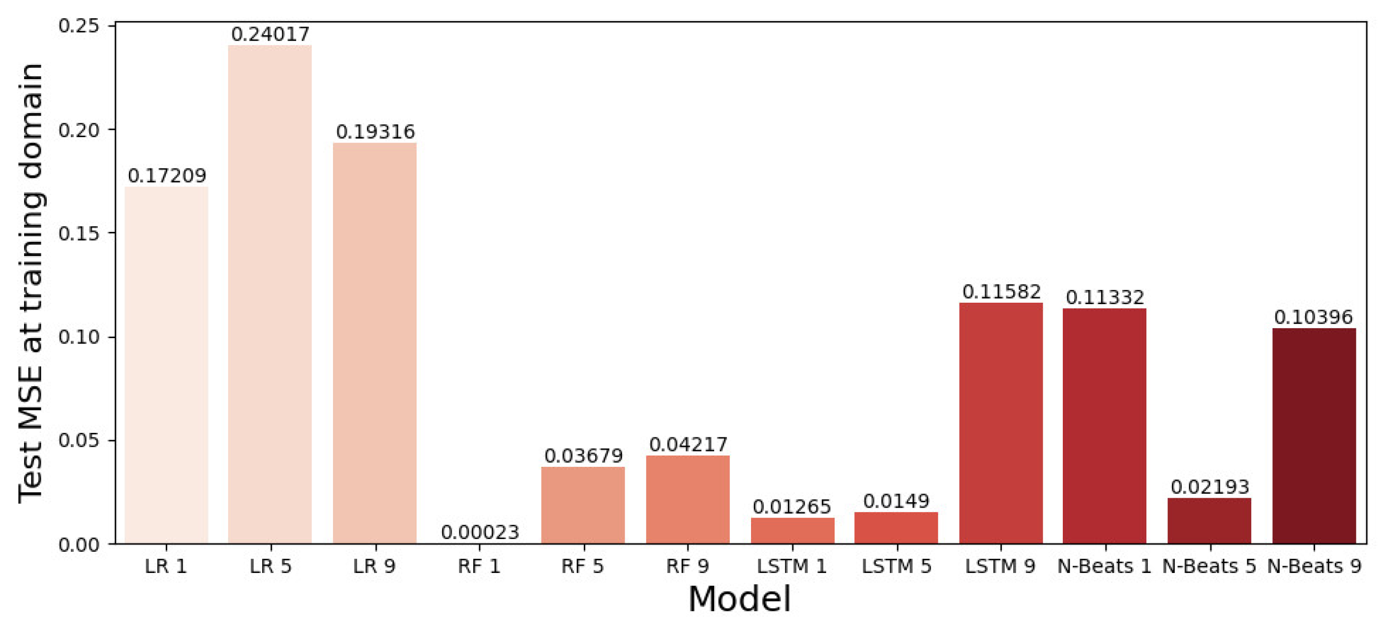Figure 8 presents the allocation of mean MSE values for the prediction of STW for all four algorithms used (LR = Linear Regression model and RF = Random Forest model).

In Figure 8, it is observed that the absolute best performance in terms of the MSE corresponds to the Random Forest (RF) algorithm when setting the forecasting horizon equal to one. The MSE = 0.00023 observed in this case is an exceptional value, meaning that the total amount of data from the 26 time series are sufficient enough to train this algorithm without overfitting the data. On the other hand, the Linear Regression algorithm (an algorithm that is commonly used for data imputation) is not able to fit the data very well, presenting by far the worst performance, regardless of the forecast horizon. The more sophisticated and computationally demanding ANN algorithms (LSTM and N-Beats) accomplished very good performances (with LSTM outperforming in all cases) but cannot outperform the Random Forest algorithm, which seems to be the most suitable algorithm of all. Finally, it is worth noting that, with the exception of the N-Beats algorithm, the best MSE value is achieved when the forecast horizon is set to one. This means that “future knowledge” of the attributes at the time of prediction (which is used in the case of the time horizon at five and nine) does not increase their performance.

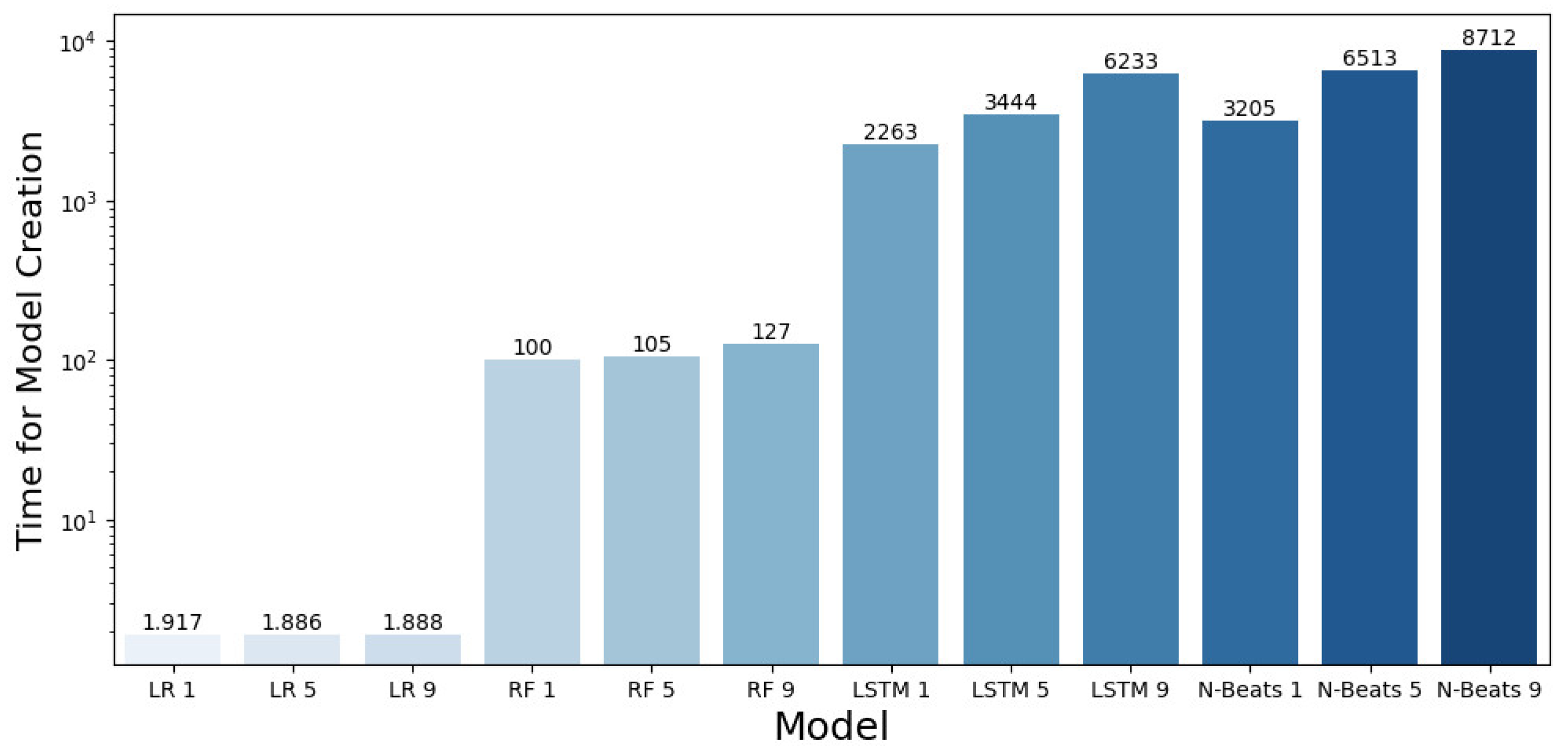
In Figure 9, we present the CPU time needed for model creation in each of the twelve cases examined (three cases of time horizons for each of the four algorithms evaluated). It should be noted that the y-axis (time spent in seconds) is on a log scale.

As expected, the increase in the model complexity resulted in more computational demands, which in turn led to an increase in the time needed to complete the necessary calculations for model creation. The increase in the time needed in the cases of LSTM and N-Beats is exponential compared with that in the LR and RF cases. The average time for completion of LSTM is one 1 h and 6 min, while Random Forest has an average time of 1 min and 50 s. Combining these results with the comparison of the MSE values shown in Figure 8, it is concluded that Random Forest proved to be among the most accurate algorithms with the lowest CPU demand, which makes it preferable for the application examined. Moreover, from Figure 8, it is observed that the increase in the forecast horizon does not improve the completion time as could be expected, although this leads to fewer iterations needed from the algorithms.

5.3. Algorithm Evaluation

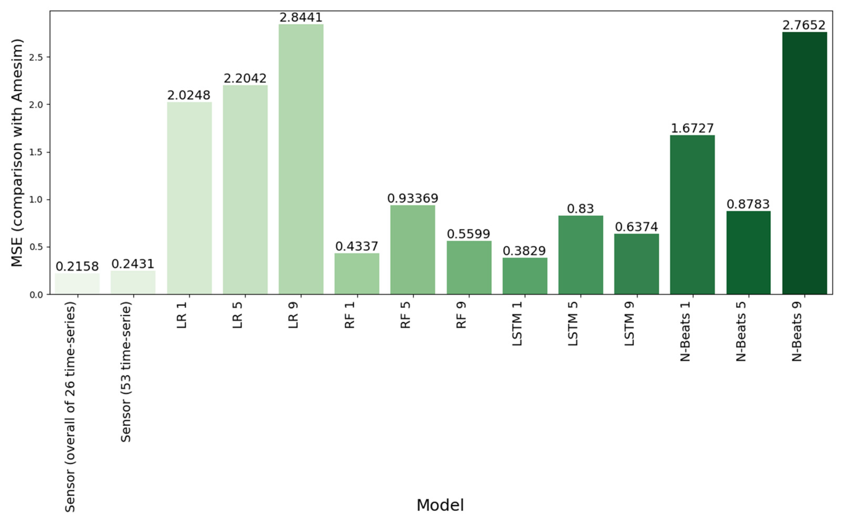
After validating the models’ performances, their evaluation in the 2nd period of the ship cruising data (and, specifically, the 53rd time series) is presented in Figure 10. As already explained, the criterion for this evaluation is the MSE defined using the predicted value of the STW for each variant of the model being examined and the corresponding value predicted with the Ship Digital Twin model (Amesim) for the same conditions. Moreover, in the same figure, the MSE for the sensor is presented, which is derived using the recorded actual value with the onboard installed STW sensor and the corresponding value predicted with the physical model (Amesim), which is assumed to be independent of any parameter that could cause sensor drift or missing values. In Figure 10, we can witness an increase in the MSE values between the digital twin and the STW values measured with the sensor when we switch from the first period to the test period (the MSE increases from 0.2158 to 0.2431), which indicates that there is a slightly increasing drift, as observed, and the MSE of the sensor is very low (equal to 0.2431), which is an indication that in the specific time period examined (2nd period), the STW sensor does not suffer from high drift.

On the other hand, when focusing on the performance of the Random Forest method with a forecast horizon of one (RF-1), which was identified as having the best performance in terms of MSE when tested in the first time domain (the twenty-six time series used for training), it seems that in the second time series (representing the actual test conditions), it has the second best MSE value and is outperformed by the LSTM model with the same forecast horizon (LSTM-1). This indicates that the LSTM model can generalize better in the domain adaptation. Both the Random Forest model and LSTM model achieved comparable MSE values with the sensor readings, which implies that both models can compensate for the complete missingness of STW data; however, this score is not considered good enough to indicate that these algorithms could also be used to compensate for the error induced by sensor drift. On the other hand, the LR model seems to have the worst performance, followed by N-Beats.

6. Conclusions and Future Perspectives

Most new ship buildings are equipped with modern data acquisition, control and monitoring systems that collect data from various sensors installed onboard, and analyze and combine these data with meteorological and geographical data provided by external sources, to assist shipping companies to minimize their operating expenses and become more competitive by optimizing ship performance. One of the most important metrics that is logged by the ADLM system and used for the analysis of ship performance is the ship’s speed through water (STW), which is directly related to the propulsion power needed during cruising. This is why this parameter was selected to evaluate the performance of four widely used time-series forecasting algorithms (with three variants for each) in compensating for missing data and drift in the readings of STW sensors, which is a common problem in real-life applications.

The four selected time series forecasting algorithms have escalating complexity in dealing with the complete missingness of STW data or the degradation of STW reading accuracy due to drift. All four algorithms were tested in three different configurations, i.e., in real-time prediction (forecast horizon = one) and near-to-real-time prediction (forecast horizon = five and forecast horizon = nine). The predictions as well as the onboard STW sensor readings were compared in terms of MSE with the assumed “ground truth” STW value predicted with the physical model of the ship developed using the Siemens Amesim simulation platform.

The results indicate that an ensemble model (Random Forest) and the LSTM Recurrent Neural Network, if used recurrently to predict only the next label value (forecast horizon = one), are able to generalize well and predict STW with adequate accuracy when trained in a certain domain (with the ship and STW sensor under certain reference conditions in terms of calibration and hull degradation) and tested in a different domain (with the ship and STW sensor in real-life operational test cases over a long time period).

The MSE scores for the STW for the above 2 algorithms (RF and LSTM) were 0.3829 and 0.4337, respectively, while the corresponding value for the sensor readings was equal to 0.2431. This high difference is an indication that these algorithms cannot be used or at least do not offer high confidence in solving the crucial problem faced in real-life occurrences of sensor drift or missing values. Based on the results, it seems that using a physical model could be a challenging alternative, at least in cases where this could be possible (i.e., the data required for the model are available). However, it should be noted that also in the case of using a physical simulation model, as was carried out in the present study to “generate” the unbiased reference value of STW for each operating condition, the effect of the model accuracy must be considered. In real-life applications, the STW value depends on many parameters, often being difficult to be precisely determined and simulated, especially if the results are needed in real-time. Even if using more detailed simulation approaches, using computational fluid dynamics (CFD) is not expected to provide a better solution to the scope of this study. Therefore, the use of simple physical models based on the first principles seems to be a fair compromise. The next steps include the investigation of more specialized techniques for domain adaptation, such as RNN autoencoders.