
PECSO: An Improved Chicken Swarm Optimization Algorithm with Performance-Enhanced Strategy and Its Application


Abstract
:1. Introduction
- A hierarchy using a free grouping mechanism is proposed, which not only bolsters the diversity of individuals within this hierarchy but also enhances the overall search capability of the population;
- Synchronous updating and spiral learning strategies are implemented that fortify the algorithm’s ability to sidestep local optima. This approach also fosters a more efficient balance between exploitation and exploration;
- PECSO algorithm exhibits superior global search capability, faster convergence speed and higher accuracy, as confirmed by the CEC2017 benchmark function;
- The exceptional performance of the PECSO algorithm is further substantiated by its successful application to two practical problems.
2. Chicken Swarm Optimization Algorithm
3. Improved CSO Algorithm
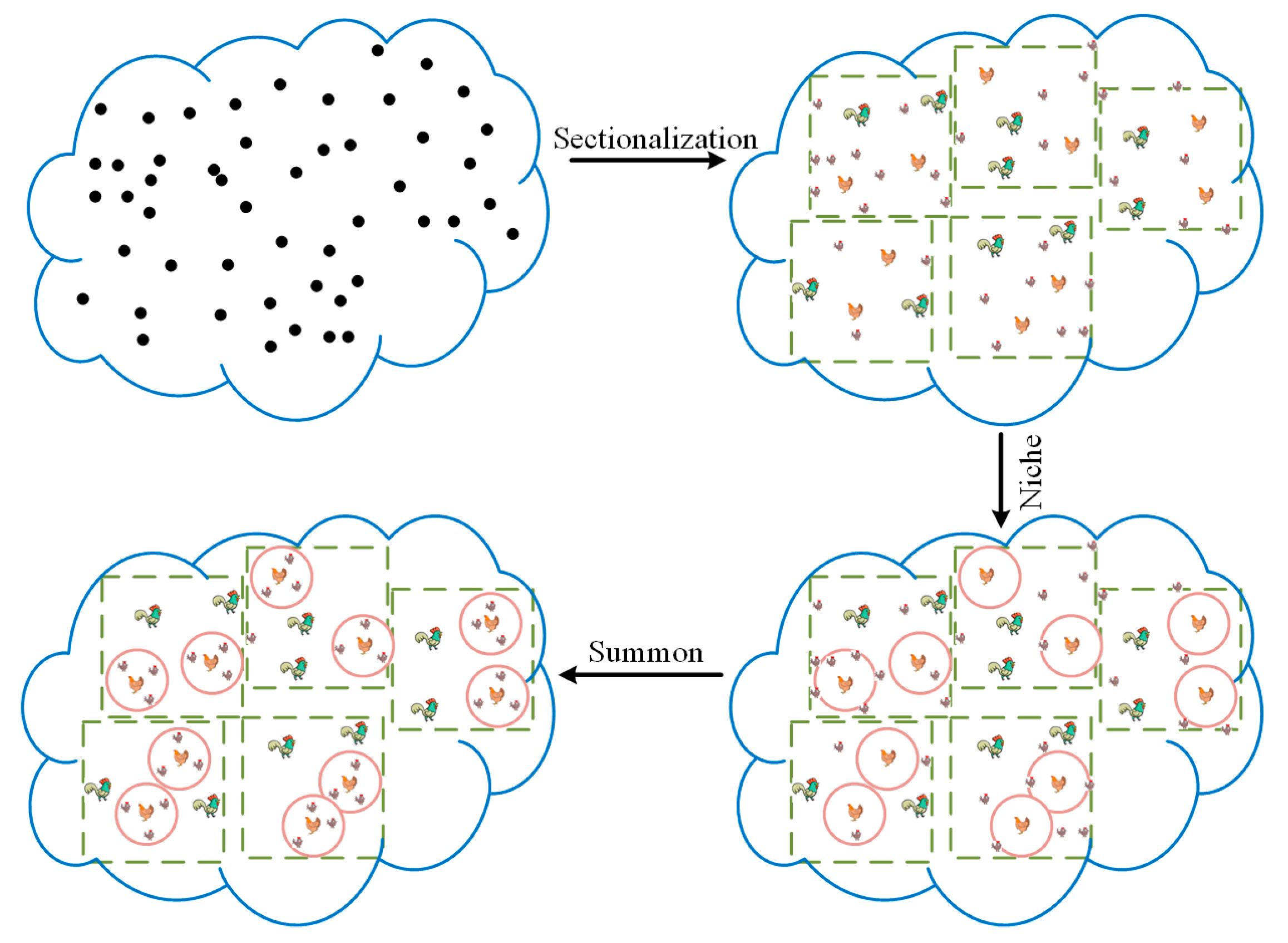
3.1. New Population Distribution
3.2. Individual Updating Methods
3.2.1. Best-Guided Search for Roosters
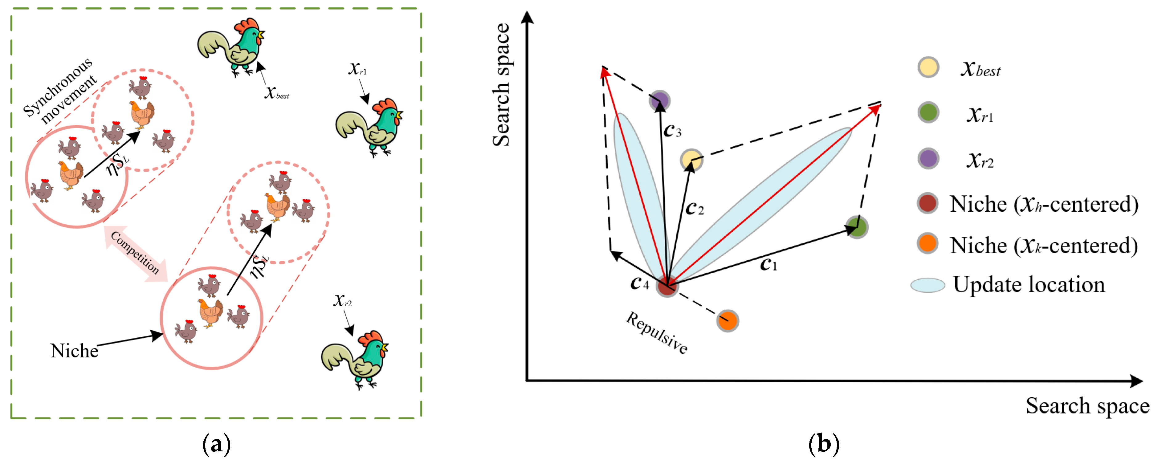
3.2.2. Bi-Objective Search for Hens
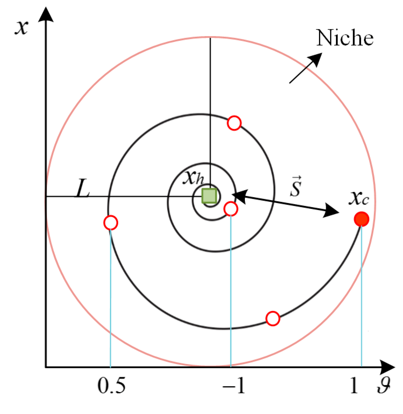
3.2.3. Simultaneous and Spiral Search for Chicks
3.3. The Implementation and Computational Complexity of PECSO Algorithm
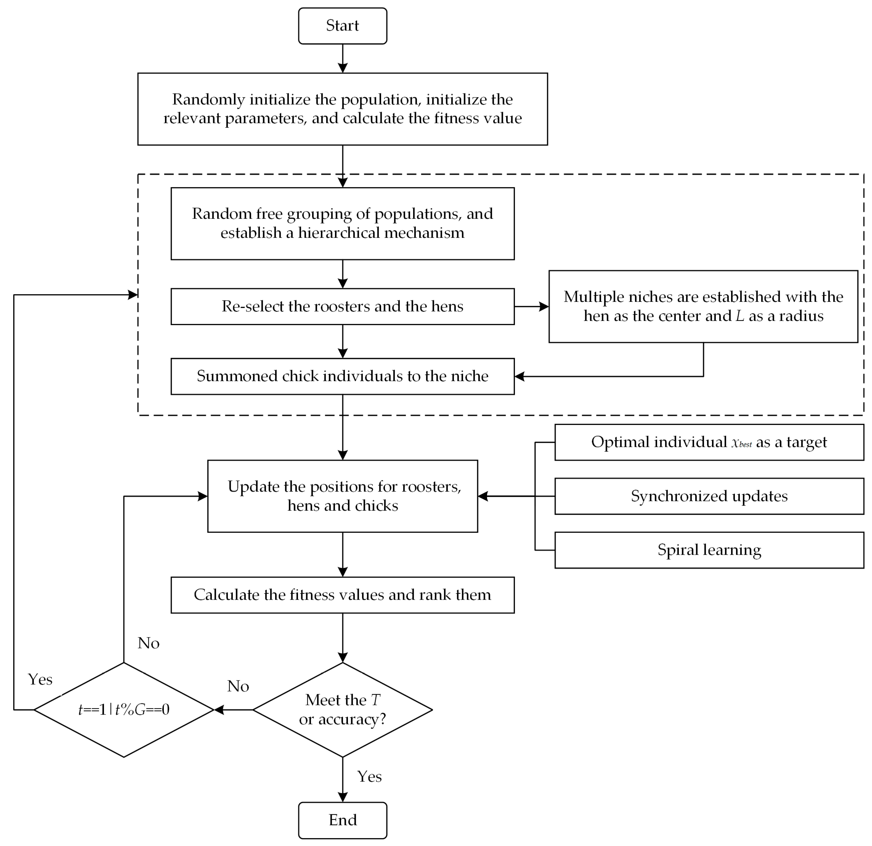
3.3.1. The Implementation of PECSO Algorithm
| Algorithm 1: Pseudocode of PECSO algorithm |
| Initialize a population of N chickens and define the related parameters; While t < Gmax If (t % G == 0) Free grouping of populations and selection of roosters and hens within each group based on fitness values; Many niches are established with the hens as the center and L as the radius, according to Equations (5) and (6); Chicks are summoned by hens within the niche to recreate the hierarchy mechanism and to mark them. End if For i = 1: Nr Update the position of the roosters by Equation (8); End for For i = 1: Nh Synchronous update step of the niche is calculated by Equation (9); Update the position of the hens by Equation (10); End for For i = 1: Nc Spiral learning of chicks by Equation (11); Update the position of the chicks by Equation (12); End for Evaluate the new solution, and update them if they are superior to the previous ones; End while |
3.3.2. The Computational Complexity of PECSO Algorithm
4. Simulation Experiment and Result Analysis
4.1. Experimental Settings
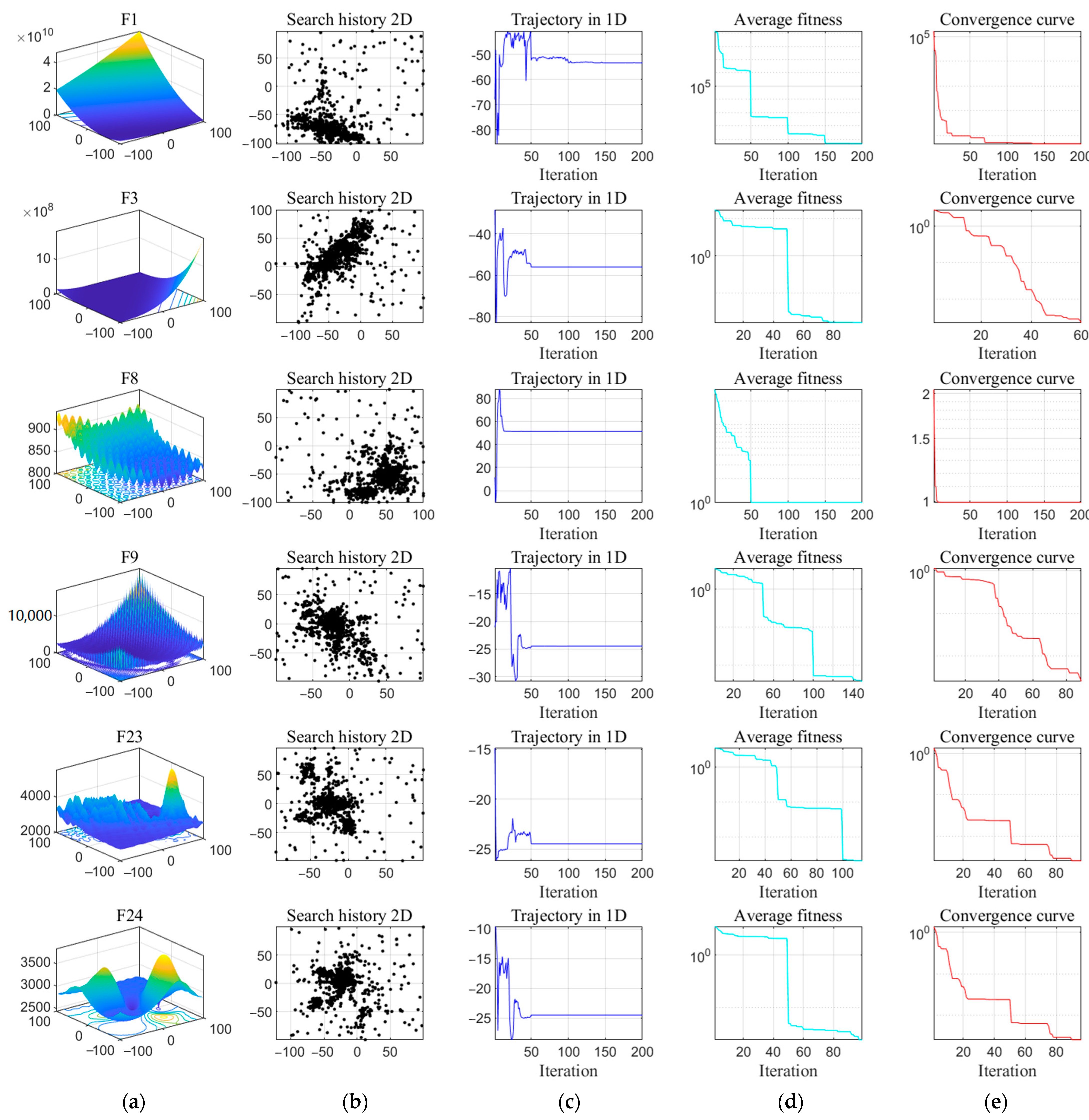
4.2. Qualitative Analysis
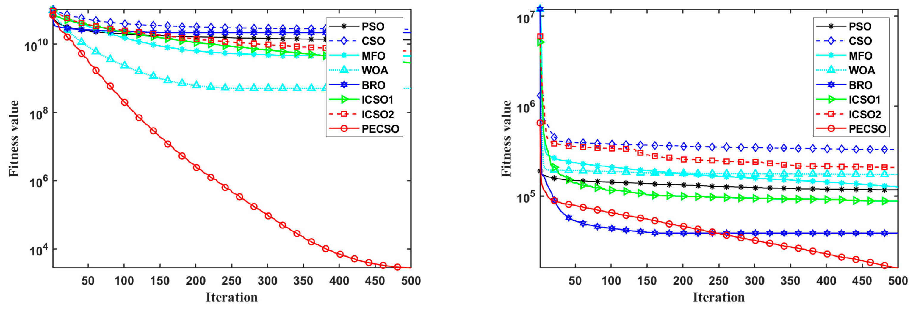
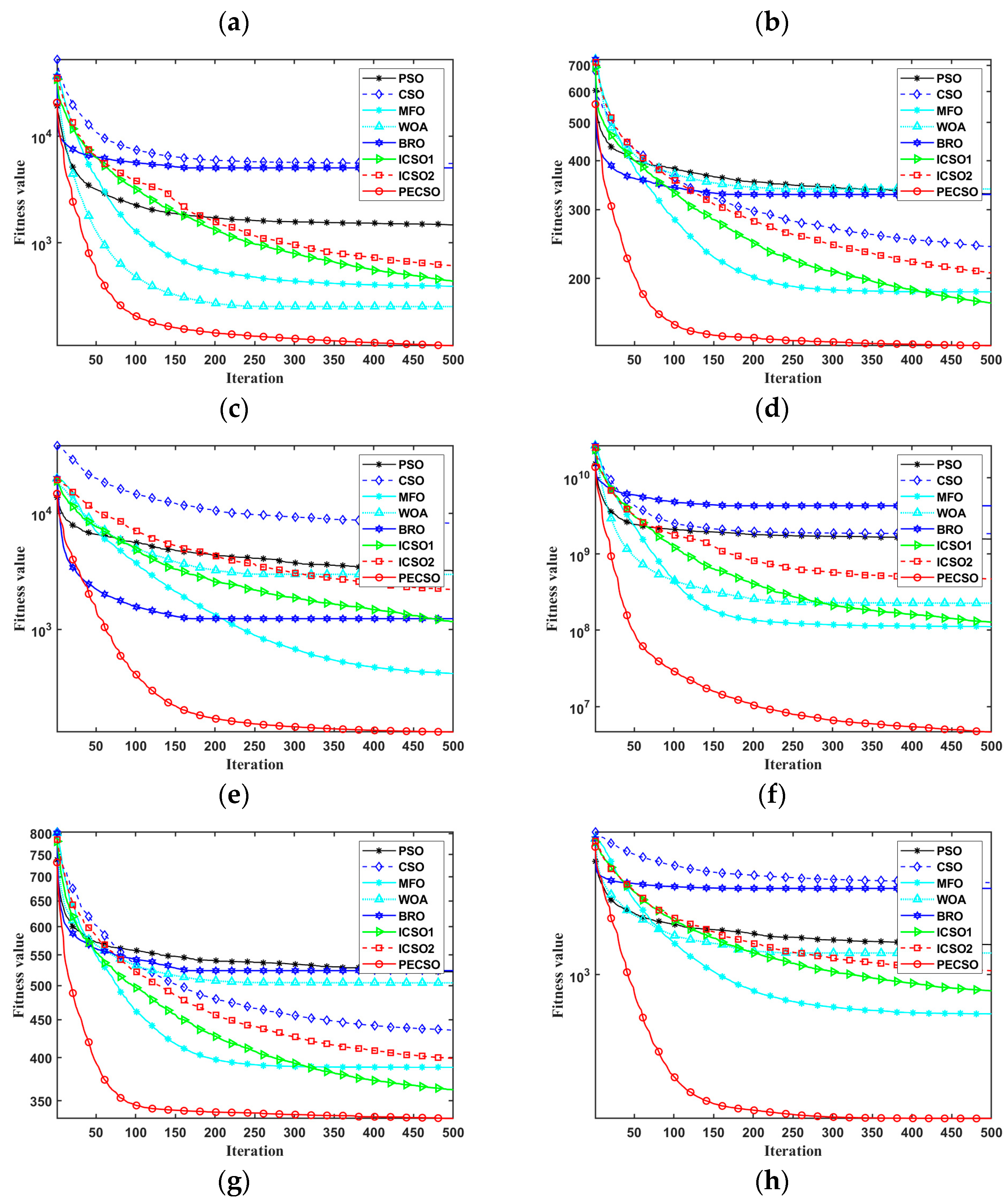
4.3. Quantitative Analysis
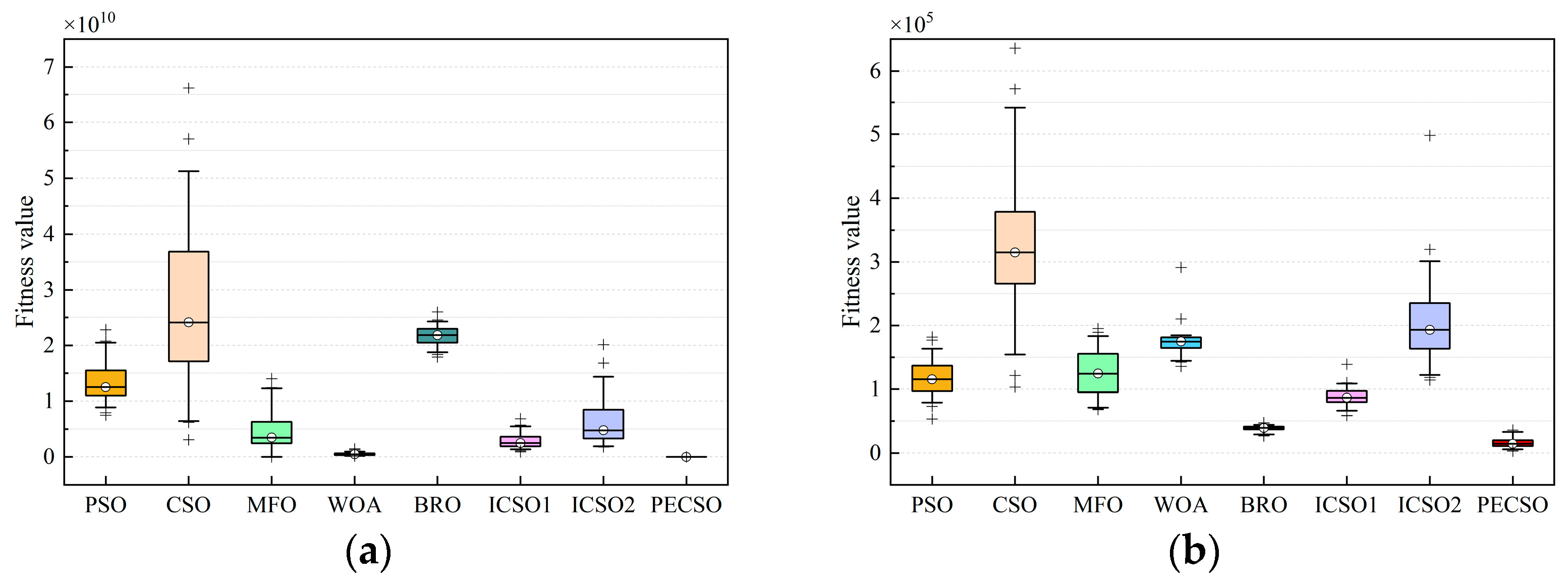
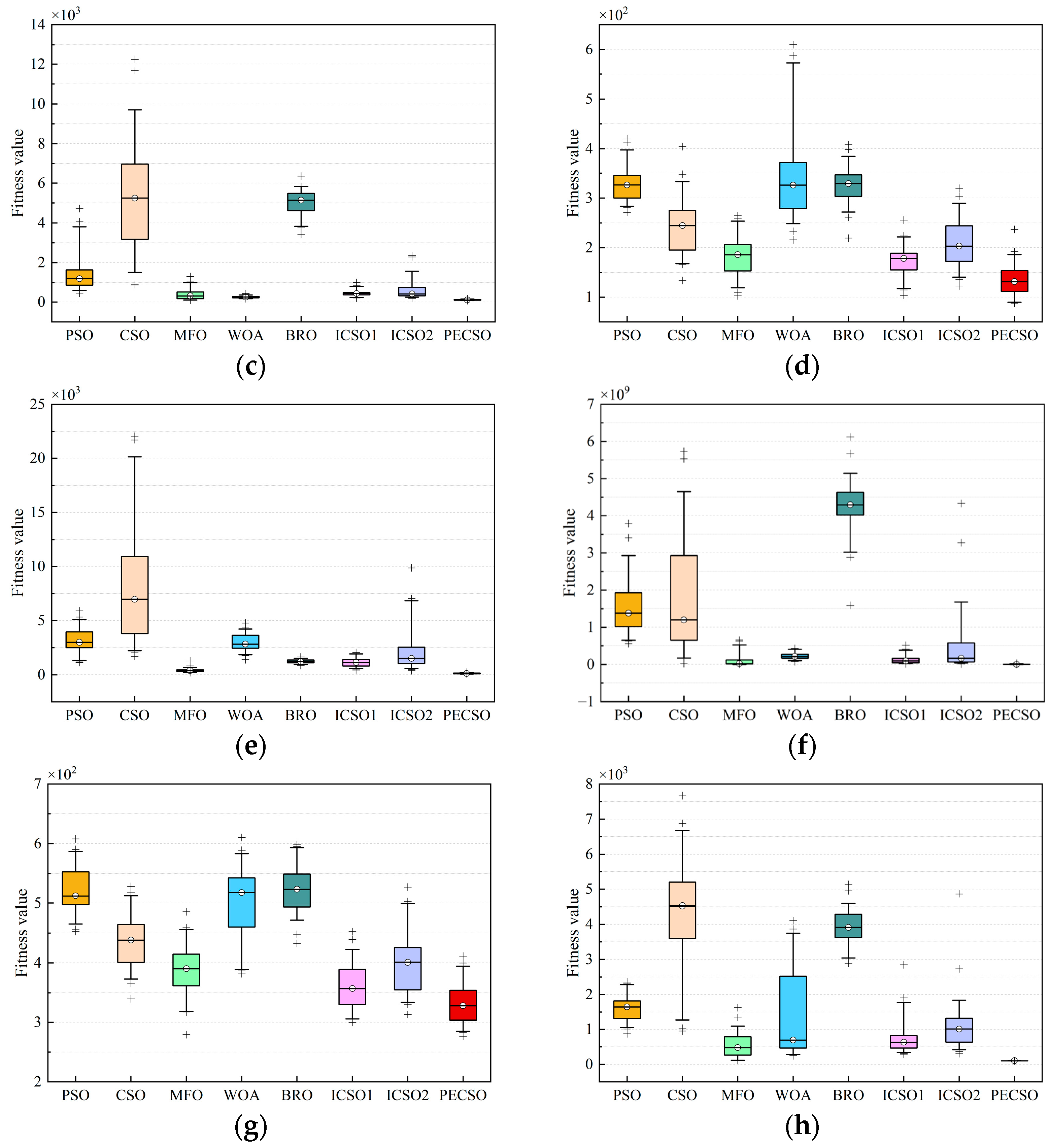
- From the unimodal and multimodal functions, we can find that the PECSO algorithm achieves the minimum mean and standard deviation. From the hybrid and composition functions, the PECSO algorithm obtained the best value of 80%. This shows that the PECSO algorithm has high convergence accuracy and strong global exploration ability, and its computing performance is more competitive;
- The experimental results show that the solving ability of unimodal and multimodal functions is not affected by dimensional changes, while hybrid and composite functions get more excellent computational results in higher dimensions. This indicates that the PECSO algorithm can balance the exploitation and exploration well and has a strong ability to jump out of the local optimum. The possible reason is that the free grouping mechanism improves the establishment of the hierarchy and increases the diversity of roosters in the population. Meanwhile, synchronous updating of individuals in niche and spiral learning of chicks can effectively improve the exploitation breadth and exploration depth of the PECSO algorithm;
- The running time of the PECSO algorithm is slightly higher than that of the CSO algorithm, but they have the same order of magnitude. It shows that the PECSO algorithm effectively improves computational performance;
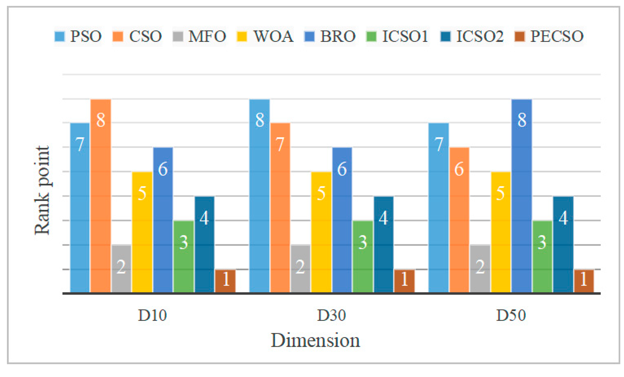
- We rank the test results of all algorithms on the benchmark function, and the average value is the indicator. Figure 6 finds that the convergence results of the PECSO algorithm are outstanding in different test dimensions.
5. Case Analysis of Practical Application Problems
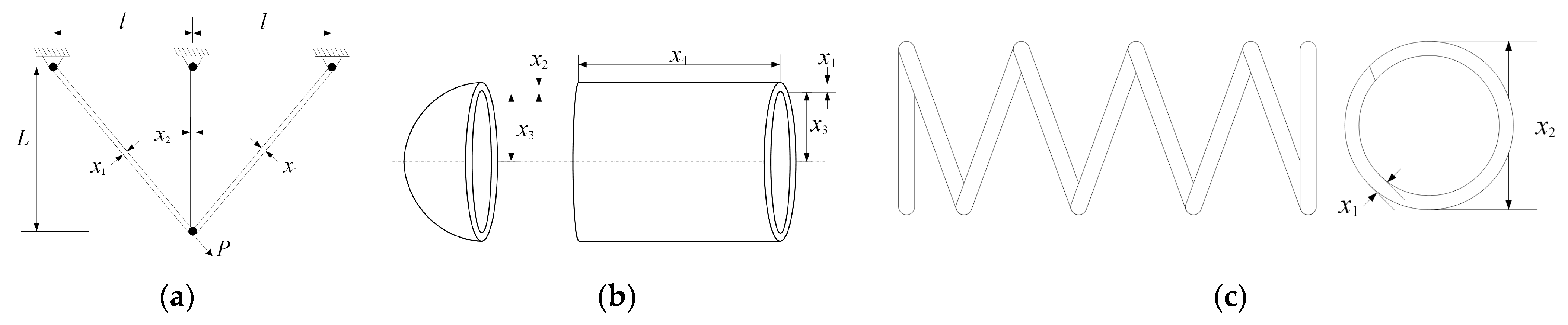
5.1. Engineering Optimization Problems
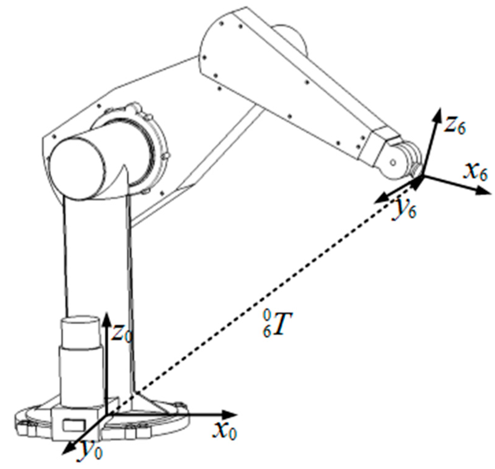
5.2. Solve Inverse Kinematics of PUMA 560 Robot
5.2.1. Kinematic Modeling and Objective Function Establishment
5.2.2. Simulation Experiment and Analysis
6. Conclusions
Author Contributions
Funding
Institutional Review Board Statement
Data Availability Statement
Conflicts of Interest
References
- Kumar, N.; Shaikh, A.A.; Mahato, S.K.; Bhunia, A.K. Applications of new hybrid algorithm based on advanced cuckoo search and adaptive Gaussian quantum behaved particle swarm optimization in solving ordinary differential equations. Expert Syst. Appl. 2021, 172, 114646. [Google Scholar] [CrossRef]
- Kennedy, J.; Eberhart, R. Particle swarm optimization. In Proceedings of the ICNN’95-International Conference on Neural Networks, Perth, Australia, 27 November–1 December 1995; Volume 4, pp. 1942–1948. [Google Scholar]
- Mirjalili, S. Genetic algorithm. In Evolutionary Algorithms and Neural Networks: Theory and Applications; Springer: Cham, Switzerland, 2019; Volume 780, pp. 43–55. [Google Scholar]
- Yang, X.S. A New Metaheuristic Bat-Inspired Algorithm. In Nature Inspired Cooperative Strategies for Optimization (NICSO 2010). In Studies in Computational Intelligence; González, J.R., Pelta, D.A., Cruz, C., Terrazas, G., Krasnogor, N., Eds.; Springer: Berlin/Heidelberg, Germany, 2010; Volume 284, pp. 65–74. [Google Scholar]
- Cuevas, E.; Cienfuegos, M.; Zaldívar, D.; Pérez-Cisneros, M. A swarm optimization algorithm inspired in the behavior of the social-spider. Expert Syst. Appl. 2013, 40, 6374–6384. [Google Scholar] [CrossRef] [Green Version]
- Meng, X.; Liu, Y.; Gao, X.; Zhang, H. A new bio-inspired algorithm: Chicken swarm optimization. In Proceedings of the International Conference in Swarm Intelligence, Hefei, China, 17–20 October 2014; pp. 86–94. [Google Scholar]
- Mirjalili, S. Moth-flame optimization algorithm: A novel nature-inspired heuristic paradigm. Knowl.-Based Syst. 2015, 89, 228–249. [Google Scholar] [CrossRef]
- Mirjalili, S.; Lewis, A. The whale optimization algorithm. Adv. Eng. Softw. 2016, 95, 51–67. [Google Scholar] [CrossRef]
- Faramarzi, A.; Heidarinejad, M.; Mirjalili, S.; Gandomi, A.H. Marine predators algorithm: A nature-inspired metaheuristic. Expert Syst. Appl. 2020, 152, 113377. [Google Scholar] [CrossRef]
- Rahkar Farshi, T. Battle royale optimization algorithm. Neural Comput. Appl. 2021, 33, 1139–1157. [Google Scholar] [CrossRef]
- Guha, R.; Ghosh, S.; Ghosh, K.K.; Cuevas, E.; Perez-Cisneros, M.; Sarkar, R. Groundwater flow algorithm: A novel hydro-geology based optimization algorithm. IEEE Access 2022, 10, 132193–132211. [Google Scholar] [CrossRef]
- Chen, Z.; Francis, A.; Li, S.; Liao, B.; Xiao, D.; Ha, T.T.; Li, J.; Ding, L.; Cao, X. Egret Swarm Optimization Algorithm: An Evolutionary Computation Approach for Model Free Optimization. Biomimetics 2022, 7, 144. [Google Scholar] [CrossRef]
- Dehghani, M.; Montazeri, Z.; Trojovská, E.; Trojovský, P. Coati Optimization Algorithm: A new bio-inspired metaheuristic algorithm for solving optimization problems. Knowl.-Based Syst. 2023, 259, 110011. [Google Scholar] [CrossRef]
- Wu, H.; Zhang, X.; Song, L.; Zhang, Y.; Gu, L.; Zhao, X. Wild Geese Migration Optimization Algorithm: A New Meta-Heuristic Algorithm for Solving Inverse Kinematics of Robot. Comput. Intel. Neurosc. 2022, 2022, 5191758. [Google Scholar] [CrossRef]
- Trojovská, E.; Dehghani, M.; Leiva, V. Drawer Algorithm: A New Metaheuristic Approach for Solving Optimization Problems in Engineering. Biomimetics 2023, 8, 239. [Google Scholar] [CrossRef]
- Hashim, F.A.; Hussien, A.G. Snake optimizer: A novel meta-heuristic optimization algorithm. Knowl.-Based Syst. 2022, 242, 108320. [Google Scholar] [CrossRef]
- Azizi, M.; Talatahari, S.; Gandomi, A.H. Fire Hawk Optimizer: A novel metaheuristic algorithm. Artif. Intell. Rev. 2023, 56, 287–363. [Google Scholar] [CrossRef]
- Wang, J.; Zhang, F.; Liu, H.; Ding, J.; Gao, C. Interruptible load scheduling model based on an improved chicken swarm optimization algorithm. CSEE J. Power Energy 2020, 7, 232–240. [Google Scholar]
- Mu, Y.; Zhang, L.; Chen, X.; Gao, X. Optimal trajectory planning for robotic manipulators using chicken swarm optimization. In Proceedings of the 2016 8th International Conference on Intelligent Human-Machine Systems and Cybernetics, Hangzhou, China, 27–28 August 2016; Volume 2, pp. 369–373. [Google Scholar]
- Li, Y.; Wu, Y.; Qu, X. Chicken swarm–based method for ascent trajectory optimization of hypersonic vehicles. J. Aerosp. Eng. 2017, 30, 04017043. [Google Scholar] [CrossRef]
- Yu, X.; Zhou, L.; Li, X. A novel hybrid localization scheme for deep mine based on wheel graph and chicken swarm optimization. Comput. Netw. 2019, 154, 73–78. [Google Scholar] [CrossRef]
- Lin, M.; Zhong, Y.; Chen, R. Graphic process units-based chicken swarm optimization algorithm for function optimization problems. Concurr. Comput. Pract. Exp. 2021, 33, e5953. [Google Scholar] [CrossRef]
- Li, M.; Bi, X.; Wang, L.; Han, X.; Wang, L.; Zhou, W. Text Similarity Measurement Method and Application of Online Medical Community Based on Density Peak Clustering. J. Organ. End User Comput. 2022, 34, 1–25. [Google Scholar] [CrossRef]
- Zouache, D.; Arby, Y.O.; Nouioua, F.; Abdelaziz, F.B. Multi-objective chicken swarm optimization: A novel algorithm for solving multi-objective optimization problems. Comput. Ind. Eng. 2019, 129, 377–391. [Google Scholar] [CrossRef]
- Ahmed, K.; Hassanien, A.E.; Bhattacharyya, S. A novel chaotic chicken swarm optimization algorithm for feature selection. In Proceedings of the 2017 Third International Conference on Research in Computational Intelligence and Communication Networks, Kolkata, India, 3–5 November 2017; pp. 259–264. [Google Scholar]
- Deb, S.; Gao, X.Z.; Tammi, K.; Kalita, K.; Mahanta, P. Recent studies on chicken swarm optimization algorithm: A review (2014–2018). Artif. Intell. Rev. 2020, 53, 1737–1765. [Google Scholar] [CrossRef]
- Meng, X.B.; Li, H.X. Dempster-Shafer based probabilistic fuzzy logic system for wind speed prediction. In Proceedings of the 2017 International Conference on Fuzzy Theory and Its Applications, Pingtung, Taiwan, 12–15 November 2017; pp. 1–5. [Google Scholar]
- Wang, Y.; Sui, C.; Liu, C.; Sun, J.; Wang, Y. Chicken swarm optimization with an enhanced exploration–exploitation tradeoff and its application. Soft Comput. 2023, 27, 8013–8028. [Google Scholar] [CrossRef]
- Liang, X.; Kou, D.; Wen, L. An improved chicken swarm optimization algorithm and its application in robot path planning. IEEE Access 2020, 8, 49543–49550. [Google Scholar] [CrossRef]
- Wang, Z.; Zhang, W.; Guo, Y.; Han, M.; Wan, B.; Liang, S. A multi-objective chicken swarm optimization algorithm based on dual external archive with various elites. Appl. Soft Comput. 2023, 133, 109920. [Google Scholar] [CrossRef]
- Li, M.; Li, C.; Huang, Z.; Huang, J.; Wang, G.; Liu, P.X. Spiral-based chaotic chicken swarm optimization algorithm for parameters identification of photovoltaic models. Soft Comput. 2021, 25, 12875–12898. [Google Scholar] [CrossRef]
- Deore, B.; Bhosale, S. Hybrid Optimization Enabled Robust CNN-LSTM Technique for Network Intrusion Detection. IEEE Access 2022, 10, 65611–65622. [Google Scholar] [CrossRef]
- Torabi, S.; Safi-Esfahani, F. A dynamic task scheduling framework based on chicken swarm and improved raven roosting optimization methods in cloud computing. J. Supercomput. 2018, 74, 2581–2626. [Google Scholar] [CrossRef]
- Pushpa, R.; Siddappa, M. Fractional Artificial Bee Chicken Swarm Optimization technique for QoS aware virtual machine placement in cloud. Concurr. Comput. Pract. Exp. 2023, 35, e7532. [Google Scholar] [CrossRef]
- Adam, S.P.; Alexandropoulos, S.A.N.; Pardalos, P.M.; Vrahatis, M.N. No free lunch theorem: A review. In Approximation and Optimization: Algorithms, Complexity and Applications; Springer: Berlin/Heidelberg, Germany, 2019; pp. 57–82. [Google Scholar]
- Chhabra, A.; Hussien, A.G.; Hashim, F.A. Improved bald eagle search algorithm for global optimization and feature selection. Alex. Eng. J. 2023, 68, 141–180. [Google Scholar] [CrossRef]
- Van den Bergh, F.; Engelbrecht, A.P. A study of particle swarm optimization particle trajectories. Inform. Sci. 2006, 176, 937–971. [Google Scholar] [CrossRef]
- Osuna-Enciso, V.; Cuevas, E.; Castañeda, B.M. A diversity metric for population-based metaheuristic algorithms. Inform. Sci. 2022, 586, 192–208. [Google Scholar] [CrossRef]
- Li, Y.C.; Wang, S.W.; Han, M.X. Truss structure optimization based on improved chicken swarm optimization algorithm. Adv. Civ. Eng. 2019, 2019, 6902428. [Google Scholar] [CrossRef]
- Xu, X.; Hu, Z.; Su, Q.; Li, Y.; Dai, J. Multivariable grey prediction evolution algorithm: A new metaheuristic. Appl. Soft Comput. 2020, 89, 106086. [Google Scholar] [CrossRef]
- Dehghani, M.; Trojovský, P. Serval Optimization Algorithm: A New Bio-Inspired Approach for Solving Optimization Problems. Biomimetics 2022, 7, 204. [Google Scholar] [CrossRef] [PubMed]
- Trojovský, P.; Dehghani, M. Subtraction-Average-Based Optimizer: A New Swarm-Inspired Metaheuristic Algorithm for Solving Optimization Problems. Biomimetics 2023, 8, 149. [Google Scholar] [CrossRef]
- Wang, Z.; Qin, C.; Wan, B. An Adaptive Fuzzy Chicken Swarm Optimization Algorithm. Math. Probl. Eng. 2021, 2021, 8896794. [Google Scholar] [CrossRef]
- Lopez-Franco, C.; Hernandez-Barragan, J.; Alanis, A.Y.; Arana-Daniel, N. A soft computing approach for inverse kinematics of robot manipulators. Eng. Appl. Artif. Intell. 2018, 74, 104–120. [Google Scholar] [CrossRef]


| Algorithms | Parameters |
|---|---|
| PSO | The inertia weight is w = 0.8, the two learning factors are c1 = c2 = 2, Vmax = 1.5, Vmin = −1.5 |
| CSO | FL ∈ [0, 2] |
| MFO | b = 1, t = [−1, 1], a ∈ [−1, −2] |
| WOA | a is decreasing linearly from 2 to 0, b = 1 |
| BRO | Maximum damage is 3 |
| ICSO1 | FL ∈ [0.4, 1], c = 10, λ = 1.5 |
| ICSO2 | FL ∈ [0.4, 0.9], ωmax = 0.9, ωmin = 0.4, K = 200 |
| PECSO | η = 0.5, α = 1 |
| Func. | Index | PSO | CSO | MFO | WOA | BRO | ICSO1 | ICSO2 | PECSO |
|---|---|---|---|---|---|---|---|---|---|
| F1 | Mean | 1.19 × 10⁹ | 2.08 × 10⁹ | 7.77 × 10³ | 8.84 × 10⁶ | 1.7 × 10⁹ | 3.44 × 10⁶ | 6.76 × 10⁷ | 1205.033 |
| Std | 8.40 × 10⁸ | 1.81 × 10⁹ | 5.18 × 10³ | 7.28 × 10⁶ | 3.5 × 10⁸ | 1.03 × 10⁷ | 2.74 × 10⁸ | 1358.712 | |
| Time | 0.13 | 0.27 | 0.20 | 0.17 | 2.24 | 0.87 | 0.28 | 0.43 | |
| F3 | Mean | 7607.653 | 1.65 × 10⁴ | 4505.391 | 1505.661 | 1214.764 | 2539.529 | 9645.902 | 0.00211 |
| Std | 4050.991 | 8819.233 | 5588.509 | 962.3674 | 374.3617 | 1392.153 | 8211.638 | 0.00220 | |
| Time | 0.13 | 0.26 | 0.20 | 0.17 | 2.48 | 0.85 | 0.27 | 0.41 | |
| F4 | Mean | 64.25915 | 105.1704 | 12.03310 | 41.85066 | 117.9152 | 16.23396 | 35.22256 | 3.47833 |
| Std | 33.79702 | 118.5975 | 16.94665 | 29.63701 | 33.33364 | 24.35405 | 36.09982 | 2.21821 | |
| Time | 0.13 | 0.25 | 0.20 | 0.16 | 2.61 | 0.85 | 0.27 | 0.41 | |
| F5 | Mean | 51.23975 | 36.93607 | 28.44677 | 40.73687 | 49.00566 | 25.46498 | 31.51915 | 14.01220 |
| Std | 7.510360 | 15.42578 | 10.77455 | 9.579730 | 9.96857 | 9.699020 | 12.83864 | 6.215580 | |
| Time | 0.15 | 0.27 | 0.22 | 0.18 | 2.54 | 0.85 | 0.29 | 0.43 | |
| F6 | Mean | 21.27100 | 3.531760 | 0.522634 | 38.14514 | 28.20401 | 2.464216 | 6.380108 | 0.011514 |
| Std | 5.764562 | 4.680841 | 1.625069 | 12.80828 | 6.99729 | 2.294613 | 6.776781 | 0.077628 | |
| Time | 0.21 | 0.34 | 0.28 | 0.25 | 2.66 | 0.93 | 0.35 | 0.50 | |
| F7 | Mean | 94.9378 | 40.82997 | 34.41994 | 68.27110 | 50.69352 | 37.71385 | 35.06131 | 27.01692 |
| Std | 13.70433 | 11.94847 | 13.11673 | 15.43730 | 12.08821 | 10.29097 | 9.679454 | 7.839129 | |
| Time | 0.16 | 0.27 | 0.23 | 0.20 | 2.56 | 0.86 | 0.30 | 0.44 | |
| F8 | Mean | 54.88400 | 25.66856 | 26.53715 | 55.4255 | 33.15502 | 24.21200 | 28.89014 | 15.50151 |
| Std | 7.907872 | 11.31825 | 10.50200 | 16.73376 | 10.29395 | 9.128454 | 12.48659 | 4.807887 | |
| Time | 0.15 | 0.28 | 0.22 | 0.19 | 2.53 | 0.86 | 0.29 | 0.43 | |
| F9 | Mean | 248.4728 | 325.4400 | 7.10053 | 761.833 | 201.9952 | 54.94315 | 169.3408 | 0.009137 |
| Std | 133.3334 | 323.3972 | 28.2465 | 336.279 | 117.3242 | 97.29246 | 263.7057 | 0.064244 | |
| Time | 0.16 | 0.27 | 0.23 | 0.19 | 2.47 | 0.86 | 0.30 | 0.43 | |
| F10 | Mean | 1145.507 | 1080.774 | 868.3683 | 832.6663 | 1137.677 | 947.9620 | 1008.287 | 580.5303 |
| Std | 235.2473 | 368.7106 | 278.4062 | 297.1957 | 263.6751 | 306.0519 | 314.4698 | 227.9308 | |
| Time | 0.17 | 0.28 | 0.24 | 0.20 | 2.57 | 0.87 | 0.31 | 0.44 |
| Func. | Index | PSO | CSO | MFO | WOA | BRO | ICSO1 | ICSO2 | PECSO |
|---|---|---|---|---|---|---|---|---|---|
| F11 | Mean | 311.2918 | 278.9675 | 28.77234 | 159.7373 | 90.95789 | 65.08224 | 184.2798 | 22.71487 |
| Std | 142.0046 | 417.4833 | 43.16772 | 75.32435 | 26.06289 | 51.13908 | 187.4143 | 13.87131 | |
| Time | 0.14 | 0.26 | 0.22 | 0.18 | 2.49 | 0.86 | 0.28 | 0.42 | |
| F12 | Mean | 7.32 × 10⁶ | 5.06 × 10⁷ | 1.16 × 10⁶ | 2.99 × 10⁶ | 1.06 × 10⁶ | 3.73 × 10⁶ | 5.73 × 10⁶ | 2.25 × 10⁴ |
| Std | 5.24 × 10⁶ | 1.47 × 10⁸ | 3.51 × 10⁶ | 3.08 × 10⁶ | 6.33 × 10⁵ | 5.43 × 10⁶ | 6.98 × 10⁶ | 1.76 × 10⁴ | |
| Time | 0.14 | 0.27 | 0.22 | 0.18 | 2.61 | 0.86 | 0.28 | 0.42 | |
| F13 | Mean | 1.30 × 10⁵ | 2.08 × 10⁴ | 9173.812 | 3.78 × 10⁴ | 2.39 × 10⁴ | 1.69 × 10⁴ | 2.87 × 10⁴ | 1.22 × 10⁴ |
| Std | 8.75 × 10⁴ | 1.41 × 10⁴ | 1.04 × 10⁴ | 4420.481 | 6179.173 | 1.14 × 10⁴ | 2.55 × 10⁴ | 7825.147 | |
| Time | 0.15 | 0.27 | 0.22 | 0.19 | 2.74 | 0.86 | 0.28 | 0.43 | |
| F14 | Mean | 237.0072 | 1915.462 | 886.1556 | 360.5561 | 748.7817 | 394.2500 | 830.6854 | 208.7593 |
| Std | 114.1593 | 1134.785 | 992.0691 | 534.7172 | 841.1497 | 532.2103 | 829.9934 | 225.2404 | |
| Time | 0.16 | 0.28 | 0.24 | 0.20 | 2.72 | 0.88 | 0.30 | 0.44 | |
| F15 | Mean | 1.08 × 10⁴ | 1.51 × 10⁴ | 3901.560 | 2445.835 | 5238.864 | 2894.893 | 1.79 × 10⁴ | 635.7582 |
| Std | 1.26 × 10⁴ | 2.37 × 10⁴ | 4555.720 | 1718.992 | 3064.849 | 4904.754 | 2.58 × 10⁴ | 898.4517 | |
| Time | 0.14 | 0.26 | 0.21 | 0.18 | 2.77 | 0.85 | 0.27 | 0.42 | |
| F16 | Mean | 95.86476 | 246.3651 | 96.77121 | 76.65239 | 221.5054 | 127.2405 | 189.5364 | 128.5848 |
| Std | 39.74258 | 193.3885 | 101.9082 | 60.69622 | 94.56331 | 96.35577 | 162.7510 | 133.6224 | |
| Time | 0.15 | 0.28 | 0.22 | 0.20 | 2.81 | 0.87 | 0.29 | 0.43 | |
| F17 | Mean | 115.8047 | 78.98954 | 39.90501 | 100.6452 | 79.91754 | 51.40780 | 75.76799 | 34.72186 |
| Std | 22.39313 | 59.79084 | 17.90421 | 23.62764 | 14.18924 | 20.63777 | 47.81470 | 18.89641 | |
| Time | 0.20 | 0.32 | 0.28 | 0.24 | 2.79 | 0.92 | 0.35 | 0.49 | |
| F18 | Mean | 9.44 × 10⁴ | 1.38 × 10⁴ | 1.98 × 10⁴ | 3677.271 | 2341.611 | 2.07 × 10⁴ | 1.63 × 10⁴ | 4234.677 |
| Std | 8.17 × 10⁴ | 1.41 × 10⁴ | 1.37 × 10⁴ | 5591.377 | 3629.037 | 1.80 × 10⁴ | 1.40 × 10⁴ | 4720.534 | |
| Time | 0.15 | 0.27 | 0.23 | 0.19 | 2.66 | 0.87 | 0.29 | 0.43 | |
| F19 | Mean | 3185.175 | 1.57 × 10⁴ | 3953.265 | 3.59 × 10⁴ | 5630.787 | 3064.998 | 2.55 × 10⁴ | 2063.317 |
| Std | 4483.488 | 3.58 × 10⁴ | 6371.632 | 1.72 × 10⁴ | 3265.784 | 4810.707 | 4.74 × 10⁴ | 1732.792 | |
| Time | 0.47 | 0.55 | 0.55 | 0.51 | 3.06 | 1.19 | 0.61 | 0.75 | |
| F20 | Mean | 114.1371 | 81.40005 | 40.45046 | 163.3919 | 115.7927 | 69.73579 | 71.57455 | 31.83129 |
| Std | 26.52308 | 68.79990 | 26.45577 | 68.67892 | 48.15426 | 55.64153 | 47.16772 | 23.36321 | |
| Time | 0.21 | 0.33 | 0.28 | 0.25 | 2.68 | 0.93 | 0.35 | 0.50 | |
| F21 | Mean | 108.5544 | 175.3791 | 179.7778 | 113.0315 | 121.3235 | 116.6314 | 132.7406 | 124.6529 |
| Std | 3.916455 | 69.59982 | 61.90168 | 18.75488 | 7.038273 | 25.59729 | 35.70672 | 49.31258 | |
| Time | 0.21 | 0.33 | 0.28 | 0.25 | 2.60 | 0.93 | 0.34 | 0.49 | |
| F22 | Mean | 160.7779 | 189.0434 | 103.9039 | 124.7609 | 179.4140 | 103.5302 | 146.9429 | 103.5816 |
| Std | 25.27810 | 181.7540 | 11.49952 | 19.32559 | 27.03703 | 27.94584 | 80.23289 | 13.24524 | |
| Time | 0.24 | 0.33 | 0.32 | 0.28 | 2.67 | 0.94 | 0.39 | 0.52 | |
| F23 | Mean | 354.0431 | 335.8440 | 323.8059 | 347.7348 | 378.6894 | 327.7684 | 327.9389 | 319.8174 |
| Std | 14.31813 | 13.69908 | 7.757381 | 13.54920 | 37.65398 | 10.78876 | 11.14153 | 7.389369 | |
| Time | 0.26 | 0.35 | 0.34 | 0.30 | 2.69 | 0.95 | 0.39 | 0.54 | |
| F24 | Mean | 390.1786 | 380.6473 | 342.3239 | 390.7160 | 278.5041 | 321.0273 | 357.7536 | 342.1947 |
| Std | 12.02908 | 16.33176 | 59.20593 | 19.66264 | 135.5445 | 93.89438 | 46.84364 | 50.68501 | |
| Time | 0.26 | 0.37 | 0.35 | 0.31 | 2.74 | 0.97 | 0.41 | 0.55 | |
| F25 | Mean | 474.3985 | 488.2035 | 435.5922 | 450.2481 | 477.5108 | 438.5894 | 457.1487 | 429.4796 |
| Std | 24.39434 | 58.48867 | 20.18933 | 12.66054 | 15.21807 | 23.67865 | 32.58971 | 22.76244 | |
| Time | 0.23 | 0.33 | 0.31 | 0.28 | 2.82 | 0.94 | 0.37 | 0.51 | |
| F26 | Mean | 480.2783 | 546.6617 | 391.4012 | 669.7582 | 709.4012 | 410.5817 | 440.7229 | 343.9639 |
| Std | 66.33779 | 208.9693 | 29.35429 | 186.9457 | 145.4170 | 69.87310 | 102.7568 | 178.5598 | |
| Time | 0.29 | 0.37 | 0.36 | 0.33 | 2.82 | 1.00 | 0.43 | 0.57 | |
| F27 | Mean | 421.9835 | 404.2941 | 392.2372 | 400.5075 | 459.2579 | 394.4270 | 398.4692 | 378.7198 |
| Std | 22.36179 | 10.36445 | 1.768843 | 6.300893 | 21.39002 | 3.466860 | 14.86603 | 2.289450 | |
| Time | 0.29 | 0.40 | 0.37 | 0.34 | 2.72 | 1.00 | 0.44 | 0.55 | |
| F28 | Mean | 629.9686 | 593.1006 | 488.41981 | 549.12104 | 542.0223 | 567.1627 | 563.77963 | 477.4404 |
| Std | 48.01225 | 119.1607 | 94.850651 | 109.08613 | 114.3551 | 145.1582 | 131.39175 | 50.74241 | |
| Time | 0.27 | 0.37 | 0.35 | 0.31 | 2.78 | 0.97 | 0.41 | 0.55 | |
| F29 | Mean | 440.9476 | 420.3877 | 307.4976 | 599.8618 | 385.9158 | 346.8368 | 378.78393 | 332.0303 |
| Std | 90.66713 | 78.36339 | 42.56096 | 100.5884 | 55.32008 | 68.56983 | 91.612929 | 51.85453 | |
| Time | 0.27 | 0.37 | 0.34 | 0.31 | 2.88 | 0.99 | 0.41 | 0.55 | |
| F30 | Mean | 8.99 × 10⁵ | 2.36 × 10⁶ | 6.59 × 10⁵ | 8.97 × 10⁵ | 1.06 × 10⁶ | 7.26 × 10⁵ | 1.13 × 10⁶ | 7980.850 |
| Std | 3.76 × 10⁵ | 2.91 × 10⁶ | 4.25 × 10⁵ | 8.83 × 10⁵ | 7.47 × 10⁵ | 2.37 × 10⁵ | 7.85 × 10⁵ | 1.07 × 10⁴ | |
| Time | 0.53 | 0.62 | 0.62 | 0.58 | 2.98 | 1.26 | 0.67 | 0.82 |
| Func. | Index | PSO | CSO | MFO | WOA | BRO | ICSO1 | ICSO2 | PECSO |
|---|---|---|---|---|---|---|---|---|---|
| F1 | Mean | 1.34 × 10¹⁰ | 2.73 × 10¹⁰ | 4.483 × 10⁹ | 5.09 × 10⁸ | 2.17 × 10¹⁰ | 2.81 × 10⁹ | 6.261 × 10⁹ | 2739.501 |
| Std | 3.48 × 10⁹ | 1.52 × 10¹⁰ | 3.413 × 10⁹ | 2.78 × 10⁸ | 1.80 × 10⁹ | 1.23 × 10⁹ | 4.036 × 10⁹ | 3625.805 | |
| Time | 0.95 | 0.44 | 0.34 | 3.62 | 0.65 | 2.42 | 0.70 | 0.58 | |
| F3 | Mean | 1.17 × 10⁵ | 3.28 × 10⁵ | 1.25 × 10⁵ | 1.74 × 10⁵ | 3.85 × 10⁴ | 8.77 × 10⁴ | 2.07 × 10⁵ | 1.58 × 10⁴ |
| Std | 2.71 × 10⁴ | 1.09 × 10⁵ | 3.50 × 10⁴ | 2.16 × 10⁴ | 4410.073 | 1.44 × 10⁴ | 6.49 × 10⁵ | 7661.569 | |
| Time | 0.35 | 0.66 | 0.59 | 0.45 | 3.56 | 2.43 | 0.70 | 0.92 | |
| F4 | Mean | 1469.524 | 5544.343 | 390.5003 | 252.0710 | 5043.692 | 436.8082 | 609.4365 | 108.1792 |
| Std | 914.9974 | 3144.406 | 275.1218 | 53.93749 | 607.4736 | 147.1840 | 483.4547 | 24.44122 | |
| Time | 0.34 | 0.65 | 0.57 | 0.44 | 3.54 | 2.42 | 0.70 | 0.90 | |
| F5 | Mean | 329.0702 | 241.3721 | 184.9542 | 338.5593 | 327.8808 | 173.2287 | 206.7531 | 134.8208 |
| Std | 34.11802 | 51.75799 | 41.84081 | 83.83817 | 35.88941 | 29.59733 | 44.61135 | 30.73982 | |
| Time | 0.41 | 0.69 | 0.64 | 0.51 | 3.67 | 2.43 | 0.76 | 0.99 | |
| F6 | Mean | 58.26297 | 24.77571 | 28.89898 | 75.02079 | 71.26934 | 23.03547 | 29.41769 | 15.95344 |
| Std | 8.937212 | 8.318971 | 12.99185 | 7.375103 | 6.249166 | 6.259538 | 7.648161 | 5.371144 | |
| Time | 0.62 | 0.93 | 0.86 | 0.71 | 3.82 | 2.69 | 0.98 | 1.20 | |
| F7 | Mean | 605.8144 | 566.8085 | 270.0943 | 496.9897 | 462.7574 | 305.4317 | 411.9734 | 236.5616 |
| Std | 92.37522 | 233.9484 | 94.55899 | 74.62911 | 69.88441 | 56.01690 | 146.0721 | 61.23752 | |
| Time | 0.44 | 0.72 | 0.66 | 0.53 | 3.69 | 2.49 | 0.79 | 1.00 | |
| F8 | Mean | 321.0630 | 204.4143 | 188.0338 | 217.3065 | 268.7952 | 159.4270 | 189.6993 | 112.6484 |
| Std | 29.96028 | 44.23809 | 45.15304 | 51.75257 | 30.97851 | 27.43132 | 43.25428 | 21.42594 | |
| Time | 0.42 | 0.70 | 0.65 | 0.52 | 3.65 | 2.47 | 0.77 | 1.00 | |
| F9 | Mean | 8833.940 | 7870.299 | 5318.818 | 8419.494 | 7220.843 | 3734.741 | 6789.744 | 2230.670 |
| Std | 2717.427 | 1822.299 | 1927.105 | 2392.576 | 1745.162 | 1155.832 | 2678.077 | 672.1063 | |
| Time | 0.43 | 0.71 | 0.65 | 0.52 | 3.70 | 2.50 | 0.77 | 1.00 | |
| F10 | Mean | 7268.225 | 5052.111 | 4223.846 | 5851.981 | 7032.766 | 4593.454 | 4732.035 | 3558.053 |
| Std | 579.4093 | 1015.415 | 601.8196 | 624.8404 | 552.8582 | 1112.350 | 1007.524 | 512.6436 | |
| Time | 0.47 | 0.73 | 0.70 | 0.56 | 3.67 | 2.51 | 0.83 | 1.04 |
| Func. | Index | PSO | CSO | MFO | WOA | BRO | ICSO1 | ICSO2 | PECSO |
|---|---|---|---|---|---|---|---|---|---|
| F11 | Mean | 3203.062 | 8204.801 | 415.7548 | 2976.849 | 1235.297 | 1163.585 | 2201.071 | 130.4050 |
| Std | 1116.118 | 5263.914 | 173.7117 | 771.5592 | 183.0142 | 424.4723 | 1927.311 | 46.74434 | |
| Time | 0.38 | 0.70 | 0.62 | 0.48 | 3.70 | 2.46 | 0.74 | 0.96 | |
| F12 | Mean | 1.56 × 10⁹ | 1.84 × 10⁹ | 1.12 × 10⁸ | 2.26 × 10⁸ | 4.27 × 10⁹ | 1.27 × 10⁸ | 4.71 × 10⁸ | 4.63 × 10⁶ |
| Std | 7.45 × 10⁸ | 1.71 × 10⁹ | 1.76 × 10⁸ | 8.09 × 10⁷ | 7.23 × 10⁸ | 1.15 × 10⁸ | 7.89 × 10⁸ | 6.48 × 10⁶ | |
| Time | 0.42 | 0.73 | 0.66 | 0.52 | 3.65 | 2.51 | 0.78 | 1.00 | |
| F13 | Mean | 4.82 × 10⁸ | 6.96 × 10⁸ | 7.60 × 10⁶ | 4.94 × 10⁵ | 1.49 × 10⁹ | 7.07 × 10⁶ | 8.29 × 10⁷ | 8997.900 |
| Std | 6.87 × 10⁸ | 1.32 × 10⁹ | 2.16 × 10⁷ | 4.03 × 10⁵ | 6.69 × 10⁸ | 1.71 × 10⁷ | 2.79 × 10⁸ | 7355.072 | |
| Time | 0.41 | 0.71 | 0.64 | 0.50 | 3.69 | 2.49 | 0.76 | 0.98 | |
| F14 | Mean | 1.21 × 10⁶ | 2.81 × 10⁶ | 2.22 × 10⁵ | 1.56 × 10⁶ | 4.15 × 10⁵ | 4.19 × 10⁵ | 2.06 × 10⁶ | 8.96 × 10⁴ |
| Std | 8.21 × 10⁵ | 4.52 × 10⁶ | 3.02 × 10⁵ | 8.01 × 10⁵ | 1.80 × 10⁵ | 3.84 × 10⁵ | 3.40 × 10⁶ | 6.69 × 10⁴ | |
| Time | 0.46 | 0.76 | 0.70 | 0.57 | 3.68 | 2.55 | 0.82 | 1.05 | |
| F15 | Mean | 4.73 × 10⁷ | 6.83 × 10⁷ | 4.57 × 10⁴ | 2.94 × 10⁵ | 1.76 × 10⁴ | 1.19 × 10⁵ | 1.82 × 10⁷ | 2457.060 |
| Std | 3.88 × 10⁷ | 2.76 × 10⁸ | 5.23 × 10⁴ | 2.75 × 10⁵ | 8239.138 | 9.38 × 10⁴ | 1.28 × 10⁸ | 2232.645 | |
| Time | 0.37 | 0.68 | 0.62 | 0.47 | 3.63 | 2.46 | 0.73 | 0.97 | |
| F16 | Mean | 2463.687 | 2046.790 | 1424.636 | 2526.603 | 2844.388 | 1573.644 | 1784.144 | 1024.343 |
| Std | 321.4705 | 444.9287 | 354.0005 | 457.4043 | 534.7903 | 335.2769 | 476.9434 | 296.9336 | |
| Time | 0.42 | 0.72 | 0.65 | 0.52 | 3.66 | 2.50 | 0.77 | 0.99 | |
| F17 | Mean | 1244.203 | 1160.452 | 741.8861 | 1117.362 | 1097.900 | 888.3213 | 938.2913 | 594.9978 |
| Std | 166.6690 | 310.1898 | 230.2786 | 217.6323 | 245.0365 | 216.0549 | 234.7641 | 178.2540 | |
| Time | 0.60 | 0.88 | 0.84 | 0.70 | 3.84 | 2.70 | 0.97 | 1.19 | |
| F18 | Mean | 1.10× 10⁷ | 2.78 × 10⁷ | 4.59 × 10⁶ | 7.79 × 10⁶ | 1.89 × 10⁶ | 4.26 × 10⁶ | 1.78 × 10⁷ | 1.24 × 10⁶ |
| Std | 2.16 × 10⁷ | 4.76 × 10⁷ | 6.17 × 10⁶ | 6.71 × 10⁶ | 1.29 × 10⁶ | 5.93 × 10⁶ | 2.10 × 10⁷ | 1.22 × 10⁶ | |
| Time | 0.41 | 0.73 | 0.65 | 0.51 | 3.64 | 2.49 | 0.77 | 0.99 | |
| F19 | Mean | 9.85 × 10⁷ | 7.53 × 10⁷ | 1.16 × 10⁷ | 7.90 × 10⁶ | 3.20 × 10⁶ | 6.46 × 10⁶ | 3.63 × 10⁷ | 1.31 × 10⁴ |
| Std | 7.74 × 10⁷ | 2.78 × 10⁸ | 3.77 × 10⁷ | 5.45 × 10⁶ | 1.55 × 10⁶ | 1.09 × 10⁷ | 6.26 × 10⁷ | 8282.171 | |
| Time | 1.49 | 1.66 | 1.73 | 1.59 | 4.72 | 3.58 | 1.85 | 2.08 | |
| F20 | Mean | 875.0725 | 460.3876 | 600.2112 | 730.9683 | 698.5802 | 651.5624 | 682.8055 | 589.3753 |
| Std | 107.2989 | 157.7933 | 167.0108 | 135.9671 | 132.8971 | 187.7451 | 165.6334 | 154.3269 | |
| Time | 0.64 | 0.91 | 0.88 | 0.74 | 3.86 | 2.70 | 1.01 | 1.22 | |
| F21 | Mean | 521.9030 | 435.4149 | 388.0635 | 504.4011 | 523.8071 | 361.9451 | 399.0245 | 331.2058 |
| Std | 37.39066 | 41.75662 | 42.00323 | 55.53786 | 38.01514 | 37.69702 | 46.96924 | 32.57443 | |
| Time | 0.73 | 1.03 | 0.96 | 0.83 | 3.95 | 2.80 | 1.10 | 1.31 | |
| F22 | Mean | 1613.941 | 4313.309 | 535.5631 | 1411.673 | 3937.591 | 771.1468 | 1065.725 | 100.899 |
| Std | 382.6647 | 1549.842 | 339.0054 | 1276.843 | 470.3364 | 483.0173 | 716.9757 | 1.40774 | |
| Time | 0.81 | 1.01 | 1.04 | 0.90 | 4.03 | 2.83 | 1.18 | 1.38 | |
| F23 | Mean | 852.2221 | 592.1274 | 516.2654 | 733.8387 | 1047.188 | 567.1112 | 564.7586 | 517.8929 |
| Std | 69.85124 | 62.10348 | 33.83017 | 88.55069 | 87.56876 | 58.05066 | 57.36734 | 34.17164 | |
| Time | 0.87 | 1.10 | 1.11 | 0.98 | 4.12 | 2.90 | 1.26 | 1.46 | |
| F24 | Mean | 975.0453 | 707.0991 | 577.1475 | 801.7843 | 1161.468 | 638.8340 | 640.0261 | 577.9206 |
| Std | 63.80724 | 63.12925 | 32.179085 | 90.57335 | 74.83691 | 58.12701 | 53.00829 | 41.37280 | |
| Time | 0.94 | 1.18 | 1.19 | 1.05 | 4.19 | 2.98 | 1.33 | 1.52 | |
| F25 | Mean | 1506.003 | 1705.441 | 490.2608 | 604.7758 | 982.2687 | 606.5717 | 765.2691 | 410.8481 |
| Std | 324.0564 | 946.0736 | 81.88208 | 28.95652 | 54.19007 | 79.75298 | 221.3287 | 17.81139 | |
| Time | 0.86 | 1.13 | 1.09 | 0.96 | 4.09 | 2.96 | 1.24 | 1.43 | |
| F26 | Mean | 4852.768 | 4253.476 | 2722.607 | 5958.751 | 6565.972 | 3327.392 | 3697.881 | 3090.922 |
| Std | 533.5813 | 573.0618 | 274.6280 | 1007.016 | 473.8096 | 653.7841 | 651.5328 | 794.3931 | |
| Time | 1.05 | 1.25 | 1.29 | 1.14 | 4.33 | 3.13 | 1.44 | 1.63 | |
| F27 | Mean | 937.8946 | 623.9552 | 535.5071 | 678.1779 | 1395.561 | 589.2438 | 608.5513 | 500.007 |
| Std | 106.1911 | 59.64512 | 18.59942 | 87.56073 | 151.7527 | 44.38437 | 55.08369 | 0.00022 | |
| Time | 1.17 | 1.42 | 1.42 | 1.28 | 4.48 | 3.22 | 1.56 | 1.74 | |
| F28 | Mean | 1692.889 | 2461.631 | 849.0510 | 690.7208 | 2101.717 | 728.9605 | 1165.746 | 499.0489 |
| Std | 524.0667 | 1250.615 | 341.0864 | 66.65202 | 153.0218 | 113.1344 | 914.9074 | 25.70241 | |
| Time | 1.03 | 1.28 | 1.27 | 1.14 | 4.28 | 3.13 | 1.42 | 1.60 | |
| F29 | Mean | 2052.864 | 1743.186 | 1112.501 | 2680.039 | 2848.197 | 1492.507 | 1647.332 | 957.8104 |
| Std | 317.6705 | 459.9219 | 239.7581 | 405.3932 | 436.8206 | 384.2833 | 373.5187 | 260.3517 | |
| Time | 0.89 | 1.15 | 1.13 | 0.99 | 4.14 | 3.01 | 1.27 | 1.45 | |
| F30 | Mean | 1.41 × 10⁸ | 4.20 × 10⁷ | 2.24 × 10⁵ | 7.23 × 10⁷ | 7.52 × 10⁷ | 7,37 × 10⁶ | 1.61 × 10⁷ | 7395.534 |
| Std | 4.34 × 10⁷ | 1.76 × 10⁸ | 3.11 × 10⁵ | 3.01 × 10⁷ | 3.70 × 10⁷ | 1.13 × 10⁷ | 2.21 × 10⁷ | 8448.894 | |
| Time | 1.78 | 1.94 | 2.01 | 1.88 | 5.02 | 3.89 | 2.15 | 2.34 |
| Func. | Index | PSO | CSO | MFO | WOA | BRO | ICSO1 | ICSO2 | PECSO |
|---|---|---|---|---|---|---|---|---|---|
| F1 | Mean | 5.63 × 10⁵ | 3.49 × 10⁹ | 4.41 × 10¹⁰ | 6.74 × 10¹⁰ | 7.75 × 10¹⁰ | 1.94 × 10¹⁰ | 2.66 × 10¹⁰ | 2.84 × 10¹⁰ |
| Std | 1.81 × 10⁵ | 1.22 × 10⁹ | 1.2 × 10¹⁰ | 3.75 × 10⁹ | 2.05 × 10¹⁰ | 4.69 × 10⁹ | 9.15 × 10⁹ | 1.27 × 10¹⁰ | |
| Time | 0.74 | 0.40 | 0.36 | 2.74 | 0.48 | 1.28 | 0.52 | 0.57 | |
| F3 | Mean | 3.44 × 10⁵ | 6.02 × 10⁵ | 3.29 × 10⁵ | 1.68 × 10⁵ | 1.24 × 10⁵ | 2.06 × 10⁵ | 4.26 × 10⁵ | 1.09 × 10⁵ |
| Std | 6.26 × 10⁴ | 2.17 × 10⁵ | 6.39 × 10⁴ | 1.85 × 10⁴ | 8174.464 | 3.29 × 10⁴ | 8.94 × 10⁴ | 2.13 × 10⁴ | |
| Time | 0.36 | 0.48 | 0.57 | 0.40 | 2.84 | 1.28 | 0.51 | 0.75 | |
| F4 | Mean | 5690.752 | 1.69 × 10⁴ | 2609.911 | 1043.799 | 1.83 × 10⁴ | 2672.436 | 3252.521 | 231.4210 |
| Std | 2289.673 | 1.09 × 10⁴ | 1572.541 | 319.6070 | 1838.551 | 855.6603 | 2307.473 | 64.89824 | |
| Time | 0.38 | 0.50 | 0.61 | 0.43 | 2.94 | 1.36 | 0.55 | 0.80 | |
| F5 | Mean | 650.2707 | 491.5995 | 430.7602 | 452.2232 | 541.0584 | 385.6534 | 443.5153 | 244.8575 |
| Std | 38.15368 | 60.02821 | 59.24524 | 72.94412 | 37.07843 | 42.89941 | 56.04680 | 36.71267 | |
| Time | 0.46 | 0.52 | 0.67 | 0.50 | 2.96 | 1.31 | 0.62 | 0.90 | |
| F6 | Mean | 78.94875 | 42.80420 | 49.25934 | 93.77500 | 88.51010 | 41.33403 | 48.07438 | 34.50339 |
| Std | 11.71388 | 7.176038 | 9.031867 | 10.25064 | 7.601178 | 7.413033 | 8.657931 | 8.025067 | |
| Time | 0.76 | 0.90 | 0.98 | 0.80 | 3.17 | 1.68 | 0.91 | 1.19 | |
| F7 | Mean | 1463.551 | 1514.436 | 1162.377 | 1049.873 | 1114.199 | 774.5831 | 1093.967 | 594.6951 |
| Std | 167.0322 | 410.5448 | 392.3836 | 125.5476 | 93.95031 | 92.84511 | 219.4935 | 98.13384 | |
| Time | 0.47 | 0.54 | 0.69 | 0.52 | 2.95 | 1.37 | 0.63 | 0.91 | |
| F8 | Mean | 680.3976 | 532.7670 | 426.4445 | 550.0613 | 582.9400 | 412.1534 | 454.2666 | 282.2703 |
| Std | 59.53979 | 81.32572 | 62.91386 | 99.01249 | 37.21877 | 49.50979 | 55.77509 | 47.00482 | |
| Time | 0.48 | 0.54 | 0.70 | 0.53 | 2.85 | 1.34 | 0.64 | 0.94 | |
| F9 | Mean | 3.54 × 10⁴ | 3.53 × 10⁴ | 1.53 × 10⁴ | 2.79 × 10⁴ | 2.98 × 10⁴ | 1.68 × 10⁴ | 2.55 × 10⁴ | 8737.336 |
| Std | 7605.117 | 7445.706 | 4118.053 | 7288.775 | 4430.718 | 3228.336 | 8366.852 | 2363.323 | |
| Time | 0.48 | 0.54 | 0.68 | 0.52 | 3.00 | 1.40 | 0.64 | 0.89 | |
| F10 | Mean | 1.29 × 10⁴ | 8245.27 | 7648.661 | 1.14 × 10⁴ | 1.31 × 10⁴ | 9208.548 | 9198.573 | 6289.793 |
| Std | 939.4008 | 770.339 | 1052.331 | 1215.152 | 763.5311 | 1548.342 | 1202.687 | 761.1483 | |
| Time | 0.54 | 0.57 | 0.75 | 0.58 | 3.10 | 1.38 | 0.69 | 0.95 |
| Func. | Index | PSO | CSO | MFO | WOA | BRO | ICSO1 | ICSO2 | PECSO |
|---|---|---|---|---|---|---|---|---|---|
| F11 | Mean | 1.49 × 10⁴ | 1.39 × 10⁴ | 3035.501 | 2262.674 | 9726.280 | 6716.607 | 1.08 × 10⁴ | 297.8482 |
| Std | 4415.406 | 5694.763 | 2031.633 | 611.7686 | 1325.523 | 2346.000 | 3821.738 | 65.36438 | |
| Time | 0.41 | 0.51 | 0.63 | 0.45 | 2.91 | 1.34 | 0.56 | 0.84 | |
| F12 | Mean | 1.10 × 10¹⁰ | 2.17 × 10¹⁰ | 2.82 × 10⁹ | 5.86 × 10⁸ | 3.84 × 10¹⁰ | 1.71 × 10⁹ | 3.27 × 10⁹ | 7.60 × 10⁶ |
| Std | 4.34 × 10⁹ | 1.24 × 10¹⁰ | 2.34 × 10⁹ | 2.45 × 10⁸ | 4.93 × 10⁹ | 7.31 × 10⁸ | 3.53 × 10⁹ | 6.38 × 10⁶ | |
| Time | 0.49 | 0.58 | 0.70 | 0.53 | 3.06 | 1.44 | 0.64 | 0.90 | |
| F13 | Mean | 1.34 × 10¹⁰ | 4.92 × 10⁹ | 3.03 × 10⁸ | 2.14 × 10⁷ | 1.35 × 10¹⁰ | 2.19 × 10⁸ | 9.31 × 10⁸ | 1.28 × 10⁴ |
| Std | 7.95 × 10⁹ | 5.59 × 10⁹ | 6.37 × 10⁸ | 1.93 × 10⁷ | 3.35 × 10⁹ | 2.14 × 10⁸ | 2.25 × 10⁹ | 5481.711 | |
| Time | 0.43 | 0.53 | 0.65 | 0.48 | 2.89 | 1.36 | 0.58 | 0.86 | |
| F14 | Mean | 3.47 × 10⁶ | 1.16 × 10⁷ | 2.04 × 10⁶ | 2.09 × 10⁶ | 8.68 × 10⁶ | 4.24 × 10⁶ | 7.63 × 10⁶ | 5.87 × 10⁵ |
| Std | 1.33 × 10⁶ | 2.06 × 10⁷ | 2.71 × 10⁶ | 1.19 × 10⁶ | 4.27 × 10⁶ | 3.71 × 10⁶ | 1.14 × 10⁷ | 4.96 × 10⁵ | |
| Time | 0.54 | 0.60 | 0.76 | 0.59 | 2.99 | 1.46 | 0.68 | 0.97 | |
| F15 | Mean | 9.36 × 10⁸ | 6.9 × 10⁸ | 4.82 × 10⁷ | 3.85 × 10⁶ | 1.55 × 10⁹ | 2.09 × 10⁷ | 3.59 × 10⁸ | 6099.017 |
| Std | 6.20 × 10⁸ | 1.36 × 10⁹ | 1.53 × 10⁸ | 3.87 × 10⁶ | 6.37 × 10⁸ | 4.34 × 10⁷ | 7.18 × 10⁸ | 8801.897 | |
| Time | 0.40 | 0.51 | 0.63 | 0.45 | 2.74 | 1.33 | 0.55 | 0.83 | |
| F16 | Mean | 4411.178 | 3637.562 | 2596.259 | 4285.890 | 5069.837 | 2921.396 | 3255.263 | 1616.872 |
| Std | 498.3067 | 650.2152 | 474.9358 | 1016.954 | 641.6171 | 542.7487 | 659.8195 | 413.2548 | |
| Time | 0.46 | 0.54 | 0.67 | 0.50 | 2.91 | 1.37 | 0.61 | 0.84 | |
| F17 | Mean | 3593.128 | 4266.580 | 2120.972 | 2585.764 | 2456.910 | 2309.732 | 2834.776 | 1531.586 |
| Std | 421.8792 | 3966.818 | 526.7664 | 458.2317 | 379.7385 | 374.7005 | 699.3271 | 323.0368 | |
| Time | 0.72 | 0.76 | 0.93 | 0.76 | 3.21 | 1.66 | 0.87 | 1.13 | |
| F18 | Mean | 2.39 × 10⁷ | 3.67 × 10⁷ | 7.77 × 10⁷ | 1.54 × 10⁷ | 1.97 × 10⁷ | 1.35 × 10⁷ | 2.78 × 10⁷ | 3.63 × 10⁶ |
| Std | 8.35 × 10⁶ | 3.27 × 10⁷ | 6.23 × 10⁶ | 3.79 × 10⁶ | 5.16 × 10⁶ | 1.01 × 10⁷ | 2.96 × 10⁷ | 2.03 × 10⁶ | |
| Time | 0.45 | 0.55 | 0.65 | 0.49 | 3.02 | 1.37 | 0.59 | 0.86 | |
| F19 | Mean | 2.23 × 10⁸ | 4.61 × 10⁸ | 9.93 × 10⁶ | 3.88 × 10⁶ | 5.32 × 10⁸ | 9.01 × 10⁶ | 9.22 × 10⁷ | 1.15 × 10⁴ |
| Std | 7.95 × 10⁷ | 6.02 × 10⁸ | 3.53 × 10⁷ | 2.95 × 10⁶ | 2.42 × 10⁸ | 9.42 × 10⁶ | 2.69 × 10⁸ | 6970.648 | |
| Time | 2.06 | 1.95 | 2.28 | 2.10 | 4.62 | 3.00 | 2.22 | 2.48 | |
| F20 | Mean | 2101.191 | 1766.057 | 1504.138 | 1631.001 | 1658.922 | 1308.284 | 1588.465 | 1085.147 |
| Std | 206.0341 | 448.9127 | 328.6857 | 317.7398 | 260.7149 | 293.6980 | 349.2722 | 292.5697 | |
| Time | 0.77 | 0.79 | 0.98 | 0.81 | 3.40 | 1.61 | 0.92 | 1.16 | |
| F21 | Mean | 883.4526 | 793.8037 | 603.0783 | 887.1336 | 914.5522 | 608.4892 | 638.0682 | 459.1692 |
| Std | 63.57980 | 85.17755 | 64.19765 | 93.94013 | 64.08551 | 60.57776 | 62.44263 | 55.04673 | |
| Time | 1.07 | 1.14 | 1.29 | 1.12 | 3.66 | 1.95 | 1.24 | 1.51 | |
| F22 | Mean | 1.39 × 10⁴ | 9626.454 | 8046.344 | 1.09 × 10⁴ | 1.39 × 10⁴ | 9342.175 | 9661.580 | 6939.285 |
| Std | 623.7961 | 1480.078 | 918.6019 | 1135.879 | 704.2688 | 1732.410 | 1083.247 | 795.9884 | |
| Time | 1.19 | 1.11 | 1.40 | 1.23 | 3.77 | 1.96 | 1.35 | 1.59 | |
| F23 | Mean | 1611.490 | 1133.761 | 820.9687 | 1413.794 | 1916.904 | 971.2375 | 951.0280 | 782.8817 |
| Std | 156.8338 | 96.97311 | 52.54330 | 134.8206 | 122.3561 | 99.87764 | 101.2402 | 60.84830 | |
| Time | 1.36 | 1.31 | 1.59 | 1.42 | 3.84 | 2.14 | 1.55 | 1.81 | |
| F24 | Mean | 1498.221 | 1128.335 | 804.2203 | 1338.020 | 2125.471 | 984.8015 | 1003.564 | 857.9812 |
| Std | 80.27079 | 103.4241 | 43.84820 | 133.5501 | 110.1762 | 90.13087 | 104.8743 | 60.08306 | |
| Time | 1.47 | 1.45 | 1.71 | 1.54 | 4.04 | 2.26 | 1.66 | 1.91 | |
| F25 | Mean | 6779.704 | 7451.468 | 2327.757 | 1245.903 | 7023.516 | 2449.337 | 4074.011 | 682.3776 |
| Std | 1627.463 | 3851.606 | 1359.057 | 192.4039 | 423.6441 | 594.1324 | 2346.966 | 33.78171 | |
| Time | 1.41 | 1.42 | 1.62 | 1.46 | 3.96 | 2.34 | 1.58 | 1.82 | |
| F26 | Mean | 9547.852 | 8824.932 | 5175.204 | 1.13 × 10⁴ | 1.11 × 10⁴ | 5531.918 | 6907.535 | 5999.610 |
| Std | 1455.845 | 1760.854 | 597.2284 | 1432.749 | 543.4698 | 1480.805 | 1277.411 | 1957.419 | |
| Time | 1.71 | 1.61 | 1.92 | 1.75 | 4.30 | 2.63 | 1.87 | 2.10 | |
| F27 | Mean | 1671.716 | 1165.097 | 848.4837 | 1656.802 | 3582.809 | 1124.553 | 1184.41 | 500.0116 |
| Std | 298.3491 | 178.4079 | 96.35885 | 345.4130 | 270.3357 | 208.2852 | 231.698 | 0.000195 | |
| Time | 1.95 | 1.95 | 2.20 | 2.02 | 4.60 | 2.79 | 2.13 | 2.36 | |
| F28 | Mean | 5902.595 | 7109.457 | 5508.645 | 2403.685 | 6397.092 | 2353.170 | 5400.214 | 508.2917 |
| Std | 1279.437 | 768.2124 | 593.6870 | 341.5047 | 335.9758 | 653.2835 | 2199.043 | 39.60585 | |
| Time | 1.75 | 1.74 | 1.97 | 1.81 | 4.45 | 2.70 | 1.92 | 2.15 | |
| F29 | Mean | 5421.977 | 4928.239 | 2062.470 | 5966.120 | 9369.429 | 3161.540 | 3918.473 | 1545.224 |
| Std | 1141.993 | 3064.262 | 494.6879 | 1165.999 | 2320.738 | 795.2987 | 1796.600 | 369.3750 | |
| Time | 1.25 | 1.26 | 1.47 | 1.30 | 3.81 | 2.20 | 1.41 | 1.65 | |
| F30 | Mean | 8.11 × 10⁸ | 1.33 × 10⁹ | 3.13 × 10⁷ | 1.30 × 10⁸ | 1.42 × 10⁹ | 7.13 × 10⁷ | 2.34 × 10⁸ | 2.49 × 10⁵ |
| Std | 4.13 × 10⁸ | 1.24 × 10⁹ | 7.12 × 10⁷ | 3.44 × 10⁷ | 5.09 × 10⁸ | 5.83 × 10⁷ | 2.73 × 10⁸ | 6.59 × 10⁵ | |
| Time | 2.61 | 2.47 | 2.84 | 2.66 | 5.32 | 3.57 | 2.78 | 3.00 |
| Func. | Name | Expression | Constraint | Variable Scope |
|---|---|---|---|---|
| F31 | Three-bar truss design | cm | ||
| F32 | Pressure vessel design | is multiple of 0.0625. | ||
| F33 | Tension/compression spring design | cm |
| Func. | Algorithm | Optimized Result | Optimization Variable | ||||||
|---|---|---|---|---|---|---|---|---|---|
| Best | Worst | Std | Mean | x1 | x2 | x3 | x4 | ||
| F31 | PECSO | 263.8959 | 265.7756 | 0.4604 | 264.1986 | 0.78848 | 0.40879 | - | - |
| CSO | 264.1046 | 267.4508 | 0.7792 | 265.1001 | 0.78186 | 0.42962 | - | - | |
| FCSO | 264.3374 | 267.2195 | 1.0166 | 265.2885 | - | - | - | - | |
| F32 | PECSO | 6059.7143 | 7337.4904 | 376.0045 | 6355.1738 | 0.81250 | 0.43750 | 42.09845 | 176.6366 |
| CSO | 6112.6739 | 7512.0098 | 386.8835 | 6631.4332 | 0.87500 | 0.43750 | 45.19547 | 141.9197 | |
| FCSO | 12272.28 | 1864.725 | 2945.724 | 4803.109 | - | - | - | - | |
| F33 | PECSO | 0.0127 | 0.0163 | 0.0008 | 0.0132 | 0.05179 | 0.35902 | 11.15565 | - |
| CSO | 0.0127 | 0.0176 | 0.0011 | 0.0135 | 0.05180 | 0.35935 | 11.14283 | - | |
| FCSO | 0.0128 | 0.0132 | 0.0001 | 0.0130 | - | - | - | - | |
| NO. | |||||
|---|---|---|---|---|---|
| 1 | 0 | 90° | 0 | −160° | 160° |
| 2 | 0 | 0° | 0 | −245° | 45° |
| 3 | 0.4318 m | −90° | 0.1491 m | −45° | 225° |
| 4 | 0.0203 m | 90° | 0.1331 m | −110° | 170° |
| 5 | 0 | −90° | 0 | −100° | 100° |
| 6 | 0 | 0° | 0 | −266° | 266° |
| N | T | PECSO | CSO | BRO | |||
|---|---|---|---|---|---|---|---|
| Mean | Std | Mean | Std | Mean | Std | ||
| 100 | 100 | 0.00177 | 0.00241 | 0.01086 | 0.00373 | 1.9146 × 10⁻⁵ | 3.7751 × 10⁻⁵ |
| 100 | 300 | 7.61 × 10⁻⁷ | 1.29 × 10⁻⁶ | 0.00880 | 0.00411 | 1.0689 × 10⁻⁴ | 2.1312 × 10⁻⁵ |
| 200 | 100 | 3.46 × 10⁻⁵ | 9.43 × 10⁻⁵ | 0.00840 | 0.00351 | 6.9530 × 10⁻⁵ | 2.3740 × 10⁻⁵ |
| 200 | 300 | 1.16 × 10⁻⁷ | 4.84 × 10⁻⁷ | 0.00701 | 0.00352 | 6.2040 × 10⁻⁶ | 1.5333 × 10⁻⁵ |
| 300 | 100 | 1.77 × 10⁻⁷ | 3.45 × 10⁻⁷ | 0.00778 | 0.00267 | 1.8821 × 10⁻⁶ | 3.8133 × 10⁻⁶ |
| 300 | 300 | 1.32 × 10⁻⁸ | 9.58 × 10⁻⁹ | 0.00633 | 0.00326 | 7.1473 × 10⁻⁷ | 2.7865 × 10⁻⁶ |
| 300 | 500 | 5.49 × 10⁻⁹ | 4.41 × 10⁻⁹ | 0.00507 | 0.00283 | 1.8914 × 10⁻⁷ | 6.4582 × 10⁻⁷ |
Disclaimer/Publisher’s Note: The statements, opinions and data contained in all publications are solely those of the individual author(s) and contributor(s) and not of MDPI and/or the editor(s). MDPI and/or the editor(s) disclaim responsibility for any injury to people or property resulting from any ideas, methods, instructions or products referred to in the content. |
© 2023 by the authors. Licensee MDPI, Basel, Switzerland. This article is an open access article distributed under the terms and conditions of the Creative Commons Attribution (CC BY) license (https://creativecommons.org/licenses/by/4.0/).
Share and Cite
Zhang, Y.; Wang, L.; Zhao, J. PECSO: An Improved Chicken Swarm Optimization Algorithm with Performance-Enhanced Strategy and Its Application. Biomimetics 2023, 8, 355. https://doi.org/10.3390/biomimetics8040355
Zhang Y, Wang L, Zhao J. PECSO: An Improved Chicken Swarm Optimization Algorithm with Performance-Enhanced Strategy and Its Application. Biomimetics. 2023; 8(4):355. https://doi.org/10.3390/biomimetics8040355
Chicago/Turabian StyleZhang, Yufei, Limin Wang, and Jianping Zhao. 2023. "PECSO: An Improved Chicken Swarm Optimization Algorithm with Performance-Enhanced Strategy and Its Application" Biomimetics 8, no. 4: 355. https://doi.org/10.3390/biomimetics8040355