Article

Application of an Enhanced Whale Optimization Algorithm on Coverage Optimization of Sensor

College of Electrical and Computer Science, Jilin Jianzhu University, Changchun 130119, China
*
Author to whom correspondence should be addressed.
Biomimetics 2023, 8(4), 354; https://doi.org/10.3390/biomimetics8040354
Submission received: 20 July 2023 / Revised: 1 August 2023 / Accepted: 2 August 2023 / Published: 9 August 2023

Abstract

:
The wireless sensor network (WSN) is an essential technology of the Internet of Things (IoT) but has the problem of low coverage due to the uneven distribution of sensor nodes. This paper proposes a novel enhanced whale optimization algorithm (WOA), incorporating Lévy flight and a genetic algorithm optimization mechanism (WOA-LFGA). The Lévy flight technique bolsters the global search ability and convergence speed of the WOA, while the genetic optimization mechanism enhances its local search and random search capabilities. WOA-LFGA is tested with 29 mathematical optimization problems and a WSN coverage optimization model. Simulation results demonstrate that the improved algorithm is highly competitive compared with mainstream algorithms. Moreover, the practicality and the effectiveness of the improved algorithm in optimizing wireless sensor network coverage are confirmed.

1. Introduction

The rapid development of Internet of Things (IoT) technology has significantly improved people’s lives and productivity [1,2] in recent years. Fifth-generation mobile communication technology (5G) advancement will further propel societal development [3]. Wireless sensor networks (WSN) consist of sensor nodes with sensing and communication capabilities and are fundamental components of the IoT [4]. These nodes can perceive, process, and transmit information within a target area, enabling monitoring across various terminals and transforming human interaction with nature. Consequently, WSN research has garnered increasing attention. WSNs have substantial research and application value in diverse fields, such as healthcare, environmental protection, meteorological monitoring, and military defense [5], and have profoundly impacted global technological progress. To effectively monitor a target area, WSNs must provide sufficient coverage. The optimal deployment of sensor nodes to cover a larger area with fewer nodes has become a research hotspot in WSN optimization [6].
Many scholars have used various methods to address the coverage problem in wireless sensor networks. Yoon Y. and Kim Y. H. [7] derived the upper and lower bounds on the coverage of a 2D deployment of static sensors. They used these bounds to construct a method of estimating the coverage of a deployment by assuming that there are only pairwise intersections between the disks representing the range of each sensor. This MA outperforms the previous techniques regarding both speed and coverage achieved. Liu, C and Du H [8] propose an algorithm named 2-partition sweep coverage (2-PSC) based on a partition of the coverage time requirements and positions to achieve t using a K-sweep coverage with the minimum number of mobile sensor nodes, where t is the sweep period constraint to complete the entire coverage process and K is the set of coverage time requirements. Wang W.M. et al. [9] proposed a k-equivalent radius enhanced virtual force algorithm (k-ERVFA) to optimize uneven regional coverage for different k-coverage requirements. Theoretical analysis and simulation experiments are carried out to demonstrate the effectiveness of our proposed algorithm. Paulswamy S.L. et al. [10] proposed a new disc shape deployment strategy. The proposed deployment strategy provides desirable coverage and requires an increased number of sensor nodes when compared with the hexagon shape deployment strategy. The authors employed different methods to achieve a network coverage of sensors, and with the rise of artificial intelligence, more viable solutions have been proposed for this type of problem.
The wireless sensor coverage optimization problem is solvable with optimization strategies. Recently, numerous researchers have begun to propose different swarm intelligent optimization algorithms (SIA) to tackle such problems. SIAs are meta-heuristic algorithms that simulate the behavior of animal groups such as fish, birds, bees, and wolves, optimizing outcomes through simple, limited interactions between individuals and information exchange and cooperation within groups. Priyadarshi, R and Gupta, B [11] introduced an improved particle swarm optimization (PSO) algorithm to optimize coverage with minimal nodes. Zhu, WB et al. [12] suggested a dual-tuned simplified group optimization (SSO) algorithm to maximize coverage areas and improve WSN performance. Nematzadeh S et al. [13] presented a mutant GWO (MuGWO) to enhance resource utilization by maximizing coverage and maintaining connectivity. Dao, TK et al. [14] proposed an improved Archimedes optimization algorithm (EAOA) to address optimal node coverage in unbalanced WSN distribution during random deployment. ZainEldin, H et al. [15] developed an improved dynamic deployment technique based on a genetic algorithm (IDDT-GA) to maximize coverage with minimal nodes and reduce overlapping areas between adjacent nodes. Although these intelligent optimization algorithms have somewhat improved target area coverage in WSNs, they have limitations, such as low search accuracy and susceptibility to locally optimal solutions in PSO and GWO, high time complexity in ALO, and sensitivity to parameter settings in AOA. The whale optimization algorithm (WOA) is a meta-heuristic optimization algorithm that simulates humpback whale hunting behavior, and was proposed by Mirjalili, S and Lewis, A. D [16]. Compared with other commonly used swarm intelligent optimization algorithms, WOA uses random or optimal search agents to simulate whale hunting behavior and a spiral mechanism to mimic the humpback whale’s bubble net attack method. The algorithm has a simple mechanism, few parameters, and strong optimization capabilities, widely recognized in the industry. However, WOA still requires improvement when solving optimization problems, driving researchers to study it further and to propose various enhancement strategies for it. Zhang, J and Wang, J.S. [17] introduced an improved WOA based on nonlinear adaptive weight and golden sine operator (NGS-WOA) to enable search agents to adaptively explore the search space and balance development and exploration phases. Liu, J.X. et al. [18] proposed an enhanced global exploration WOA (EGE-WOA) to improve convergence behavior and global exploration efficiency. Kaur, G and Arora, S [19] incorporated chaos theory into WOA to improve global convergence speed and performance. Bozorgi, SM and Yazdani, S [20] combined WOA’s development with DE’s exploration to offer a promising candidate solution. Luo, J, and Shi, BY [21] proposed a hybrid WOA called MDE-WOA, embedding an improved differential evolution operator to accelerate convergence and improve accuracy.
Mafarja M. et al. [22] introduced SWOA and VWOA and used them as search strategies in a wrapper feature selection model. They tested the algorithms on nine different high-dimensional medical datasets, with a low number of samples and multiple classes. Their results reveal superior performance of the VWOA over the SWOA and other approaches used for comparison purposes. Zhang M.L. et al. [23] proposed an efficient, intelligent prediction model based on the machine learning approach, which combines the improved whale optimization algorithm (RRWOA) with the k-nearest neighbor (KNN) classifier to offer early identification and intervention of critical illnesses in patients. The model offers a scientific framework to support clinical diagnostic decision making. Shivahare B.D. and Gupta S.K. [24] addressed automated segmentation and classification of COVID-19 and normal chest CT scan images. They introduced a variant of the whale optimization algorithm named the improved whale optimization algorithm (IWOA). The IWOA is efficient and achieved better segmentation evaluation measures and better segmentation masks than other methods. It can detect COVID-19 disease from chest CT scan images within a shorter period and can help doctors to start COVID-19 treatment at the earliest.
In the process of improving the WOA algorithm, many scholars have also incorporated ideas from other intelligent optimization algorithms and combined one or more different algorithms with WOA to form new algorithms. Tong W.Y. [25] embedded the DE/rand/1 operator of differential evolution (DE) and the mutation operator of the backtracking search optimization algorithm (BSA) into WOA to form two new algorithms under the proposed framework, called WOA-DE and WOA-BSA. WOA-DE and WOA-BSA are competitive compared with some state-of-the-art algorithms. Prabhakar D. and Satyanarayana M. [26] combined salp swarm optimization (SSA) and whale optimization algorithm (WOA) to propose a new algorithm called salp swarm whale optimization algorithm (SSWOA). In this new algorithm, the SSA algorithm guides the evolution and the WOA algorithm provides assistance. This new algorithm exhibits high convergence accuracy and fast convergence speed. Mohammed H. and Rashid T. [27] have proposed a new algorithm called WOAGWO based on the whale optimization algorithm (WOA) and grey wolf optimization (GWO). They embedded GWO’s hunting mechanism into the development phase of WOA and added a new technique in the exploration phase to improve the solution after each iteration. Their experimental results also confirm that the algorithm performs well and can achieve optimal solutions. All of the above algorithms have shown good optimization performance on existing problems.
This paper presents a novel enhanced WOA (WOA-LFGA) based on the Lévy flight and genetic algorithm optimization problem mechanism applied to the coverage optimization problem of wireless sensor networks.
The remainder of this paper is organized as follows: The remaining part of this section covers the traditional WOA concept and mathematical model, the basic principles of Lévy flight, the genetic algorithm’s crossover and mutation processes, and the wireless sensor coverage optimization model; Section 2 presents the basic framework of the new enhanced WOA (WOA-LFGA) based on Lévy flight and genetic algorithm optimization problem mechanism; Section 3 tests the improved algorithm using 29 standard test functions and applies it to the wireless sensor coverage optimization problem, comparing the proposed algorithm with other mainstream swarm intelligent optimization algorithms; Section 4 concludes the paper and proposes future work.
The main contributions of this paper include:
1. The proposal of an improved WOA called WOA-LFGA, based on Lévy flight and genetic algorithm optimization problem mechanism, significantly enhancing the global optimization ability and convergence accuracy of the algorithm.
2. The introduction of a WSN coverage optimization method based on WOA-LFGA. Simulation results demonstrate that, compared with other mainstream algorithms, the proposed algorithm exhibits strong competitiveness, further validating the practicability and effectiveness of WOA-LFGA in optimizing wireless sensor network coverage.

1.1. Wireless Sensor Network Coverage Model

Assume that m sensor nodes are deployed in a two-dimensional monitoring area S = {s1, s2,…, sm}, where the coordinate of si is denoted by (xi, yi) and that i = 1, 2, …, m. This paper adopts the Boolean model as the node perception model, and the monitoring area is discretized into a rectangle with L × W pixels. The probability of the monitoring point tj being perceived by node si is:
p s i , t j = 1         i f   d s i , t j r s 0         o t h e r w i s e                
where, rs is the sensing radius of the sensor, and d s i , t j is the Euclidean distance between the sensor node and the monitored node, expressed as:
d s i , t j = x i x j 2 + y i y j 2
Then the probability of tj being covered in WSN is:
P S , t j = 1 i = 1 m 1 p s i , t j
where, S is all wireless sensor nodes in the region. Assuming that the monitoring area is equivalent to L × W pixel points, and the coverage rate of the sensor deployment area can be defined as:
f = i = 1 L j = 1 W P S , t i 1 W + j L × W
To further evaluate the algorithm’s performance, we introduce a coverage efficiency metric C, which is defined as the ratio of the total coverage area of all nodes to the total sensing area of all sensor nodes in a wireless sensor network. Formula (5) describes its definition.
C = f × L × W N × π × r s 2
The coverage efficiency metric C quantitatively reflects the redundancy of deployed sensor nodes, where a higher value of C indicates a lower redundancy of nodes and a more even distribution of nodes, while a lower value of C indicates a higher redundancy of nodes and more node clustering.
In this optimization model, our objective is to maximize f and C by altering the positions of the wireless sensors, denoted as S. The range of S is constrained by the region size, which means that the wireless sensor nodes must move within a specified space.

1.2. Overview of Whale Optimization Algorithm (WOA)

In the whale optimization algorithm, the position of each whale represents a feasible solution to the problem. During whale hunting, each humpback whale’s hunting methods fall into two categories: encircling the prey and using a bubble net attack, spiraling up to repel and encircle the prey. During each iteration, the whales randomly choose to prey with one of these two behaviors. The algorithm generates a random number p, in the range of [0, 1]. When p < 0.5, the whale performs the encircling behavior as described by Formulas (7) or (9). When p ≥ 0.5, the whale attacks the prey using bubble net as described by Formula (12). In the process of encircled humpback whale hunting, whales will choose to move towards the best-known individual whale in the current population when |A| < 1, which can be described by Formulas (6) and (7), or randomly select a whale and move in its direction when |A| ≥ 1, which can be described by Formulas (8) and (9). In the following formula, we define X   t as the position vector of the whale in the current iteration, and X   t + 1 as the new position vector of the whale in the next iteration.
D 1 = C · X *   t X   t
X   t + 1 = X * t A · D 1
D 2 = C · X r a n d X   t
X   t + 1 = X r a n d A · D 2
where t is the current iteration number; the dot notation “·” is an element-by-element multiplication; | | is the absolute value; A and C are coefficient vectors; X * is used to obtain the current position of the optimal individual whales; X r a n d is used throughout the whale populations to obtain randomly selected individual whale position vectors. The coefficient vector A and C computation formula is as follows:
A = 2 a · r a
  C = 2 r
Including a in an iterative process, linear cut from 2 to 0; r is the range of random vectors between [0, 1].
Bubble net hunting is another method by which humpback whales hunt. While using bubble net to drive away prey, whales will constantly update their position. This process stimulates the spiral attack of the whales, and the formula is as follows:
X   t + 1 = D · e b l · cos 2 π l + X *   t
D = X *   t X   t
where b is the constant used to define the shape of the logarithmic spiral and l is a random number in the range [−1, 1].

1.3. The Lévy Flight Method

Lévy flight has been widely used in various optimization algorithms, and the results show that it can provide good global search capability for algorithms. The Lévy flight method not only ensures the diversity of the population but also improves the convergence speed and accuracy of the algorithm. During the flight, short-distance movements with smaller steps and long-distance movements with larger steps are carried out alternately. This is conducive to increasing the diversity of the population and avoiding the algorithm falling into a local optimal solution. In this paper, we integrate the Lévy flight method [28] into the exploration phase of WOA, the formula improved by Lévy flight can be expressed as:
X   t + 1 = s i g n r a n d 1 2 · α · X r a n d X   t L é v y s         i f   p 2 > 0.95 X *   t + F · α · X *   t X   t L é v y s                                 o t h e r w i s e
where p2 is a random number within the range of [0, 1], Lévy flight is a non-Gaussian random process with smooth increments obeying Lévy stable distribution, and its formula is expressed as (15).
L é v y   s s 1 β ,         0 < β 2
where s refers to the Lévy flight of step length and β the index, which we will assign to 1.5. s can be calculated by the formula as follows:
s   = u v 1 β ,         u ~ N 0 , σ u ,         v ~ N 0 , σ v
where, u and v are subject to normal distributions, enabling individuals to obtain effective positioning in the search space and thus enhancing the algorithm’s exploration ability.   σ u   and   σ v   are expressed in the following formula:
σ u = Γ 1 + β · sin π β 2 β · Γ 1 + β / 2 · 2 β 1 / 2 1 β
σ v = 1
where, Γ is the standard gamma function.
In this study, to enhance the global exploration capability of the improved algorithm, we replaced Formula (8) in the original algorithm with Formula (14). In other words, when the conditions p < 0.5 and |A| ≥ 1 are satisfied, the algorithm employs Equation (14) to update the position of the whales. This equation is specifically utilized to perform position updates using a Lévy flight approach, which enhances the algorithm’s global exploration capabilities.

1.4. Genetic Algorithm

The genetic algorithm is a swarm intelligent optimization algorithm based on Darwinian evolution. Its main idea simulates the natural selection law of survival of the fittest. In the genetic algorithm, each solution is encoded as a chromosome, and the fitness function in the optimization algorithm calculates the adaptability of each chromosome to the living environment. The better the fitness value is, the stronger the adaptability of the individual to the environment, and the higher the probability of being retained in nature; conversely, the worse the fitness value is, the weaker the adaptability of the individual to the environment, and the easier it is to be eliminated in the process of iteration. The genetic algorithm evolves the optimal solution of the problem through N generations of heredity, variation, crossover, and replication. Crossover and mutation are at the heart of the algorithm.
Mutation refers to randomly replacing values on a chromosome with other values and comparing the mutated chromosome with the original, keeping the one with better fitness. The process can be clearly shown in Figure 1.

2. Proposed WOA-LFGA

This section introduces the details of WOA-LFGA, an improved algorithm based on WOA. The improvement of WOA in this paper includes the initialization phase, development phase, genetic optimization mechanism, and boundary processing strategy. The mathematical model and pseudo code of WOA-LFGA are presented.

2.1. Initialization Based on Chaotic Map

This section introduces the details of an improved algorithm WOA-LFGA based on WOA. Although WOA has a good convergence rate, it still cannot perform well in the global search process. Therefore, to ensure that individual whales have strong searching abilities at the beginning, this paper introduces chaotic mapping to initialize the population. Chaotic mapping has randomness, ergodicity, and initial value sensitivity, which can make the algorithm converge faster. In [19], 10 different chaotic maps are described. After conducting multiple experiments, we ultimately selected tent mapping to generate chaotic sequences and initialize the population, so that the initial solutions are distributed as evenly as possible in the solution space. This paper’s improvements to WOA include the initialization phase, development phase, genetic optimization mechanism, and boundary processing strategy. The mathematical model and pseudo code of WOA-LFGA are presented.
X t + 1 k = X t k u ,             0 X t k l b u b l b u 1 X t k 1 u ,                                                                         o t h e r w i s e
where k is the population dimension; t is the number of current iterations; lb is the lower boundary value of the search space; and ub is the upper boundary value of the search space. To maintain the randomness of the initialization information of the algorithm, the value of u in this algorithm is, after many experiments, 0.3.

2.2. Enhanced Exploitation Phase

The Lévy flight method can provide the algorithm with a good global search capability. In this paper, we integrate the Lévy flight method into the exploration phase of WOA, so that individual whales can have a relatively high probability of taking long strides in the iterative process, to expand the search scope and to improve the global search capability of the algorithm. To a certain extent, the introduction of the Lévy flight can also accelerate the cover algorithm’s convergence rate. The iterative formula improved by Lévy flight can be expressed as Equation (14).
Where t is the number of current iterations; X r a n d is used throughout the whale populations to obtain randomly selected individual whale position vectors; r a n d and p 2 are random numbers in the range [0, 1]; F is the length and X   t is the same random vector ( t ), in the range [2, 2]; The specific mathematical model of Lévy(s) has been introduced in the previous section; α is step size parameter, which can be expressed in the following formula:
α   = r a n d ( 1 ,   d i m ) α 0
where the value of α 0 is 1.6, the rand (1, dim) ranges in a random number between 1 and whale individual dimension value.

2.3. An Improved Method Based on Genetic Algorithm

The genetic algorithm simulates the process of natural selection, and its core is crossover and variation. We integrate the ideas of crossover and mutation in genetic algorithm into WOA. Crossover can improve the local optimization ability of the algorithm, and mutation can improve the random search ability of the algorithm. At the end of each iteration, the algorithm will select the top 10% of individuals with the best fitness in the population as elite individuals and the bottom 20% of individuals with the worst fitness as elimination individuals. Through crossover and mutation strategies, new chromosome vectors are generated to replace the chromosome vectors of eliminated individuals. In the selected individuals, the variation rate was 0.2.
The crossover process involves randomly selecting two chromosomes from elite individuals’ chromosomes, one for the father and one for the mother. The two chromosomes are then cut off at one point and spliced together to create a new chromosome. This new chromosome contains both a certain amount of the father’s genes and a certain amount of the mother’s genes. The process of mutation uses Formula (21) to update the new position of the eliminated individual:
X   t + 1 = u b l b exp t m a x i t e r + l b
where t is the number of current iterations; maxiter is the total number of iterations; lb is the lower boundary value of the search space; and ub is the upper boundary value of the search space. The curve of Equation (20) can be visualized in Figure 2.
Through many experiments, we found that, for the optimization of a problem, it is best to introduce a genetic algorithm optimization mechanism when the number of iterations of that algorithm reaches 20% of the maximum number of iterations.

2.4. Boundary Processing Strategy

When the individual whale exceeds the boundary, which strategy to employ to pull the individual whale back into the search space becomes a problem that all variation strategies must deal with. The processing strategy of the original WOA is to place the offending whale individuals on the boundary or the multiple of the boundary, which causes a problem. After the completion of an iteration, many whale individuals will be reset on the boundary, and the number of whale individuals in the search space will be reduced. Equation (22) is used in this paper to deal with individual whales that cross the boundary. This strategy will ensure that the entire whale population is randomly distributed in the space, increasing the utilization rate of the entire whale population.
X   t + 1 = X   t l b   %   u b l b + l b
where t is the number of current iterations; lb is the lower boundary value of the search space; ub is the upper boundary of the search space and % is the mod operator.
The pseudocode of the improved algorithm WOA-LFGA can be described by Algorithm 1.
Algorithm 1: WOA-LFGA
Input: Fitness function
Output: Available optimal solution
(i) Initialization process
Step1: Initialize parameter and variable values used in the algorithm.
Step2: Initialize the whales population X = Xi (i = 1, 2,…, N) using chaotic mapping by Equation (19).
Step3: Calculate the fitness for X and select the best individual and assign it to X*.
Step4: Set the iteration counter to t = 0.
(ii) Iterative process
Step5: While t < maxiter, Do.
Step6: Update the position for Xi by Equation (7) (if p < 0.5 and |A| < 1) or Equation (14) (if p < 0.5 and |A| ≥ 1) or Equation (12) (if p ≥ 0.5).
Step7: Select the best 10% and the worst 20% of individuals and use crossover and mutation strategies to update individuals for the worst 20% based on the best 10% of individuals.
Step8: Return the search agents that go beyond the boundaries of the search space using Equation (22).
Step9: Calculate the fitness for X and update X* if there is a better solution.
Step10: Iterate the counter t = t + 1.
End.
(iii) Results obtained
Step11: Output the best agent X*.
The end.

3. Results and Discussion

In this section, we use MATLAB R2016 to conduct simulation experiments. The algorithm runs on Windows 10 64-bit system with 8GB memory. The improved algorithm is tested with 29 standard test functions and applied to the wireless sensor coverage optimization problem. The improved algorithm proposed in this paper is compared with several other mainstream swarm intelligent optimization algorithms.

3.1. WOA-LFGA for Function Optimization

In this section, the numerical efficiency of the WOA-LFGA algorithm that is improved in this paper is verified by solving 35 mathematical optimization problems. The 35 reference functions can be divided into three categories. Among these, F1–F10 is a single-mode reference function, which reflects the exploration performance of the algorithm. F11–F29 is a multi-modal reference function, which challenges the exploration capability of the algorithm and reflects the development capability of the algorithm. F30–F35 is a composite reference function proposed in CEC 2005. These reference functions are shift, rotation, expansion, and combination variables of some mathematical optimization problems, which are used to test the global optimization ability of the algorithm. These functions can reflect the ability of the algorithm to escape from the local optimal. We compare the WOA-LFGA algorithm with several other recently proposed population intelligent optimization algorithms. The search range space and optimal value f min of test functions and individuals are listed in Table 1, Table 2 and Table 3.
For each reference function, the number of iterations of the algorithm is set to 500 and the population size is 30. The program is repeated 30 times, and its mean and variance are calculated. We compared WOA-LFGA with PSO [29], AOA [30], GWO [31], SSA [32], and WOA, and reported the statistical results in Table 4 and Table 5.
The functions F1–F10 are single-mode reference functions with only one global optimal value in the search space. They are used to evaluate the development capability of the studied meta-heuristic algorithm. As can be seen from Table 4, WOA-LFGA has strong competitiveness compared with other meta-heuristic algorithms, especially the most effective optimization effect in functions F1–F5 and F8–F10, and the optimization effect in F6 and F7 are also more robust than most optimization algorithms. Therefore, WOA-LFGA has excellent exploration performance and local optimization ability.
Functions F11–F29 are multi-modal reference functions. Different from single-modal functions, multi-modal functions contain many locally optimal solutions, and the number of optimal local values increases exponentially with the increase of function dimension. Therefore, these functions are well suited to test the development capabilities of algorithms. As can be seen from Table 4, WOA-LFGA has excellent development capability in both multi-modal reference functions and fixed dimensional multi-modal reference functions. In most test problems, this algorithm is always either the most efficient, sub-optimal, or close to the optimal value. It has been proved that WOA-LFGA has good global search ability and can jump out of optimal local ability.
Functions F30–F35 are some composite reference functions, and optimizing such functions is challenging. According to the optimization data in Table 5, WOA-LFGA achieved the best fitness in three test problems and had strong competitiveness in the results of the remaining three tests. This proves that WOA-LFGA has strong global optimization ability.
The comparison of convergence curves between WOA-LFGA and other population intelligent algorithms is shown in Figure 3. To establish a more intuitive picture, a semi-logarithmic graph is used in this paper to reflect the decline rate of the fitness curve, meaning that the part not shown in the graph indicates the way in which its fitness value has declined to infinitesimal.
As seen in the figure, WOA-LFGA exhibits three distinct convergence trends during the iterative process. In some cases, the algorithm converges to the optimal global solution in less than half of the iterations. This is attributed to the introduction of the Lévy flight method, which enhances the global search scope and convergence speed of the algorithm. As a result, WOA with Lévy flight can locate the optimal global solution more quickly than other algorithms. This behavior is evident in F1, F3, F8, and F14. In other instances, the convergence rate accelerates when the algorithm is near 20% of the total iterations. This phenomenon results from the incorporation of the genetic algorithm optimization problem mechanism. The crossover strategy strengthens the algorithm’s local optimization ability near the optimal individual, while the mutation strategy increases the population’s diversity. This behavior is apparent in F4, F7, F9, and F28. Finally, rapid convergence in the initial steps of iteration is achieved due to the introduction of chaotic mapping for initialization. This approach allows whale individuals to distribute and search the space more evenly during initialization, thereby finding the optimal solution more quickly. This behavior is evident in F5, F11, F19, and F21. In summary, the results of this section show that the improved WOA’s global search and local optimization abilities have been significantly enhanced. Specifically, compared with other population-based intelligent algorithms, the fitness of the proposed algorithm decreases rapidly within fewer iterations and reaches the lowest fitness result more quickly.
To test the scalability of WOA-LFGA, we conducted experiments on 19 benchmark functions (F1–F19) in 4 dimensions (30, 50, 100, 500) and compared them with several metaheuristic algorithms as shown in Table 6. For each algorithm, the population size and maximum number of iterations were fixed at 30 and 500, respectively, and we ran the experiments independently 30 times.
These results indicate that WOA-LFGA outperforms the compared algorithms in most cases, as it achieves the best average value in 53 out of 57 cases (92.98%). This is higher than other algorithms such as AOA (17.54%) and WOA (8.77%), among others (0%). WOA-LFGA is competitive in searchability and convergence rate, demonstrating universality, robustness, and high stability. In the following chapters, WOA-LFGA will be tested in the application of more challenging wireless sensor coverage optimization problems.

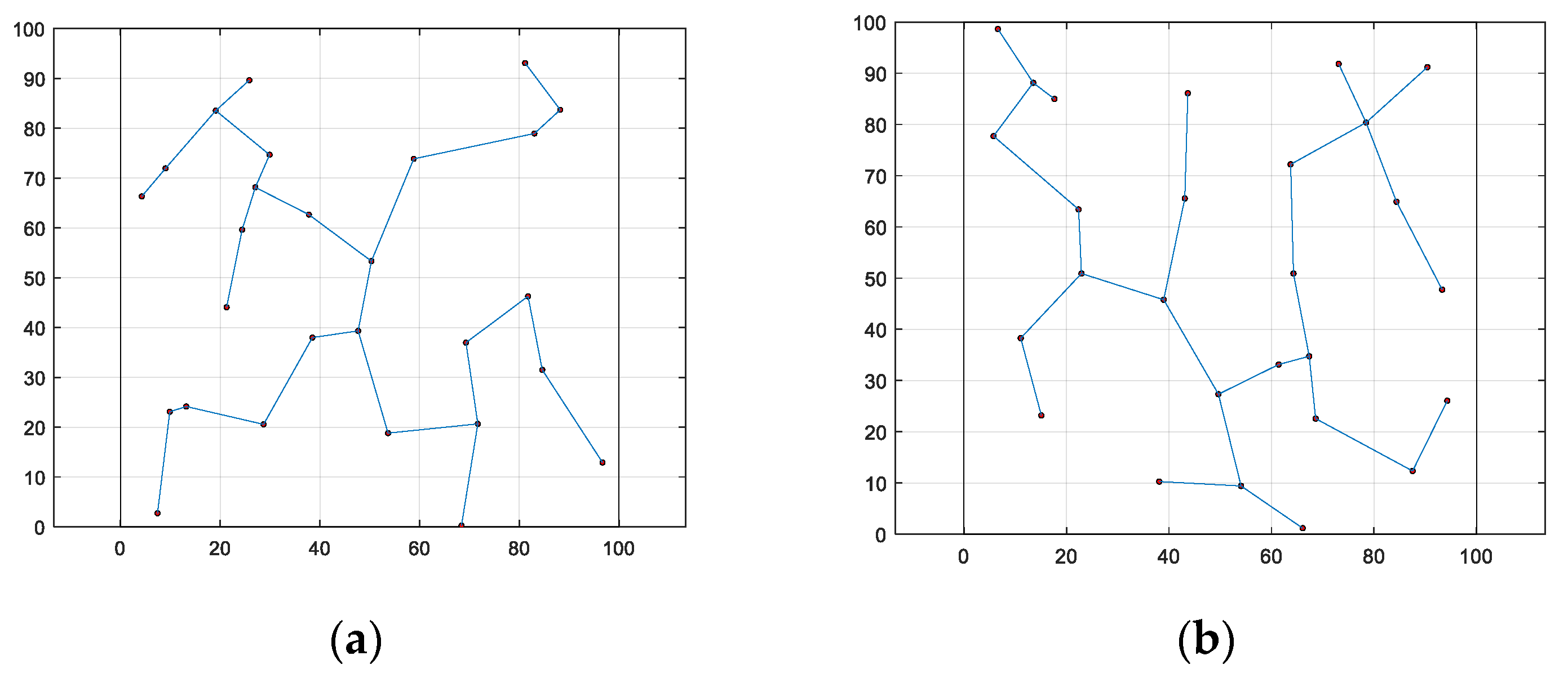
3.2. WOA-LFGA for WSN Coverage Optimization Problem

To verify the effectiveness of WOA-LFGA in the WSN coverage optimization problem, we compare the proposed algorithm with several other population intelligent algorithms and several other improved WOAs. Equations (4) and (5) are together used as the objective function when solving the WSN coverage optimization model. During the experiment, we found that WOA-LFGA was unable to manage its optimal performance in the coverage optimization problem of wireless sensors. After several experiments, we updated Formulas (21)–(23) for the coverage optimization problem of a wireless sensor:
X j t + 1 = c a n d i n d
where c a n d is a vector subject to rectangular distribution, its range is between (lb, ub + r), its dimension is (ublb + r)/r; r is the node radius of the wireless sensor; ind is the index coefficient, and its calculation formula is expressed as Formula (24):
i n d = j % r + 1                                                                                                                                     i f   j   i s   o d d c o s π j 2 j r % 2 + 1 + c o s π j 4 + 2 j 2 r         i f   j   i s   e v e n
where j is the dimension index of the whale individual, and % is the mod operator.
The aim of this experiment is to test and compare the improved WOA algorithm with the above five algorithms. The evaluation index is the average overall coverage rate and algorithm stability, which is represented by variance. We tested the coverage of 27 target points within an area of 100 m × 100 m, in which the coverage radius of each target point was 11 m. To make the experimental conclusions more persuasive, we conducted 30 experiments, with 200 iterations for each experiment. The parameter settings of the experiment are shown in Table 7.

3.2.1. Comparison of WOA-LFGA with Other Basic Algorithms

In this section, the effectiveness of WOA-LFGA is measured by comparing it with SMA [33], DOA [34], AOA, BWO [35], and WOA. The parameter settings of the comparison algorithm are all taken from the corresponding literature. In this experiment, the algorithm proposed in this paper is compared with the above five population intelligent algorithms, and the program operation results are shown in Table 8 and Figure 4.
It can be seen from Table 8 that, compared with SMA, DOA, AOA, BWO, and WOA, WOA-LFGA has significantly improved the coverage optimization of WSN. Overall, the optimization effect of SMA, AOA, and BWO in this experiment could be better, and the average coverage rate is below 70%. The other three algorithms have relatively high target point coverage and slight variance, which indicates that these algorithms play a role in the coverage optimization of wireless sensors. Specifically, the optimization results of WOA and DOA are similar, ranging from 75% to 80%, while the optimization effect of WOA is slightly higher, reaching 79.68%. However, the improved WOA in this paper achieves the current best optimization results, with a coverage rate of 90.97%, higher than the second place, 11.29% of the original WOA. WOA-LFGA has the lowest variance from the second evaluation index, and its value is 0.0019. That is, the algorithm has the highest stability. The improved WOA algorithm has certain advantages over the other five algorithms in terms of performance, combining the two evaluation indexes. From the perspective of coverage efficiency, WOA-LFGA also achieves the highest node coverage efficiency among the optimized algorithms, which fully demonstrates that the algorithm has lower node redundancy and a more even distribution of nodes in the area.
As seen in Figure 5, the WOA-LFGA proposed in this paper not only reaches the highest coverage rate but also has the fastest convergence rate. When the number of iterations reaches about 30% of the maximum number of iterations, it has reached the optimum. Although BWO is an excellent algorithm, its performance could be better for the problems proposed in this paper. The optimization effect of SMA and AOA is similar, and the coverage rate calculated by them hardly changes during the iteration process. Although the final coverage rate of WOA and DOA can reach nearly 80%, their convergence rate is slower than that of WOA-LFGA, and they need to iterate more than 60% to get close to the maximum coverage rate. The improved WOA in this paper is also superior to other algorithms in terms of convergence speed and has strong practicability and effectiveness in practical applications.
Using the sensor node configuration obtained from Figure 4, the Prim algorithm [36] was employed to generate a corresponding minimum spanning tree between the nodes, which was subsequently used to depict the communication network among the monitoring nodes, as presented in Figure 6.
From the perspective of communication distance uniformity and as observed in the results, the WOA-LFGA algorithm outperforms the other five compared algorithms. Moreover, the optimized communication network generated by the WOA-LFGA algorithm features more convergence nodes located near the edge, which is conducive to shortening the distance and saving energy consumption between the nodes during data transmission. Overall, in the process of node deployment, all six algorithms are capable of optimizing the placement of the nodes, thereby enhancing the coverage of the network. However, the network coverage optimized by the WOA-LFGA algorithm demonstrates the highest level of performance, with a more uniform distribution of the nodes. This contributes to improving the reliability of the overall network and reducing energy consumption during data transmission, thus extending the working time of the network.
By varying the number of sensor nodes N deployed in the above experiment, we investigate its impact on the network coverage. Specifically, we discuss the variation of network coverage with N ranging from 10 to 30 with a step size of 5. The experimental results are presented in Figure 7 and Table 9.
The figure clearly demonstrates the trend of network coverage variation with the change in the number of sensor nodes. Specifically, when the number of nodes is 20 or less, the difference in coverage between the different algorithms is not significant. However, it gradually becomes apparent after this threshold. From the graph, it is evident that WOA-LFGA can achieve a higher network coverage than the other algorithms with the same number of nodes. Furthermore, the curve indicates that WOA-LFGA has the fastest growth rate of coverage with the increasing number of nodes, demonstrating strong competitiveness compared to the other algorithms.

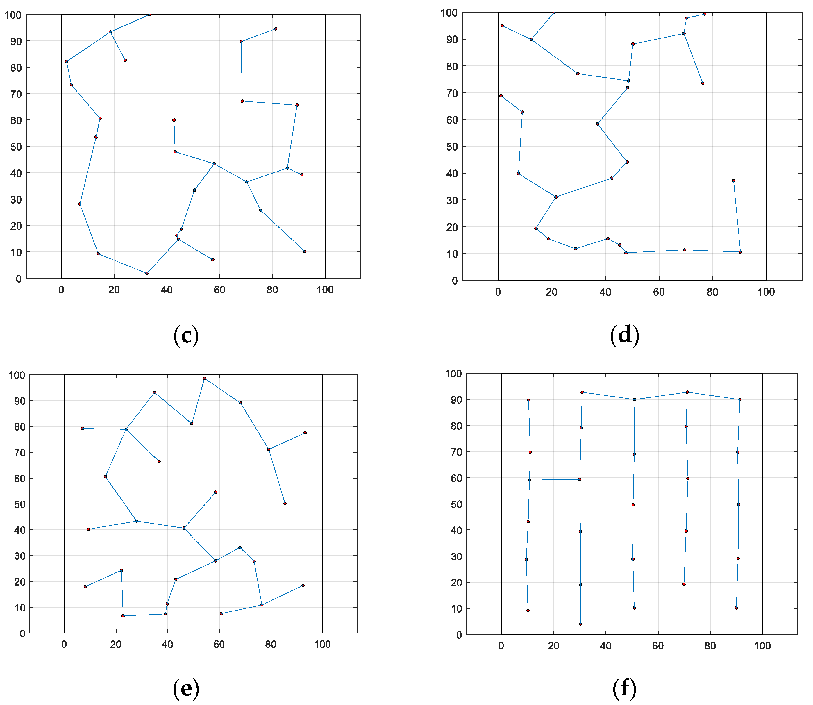
3.2.2. Comparison of WOA-LFGA with Different Modified WOA

In this subsection, the effectiveness of WOA-LFGA is measured by comparison with CWOA, WOABAT [37], RDWOA [38], WOAmM [39], EGE-WOA, where CWOA uses tent mapping. The parameter settings of the comparison algorithm are taken from the corresponding literature. In this experiment, the algorithm proposed in this paper is compared with the above five population intelligent algorithms, and the program operation results are shown in Table 10 and Figure 8.
It can be seen from Table 10 and Figure 9 that WOA-LFGA significantly improves the coverage optimization of WSN compared with CWOA, WOABAT, RDWOA, WOAmM, and EGE-WOA. In this experiment, the performance effect of EGE-WOA could be better. The coverage rate of EGE-WOA is below 60%, while that of CWOA is 68.34%, slightly higher than that of EGE-WOA. The coverage rate of WOA-BAT, RDWOA, and WOAmM reached an average of about 80%, or individual rates of 78.05%, 81.98%, and 81.24%, respectively. The average coverage rate of WOA-LFGA proposed in this paper is 90.97%, which achieves relatively adequate coverage and is 9% higher than the second place. WOA-LFGA has the lowest variance from the second evaluation index, and the algorithm stability is the best among several improved WOAs. Overall, WOA-LFGA has advantages over the other five algorithms’ overall performances.
Using the sensor node configuration obtained from Figure 8, the Prim algorithm was employed to generate a corresponding minimum spanning tree between the nodes, which was subsequently used to depict the communication network among the monitoring nodes, as presented in Figure 10.
From Figure 10, it is evident that WOA-LFGA still achieves more even communication distances compared with other optimized algorithms. This reduces the transmission power for information exchange, thus saving energy and extending the usage time of the entire network.
By varying the number of sensor nodes N deployed in the above experiment, we investigate its impact on the network coverage. Specifically, we discuss the variation of network coverage with N ranging from 10 to 30 with a step size of 5. The experimental results are presented in Figure 11 and Table 11.
Clearly, the following algorithms did not show much difference in optimization performance when the number of sensor nodes was less than 20. However, as the number exceeded 20, the advantage of WOA-LFGA gradually became apparent. With the same number of nodes, WOA-LFGA can better deploy wireless sensor nodes and maximize the coverage of the entire network. In terms of standard deviation, regardless of the number of sensor nodes, WOA-LFGA always has the smallest standard deviation, indicating that this algorithm has the best stability and the fastest growth rate. All these indicators together demonstrate the strong competitiveness of WOA-LFGA.

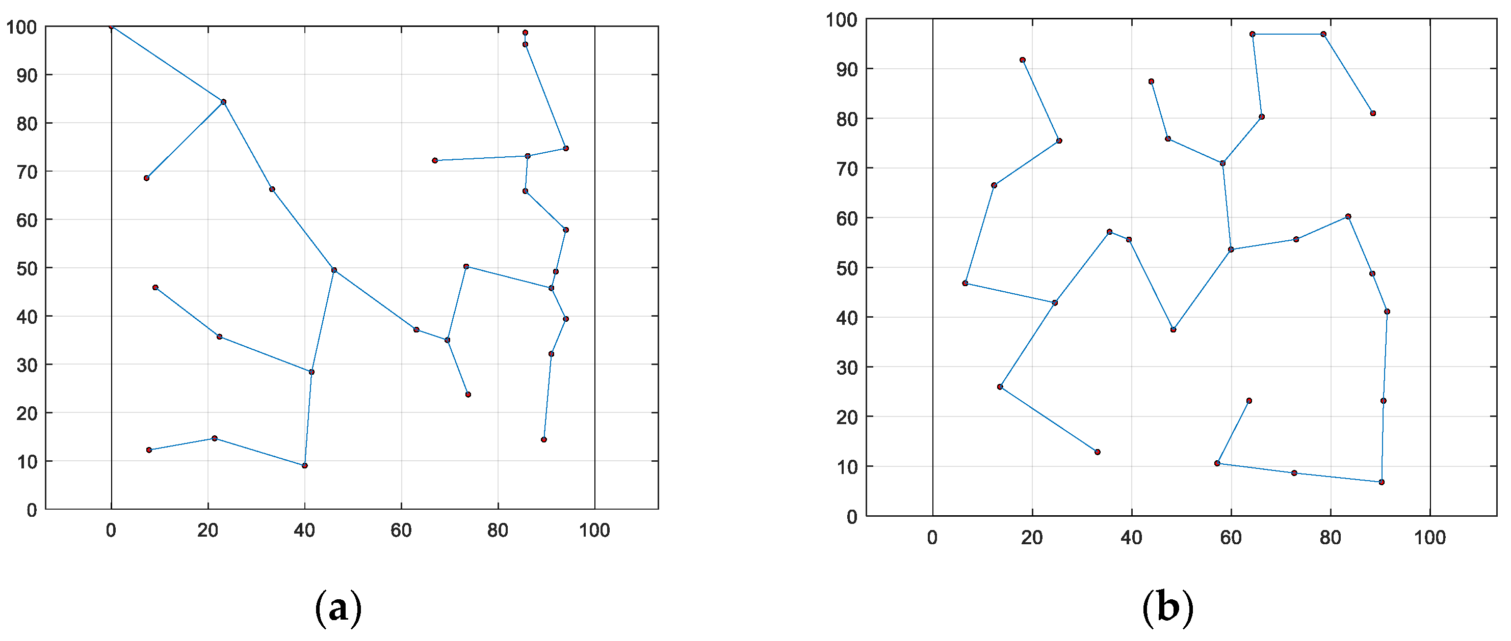
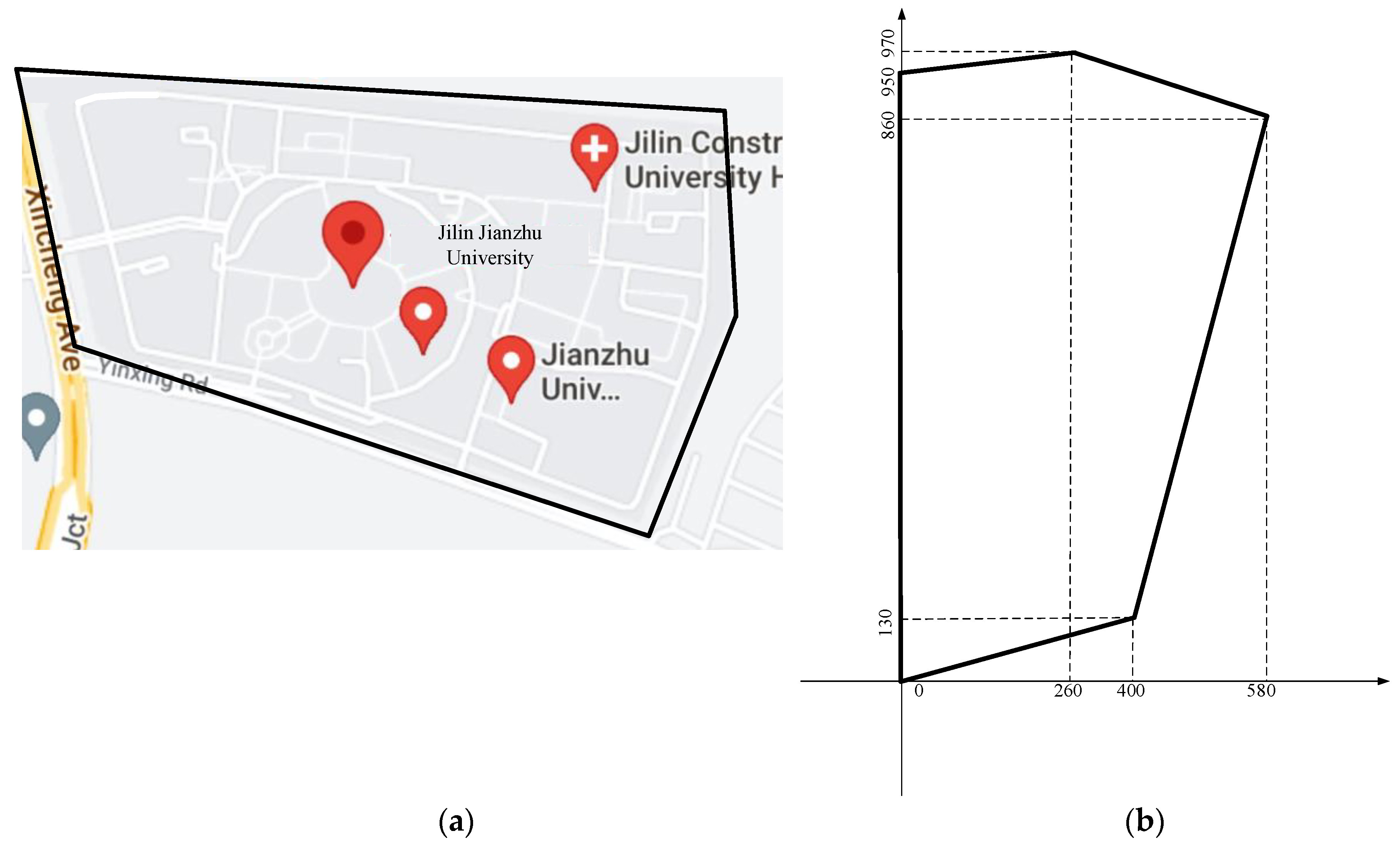
3.3. WOA-LFGA for WSN Coverage Practical Application

With the unprecedented development of big data, the widespread adoption of the fifth-generation mobile communication technology (5G) has accelerated. Currently, telecommunications operators worldwide are gradually rolling out 5G networks, and the development and application prospects of 5G technology are extremely promising. It can support a larger number of device connections and can contribute to the development of the Internet of Things (IoT) and the construction of smart cities. In this section, we apply the wireless sensor coverage optimization problem to real-life scenarios. Taking Jilin Jianzhu University as an example, as shown in Figure 12a, its outline can be abstracted as an irregular pentagon. For the sake of convenience in calculations, we rotate the shape counterclockwise by 90 degrees, as depicted in Figure 12b.
Equation (25) imposes constraints on the new boundary range.
0.325 x < y < 0.077 x + 950 , 0 < x 260 0.325 x < y < 0.281 x + 1043.125 , 261 < x 400 4.167 x 1536.667 < y < 0.281 x + 1043.125 , 401 < x 580
In this experiment, we tested the coverage of 13 target points within the aforementioned pentagonal area, in which the coverage radius of each target point was 100 m. To ensure that the experimental conclusions are more persuasive, we conducted 30 experiments, with 200 iterations for each experiment. The parameter settings of the experiment are shown in Table 12.

3.3.1. Comparison of WOA-LFGA with Other Basic Algorithms

In this subsection, the effectiveness of WOA-LFGA is measured by comparison with SMA, DOA, AOA, BWO, and WOA. Parameter Settings of the comparison algorithm are all taken from the corresponding literature. In this experiment, the algorithm proposed in this paper is compared with the above five population intelligent algorithms, and the program operation results are shown in Table 13.
It can be seen from Table 13 that, compared with SMA, DOA, AOA, BWO, and WOA, WOA-LFGA has significantly improved the coverage optimization of the WSN. In comparison, DOA, AOA, and BWO demonstrate better optimization performance, achieving coverage rates of over 50%. Both SMA and WOA also provided feasible solutions for wireless sensor coverage in this experiment. These algorithms have proven their efficacy in practical applications. Specifically, AOA and BWO yield similar optimization results, with coverage rates around 52%. DOA yields slightly higher optimization results, surpassing 53% coverage. However, the improved WOA algorithm in this study achieved the best optimization results, with an average coverage rate of 83.77%, surpassing the second-ranked algorithm by 30.71%. This is mainly due to WOA-LFGA’s different boundary handling strategy and excellent global search capabilities. In terms of variance, WOA-LFGA has the lowest variance, with a value of 0.0035, indicating its good stability. In terms of coverage efficiency, WOA-LFGA also achieves the highest node coverage efficiency among all algorithms, demonstrating lower node redundancy and a more uniform distribution of nodes in the area. Considering these three evaluation indexes, the improved WOA algorithm has certain advantages over the other five algorithms in terms of performance.
As seen in Figure 13, the WOA-LFGA proposed in this paper not only reaches the highest coverage rate but also has the fastest convergence rate. During the iteration process, it remained in a state of growth. Specifically, the growth was rapid in the first 30% of the iterations, but then slowed. The optimization effects of DOA and AOA are similar, as they show minimal noticeable growth during the iteration process. BWO exhibits relatively rapid growth, but the results are not significantly different from DOA. SMA and WOA are also excellent algorithms, but their performance in this experiment was not very satisfactory. The improved WOA presented in this paper outperforms other algorithms in terms of convergence speed and accuracy and demonstrates strong practicality and effectiveness in practical applications.

3.3.2. Comparison of WOA-LFGA with Different Modified WOA

In this subsection, the effectiveness of WOA-LFGA is measured by comparison with CWOA, WOABAT, RDWOA, WOAmM, and EGE-WOA, where CWOA uses tent mapping. The parameter settings of the comparison algorithm are taken from the corresponding literature. In this experiment, the algorithm proposed in this paper is compared with the above five population intelligent algorithms, and the program operation results are shown in Table 14.
It can be seen from Table 14 and Figure 14 that WOA-LFGA significantly improves the coverage optimization of WSN compared with CWOA, WOABAT, RDWOA, WOAmM, and EGE-WOA. In this experiment, the average coverage obtained by different improved whale algorithms varies. Among them, the evaluation coverage of WOABAT and WOAmM is less than 40%, while the average coverage obtained by EGE-WOA is slightly higher, reaching nearly 44%. The coverage of CWOA and RDWOA can exceed 50%, while the average coverage of the WOA-LFGA proposed in this article can reach 83.77%, which is 30.37% higher than the second place. The variance of WOA-LFGA is the smallest among several algorithms, which fully demonstrates that the stability of the algorithm is better than other algorithms. WOA-LFGA also has the highest coverage efficiency, which fully proves that the algorithm has a lower node redundancy and a more uniform regional node distribution. In summary, WOA-LFGA outperforms other algorithms in practical applications.

4. Conclusions

As IoT technology continues to advance, the internet of everything is becoming a reality. The rapid development of 5G technology will push various industries towards greater intelligence and efficiency. Smart cities, transportation, healthcare, and classrooms are increasingly integrated into people’s lives. The widespread application of IoT relies heavily on the rapid development of wireless sensors, which requires the reasonable deployment of sensor nodes within the monitored space, enabling fewer nodes to achieve greater coverage. This paper reviews solutions from international scholars and their teams that have addressed the coverage optimization problem of wireless sensors and conducts in-depth research on WSN coverage optimization using swarm intelligence algorithms.
This paper proposes the WOA-LFGA based on Lévy flight and genetic optimization mechanisms to comprehensively improve the effectiveness of the whale optimization algorithm. The algorithm has been successfully applied to 35 benchmark test functions and wireless sensor coverage problems. Comparative analysis of experimental simulation results reveals that the WOA-LFGA exhibits excellent global and local search abilities. Tests with single-mode and multi-mode reference functions demonstrate significant improvements in the algorithm’s convergence speed and accuracy, and its stability and ability to escape local optima are highly competitive compared with other intelligent optimization algorithms. Moreover, when applied to WSN coverage optimization problems and compared with other intelligent optimization algorithms, WOA-LFGA yields better optimization results, substantially improving coverage, convergence, and algorithm stability. Based on the experimental results presented in this paper, WOA-LFGA demonstrates strong competitiveness in intelligent optimization. Its application to other practical problems will become a more critical research direction in the future.

Author Contributions

Conceptualization, Y.Z.; methodology, B.Z.; software, B.Z.; investigation, B.Z.; resources, Y.X.; data curation, Y.X.; writing—original draft preparation, Y.X.; writing—review and editing, Y.Z. All authors have read and agreed to the published version of the manuscript.

Funding

This work is supported by the fund of the Science and Technology Development Project of Jilin Province No. 20220203190SF and the fund of the education department of Jilin province No. JJKH20210257KJ.

Institutional Review Board Statement

Not applicable.

Data Availability Statement

Not applicable.

Conflicts of Interest

The authors declare no conflict of interest.

References

  1. Mukherjee, M.; Adhikary, I.; Mondal, S.; Mondal, A.K.; Pundir, M.; Chowdary, V. Vision of IoT: Applications, Challenges, and Opportunities with Dehradun Perspective. In Proceeding of International Conference on Intelligent Communication, Control and Devices; Advances in Intelligent Systems and Computing; Springer: Singapore, 2017. [Google Scholar]
  2. Da Xu, L.; He, W.; Li, S. Internet of Things in Industries: A Survey. IEEE Trans. Ind. Inform. 2014, 10, 2233–2243. [Google Scholar]
  3. Zhao, X.; Askari, H.; Chen, J. Nanogenerators for smart cities in the era of 5G and Internet of Things. Joule 2021, 5, 1391–1431. [Google Scholar] [CrossRef]
  4. Majid, M.; Habib, S.; Javed, A.R.; Rizwan, M.; Srivastava, G.; Gadekallu, T.R.; Lin, J.C.W. Applications of Wireless Sensor Networks and Internet of Things Frameworks in the Industry Revolution 4.0: A Systematic Literature Review. Sensors 2022, 22, 2087. [Google Scholar] [CrossRef] [PubMed]
  5. Rashid, B.; Rehmani, M.H. Applications of wireless sensor networks for urban areas: A survey. J. Netw. Comput. Appl. 2016, 60, 192–219. [Google Scholar] [CrossRef]
  6. Li, M.; Li, Z.; Vasilakos, A.V. A Survey on Topology Control in Wireless Sensor Networks: Taxonomy, Comparative Study, and Open Issues. Proc. IEEE 2013, 101, 2538–2557. [Google Scholar] [CrossRef]
  7. Yoon, Y.; Kim, Y.H. Maximizing the coverage of sensor deployments using a memetic algorithm and fast coverage estimation. IEEE Trans. Cybern. 2021, 52, 6531–6542. [Google Scholar] [CrossRef] [PubMed]
  8. Liu, C.; Du, H.T. K-Sweep coverage with mobile sensor nodes in wireless sensor networks. IEEE Internet Things J. 2021, 8, 13888–13899. [Google Scholar] [CrossRef]
  9. Wang, W.; Huang, H.; He, F.; Xiao, F.; Sha, C. An enhanced virtual force algorithm for diverse k-coverage deployment of 3d underwater wireless sensor networks. Sensors 2019, 19, 3496. [Google Scholar] [CrossRef] [PubMed] [Green Version]
  10. Paulswamy, S.L.; Roobert, A.A.; Hariharan, K. A novel coverage improved deployment strategy for wireless sensor network. Wirel. Pers. Commun. 2021, 124, 868–891. [Google Scholar] [CrossRef]
  11. Priyadarshi, R.; Gupta, B. 2-D coverage optimization in obstacle-based FOI in WSN using modified PSO. J. Supercomput. 2022, 79, 4847–4869. [Google Scholar] [CrossRef]
  12. Zhu, W.; Huang, C.L.; Yeh, W.C.; Jiang, Y.; Tan, S.Y. A Novel Bi-Tuning SSO Algorithm for Optimizing the Budget-Limited Sensing Coverage Problem in Wireless Sensor Networks. Appl. Sci. 2021, 11, 10197. [Google Scholar] [CrossRef]
  13. Nematzadeh, S.; Torkamanian-Afshar, M.; Seyyedabbasi, A.; Kiani, F. Maximizing coverage and maintaining connectivity in WSN and decentralized IoT: An efficient metaheuristic-based method for environment-aware node deployment. Neural Comput. Appl. 2022, 35, 611–641. [Google Scholar] [CrossRef]
  14. Dao, T.K.; Chu, S.C.; Nguyen, T.T.; Nguyen, T.D.; Nguyen, V.T. An Optimal WSN Node Coverage Based on Enhanced Archimedes Optimization Algorithm. Entropy 2022, 24, 1018. [Google Scholar] [CrossRef] [PubMed]
  15. ZainEldin, H.; Badawy, M.; Elhosseini, M.; Arafat, H.; Abraham, A. An improved dynamic deployment technique based-on genetic algorithm (IDDT-GA) for maximizing coverage in wireless sensor networks. J. Ambient. Intell. Humaniz. Comput. 2020, 11, 4177–4194. [Google Scholar] [CrossRef]
  16. Mirjalili, S.; Lewis, A.D. The Whale Optimization Algorithm. Adv. Eng. Softw. 2016, 95, 51–67. [Google Scholar] [CrossRef]
  17. Zhang, J.; Wang, J.S. Improved Whale Optimization Algorithm Based On Nonlinear Adaptive Weight and Golden Sine Operator. IEEE Access 2020, 8, 77013–77048. [Google Scholar] [CrossRef]
  18. Liu, J.; Shi, J.; Hao, F.; Dai, M. A novel enhanced global exploration whale optimization algorithm based on Lévy flights and judgment mechanism for global continuous optimization problems. Eng. Comput. 2022, 39, 2433–2461. [Google Scholar] [CrossRef]
  19. Kaur, G.; Arora, S. Chaotic whale optimization algorithm. J. Comput. Des. Eng. 2018, 5, 275–284. [Google Scholar] [CrossRef]
  20. Bozorgi, S.M.; Yazdani, S. IWOA: An improved whale optimization algorithm for optimization problems. J. Comput. Des. Eng. 2019, 6, 243–259. [Google Scholar]
  21. Luo, J.; Shi, B.Y. A hybrid whale optimization algorithm based on modified differential evolution for global optimization problems. Appl. Intell. 2019, 49, 1982–2000. [Google Scholar] [CrossRef]
  22. Mafarja, M.; Jaber, I.; Ahmed, S.; Thaher, T. Whale Optimisation Algorithm for high-dimensional small-instance feature selection. Int. J. Parallel Emergent Distrib. Syst. 2019, 32, 80–96. [Google Scholar] [CrossRef]
  23. Zhang, M.; Wu, Q.; Chen, H.; Heidari, A.A.; Cai, Z.; Li, J.; Abdelrahim, E.M.; Mansour, R.F. Whale Optimization with Random Contraction and Rosenbrock Method for COVID-19 disease prediction. Biomed. Signal Process. Control 2023, 83, 104638. [Google Scholar] [CrossRef] [PubMed]
  24. Shivahare, B.D.; Gupta, S.K. Efficient covid-19 ct scan image segmentation by automatic clustering algorithm. J. Healthc. Eng. 2022, 2022, 9009406. [Google Scholar] [CrossRef] [PubMed]
  25. Tong, W. A hybrid algorithm framework with learning and complementary fusion features for whale optimization algorithm. Sci. Program. 2020, 2020, 5684939. [Google Scholar] [CrossRef] [Green Version]
  26. Prabhakar, D.; Satyanarayana, M. Side lobe pattern synthesis using hybrid sswoa algorithm for conformal antenna array. Eng. Sci. Technol. Int. J. 2019, 22, 1169–1174. [Google Scholar] [CrossRef]
  27. Mohammed, H.; Rashid, T. A novel hybrid GWO with WOA for global numerical optimization and solving pressure vessel design. Neural Comput. Appl. 2020, 32, 14701–14718. [Google Scholar] [CrossRef] [Green Version]
  28. Mantegna, R.N. Fast, accurate algorithm for numerical simulation of Lévy stable stochastic processes. Phys. Rev. E 1994, 49, 4677–4683. [Google Scholar] [CrossRef] [PubMed]
  29. Kennedy, J.; Eberhart, R.C. Particle swarm optimization. In Proceedings of the ICNN’95—International Conference on Neural Networks, Perth, WA, Australia, 27 November–1 December 1995; pp. 1942–1948. [Google Scholar]
  30. Abualigah, L.; Diabat, A.; Mirjalili, S.; Abd Elaziz, M.; Gandomi, A.H. The Arithmetic Optimization Algorithm. Comput. Methods Appl. Mech. Eng. 2021, 376, 113609. [Google Scholar] [CrossRef]
  31. Mirjalili, S.; Mirjalili, S.M.; Lewis, A. Grey Wolf Optimizer. Adv. Eng. Softw. 2014, 69, 46–61. [Google Scholar] [CrossRef] [Green Version]
  32. Mirjalili, S.; Gandomi, A.H.; Mirjalili, S.Z.; Saremi, S.; Faris, H.; Mirjalili, S.M. Salp swarm algorithm: A bio-inspired optimizer for engineering design problems. Adv. Eng. Softw. 2017, 114, 163–191. [Google Scholar] [CrossRef]
  33. Li, S.; Chen, H.; Wang, M.; Heidari, A.A.; Mirjalili, S. Slime mould algorithm: A new method for stochastic optimization. Future Gener. Comput. Syst. 2020, 111, 300–323. [Google Scholar] [CrossRef]
  34. Peraza-Vázquez, H.; Peña-Delgado, A.F.; Echavarría-Castillo, G.; Morales-Cepeda, A.B.; Velasco-Álvarez, J.; Ruiz-Perez, F. A Bio-Inspired Method for Engineering Design Optimization Inspired by Dingoes Hunting Strategies. Math. Probl. Eng. 2021, 2021, 9107547. [Google Scholar] [CrossRef]
  35. Zhong, C.; Li, G.; Meng, Z. Beluga whale optimization: A novel nature-inspired metaheuristic algorithm. Knowl. Based Syst. 2022, 251, 109215. [Google Scholar] [CrossRef]
  36. Prim, R. Shortest connection networks and some generalizations. Bell Syst. Tech. J. 1957, 36, 1389–1401. [Google Scholar] [CrossRef]
  37. Mohammed, H.M.; Umar, S.U.; Rashid, T.A. A Systematic and Meta-Analysis Survey of Whale Optimization Algorithm. Comput. Intell. Neurosci. 2019, 2019, 8718571. [Google Scholar] [CrossRef] [PubMed] [Green Version]
  38. Mohammed, H.M.; Umar, S.U.; Rashid, T.A. An efficient double adaptive random spare reinforced whale optimization algorithm. Expert Syst. Appl. 2020, 154, 113018. [Google Scholar] [CrossRef]
  39. Chakraborty, S.; Saha, A.K.; Sharma, S.; Mirjalili, S.; Chakraborty, R. A novel enhanced whale optimization algorithm for global optimization. Comput. Ind. Eng. 2021, 153, 107086. [Google Scholar] [CrossRef]
Figure 1. The crossover strategy in the genetic algorithm.
Biomimetics 08 00354 g001
Figure 2. The curve characteristics of Equation (21).
Biomimetics 08 00354 g002
Figure 3. Comparison of convergence curves of WOA-LFGA and other algorithms obtained in some of the benchmark problems.
Biomimetics 08 00354 g003aBiomimetics 08 00354 g003b
Figure 4. Node coverage distribution diagram. (a) SMA, (b) DOA, (c) AOA, (d) BWO, (e) WOA, (f) WOA-LFGA.
Biomimetics 08 00354 g004
Figure 5. Comparison of convergence curves of WOA-LFGA and other basic algorithms obtained in WSN coverage optimization problem.
Biomimetics 08 00354 g005
Figure 6. The composition of sensor nodes. (a) SMA, (b) DOA, (c) AOA, (d) BWO, (e) WOA, (f) WOA-LFGA.
Biomimetics 08 00354 g006aBiomimetics 08 00354 g006b
Figure 7. The impact of the number of sensor nodes on the network coverage between WOA-LFGA and other basic algorithms.
Biomimetics 08 00354 g007
Figure 8. Node coverage distribution diagram. (a) CWOA, (b) WOABAT, (c) RDWOA, (d) WOAmM, (e) EGE-WOA, (f) WOA-LFGA.
Biomimetics 08 00354 g008
Figure 9. Comparison of convergence curves of WOA-LFGA and different modified WOA obtained in WSN coverage optimization problem.
Biomimetics 08 00354 g009
Figure 10. The composition of sensor nodes. (a) CWOA, (b) WOABAT, (c) RDWOA, (d) WOAmM, (e) EGE-WOA, (f) WOA-LFGA.
Biomimetics 08 00354 g010aBiomimetics 08 00354 g010b
Figure 11. The impact of the number of sensor nodes on the network coverage between WOA-LFGA and different modified WOA.
Biomimetics 08 00354 g011
Figure 12. Jilin Jianzhu University. (a) Map of Jilin Jianzhu University, (b) Abstract of the Outline of Jilin Jianzhu University.
Biomimetics 08 00354 g012
Figure 13. Comparison of convergence curves of WOA-LFGA and other basic algorithms obtained in WSN coverage practical application.
Biomimetics 08 00354 g013
Figure 14. Comparison of convergence curves of WOA-LFGA and different modified WOA obtained in WSN coverage practical application.
Biomimetics 08 00354 g014aBiomimetics 08 00354 g014b
Table 1. Description of unimodal benchmark functions.
FunctionDRangefmin
F 1 x = i = 1 D x i 2 30[−100, 100]0
F 2 x = i = 1 D x i + i = 1 D x i 30[−10, 10]0
F 3 x = i = 1 D j 1 i x j 2 30[−100, 100]0
F 4 x = m a x i { | x i | , 1 i D } 30[−100, 100]0
F 5 x = i = 1 D 1 100 x i + 1 x i 2 2 + x i 1 2 30[−30, 30]0
F 6 x = i = 1 D x i + 0.5 2 30[−100, 100]0
F 7 x = i = 1 D i x i 4 + r a n d o m 0 ,   1 30[−1.28, 1.28]0
F 8 x = i = 1 D x i i + 1 30[−1, 1]0
F 9 x = i = 1 D j = 1 D x j 2 30[−100, 100]0
F 10 x = i = 1 D x i 2 + i = 1 D 0.5 i x i 2 + i = 1 D 0.5 i x i 4 30[−5, 10]0
Table 2. Description of multimodal benchmark functions.
FunctionDRangefmin
F 11 ( x ) = i = 1 D x i s i n ( | x i | ) 30[−500, 500]−418.98 × D
F 12 ( x ) = 1 + i = 1 D s i n 2 ( x i ) exp ( i = 1 D x i 2 ) 30[−10, 10]0
F 13 ( x ) = 0.5 i = 1 D ( x i 4 16 x i 2 + 5 x i ) 30[−5, 5]−39.166 × D
F 14 ( x ) = i = 1 D [ x i 2 10   c o s ( 2 π x i ) + 10 ] 30[−5.12, 5.12]0
F 15 ( x ) = 20 e x p ( 0.2 1 n i = 1 D x i 2 ) e x p ( 1 n i = 1 D cos ( 2 π x i ) ) + 20 + e 30[−32, 32]0
F 16 ( x ) = 1 4000 i = 1 D x i 2 i = 1 D c o s ( x i i ) + 1 30[−600, 600]0
F 17 ( x ) = ( i = 1 D s i n 2 ( x i ) e x p ( i = 1 D x i 2 ) ) e x p ( i = 1 D s i n 2 | x i | ) 30[−10, 10]−1
F 18 ( x ) = π D { 10 sin ( π y 1 ) + i = 1 D 1 ( y i 1 ) 2 [ 1 + 10 sin 2 ( π y i + 1 ) ]                                   + ( y n 1 ) 2 } + i = 1 D u ( x i ,   10 ,   100 ,   4 ) 30[−50, 50]0
F 19 ( x ) = 0.1 { sin 2 ( 3 π x 1 ) + i = 1 D ( x i 1 ) 2 [ 1 + sin 2 ( 3 π x i + 1 ) ]
+ ( x n 1 ) 2 [ 1 + s i n 2 ( 2 π x D ) ] } + i = 1 D u ( x i ,   5 ,   100 ,   4 )
30[−50, 50]0
F 20 ( x ) = ( 1 500 + j = 1 25 1 j + i = 1 2 ( x i a i j ) 6 ) 1 2[−65, 65]1
F 21 ( x ) = i = 1 11 [ a i x 1 ( b i 2 + b i x 2 ) b i 2 + b i x 3 + x 4 ] 2 4[−5, 5]0.00030
F 22 ( x ) = 4 x 1 2 2.1 x 1 4 + 1 3 x 1 6 + x 1 x 2 4 x 2 2 + 4 x 2 4 2[−5, 5]−10.316
F 23 ( x ) = ( x 2 5.1 4 π 2 x 1 2 + 5 π x 1 6 ) 2 + 10 ( 1 1 8 π ) cos x 1 + 10 2[−5, 5]0.398
F 24 ( x ) = [ 1 + ( x 1 + x 2 + 1 ) 2 ( 19 14 x 1 + 3 x 1 2 14 x 2
+ 6 x 1 x 2 + 3 x 2 2 ) ]   × [ 30 + ( 2 x 1 3 x 2 ) 2
× ( 18 32 x 1 + 12 x 1 2 + 48 x 2 36 x 1 x 2 + 27 x 2 2 ) ]
2[−2, 2]−3
F 25 ( x ) = i = 1 4 c i e x p ( j = 1 3 a i j ( x j p i j ) 2 ) 3[1, 3]−3.86
F 26 ( x ) = i = 1 4 c i e x p ( j = 1 6 a i j ( x j p i j ) 2 ) 6[0, 1]−3.32
F 27 ( x ) = i = 1 5 [ ( X a i ) ( X a i ) T + c i ] 1 4[0, 10]−10.1532
F 28 ( x ) = i = 1 7 [ ( X a i ) ( X a i ) T + c i ] 1 4[0, 10]−10.4028
F 29 ( x ) = i = 1 10 [ ( X a i ) ( X a i ) T + c i ] 1 4[0, 10]−10.5363
Table 3. Description of composite benchmark functions.
FunctionDRangefmin
F30(CF1): f1, f2, f3,…, f10 = Sphere Function
   [σ1, σ2, σ3,…, σ10] = [1, 1, 1,…, 1]
   [λ1, λ2, λ3,…, λ10] = [5/100, 5/100, 5/100,…, 5/100]
10[−5, 5]0
F31(CF2): f1, f2, f3,…, f10 = Griewank’s Function
   [σ1, σ2, σ3,…, σ10] = [1, 1, 1,…, 1]
   [λ1, λ2, λ3,…, λ10] = [5/100, 5/100, 5/100,…, 5/100]
10[−5, 5]0
F32(CF3): f1, f2, f3,…, f10 = Griewank’s Function
   [σ1, σ2, σ3,…, σ10] = [1, 1, 1,…, 1]
   [λ1, λ2, λ3,…, λ10] = [1, 1, 1,…, 1]
10[−5, 5]0
F33(CF4): f1, f2 = Ackley’s Function, f3, f4 = Rastrigin’s Function,
f5, f6 = Weierstrass Function, f7, f8 = Griewank’s Function,
f9, f10 = Sphere’s Function
   [σ1, σ2, σ3,…, σ10] = [1, 1, 1,…, 1]
   [λ1, λ2, λ3,…, λ10] = [5/32, 5/32, 1, 1, 5/0.5, 5/0.5, 5/100, 5/100, 5/100, 5/100]
10[−5, 5]0
F34(CF5): f1, f2 = Rastrigin’s Function, f3, f4 = Weierstrass Function, f5, f6 = Griewank’s Function, f7, f8 = Ackley’s Function,
f9, f10 = Sphere’s Function
   [σ1, σ2, σ3,…, σ10] = [1, 1, 1,…, 1]
   [λ1, λ2, λ3,…, λ10] = [1/5, 1/5, 5/0.5, 5/0.5, 5/100, 5/100, 5/32, 5/32, 5/100, 5/100]
10[−5, 5]0
F35(CF6): f1, f2 = Rastrigin’s Function, f3, f4 = Weierstrass Function, f5, f6 = Griewank’s Function, f7, f8 = Ackley’s Function,
f9, f10 = Sphere’s Function
   [σ1, σ2, σ3,…, σ10] = [0.1, 0.2, 0.3, 0.4, 0.5, 0.6, 0.7, 0.8, 0.9, 1]
   [λ1, λ2, λ3,…, λ10] = [0.1 × 1/5, 0.2 × 1/5, 0.3 × 5/0.5, 0.4 × 5/0.5, 0.5 × 5/100, 0.6 × 5/100, 0.7 × 5/32, 0.8 × 5/32, 0.9 × 5/100, 1 × 5/100]
10[−5, 5]0
Table 4. Comparison of optimization results obtained for the unimodal and multimodal benchmark functions.
PSOAOAGWOSSAWOAWOA-LFGA
avestdavestdavestdavestdavestdavestd
F10.011450.0162141.82 × 10−209.99 × 10−202.71 × 10−277.04 × 10−271.42 × 10−071.62 × 10−072.31 × 10−711.14 × 10−7000
F22.0205434.065539001.08 × 10−168.93 × 10−172.2853711.6668591.07 × 10−504.58 × 10−5000
F32444.1181926.8350.0036590.0074019.85 × 10−061.90 × 10−051382.524777.852571.50822172.512200
F47.0363861.3114990.0259430.0197518.16 × 10−078.64 × 10−0711.600463.6037771.2932071.2175861.65 × 10−107.94 × 10⁻¹⁰
F5237.9364552.16828.430770.24182527.09960.744425358.5001543.552427.723180.38172520.7728510.26487
F60.0086980.0144063.189660.2525490.7670480.3937042.80 × 10−075.94 E−070.2630310.1993830.0709580.122792
F70.0496370.0172756.93 × 10−056.73 E−050.0016630.00080.1908370.0752920.0030310.0027590.0017480.003825
F81.62 × 10−187.45 × 10−18001.60 × 10−948.74 × 10−941.60 × 10−061.04 × 10−068.07 × 10−1014.42 × 10−10000
F93715.1673804.0740.0063060.0151881.00 × 10−051.44 × 10−051543.173827.1876139.0415349.05663.84 × 10−261.99 × 10⁻²⁵
F10135.174986.41104278.75450.120353.35 × 10−077.80 × 10−0743.3259315.7774125.84223104.5636.12 × 10−173.35 × 10⁻¹⁶
F11−8588.58743.6667−5347.08428.9775−5856.44736.0021−7429.88767.0725−10327.81815.032−62304.42.22 × 10−11
F121.858340.705254002.086912.00149411.48 × 10−090.1290030.40765900
F13−1010.5332.04003−488.89565.78818−906.16366.86702−999.6941.44037−1173.673.427174−1174.980.005266
F1454.1766812.63687001.9483713.15016847.8574615.997061.89 × 10−151.04 × 10−1400
F150.7686490.6686768.88 × 10−1601.03 × 10−131.69 × 10−142.4819780.9133834.20 × 10−152.46 × 10−158.88 × 10−160
F160.0356940.0425620.1826220.1312190.0046290.0084190.0159760.008760.010460.03982400
F177.94 × 10−154.29 × 10−147.38 × 10−086.46 × 10−081.19 × 10−153.31 × 10−162.39 × 10−161.31 × 10⁻¹⁵−14.61 × 10⁻¹⁷−10
F180.1707330.2763310.5216440.0517920.0545420.028576.8343282.627910.013980.0168930.0068350.019706
F190.1569880.1968882.8400980.0984640.6287010.1963513.6070114.963270.2782070.1850770.2080520.199385
F200.9980045.83 × 10−178.27964.8500093.6761163.8742221.2952930.8277862.8656042.9976161.6873281.873362
F210.0026260.0060210.0128790.0224590.0044510.0080950.0015580.0035630.0006120.0002970.0003620.000218
F22−1.031636.45 × 10−16−1.031631.30 × 10−07−1.031632.57 × 10−08−1.031632.67 × 10−14−1.031639.35 × 10−10−1.031634.91 × 10−16
F230.39788700.408930.0087380.3978892.69 × 10−060.3978873.68 × 10−140.3978918.11 × 10−060.3978876.37 × 10−15
F2431.24 × 10−156.601279.3346353.000056.62 × 10−0532.13 × 10−133.9001124.92950331.63 × 10−06
F25−3.862782.65 × 10−15−3.851960.004077−3.86150.00228−3.862781.89 × 10−11−3.857170.009316−3.862782.14 × 10−15
F26−3.265140.07867−3.069290.075255−3.256270.085463−3.218380.05356−3.258650.122607−3.286330.055417
F27−6.017143.525257−3.584491.100864−8.515352.579639−8.650392.831563−6.574412.361348−10.15323.51 × 10−14
F28−8.443323.329769−4.014151.838357−10.40140.000913−8.442123.093598−7.382452.669453−10.40292.28 × 10−13
F29−7.26283.864573−3.453131.352861−9.813222.238027−8.030923.636316−7.684582.925501−10.53641.29 × 10−12
Table 5. Comparison of optimization results obtained for the composite benchmark functions.
PSOAOAGWOSSAWOAWOA-LFGA
avestdavestdavestdavestdavestdavestd
F30188.4598104.2843429.9201122.6024165.2451120.3013143.3333138.1736147.113109.186981.9337109.8375
F31210.1492147.6265603.8082141.238217.9645110.3465193.744119.9475212.4452102.3541167.121119.973
F32254.4012118.5757739.0197169.9494218.669100.6576329.7179239.0358494.4398203.5997438.3484132.1945
F33497.786191.054853.328370.53408709.6582188.0356630.5518272.5582633.3295174.6679576.9929128.6628
F34249.408231.7561493.5288182.9644187.0822137.7849182.7982202.8263206.8386159.906165.38111.3664
F35826.5022155.8774877.269166.94098837.5018152.0384762.027185.1875824.9949159.4651814.3615167.8058
Table 6. Results of test functions (F1–F19) with 30, 50, 100 and 500 dimensions.
PSOAOAGWOSSAWOAWOA-LFGA
Davestdavestdavestdavestdavestdavestd
F15010.8634714.445370.0008630.0016396.16 × 10−204.36 × 10−200.855481.0037251.66 × 10−737.15 × 10−7300
1002316.1093668.9310.0216990.0085171.75 × 10−121.2 × 10−121471.517385.54543.39 × 10−721.51 × 10−7100
500235236.425977.070.63330.0373210.0014530.00052196418.895452.5271.71 × 10−735.04 × 10−7300
F25010.5308311.771912.3 × 10−1471 × 10−1462.51 × 10−121.32 × 10−128.8953752.8015842.35 × 10−491.05 × 10−4800
10065.3626322.837612.42 × 10−531.08 × 10−524.11 × 10−081.52 × 10−0848.256067.9483598.59 × 10−501.89 × 10−4900
5001390.407110.38610.0012320.0016680.0109380.00145541.612619.439793.87 × 10−491.68 × 10−4800
F35016884.774607.7520.1033860.0979210.3336690.5979599735.955803.166565.1298762.94053.86 × 10−191.73 × 10⁻¹⁸
100101956.411759.161.1274561.75346636.1386928.24776445132153.114706.5167708.6183.07 × 10−171.37 × 10⁻¹⁶
5002764988318150.233.6795416.67636334085.195550.541275053728370.788474.96146520.32.52 × 10−121.13 × 10⁻¹¹
F45017.962431.7076760.0467210.0159610.0002720.00020220.630424.2589612.1525912.3615062.43 × 10−101.07 × 10−09
10040.446953.3972690.0929030.0108750.5872540.43348427.994272.7441133.3880532.9588311.38 × 10−104.27 × 10⁻¹⁰
50076.607423.5873350.1807150.01315165.338155.51939740.294552.2920223.3800972.4109429.41 × 10−093.08 × 10−08
F5505662.01719968.4748.771040.15702947.436320.9473893276.495682.86848.047470.40316234.751320.54994
100203892.768214.3898.871630.11573797.962760.542074156566.475343.7398.138260.1911949.0368348.75961
5004.59 × 10+081.37 × 10+08499.09660.064668498.0830.237754375975203829547495.87580.415621161.4206225.6898
F6508.7623547.9645437.1482220.3825532.7631380.6039880.5948130.5906890.8386580.3621110.5287710.43255
1002473.4023667.76518.22890.6345610.57051.2296641426.96511.4862.2775570.8101512.2154891.824284
500229660.131072.21116.00741.08118792.015621.95832793586.056284.00819.578777.91201819.3064121.22633
F7500.5964021.8068437.14 × 10−055.37 × 10−050.0031660.0015270.5647580.1284040.0036140.0041850.0021360.003517
1006.5365458.8266386.06 × 10−055.39 × 10−050.0069480.0042532.8439640.6590530.0036860.0030960.0016280.004275
5003707.805687.69928.02 × 10−058.17 × 10−050.0490750.012875276.436953.533030.0032760.0046610.0009240.000913
F8501.44 × 10−143.85 × 10−14001.86 × 10−886.35 × 10−882.19 × 10−061.69 × 10−061.2 × 10−1075.5 × 10−10700
1002.64 × 10−118.42 × 10−11002.15 × 10−359.61 × 10−352.29 × 10−061.67 × 10−069.8 × 10−1042.8 × 10−10300
5001.88 × 10−054.2 × 10−05000.0002710.0011315.71 × 10−067.21 × 10−061.3 × 10−1105.7 × 10−11000
F95018886.555430.5190.056310.0494530.3671360.65784310379.315073.609711.41741668.8141.98 × 10−148.84 × 10⁻¹⁴
10010645015037.641.0590310.969092641.6541619.224143718.8725770.165269.8647375.0781.21 × 10−205.02 × 10⁻²⁰
500269674438583538.492728.86932328280.466473.191217109526500.8162555268337513.41 × 10−181.36 × 10⁻¹⁷
F1050624.1645207.4525798.670998.335660.0735480.07947391.207189.3828546.64148192.67380.0042310.018922
1002536.807451.222051.827173.7202122.667452.301591956.498227.5388227.8372676.57954.18 × 10−050.000187
50024484.751175.0668.84 ×10+143.54 ×10+153854.575356.618710441.52642.2583559.55881632.451500.78071714.189
F1150−12786.3798.5763−6730.6555.5429−9006.98796.4451−11829.81409.544−17237.63259.934−1038412.99 × 10−11
100−21997.31611.842−9932.03556.0954−16523.71163.17−22109.61951.76−330536993.32−2076815.97 × 10−11
500−65272.32572.758−22147.41418.863−53823.413825.98−60450.65024.125−18334428730.9910384071.19 × 10−10
F12503.5122781.823459001.9978520.7679041.005910.0098820000
1008.7088943.634477002.9695320.6499413.569480.8208590.0526190.23531800
500116.90729.1524896.35 × 10−061.81 × 10−0628.2037159.83419107.2744.1170315.55 × 10 −182.48 × 10 −1700
F1350−1681.4745.5754−675.22676.99906−1352.1590.40042−1648.1138.54963−1956.641.398103−1958.070.215703
100−3303.1963.15214−1084.03124.9054−2299.99157.4946−3023.5571.17438−3910.895.958551−3915.880.840303
500−12380.6261.834−3680.81261.3991−7753.78531.8809−10816.8224.6012−19540.234.90968−19567.537.75219
F1450119.936528.58934004.1789334.7496788.488630.733740000
100382.735554.843860010.742897.341498230.932735.079830000
5004449.093186.36695.97 × 10−065.37 × 10−0670.7617918.022813151.214160.97334.55 × 10−142.03 × 10−1300
F15502.7155870.4841158.88 × 10−1604.53 × 10−113.17 × 10−114.6350251.2062844.26 × 10−152.44 × 10−158.88 × 10−160
1006.5256482.0658370.0004840.0007931.22 × 10−074.02 × 10−0810.20931.0476674.26 × 10−152.7 × 10−158.88 × 10−160
50018.052840.4482870.0079140.0006620.0018760.00029314.249810.2240263.55 × 10−152.27 × 10−158.88 × 10−160
F16501.0592170.1455731.0622060.1444970.0034730.0076060.5081930.1779610.0086730.03878500
10035.2827850.71112585.2056187.62030.0034660.00847112.832642.8449185.55 × 10 −182.48 × 10 −1700
5002133.145209.971410516.472772.3510.0047280.020304867.91765.887220000
F17501.53 × 10−211.16 × 10−212.82 × 10−123.22 × 10−122.6 × 10−226.62 × 10−221.47 × 10−218.59 × 10⁻²²−16.24 × 10⁻¹⁷−10
1006.52 × 10−411.2 × 10−402.17 × 10−232.7 × 10−238.56 × 10−411.9 × 10−403.66 × 10−414.07 × 10−41−0.850.366348−10
5004.8 × 10−17701.3 × 10−1114.4 × 10−1111.1 × 10−17301.4 × 10−1820−0.70.470162−10
F18503.3868431.2287040.7341160.0447660.1068710.04738511.491352.7133140.0129430.0073240.0127620.020302
1002936.1186291.820.9012930.0254360.2767810.06077831.040310.66640.0202690.0111140.0167970.022049
5004.79 × 10+082.04 × 10+081.0821530.0109310.7669240.05827915303759266620.0246010.0116470.0444410.070781
F195042.5379620.413874.8752820.0807732.0852560.37357576.3641912.048960.4130980.2274860.3144420.409962
10073149.6162122.549.9682050.0578866.843290.4597639531.2615735.961.1390660.5844511.1348651.559223
5001.5 × 10+092.72 × 10+0850.2210.03900650.054961.39323403636192138937.2168213.1385014.8514146.68935
Table 7. Parameters of WSN coverage optimization problem in Section 3.2.
ParameterValue
Region size100 m × 100 m
Sensing range11 m
Sensor nodes number N27
Individual number50
Iterations200
Test times30
Table 8. Coverage ratio comparison of WOA-LFGA with other basic algorithms.
MethodavestdC
SMA68.9237%0.01730.6715
DOA76.2457%0.01830.7429
AOA68.3437%0.01370.6659
BWO64.1613%0.02050.6251
WOA79.6813%0.02310.7763
WOA-LFGA90.9703%0.00190.8863
Table 9. The variation of network coverage with different numbers of nodes between WOA-LFGA and other basic algorithms.
N = 10 N = 15 N = 20 N = 25 N = 30
Methodavestdavestdavestdavestdavestd
SMA34.63%0.0087747.70%0.0102857.51%0.0110266.70%0.0121573.96%0.02138
DOA37.73%0.0065753.55%0.0117664.77%0.0174373.12%0.0230579.83%0.01749
AOA34.59%0.0068547.58%0.0118357.85%0.018665.42%0.0142572.50%0.01506
BWO34.52%0.0091946.03%0.0163455.40%0.0225262.08%0.0200867.43%0.02664
WOA37.87%0.0026454.04%0.0137367.29%0.0178575.84%0.0253182.70%0.02263
WOA-LFGA38.29%0.0004256.72%0.0038172.16%0.0074788.75%0.0010593.71%0.00272
Table 10. Coverage ratio comparison of WOA-LFGA with different modified WOA.
MethodavestdC
CWOA68.3363%0.02630.6658
WOABAT78.0493%0.02170.7604
RDWOA81.9797%0.01710.7987
WOAmM81.2440%0.02500.7916
EGE-WOA56.2650%0.04890.5482
WOA-LFGA90.9703%0.00190.8863
Table 11. The variation of network coverage with different numbers of nodes between WOA-LFGA and different modified WOA.
N = 10 N = 15 N = 20 N = 25 N = 30
MethodavestdavestdavestdAvestdavestd
CWOA35.46%0.011648.44%0.022358.01%0.025365.02%0.018672.98%0.0251
WOABAT37.61%0.004053.81%0.010365.58%0.016074.49%0.023481.73%0.0210
RDWOA38.08%0.002155.11%0.007669.53%0.007878.40%0.015785.35%0.0236
WOAmM38.04%0.002054.93%0.010868.12%0.012078.04%0.020084.99%0.0214
EGE-WOA31.00%0.022141.04%0.044349.71%0.039151.94%0.053559.58%0.0627
WOA-LFGA38.29%0.000456.72%0.003872.16%0.007488.75%0.001093.71%0.0027
Table 12. Parameters of WSN coverage optimization problem in Section 3.3.
ParameterValue
Region size440,400 m2
Sensing range100 m
Sensor nodes number N13
Individual number50
Iterations200
Test times30
Table 13. Coverage ratio comparison of WOA-LFGA with other basic algorithms in practical application.
MethodavestdC
SMA11.4011%0.01590.1229
DOA53.0607%0.05300.5722
AOA52.3511%0.03060.5645
BWO52.2743%0.05790.5637
WOA37.2967%0.09350.4022
WOA-LFGA83.7718%0.00350.9033
Table 14. Coverage ratio comparison of WOA-LFGA with different modified WOA in practical application.
MethodavestdC
CWOA53.4095%0.06660.5759
WOABAT37.4971%0.05270.4043
RDWOA51.3324%0.05080.5535
WOAmM38.7471%0.04520.4178
EGE-WOA43.9632%0.03660.4741
WOA-LFGA83.7718%0.00350.9033
Disclaimer/Publisher’s Note: The statements, opinions and data contained in all publications are solely those of the individual author(s) and contributor(s) and not of MDPI and/or the editor(s). MDPI and/or the editor(s) disclaim responsibility for any injury to people or property resulting from any ideas, methods, instructions or products referred to in the content.

