
Research on Economic Optimal Dispatching of Microgrid Based on an Improved Bacteria Foraging Optimization

Abstract
:1. Introduction
- (1)
- This study improved the algorithm’s speed and considered its accuracy in chemotaxis. The adaptive step size formula replaces the standard fixed step size, and the PSO speed formula is introduced to improve the random direction vector (PHI).
- (2)
- The crisscross algorithm is used to improve the population of the algorithm and global search performance in the replication part.
- (3)
- The dynamic dispersal equation and sine-cosine algorithm were used to improve the loss of high-quality results and the algorithm’s efficiency for the dispersal part.
2. Microgrid Economic Dispatch Model
2.1. The Model of DG
2.2. Microgrid Economic Dispatching Model
3. An Improved Bacterial Foraging Optimization and Its Application
3.1. Chemotaxis Process
| Algorithm 1: Chemotaxis process with hybrid dynamic step size and PSO |
| 1 for j = 1:Nc |
| 2 for i = 1:s |
| 3 C = C(x) (C (x) represents the dynamic adaptive step size of the xth bacteria) |
| 4 Calculate the influence of bacterial clustering behavior on fitness value and save as Jl |
| 5 Replacing PHI with Particle Swarm Velocity Formula |
| 6 P(i,j + 1) = P(j) + C * PHI |
| 7 Update fitness value J |
| 8 while (m < Ns) |
| 9 if (J < Jl) |
| 10 Update fitness value J |
| 11 else |
| 12 m = Ns |
| 13 end |
| 14 end |
| 15 Update fitness value Jl |
| 16 end |
| 17 end |
3.2. Replication Process
| Algorithm 2: Replication Process of Hybrid CSO |
| 1 for k = 1:Nre |
| 2 for i = 0:s/2 − 1 |
| 3 if rand < Longitudinal crossing probability |
| 4 for j = 1:p |
| 5 Longitudinal crossing of populations |
| 6 end |
| 7 end |
| 8 end |
| 9 Update population according to fitness value |
| 10 for i = 0:p/2 − 1 |
| 11 for j = 1:s |
| 12 Horizontal crossing of populations |
| 13 end |
| 14 end |
| 15 end |
3.3. Dispersal Process
| Algorithm 3: Dispersion process of hybrid dynamic probability and SCA |
| 1 for l = 1:Ned |
| 2 for m = 1:s |
| 3 Dynamic dispersion probability |
| 4 if Ped > rand |
| 5 if r4 < 0.5 |
| 6 Sinusoidal oscillation search |
| 7 else |
| 8 Cosine oscillation search |
| 9 end |
| 10 end |
| 11 end |
| 12 end |
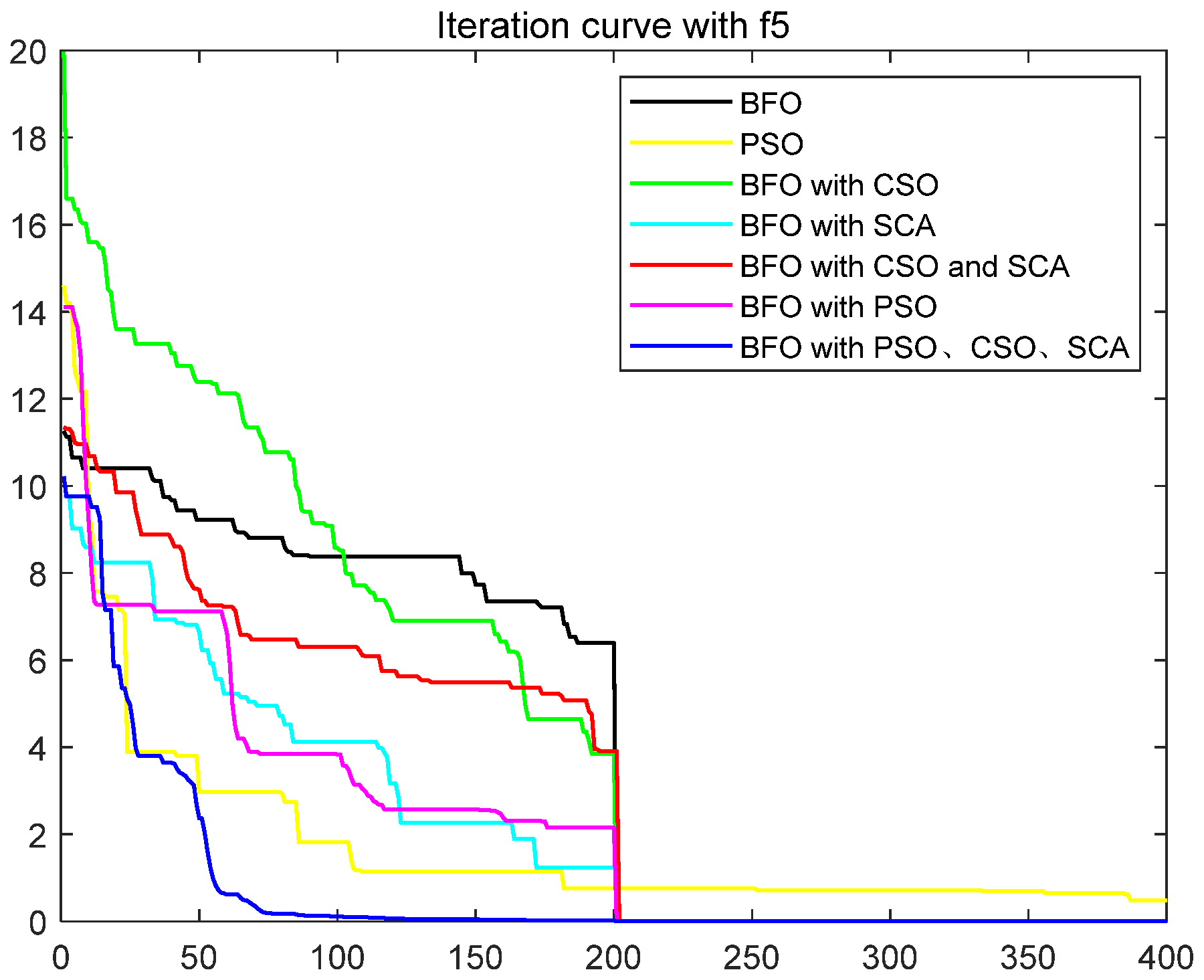
3.4. Test Analysis
4. Algorithm Application and Experimental Analysis
4.1. Uncertainty Treatment of Wind Power and Photovoltaic
4.2. Examples of Microgrid Dispatching
5. Conclusions
Author Contributions
Funding
Data Availability Statement
Conflicts of Interest
Abbreviations
| Name | Abbreviation |
| Particle Swarm Optimization | PSO |
| Genetic Algorithm | GA |
| Differential Evolution Algorithm | DE |
| Whale Optimization Algorithm | WOA |
| Bacterial Foraging Optimization | BFO |
| Sine-Cosine algorithm | SCA |
| Criss-cross Optimization | CSO |
| Distributed Generation | DG |
| PV power | PV |
| Power of Wind | PW |
| Number of chemotaxis restriction | Nc |
| Number of replication restriction | Nre |
| Number of dispersal restriction | Ned |
| Search Step Size | C |
| Probability of dispersion | Ped |
| Fitness value | J |
| Population | P |
References
- Sahoo, A.; Hota, P.K. Impact of energy storage system and distributed energy resources on bidding strategy of micro-grid in deregulated environment. J. Energy Storage 2021, 43, 103230. [Google Scholar] [CrossRef]
- Meng, A.; Xu, X.; Zhang, Z.; Zeng, C.; Liang, R.; Zhang, Z.; Wang, X.; Yan, B.; Yin, H.; Luo, J. Solving high-dimensional multi-area economic dispatch problem by decoupled distributed crisscross optimization algorithm with population cross generation strategy. Energy 2022, 258, 124836. [Google Scholar] [CrossRef]
- Das, A.; Wu, D.; Ni, Z. Approximate dynamic programming with policy-based exploration for microgrid dispatch under uncertainties. Int. J. Electr. Power Energy Syst. 2022, 142, 108359. [Google Scholar] [CrossRef]
- Sigalo, M.B.; Pillai, A.C.; Das, S.; Abusara, M. An Energy Management System for the Control of Battery Storage in a Grid-Connected Microgrid Using Mixed Integer Linear Programming. Energies 2021, 14, 6212. [Google Scholar] [CrossRef]
- Li, B.; Roche, R. Real-Time Dispatching Performance Improvement of Multiple Multi-Energy Supply Microgrids Using Neural Network Based Approximate Dynamic Programming. Front. Electron. 2021, 2, 637736. [Google Scholar] [CrossRef]
- Capuno, M.; Song, H. DC Microgrid Optimal Power Flow Using Nonlinear Programming. Proc. Acad. Conf. Korean Electr. Soc. 2016, 11, 68–69. [Google Scholar]
- Zheng, C.; Eskandari, M.; Li, M.; Sun, Z. GA−Reinforced Deep Neural Network for Net Electric Load Forecasting in Microgrids with Renewable Energy Resources for Scheduling Battery Energy Storage Systems. Algorithms 2022, 15, 338. [Google Scholar] [CrossRef]
- Dou, C.; Zhou, X.; Zhang, T.; Xu, S. Economic Optimization Dispatching Strategy of Microgrid for Promoting Photoelectric Consumption Considering Cogeneration and Demand Response. J. Mod. Power Syst. Clean Energy 2020, 8, 557–563. [Google Scholar] [CrossRef]
- Jiang, H.; Ning, S.; Ge, Q.; Yun, W.; Xu, J.; Bin, Y. Optimal economic dispatching of multi-microgrids by an improved genetic algorithm. IET Cyber-Syst. Robot. 2021, 3, 68–76. [Google Scholar] [CrossRef]
- Hernández-Ocaña, B.; García-López, A.; Hernández-Torruco, J.; Chávez-Bosquez, O. Bacterial Foraging Based Algorithm Front-end to Solve Global Optimization Problems. Intell. Autom. Soft Comput. 2022, 32, 1797–1813. [Google Scholar] [CrossRef]
- Hernández-Ocaña, B.; Hernández-Torruco, J.; Chávez-Bosquez, O.; Calva-Yáñez, M.B.; Portilla-Flores, E.A. Bacterial Foraging-Based Algorithm for Optimizing the Power Generation of an Isolated Microgrid. Appl. Sci. 2019, 9, 1261. [Google Scholar] [CrossRef] [Green Version]
- Awad, H.; Hafez, A. Optimal operation of under-frequency load shedding relays by hybrid optimization of particle swarm and bacterial foraging algorithms. Alex. Eng. J. 2022, 61, 763–774. [Google Scholar] [CrossRef]
- Jiang, J.; Zhou, R.; Xu, H.; Wang, H.; Wu, P.; Wang, Z.; Li, J. Optimal sizing, operation strategy and case study of a grid-connected solid oxide fuel cell microgrid. Appl. Energy 2022, 307, 118214. [Google Scholar] [CrossRef]
- Wang, J.; Liu, C.; Zhou, M. Improved Bacterial Foraging Algorithm for Cell Formation and Product Scheduling Considering Learning and Forgetting Factors in Cellular Manufacturing Systems. IEEE Syst. J. 2020, 14, 3047–3056. [Google Scholar] [CrossRef]
- Jalilpoor, K.; Nikkhah, S.; Sepasian, M.S.; Aliabadi, M.G. Application of precautionary and corrective energy management strategies in improving networked microgrids resilience: A two-stage linear programming. Electr. Power Syst. Res. 2022, 204, 107704. [Google Scholar] [CrossRef]
- Bio Gassi, K.; Baysal, M. Analysis of a linear programming-based decision-making model for microgrid energy management systems with renewable sources. Int. J. Energy Res. 2022, 46, 7495–7518. [Google Scholar] [CrossRef]
- Khalid, A.; Javaid, N.; Mateen, A.; Khalid, B.; Khan, Z.A.; Qasim, U. Demand Side Management Using Hybrid Bacterial Foraging and Genetic Algorithm Optimization Techniques. In Proceedings of the 2016 10th International Conference on Complex, Intelligent, and Software Intensive Systems (CISIS), Fukuoka, Japan, 6–8 July 2016; IEEE: New York, NY, USA, 2016. [Google Scholar]
- Liu, L.; Shan, L.; Dai, Y.; Liu, C.; Qi, Z. A Modified Quantum Bacterial Foraging Algorithm for Parameters Identification of Fractional-Order System. IEEE Access 2018, 6, 6610–6619. [Google Scholar] [CrossRef]
- Meng, A.; Ge, J.; Yin, H.; Chen, S. Wind speed forecasting based on wavelet packet decomposition and artificial neural networks trained by crisscross optimization algorithm. Energy Convers. Manag. 2016, 114, 75–88. [Google Scholar] [CrossRef]
- Zhang, M.; Xu, W.; Zhao, W. Combined optimal dispatching of wind-light-fire-storage considering electricity price response and uncertainty of wind and photovoltaic power. Energy Rep. 2023, 9, 790–798. [Google Scholar] [CrossRef]
- Yin, M.; Li, K.; Yu, J. A data-driven approach for microgrid distributed generation planning under uncertainties. Appl. Energy 2022, 309, 118429. [Google Scholar] [CrossRef]
- Mirjalili, S. SCA: A Sine Cosine Algorithm for solving optimization problems. Knowl.-Based Syst. 2016, 96, 120–133. [Google Scholar] [CrossRef]
- Mohammad, S.; Nasir, A.N.K.; Ghani, N.M.A.; Ismail, R.M.T.R.; Abd Razak, A.A.; Jusof, M.F.M.; Rizal, N.A.M. Hybrid Bacterial Foraging Sine Cosine Algorithm for Solving Global Optimization Problems. IOP Conf. Ser. Mater. Sci. Eng. 2020, 917, 12081. [Google Scholar] [CrossRef]
- Ni, N.; Zhu, Y. Self-adaptive bacterial foraging algorithm based on estimation of distribution. J. Intell. Fuzzy Syst. 2021, 40, 5595–5607. [Google Scholar] [CrossRef]
- Alhasnawi, B.N.; Jasim, B.H.; Siano, P.; Alhelou, H.H.; Al-Hinai, A. A Novel Solution for Day-Ahead Scheduling Problems Using the IoT-Based Bald Eagle Search Optimization Algorithm. Inventions 2022, 7, 48. [Google Scholar] [CrossRef]
- Alhasnawi, B.N.; Jasim, B.H.; Mansoor, R.; Alhasnawi, A.N.; Rahman, Z.A.S.A.; Haes Alhelou, H.; Guerrero, J.M.; Dakhil, A.M.; Siano, P. A new Internet of Things based optimization scheme of residential demand side management system. IET Renew. Power Gener. 2022, 16, 1992–2006. [Google Scholar] [CrossRef]
- Rezaei, N.; Meyabadi, A.F.; Deihimi, M. A game theory based demand-side management in a smart microgrid considering price-responsive loads via a twofold sustainable energy justice portfolio. Sustain. Energy Technol. Assess 2022, 52, 102273. [Google Scholar] [CrossRef]
- Kasruddin Nasir, A.N.; Ahmad, M.A.; Tokhi, M.O. Hybrid spiral-bacterial foraging algorithm for a fuzzy control design of a flexible manipulator. J. Low Freq. Noise Vib. Act. Control 2022, 41, 340–358. [Google Scholar] [CrossRef]
- Ping, L.; Xiangrui, K.; Chen, F.; Zheng, Y. Novel distributed state estimation method for the AC-DC hybrid microgrid based on the Lagrangian relaxation method. J. Eng. 2019, 2019, 4932–4936. [Google Scholar] [CrossRef]
- Behnamfar, M.R.; Barati, H.; Karami, M. Stochastic Multi-objective Short-term Hydro-thermal Self-scheduling in Joint Energy and Reserve Markets Considering Wind-Photovoltaic Uncertainty and Small Hydro Units. J. Electr. Eng. Technol. 2021, 16, 1327–1347. [Google Scholar] [CrossRef]
- Mao, W.; Dai, N.; Li, H. Economic dispatch of microgrid considering fuzzy control based storage battery charging and discharging. J. Electr. Syst. 2019, 15, 417–428. [Google Scholar]
- Du, X.; Wang, L.; Zhao, J.; He, Y.; Sun, K. Power Dispatching of Multi-Microgrid Based on Improved CS Aiming at Economic Optimization on Source-Network-Load-Storage. Electronics 2022, 11, 2742. [Google Scholar] [CrossRef]
- Zhao, X.; Zhang, Z.; Xie, Y.; Meng, J. Economic-environmental dispatch of microgrid based on improved quantum particle swarm optimization. Energy 2020, 195, 117014. [Google Scholar]
- Tang, X.; Li, Z.; Xu, X.; Zeng, Z.; Jiang, T.; Fang, W.; Meng, A. Multi-objective economic emission dispatch based on an extended crisscross search optimization algorithm. Energy 2022, 244, 122715. [Google Scholar] [CrossRef]
- Zhang, X.; Son, Y.; Cheong, T.; Choi, S. Affine-arithmetic-based microgrid interval optimization considering uncertainty and battery energy storage system degradation. Energy 2022, 242, 123015. [Google Scholar] [CrossRef]
- Dai, X.; Lu, K.; Song, D.; Zhu, Z.; Zhang, Y. Optimal economic dispatch of microgrid based on chaos map adaptive annealing particle swarm optimization algorithm. J. Phys. Conf. Ser. 2021, 1871, 012004. [Google Scholar] [CrossRef]
- Zhang, Y.; Zhou, H.; Xiao, L.; Zhao, G. Research on Economic Optimal Dispatching of Microgrid Cluster Based on Improved Butterfly Optimization Algorithm. Int. Trans. Electr. Energy Syst. 2022, 2022, 7041778. [Google Scholar] [CrossRef]
- Dan, Y.; Tao, J. Knowledge worker scheduling optimization model based on bacterial foraging algorithm. Future Gener. Comput. Syst. 2021, 124, 330–337. [Google Scholar] [CrossRef]
- Zhang, S.; Ji, X.; Guo, L.; Bao, Z. Multi-objective bacterial foraging optimization algorithm based on effective area in cognitive emergency communication networks. China Commun. 2021, 18, 252–269. [Google Scholar] [CrossRef]
- Zhang, Z.; Wang, Z.; Cao, R.; Zhang, H. Research on two-level energy optimized dispatching strategy of microgrid cluster based on IPSO algorithm. IEEE Access 2021, 9, 120492–120501. [Google Scholar] [CrossRef]
- Zhang, Z.; Zhao, C.; Chen, D.; Wen, A. Research on Microgrid Scheduling Based on Improved Crow Search Algorithm. Int. Trans. Electr. Energy Syst. 2022, 2022, 4662760. [Google Scholar] [CrossRef]
- Wang, Z.; Dou, Z.; Dong, J.; Si, S.; Wang, C.; Liu, L. Optimal Dispatching of Regional Interconnection Multi-Microgrids Based on Multi-Strategy Improved Whale Optimization Algorithm. IEEJ Trans. Electr. Electron. Eng. 2022, 17, 766–779. [Google Scholar] [CrossRef]
- Ding, M.; Zhang, Y.; Mao, M.; Liu, X.; Xu, N. Economic operation optimization for microgrids including Na/S battery storage. Proc. CSEE 2011, 31, 7–14. [Google Scholar]
- Dong, H.; Qi, X.; Wu, Y. Multi Objective Optimization of AGV Workshop Based on Improved Bacterial Foraging Algorithm. Syst. Eng. 2021, 39, 132–142. [Google Scholar]
- Han, C.; Zhang, X.; Tao, X.; Qu, K. Optimization Algorithm of Reinforcement Learning Based Knowledge Transfer Bacteria Foraging for Risk Dispatch. Autom. Electr. Power Syst. 2017, 41, 69–77+97. [Google Scholar]
- Hong, B.W.; Guo, L.; Wang, C.S.; Jiao, B.Q.; Liu, W.J. Model and method of dynamic multi-objective optimal dispatch for microgrid. Electric Power Autom. Equip. 2013, 33, 100–107. [Google Scholar]
- Wei, Z.; Zhang, H.; Wei, P.; Liang, Z.; Ma, X.; Sun, Z. Two-stage optimal dispatching for microgrid considering dynamic incentive-based demand response. Power Syst. Prot. Control 2021, 49, 1–10. [Google Scholar]


| Function | Equation | Range | Optimization Technique | Best | Mean | std |
|---|---|---|---|---|---|---|
| Sphere | [−100–100] | BFO | 0.4159 | 0.5702 | 0.1178 | |
| PSO | 0.2074 | 0.7861 | 0.5161 | |||
| BFO with CSO | 0.0355 | 0.0764 | 0.0196 | |||
| BFO with SCA | 0.3719 | 0.6327 | 0.1740 | |||
| BFO with CSO and SCA | 0.0270 | 0.0803 | 0.0178 | |||
| BFO with PSO [34] | 0.0846 | 0.1316 | 0.0283 | |||
| BFO with PSO, CSO and SCA | 3.82 × 10⁻¹⁷ | 4.79 × 10⁻⁹ | 1.34 × 10⁻⁸ | |||
| HR-EBFA [41] | 2.69 × 10⁻⁴ | 2.29 × 10⁻⁴ | ||||
| RL-BFA [42] | 1.14 × 10⁻² | 3.99 × 10⁻³ | ||||
| Ackley | [−32–32] | BFO | 2.0337 | 2.3381 | 0.1838 | |
| BFO with CSO | 0.4498 | 0.6764 | 0.1175 | |||
| BFO with SCA | 1.7569 | 2.2496 | 0.2334 | |||
| BFO with CSO and SCA | 0.4263 | 0.7015 | 0.1197 | |||
| BFO with PSO [34] | 0.7634 | 1.0645 | 0.1507 | |||
| BFO with PSO, CSO and SCA | 3.36 × 10⁻⁷ | 0.0010 | 0.0017 | |||
| BFOED [43] | 8.70 × 10⁻⁵ | 0.7134 | 0.2977 | |||
| BFOSA [43] | 4.55 × 10⁻³ | 1.7133 | 0.3189 | |||
| MQBFA [44] | 1.2485 | |||||
| Rastrigin | [−5.1–5.1] | BFO | 18.5898 | 42.5381 | 8.1756 | |
| PSO | 7.7445 | 14.5918 | 4.2319 | |||
| BFO with CSO | 8.4729 | 13.4023 | 2.3003 | |||
| BFO with SCA | 24.6527 | 43.4678 | 7.8781 | |||
| BFO with CSO and SCA | 4.0887 | 13.4822 | 3.3111 | |||
| BFO with PSO [34] | 16.6043 | 26.8080 | 4.6352 | |||
| BFO with PSO, CSO and SCA | 1.39 × 10⁻¹² | 1.49 × 10⁻⁷ | 2.99 × 10⁻⁷ | |||
| HR-EBFA [41] | 8.13 × 10⁻⁴ | 1.09 × 10⁻³ | ||||
| RL-BFA [42] | 1.9000 | 0.3140 | ||||
| MQBFO [44] | 25.6570 | |||||
| Schaffer | [−100–100] | BFO | 7.65 × 10⁻⁸ | 1.50 × 10⁻⁶ | 1.75 × 10⁻⁶ | |
| BFO with CSO | 1.83 × 10⁻⁹ | 4.88 × 10⁻⁸ | 4.53 × 10⁻⁸ | |||
| BFO with SCA | 2.38 × 10⁻⁸ | 7.74 × 10⁻⁷ | 9.23 × 10⁻⁷ | |||
| BFO with CSO and SCA | 4.99 × 10⁻¹¹ | 9.48 × 10⁻⁸ | 7.95 × 10⁻⁸ | |||
| BFO with PSO [34] | 1.72 × 10⁻⁷ | 9.48 × 10⁻⁶ | 1.64 × 10⁻⁵ | |||
| BFO with PSO, CSO and SCA | 5.55 × 10⁻¹⁷ | 1.05 × 10⁻¹⁰ | 3.5 × 10⁻¹⁰ | |||
| HR-EBFA [41] | 4.94 × 10⁻³ | 2.70 × 10⁻³ | ||||
| RL-BFA [42] | 2.69 × 10⁻² | 3.82 × 10⁻³ | ||||
| Alpine | [−10–10] | BFO | 0.1789 | 0.5285 | 0.1529 | |
| PSO | 0.0158 | 0.1231 | 0.1286 | |||
| BFO with CSO | 0.0291 | 0.0671 | 0.0179 | |||
| BFO with SCA | 0.2253 | 0.5181 | 0.1338 | |||
| BFO with CSO and SCA | 0.0282 | 0.0599 | 0.0142 | |||
| BFO with PSO [34] | 0.0582 | 0.1410 | 0.0492 | |||
| BFO with PSO, CSO and SCA | 2.29 × 10⁻⁸ | 2.90 × 10⁻⁴ | 6.67 × 10⁻⁴ | |||
| Schwefel | [−10–10] | BFO | 1.0291 | 2.0283 | 0.3183 | |
| PSO | 0.2470 | 0.4224 | 0.0944 | |||
| BFO with CSO | 0.4448 | 0.6637 | 0.1050 | |||
| BFO with SCA | 1.2810 | 1.9379 | 0.2794 | |||
| BFO with CSO and SCA | 0.5394 | 0.7073 | 0.0835 | |||
| BFO with PSO [34] | 0.7039 | 0.9021 | 0.1191 | |||
| BFO with PSO, CSO and SCA | 1.93 × 10⁻⁷ | 0.0016 | 0.0046 |
| Controllable Micro Power Type | Life Expectancy/Year | Power Lower Limit/KW | Power Upper Limit/KW |
|---|---|---|---|
| DE | 10 | 0 | 60 |
| FC | 10 | 0 | 40 |
| MT | 10 | 0 | 65 |
| grid | −30 | 200 |
| Time Period/h | Load/KW | Electricity Price/(Yuan/(KW·h)) | Time Period/h | Load/KW | Electricity Price/(Yuan/(KW·h)) |
|---|---|---|---|---|---|
| 00:00–01:00 | 101.049 | 0.2400 | 12:00–13:00 | 121.629 | 0.9900 |
| 01:00–02:00 | 79.991 | 0.1770 | 13:00–14:00 | 136.151 | 1.4900 |
| 02:00–03:00 | 41.862 | 0.1301 | 14:00–15:00 | 137.752 | 0.9900 |
| 03:00–04:00 | 101.312 | 0.0969 | 15:00–16:00 | 118.824 | 0.7900 |
| 04:00–05:00 | 67.139 | 0.0300 | 16:00–17:00 | 139.221 | 0.4000 |
| 05:00–06:00 | 82.000 | 0.1701 | 17:00–18:00 | 157.158 | 0.3647 |
| 06:00–07:00 | 85.085 | 0.2710 | 18:00–19:00 | 101.689 | 0.3590 |
| 07:00–08:00 | 110.875 | 0.3864 | 19:00–20:00 | 127.400 | 0.4130 |
| 08:00–09:00 | 115.249 | 0.5169 | 20:00–21:00 | 135.312 | 0.4448 |
| 09:00–10:00 | 120.687 | 0.5260 | 21:00–22:00 | 96.692 | 0.3480 |
| 10:00–11:00 | 98.786 | 0.8100 | 22:00–23:00 | 90.243 | 0.3000 |
| 11:00–12:00 | 13.944 | 1.0000 | 23:00–24:00 | 109.587 | 0.2250 |
| Types of Polluting Gases | Treatment Cost (Yuan/kg) | Controllable Power Supply Pollution Gas Emission Coefficient (g/(KW·h)) | ||
|---|---|---|---|---|
| DE | MT | FC | ||
| 26.46 | 3.74 | 1.82 | 0.01 | |
| 6.237 | 8.79 | 2.28 | 0.003 | |
| 0.21 | 1142.9 | 724.6 | 20.4 | |
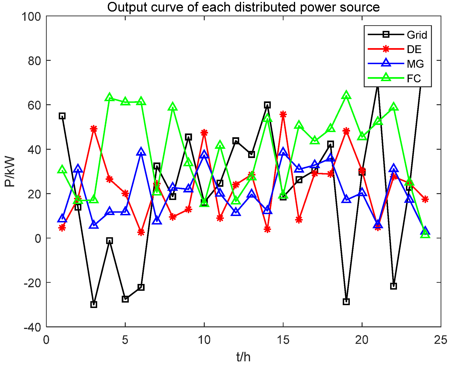
| Time (h) | Grid (KW) | DE (KW) | MT (KW) | FC (KW) | PV-WT (KW) |
|---|---|---|---|---|---|
| 1 | 54.9847 | 4.6157 | 30.5293 | 8.4419 | 2.4774 |
| 2 | 13.9208 | 17.7461 | 16.7995 | 30.9069 | 0.5377 |
| 3 | −30.0000 | 49.2007 | 17.0434 | 5.5785 | 2.6790 |
| 4 | −1.1387 | 26.5018 | 63.0595 | 11.7369 | 1.1584 |
| 5 | −27.5462 | 20.1368 | 61.1810 | 11.6811 | 1.6862 |
| 6 | −22.2145 | 2.5391 | 61.3192 | 38.5415 | 1.8147 |
| 7 | 32.4267 | 24.4806 | 20.6001 | 7.5464 | 0.0312 |
| 8 | 18.7005 | 9.4939 | 58.8034 | 22.6857 | 1.1915 |
| 9 | 45.4677 | 12.9296 | 33.7325 | 21.9738 | 1.1454 |
| 10 | 16.0335 | 47.4314 | 15.3470 | 37.2843 | 4.5908 |
| 11 | 24.6919 | 8.9679 | 41.6544 | 20.0269 | 3.4449 |
| 12 | 43.7713 | 24.0744 | 16.5186 | 11.3769 | 8.2029 |
| 13 | 37.6223 | 28.5550 | 27.3770 | 19.6472 | 8.4275 |
| 14 | 59.9395 | 3.9189 | 53.6826 | 12.2077 | 6.4023 |
| 15 | 18.4272 | 55.6835 | 19.2147 | 38.5125 | 5.9142 |
| 16 | 26.2810 | 8.2503 | 50.6074 | 30.9076 | 2.7776 |
| 17 | 30.4756 | 29.1353 | 43.6213 | 32.8522 | 3.1366 |
| 18 | 42.2725 | 28.8073 | 49.1521 | 35.8254 | 1.1007 |
| 19 | −28.6802 | 48.2836 | 64.0777 | 17.1399 | 0.8680 |
| 20 | 29.6620 | 30.3528 | 45.4651 | 20.2881 | 1.6321 |
| 21 | 69.7417 | 4.8349 | 52.3628 | 5.8072 | 2.5654 |
| 22 | −21.7034 | 27.6313 | 58.7886 | 31.1348 | 0.8406 |
| 23 | 22.8784 | 24.7073 | 25.0228 | 17.2717 | 0.3629 |
Disclaimer/Publisher’s Note: The statements, opinions and data contained in all publications are solely those of the individual author(s) and contributor(s) and not of MDPI and/or the editor(s). MDPI and/or the editor(s) disclaim responsibility for any injury to people or property resulting from any ideas, methods, instructions or products referred to in the content. |
© 2023 by the authors. Licensee MDPI, Basel, Switzerland. This article is an open access article distributed under the terms and conditions of the Creative Commons Attribution (CC BY) license (https://creativecommons.org/licenses/by/4.0/).
Share and Cite
Zhang, Y.; Lv, Y.; Zhou, Y. Research on Economic Optimal Dispatching of Microgrid Based on an Improved Bacteria Foraging Optimization. Biomimetics 2023, 8, 150. https://doi.org/10.3390/biomimetics8020150
Zhang Y, Lv Y, Zhou Y. Research on Economic Optimal Dispatching of Microgrid Based on an Improved Bacteria Foraging Optimization. Biomimetics. 2023; 8(2):150. https://doi.org/10.3390/biomimetics8020150
Chicago/Turabian StyleZhang, Yi, Yang Lv, and Yangkun Zhou. 2023. "Research on Economic Optimal Dispatching of Microgrid Based on an Improved Bacteria Foraging Optimization" Biomimetics 8, no. 2: 150. https://doi.org/10.3390/biomimetics8020150