
Subtraction-Average-Based Optimizer: A New Swarm-Inspired Metaheuristic Algorithm for Solving Optimization Problems


Abstract
:1. Introduction
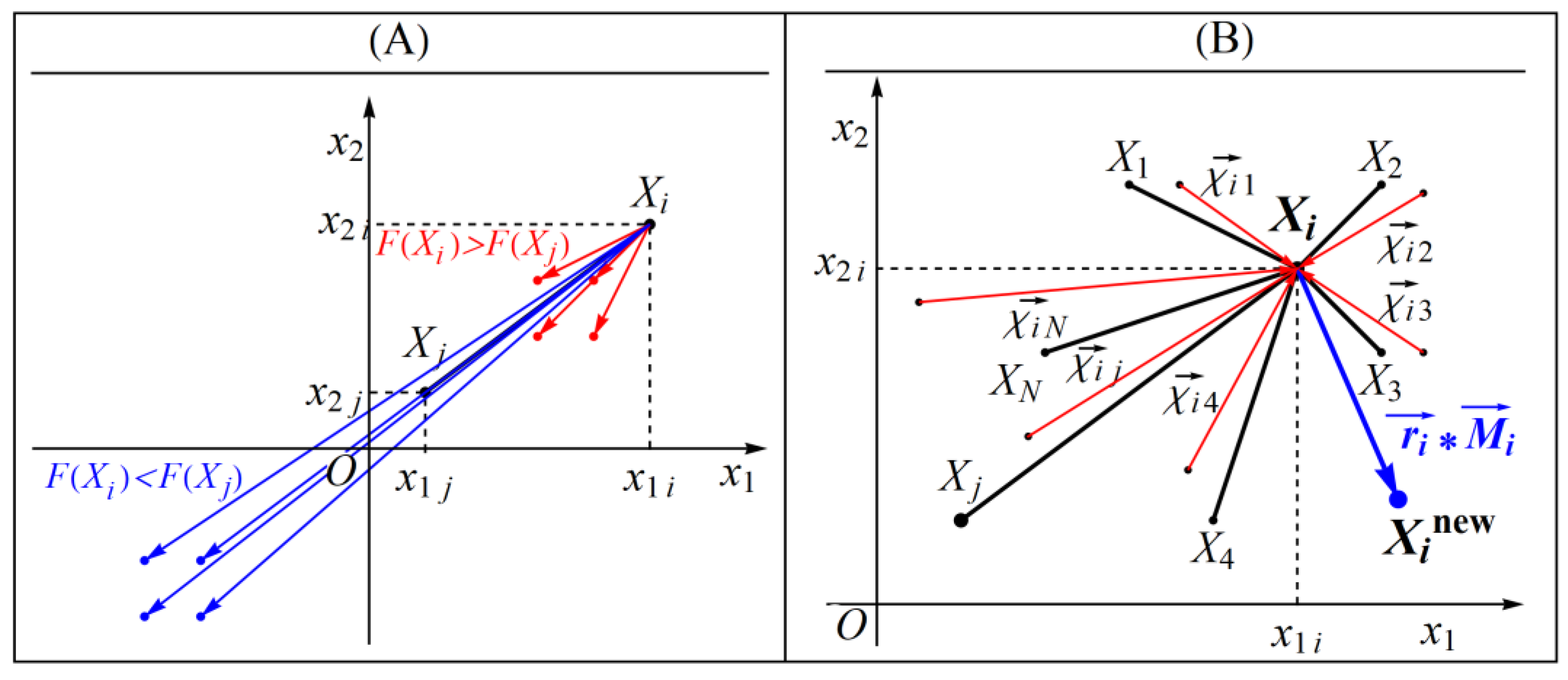
- The basic idea behind the design of the SABO is the mathematical concepts and information subtraction average of the algorithm’s search agents.
- The steps of the SABO’s implementation are described and its mathematical model is presented.
- The efficiency of the proposed SABO approach has been evaluated for fifty-two standard benchmark functions.
- The quality of the SABO’s results has been compared with the performance of twelve well-known algorithms.
- To evaluate the capability of the SABO in handling real-world applications, the proposed approach is implemented for four engineering design problems.
2. Literature Review
3. Subtraction-Average-Based Optimizer
3.1. Algorithm Initialization
3.2. Mathematical Modelling of SABO
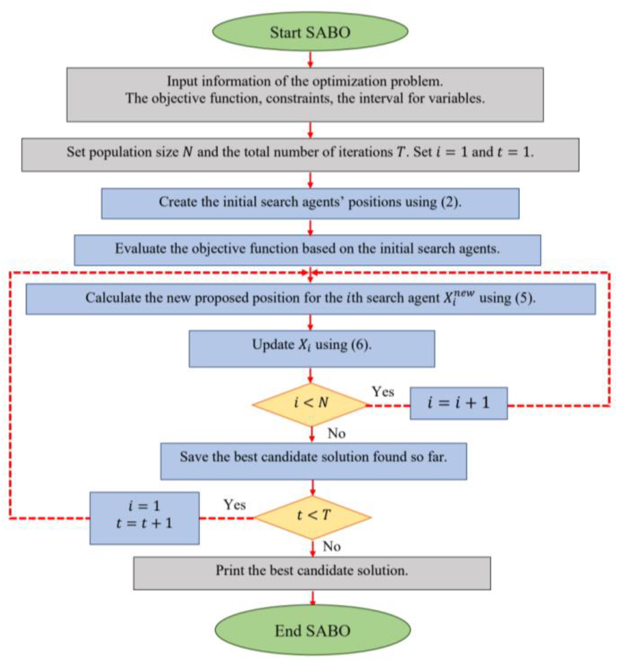
3.3. Repetition Process, Pseudocode, and Flowchart of SABO
| Algorithm 1. Pseudocode of SABO. |
| Start SABO. |
| 1. Input problem information: variables, objective function, and constraints. |
| 2. Set SABO population size (N) and iterations (T). |
| 3. Generate the initial search agents’ matrix at random using Equation (2). |
| 4. Evaluate the objective function. |
| 5. For t = 1 to T |
| 6. For i = 1 to |
| 7. Calculate new proposed position for ith SABO search agent using Equation (5). |
| 8. Update ith GAO member using Equation (6). |
| 9. end |
| 10. Save the best candidate solution so far. |
| 11. end |
| 12. Output best quasi-optimal solution obtained with the SABO. |
| End SABO. |
3.4. Computational Complexity of SABO
4. Simulation Studies and Results
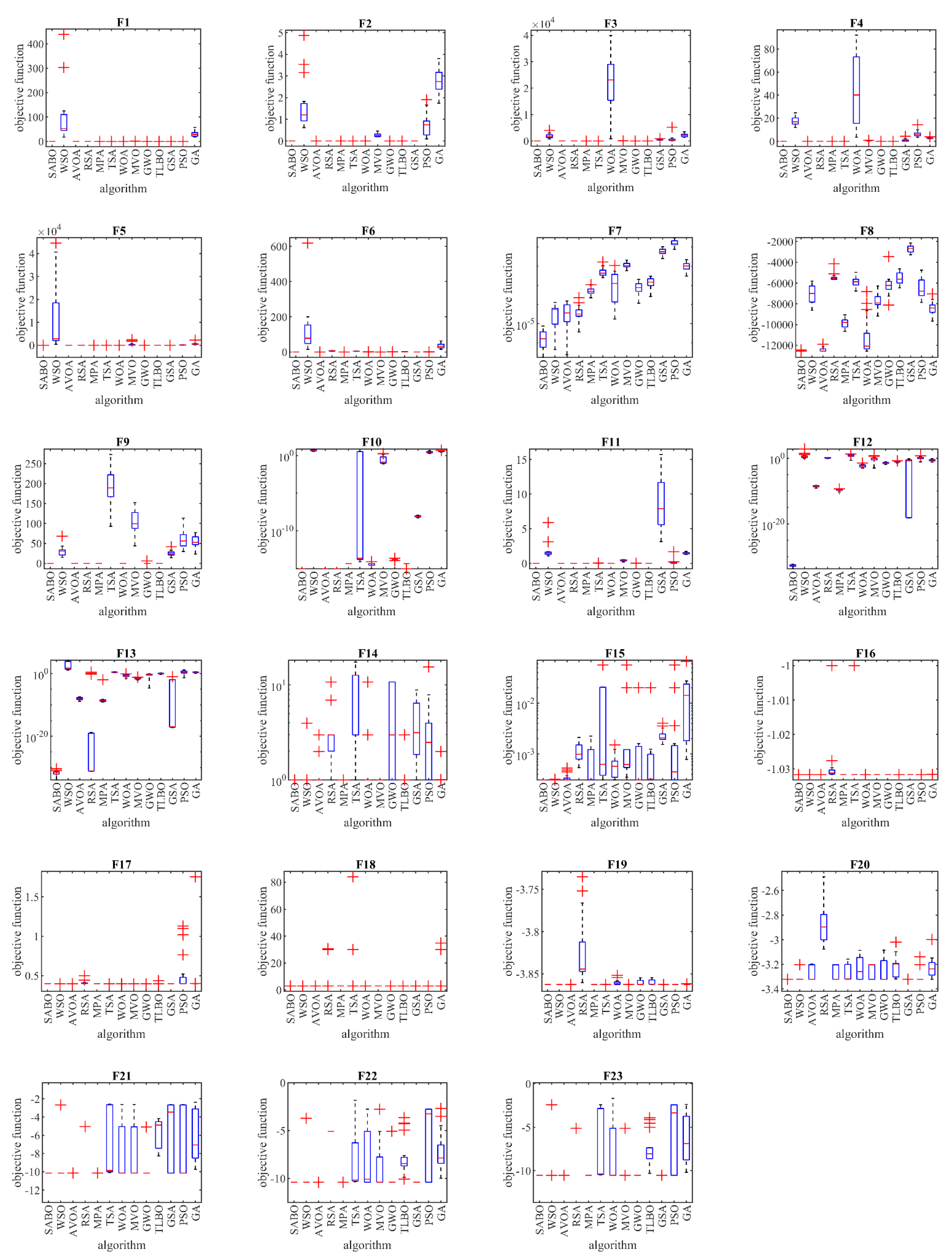
4.1. Evaluation Unimodal Functions
4.2. Evaluation High-Dimensional Multimodal Functions
4.3. Evaluation Fixed-Dimensional Multimodal Functions
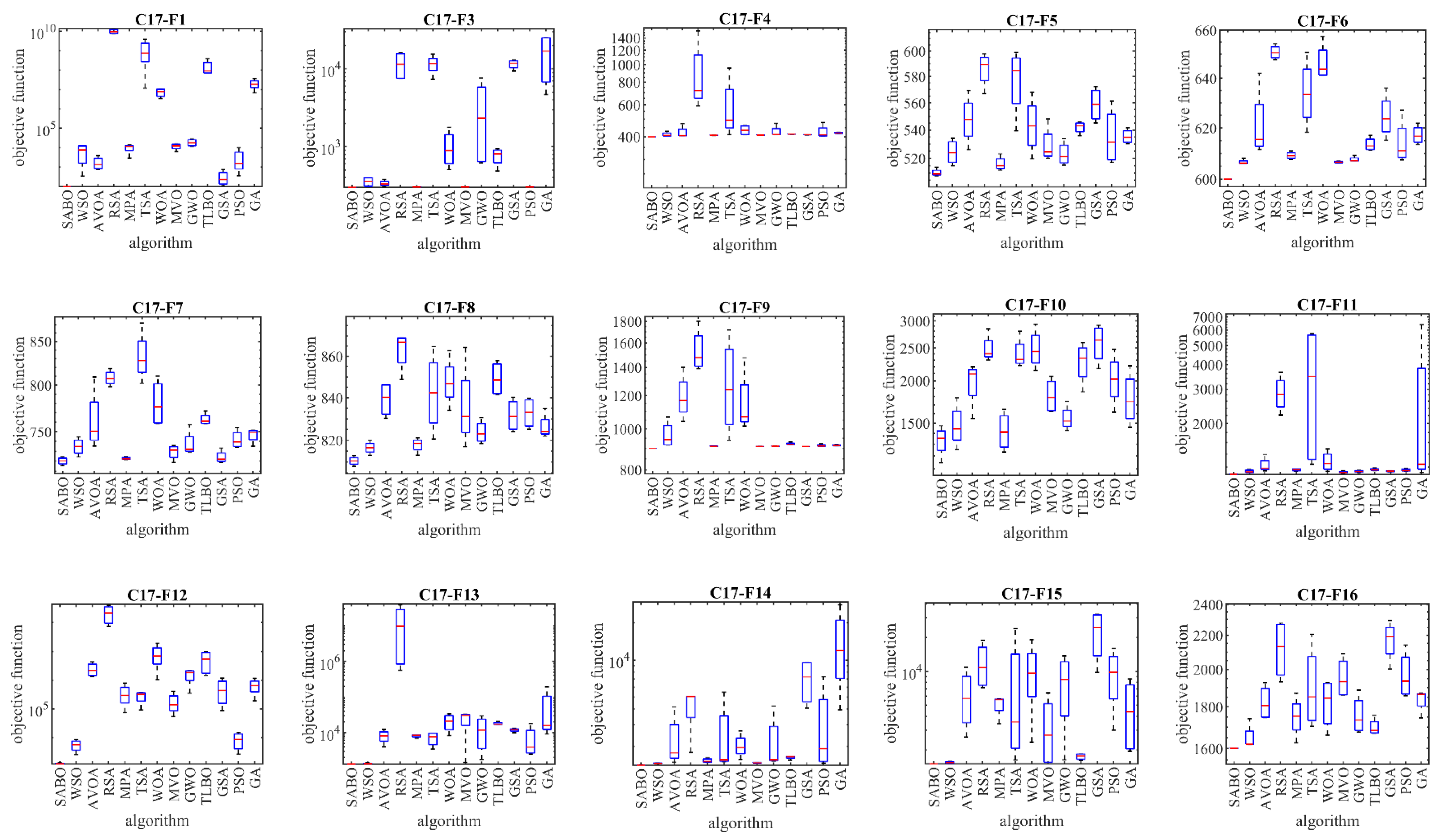
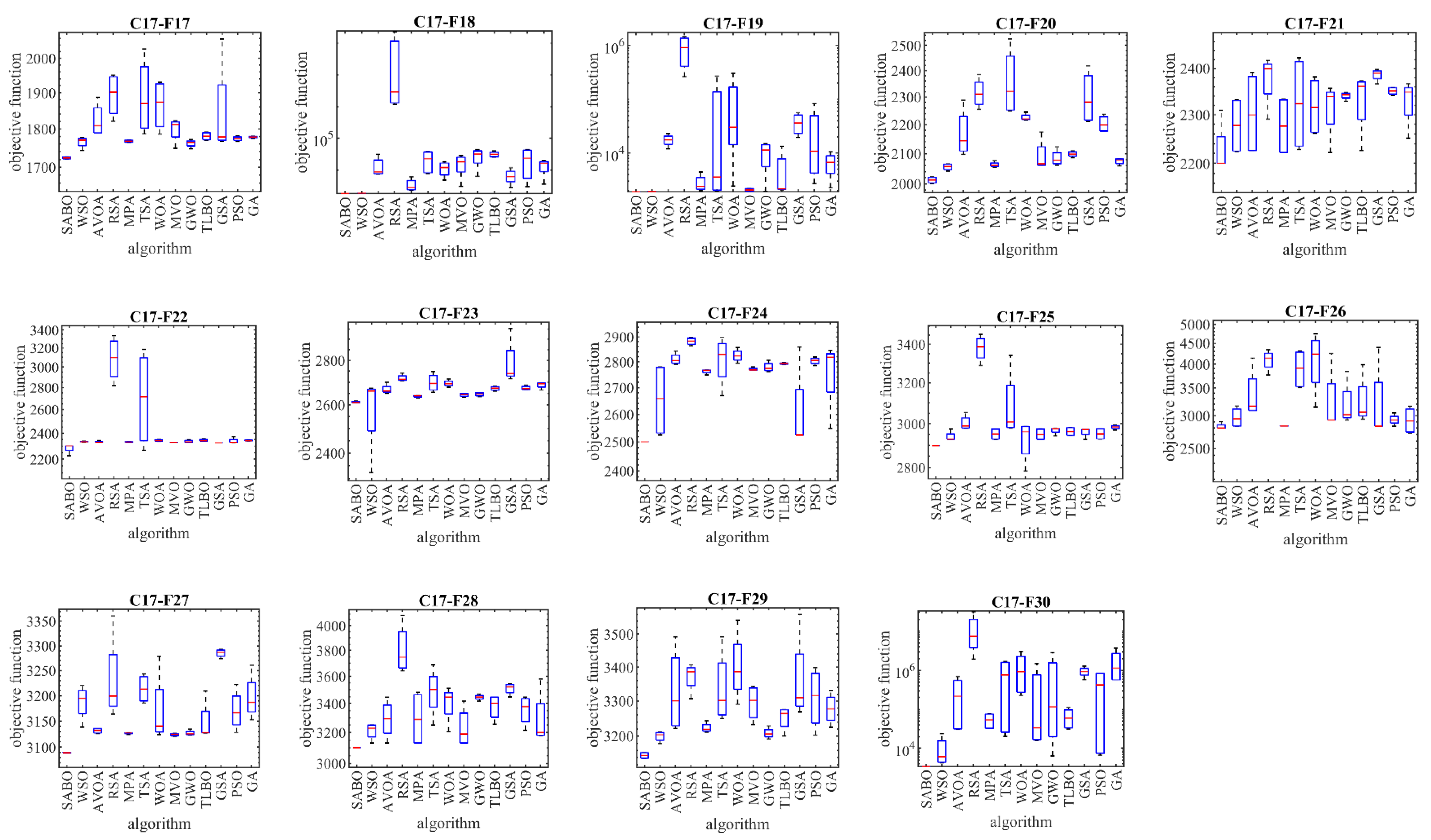
4.4. Evaluation CEC 2017 Test Suite
4.5. Statistical Analysis
4.6. Advantages and Disadvantages of SABO
5. SABO for Real-World Applications
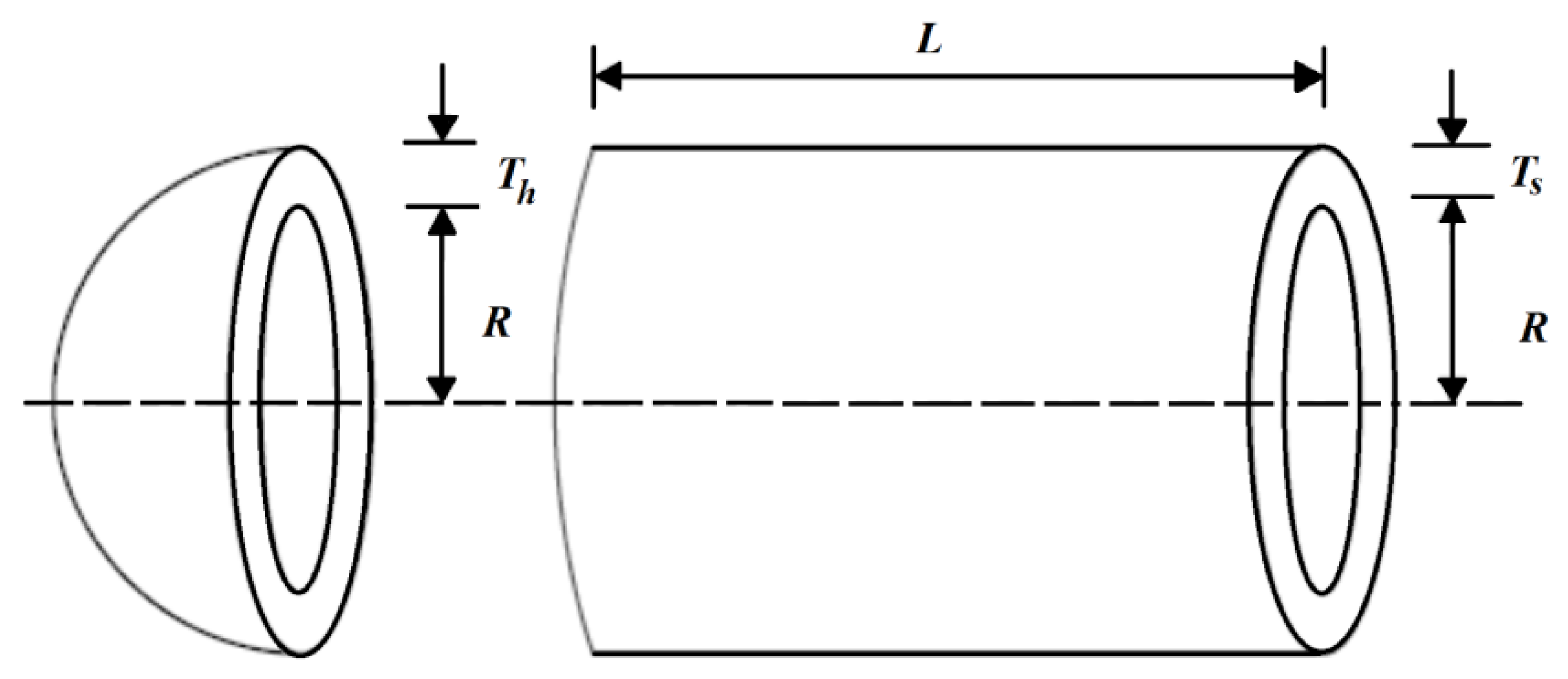
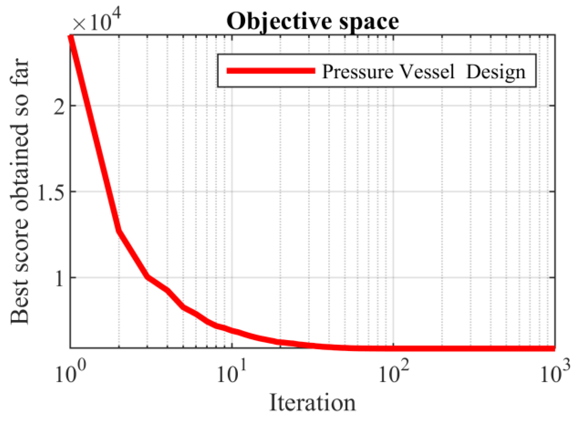
5.1. Pressure Vessel Design Problem
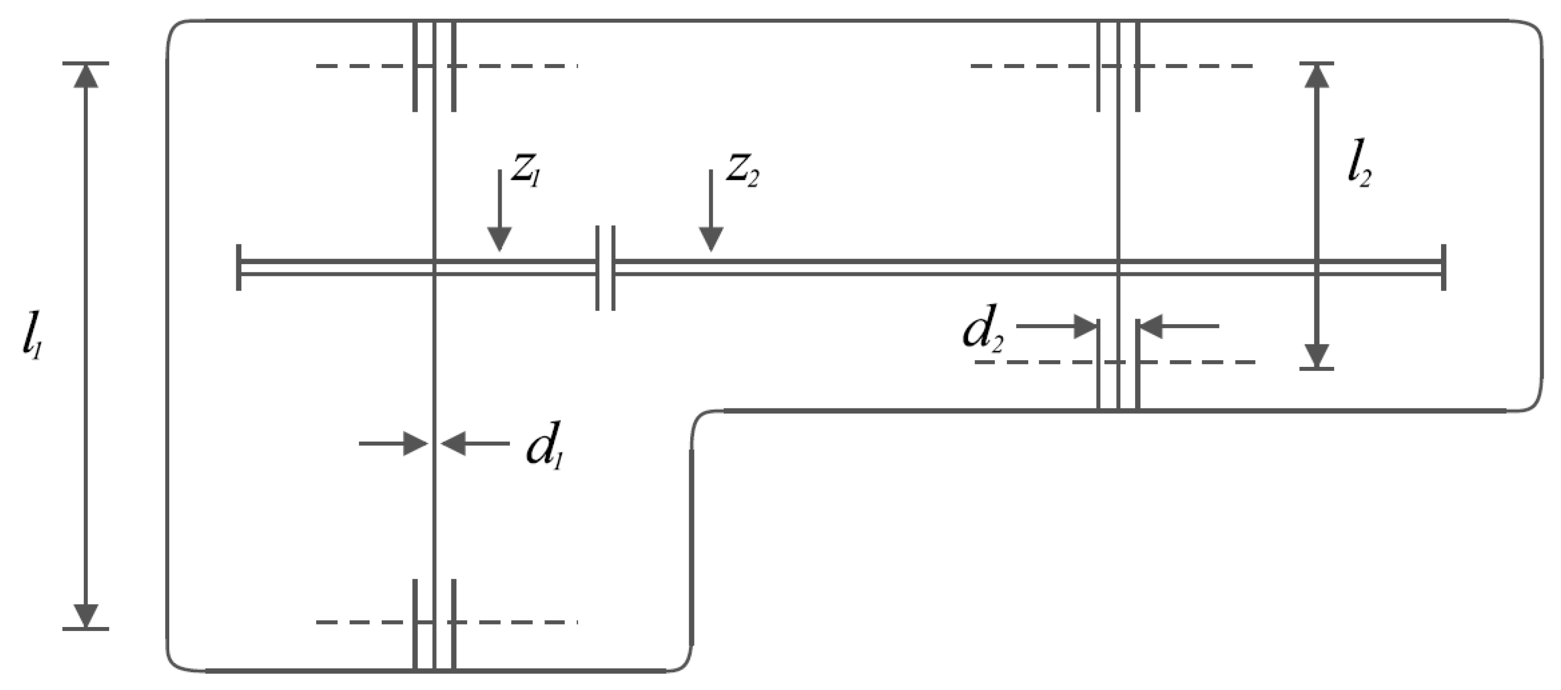
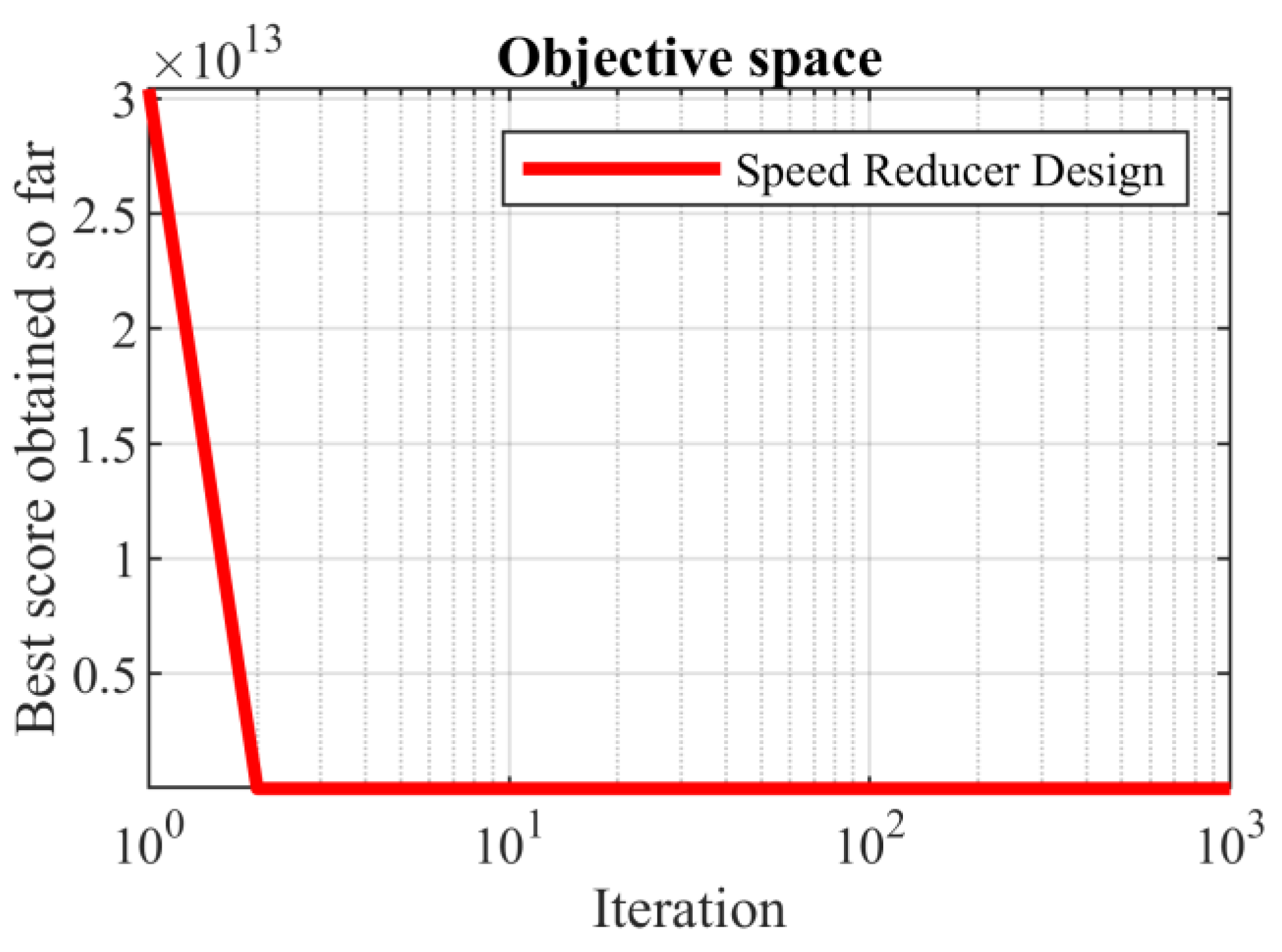
5.2. Speed Reducer Design Problem
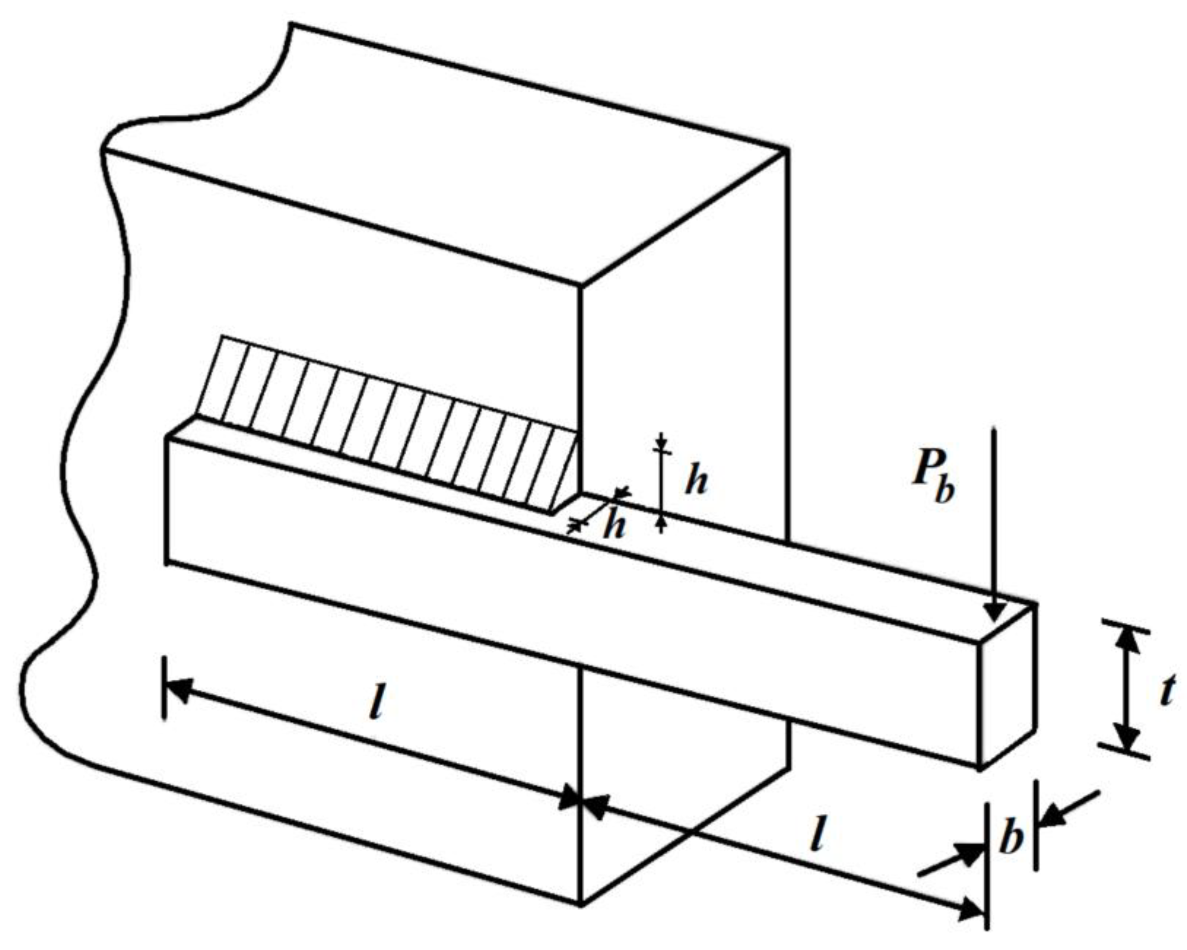
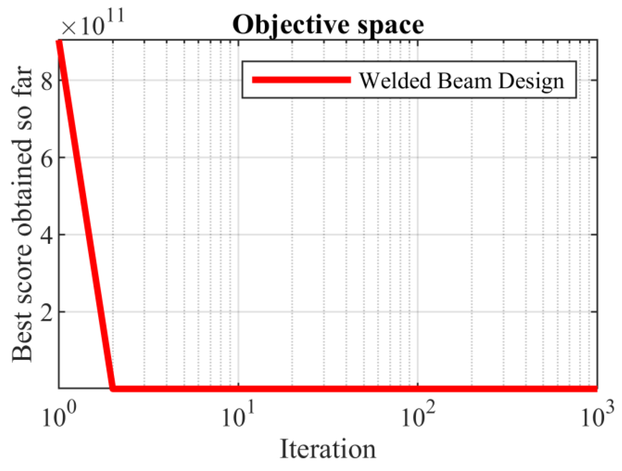
5.3. Welded Beam Design
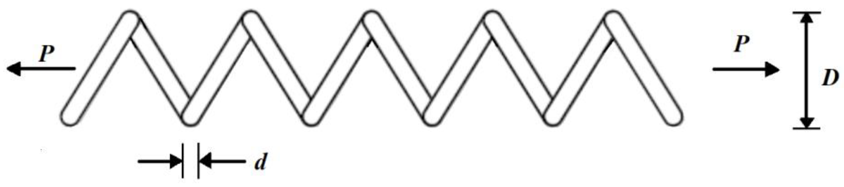
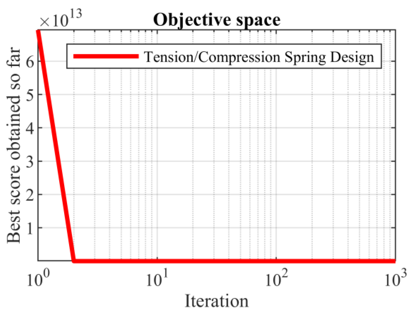
5.4. Tension/Compression Spring Design
6. Conclusions and Future Works
Author Contributions
Funding
Institutional Review Board Statement
Data Availability Statement
Acknowledgments
Conflicts of Interest
References
- Sergeyev, Y.D.; Kvasov, D.; Mukhametzhanov, M. On the efficiency of nature-inspired metaheuristics in expensive global optimization with limited budget. Sci. Rep. 2018, 8, 1–9. [Google Scholar] [CrossRef] [Green Version]
- Liberti, L.; Kucherenko, S. Comparison of deterministic and stochastic approaches to global optimization. Int. Trans. Oper. Res. 2005, 12, 263–285. [Google Scholar] [CrossRef]
- Koc, I.; Atay, Y.; Babaoglu, I. Discrete tree seed algorithm for urban land readjustment. Eng. Appl. Artif. Intell. 2022, 112, 104783. [Google Scholar] [CrossRef]
- Dehghani, M.; Trojovská, E.; Trojovský, P. A new human-based metaheuristic algorithm for solving optimization problems on the base of simulation of driving training process. Sci. Rep. 2022, 12, 9924. [Google Scholar] [CrossRef]
- Zeidabadi, F.-A.; Dehghani, M.; Trojovský, P.; Hubálovský, Š.; Leiva, V.; Dhiman, G. Archery Algorithm: A Novel Stochastic Optimization Algorithm for Solving Optimization Problems. Comput. Mater. Contin. 2022, 72, 399–416. [Google Scholar] [CrossRef]
- Yuen, M.-C.; Ng, S.-C.; Leung, M.-F.; Che, H. A metaheuristic-based framework for index tracking with practical constraints. Complex Intell. Syst. 2022, 8, 4571–4586. [Google Scholar] [CrossRef]
- Dehghani, M.; Montazeri, Z.; Malik, O.P. Energy commitment: A planning of energy carrier based on energy consumption. Electr. Eng. Electromechanics 2019, 2019, 69–72. [Google Scholar] [CrossRef]
- Dehghani, M.; Mardaneh, M.; Malik, O.P.; Guerrero, J.M.; Sotelo, C.; Sotelo, D.; Nazari-Heris, M.; Al-Haddad, K.; Ramirez-Mendoza, R.A. Genetic Algorithm for Energy Commitment in a Power System Supplied by Multiple Energy Carriers. Sustainability 2020, 12, 10053. [Google Scholar] [CrossRef]
- Dehghani, M.; Mardaneh, M.; Malik, O.P.; Guerrero, J.M.; Morales-Menendez, R.; Ramirez-Mendoza, R.A.; Matas, J.; Abusorrah, A. Energy Commitment for a Power System Supplied by Multiple Energy Carriers System using Following Optimization Algorithm. Appl. Sci. 2020, 10, 5862. [Google Scholar] [CrossRef]
- Rezk, H.; Fathy, A.; Aly, M.; Ibrahim, M.N.F. Energy management control strategy for renewable energy system based on spotted hyena optimizer. Comput. Mater. Contin. 2021, 67, 2271–2281. [Google Scholar] [CrossRef]
- Ehsanifar, A.; Dehghani, M.; Allahbakhshi, M. Calculating the leakage inductance for transformer inter-turn fault detection using finite element method. In Proceedings of the 2017 Iranian Conference on Electrical Engineering (ICEE), Tehran, Iran, 2–4 May 2017; pp. 1372–1377. [Google Scholar]
- Dehghani, M.; Montazeri, Z.; Ehsanifar, A.; Seifi, A.R.; Ebadi, M.J.; Grechko, O.M. Planning of energy carriers based on final energy consumption using dynamic programming and particle swarm optimization. Electr. Eng. Electromechanics 2018, 2018, 62–71. [Google Scholar] [CrossRef] [Green Version]
- Montazeri, Z.; Niknam, T. Energy carriers management based on energy consumption. In Proceedings of the 2017 IEEE 4th International Conference on Knowledge-Based Engineering and Innovation (KBEI), Tehran, Iran, 22 December 2017; pp. 539–543. [Google Scholar]
- Dehghani, M.; Montazeri, Z.; Malik, O. Optimal sizing and placement of capacitor banks and distributed generation in distribution systems using spring search algorithm. Int. J. Emerg. Electr. Power Syst. 2020, 21, 20190217. [Google Scholar] [CrossRef] [Green Version]
- Dehghani, M.; Montazeri, Z.; Malik, O.P.; Al-Haddad, K.; Guerrero, J.M.; Dhiman, G. A New Methodology Called Dice Game Optimizer for Capacitor Placement in Distribution Systems. Electr. Eng. Electromechanics 2020, 2020, 61–64. [Google Scholar] [CrossRef] [Green Version]
- Dehbozorgi, S.; Ehsanifar, A.; Montazeri, Z.; Dehghani, M.; Seifi, A. Line loss reduction and voltage profile improvement in radial distribution networks using battery energy storage system. In Proceedings of the 2017 IEEE 4th International Conference on Knowledge-Based Engineering and Innovation (KBEI), Tehran, Iran, 22 December 2017; pp. 215–219. [Google Scholar]
- Montazeri, Z.; Niknam, T. Optimal utilization of electrical energy from power plants based on final energy consumption using gravitational search algorithm. Electr. Eng. Electromechanics 2018, 2018, 70–73. [Google Scholar] [CrossRef] [Green Version]
- Dehghani, M.; Mardaneh, M.; Montazeri, Z.; Ehsanifar, A.; Ebadi, M.J.; Grechko, O.M. Spring search algorithm for simultaneous placement of distributed generation and capacitors. Electr. Eng. Electromechanics 2018, 2018, 68–73. [Google Scholar] [CrossRef]
- Premkumar, M.; Sowmya, R.; Jangir, P.; Nisar, K.S.; Aldhaifallah, M. A New Metaheuristic Optimization Algorithms for Brushless Direct Current Wheel Motor Design Problem. CMC-Comput. Mater. Contin. 2021, 67, 2227–2242. [Google Scholar] [CrossRef]
- de Armas, J.; Lalla-Ruiz, E.; Tilahun, S.L.; Voß, S. Similarity in metaheuristics: A gentle step towards a comparison methodology. Nat. Comput. 2022, 21, 265–287. [Google Scholar] [CrossRef]
- Trojovská, E.; Dehghani, M.; Trojovský, P. Zebra Optimization Algorithm: A New Bio-Inspired Optimization Algorithm for Solving Optimization Algorithm. IEEE Access 2022, 10, 49445–49473. [Google Scholar] [CrossRef]
- Wolpert, D.H.; Macready, W.G. No free lunch theorems for optimization. IEEE Trans. Evol. Comput. 1997, 1, 67–82. [Google Scholar] [CrossRef] [Green Version]
- Kennedy, J.; Eberhart, R. Particle swarm optimization. In Proceedings of the ICNN’95—International Conference on Neural Networks, Perth, WA, Australia, 27 November–1 December 1995; Volume 1944, pp. 1942–1948. [Google Scholar]
- Dorigo, M.; Maniezzo, V.; Colorni, A. Ant system: Optimization by a colony of cooperating agents. IEEE Trans. Syst. Man Cybern. Part B 1996, 26, 29–41. [Google Scholar] [CrossRef] [Green Version]
- Karaboga, D.; Basturk, B. Artificial bee colony (ABC) optimization algorithm for solving constrained optimization problems. In Proceedings of the International Fuzzy Systems Association World Congress, Daegu, Republic of Korea, 20–24 August 2023; pp. 789–798. [Google Scholar]
- Abualigah, L.; Abd Elaziz, M.; Sumari, P.; Geem, Z.W.; Gandomi, A.H. Reptile Search Algorithm (RSA): A nature-inspired meta-heuristic optimizer. Expert Syst. Appl. 2022, 191, 116158. [Google Scholar] [CrossRef]
- Jiang, Y.; Wu, Q.; Zhu, S.; Zhang, L. Orca predation algorithm: A novel bio-inspired algorithm for global optimization problems. Expert Syst. Appl. 2022, 188, 116026. [Google Scholar] [CrossRef]
- Faramarzi, A.; Heidarinejad, M.; Mirjalili, S.; Gandomi, A.H. Marine Predators Algorithm: A nature-inspired metaheuristic. Expert Syst. Appl. 2020, 152, 113377. [Google Scholar] [CrossRef]
- Abdollahzadeh, B.; Gharehchopogh, F.S.; Mirjalili, S. African vultures optimization algorithm: A new nature-inspired metaheuristic algorithm for global optimization problems. Comput. Ind. Eng. 2021, 158, 107408. [Google Scholar] [CrossRef]
- Hashim, F.A.; Houssein, E.H.; Hussain, K.; Mabrouk, M.S.; Al-Atabany, W. Honey Badger Algorithm: New metaheuristic algorithm for solving optimization problems. Math. Comput. Simul. 2022, 192, 84–110. [Google Scholar] [CrossRef]
- Braik, M.; Hammouri, A.; Atwan, J.; Al-Betar, M.A.; Awadallah, M.A. White Shark Optimizer: A novel bio-inspired meta-heuristic algorithm for global optimization problems. Knowl. Based Syst. 2022, 243, 108457. [Google Scholar] [CrossRef]
- Mirjalili, S.; Lewis, A. The whale optimization algorithm. Adv. Eng. Softw. 2016, 95, 51–67. [Google Scholar] [CrossRef]
- Kaur, S.; Awasthi, L.K.; Sangal, A.L.; Dhiman, G. Tunicate Swarm Algorithm: A new bio-inspired based metaheuristic paradigm for global optimization. Eng. Appl. Artif. Intell. 2020, 90, 103541. [Google Scholar] [CrossRef]
- Mirjalili, S.; Mirjalili, S.M.; Lewis, A. Grey Wolf Optimizer. Adv. Eng. Softw. 2014, 69, 46–61. [Google Scholar] [CrossRef] [Green Version]
- Chopra, N.; Ansari, M.M. Golden Jackal Optimization: A Novel Nature-Inspired Optimizer for Engineering Applications. Expert Syst. Appl. 2022, 198, 116924. [Google Scholar] [CrossRef]
- Storn, R.; Price, K. Differential evolution–a simple and efficient heuristic for global optimization over continuous spaces. J. Glob. Optim. 1997, 11, 341–359. [Google Scholar] [CrossRef]
- Goldberg, D.E.; Holland, J.H. Genetic Algorithms and Machine Learning. Mach. Learn. 1988, 3, 95–99. [Google Scholar] [CrossRef]
- Kirkpatrick, S.; Gelatt, C.D.; Vecchi, M.P. Optimization by simulated annealing. Science 1983, 220, 671–680. [Google Scholar] [CrossRef] [PubMed]
- Rashedi, E.; Nezamabadi-Pour, H.; Saryazdi, S. GSA: A gravitational search algorithm. Inf. Sci. 2009, 179, 2232–2248. [Google Scholar] [CrossRef]
- Dehghani, M.; Samet, H. Momentum search algorithm: A new meta-heuristic optimization algorithm inspired by momentum conservation law. SN Appl. Sci. 2020, 2, 1–15. [Google Scholar] [CrossRef]
- Eskandar, H.; Sadollah, A.; Bahreininejad, A.; Hamdi, M. Water cycle algorithm–A novel metaheuristic optimization method for solving constrained engineering optimization problems. Comput. Struct. 2012, 110, 151–166. [Google Scholar] [CrossRef]
- Hatamlou, A. Black hole: A new heuristic optimization approach for data clustering. Inf. Sci. 2013, 222, 175–184. [Google Scholar] [CrossRef]
- Mirjalili, S.; Mirjalili, S.M.; Hatamlou, A. Multi-verse optimizer: A nature-inspired algorithm for global optimization. Neural Comput. Appl. 2016, 27, 495–513. [Google Scholar] [CrossRef]
- Faramarzi, A.; Heidarinejad, M.; Stephens, B.; Mirjalili, S. Equilibrium optimizer: A novel optimization algorithm. Knowl. Based Syst. 2020, 191, 105190. [Google Scholar] [CrossRef]
- Kaveh, A.; Dadras, A. A novel meta-heuristic optimization algorithm: Thermal exchange optimization. Adv. Eng. Softw. 2017, 110, 69–84. [Google Scholar] [CrossRef]
- Hashim, F.A.; Hussain, K.; Houssein, E.H.; Mabrouk, M.S.; Al-Atabany, W. Archimedes optimization algorithm: A new metaheuristic algorithm for solving optimization problems. Appl. Intell. 2021, 51, 1531–1551. [Google Scholar] [CrossRef]
- Pereira, J.L.J.; Francisco, M.B.; Diniz, C.A.; Oliver, G.A.; Cunha Jr, S.S.; Gomes, G.F. Lichtenberg algorithm: A novel hybrid physics-based meta-heuristic for global optimization. Expert Syst. Appl. 2021, 170, 114522. [Google Scholar] [CrossRef]
- Hashim, F.A.; Houssein, E.H.; Mabrouk, M.S.; Al-Atabany, W.; Mirjalili, S. Henry gas solubility optimization: A novel physics-based algorithm. Future Gener. Comput. Syst. 2019, 101, 646–667. [Google Scholar] [CrossRef]
- Cuevas, E.; Oliva, D.; Zaldivar, D.; Pérez-Cisneros, M.; Sossa, H. Circle detection using electro-magnetism optimization. Inf. Sci. 2012, 182, 40–55. [Google Scholar] [CrossRef] [Green Version]
- Wei, Z.; Huang, C.; Wang, X.; Han, T.; Li, Y. Nuclear reaction optimization: A novel and powerful physics-based algorithm for global optimization. IEEE Access 2019, 7, 66084–66109. [Google Scholar] [CrossRef]
- Rao, R.V.; Savsani, V.J.; Vakharia, D. Teaching–learning-based optimization: A novel method for constrained mechanical design optimization problems. Comput. Aided Des. 2011, 43, 303–315. [Google Scholar] [CrossRef]
- Dehghani, M.; Trojovský, P. Teamwork Optimization Algorithm: A New Optimization Approach for Function Minimization/Maximization. Sensors 2021, 21, 4567. [Google Scholar] [CrossRef]
- Mohamed, A.W.; Hadi, A.A.; Mohamed, A.K. Gaining-sharing knowledge based algorithm for solving optimization problems: A novel nature-inspired algorithm. Int. J. Mach. Learn. Cybern. 2020, 11, 1501–1529. [Google Scholar] [CrossRef]
- Braik, M.; Ryalat, M.H.; Al-Zoubi, H. A novel meta-heuristic algorithm for solving numerical optimization problems: Ali Baba and the forty thieves. Neural Comput. Appl. 2022, 34, 409–455. [Google Scholar] [CrossRef]
- Al-Betar, M.A.; Alyasseri, Z.A.A.; Awadallah, M.A.; Abu Doush, I. Coronavirus herd immunity optimizer (CHIO). Neural Comput. Appl. 2021, 33, 5011–5042. [Google Scholar] [CrossRef]
- Ayyarao, T.L.; RamaKrishna, N.; Elavarasam, R.M.; Polumahanthi, N.; Rambabu, M.; Saini, G.; Khan, B.; Alatas, B. War Strategy Optimization Algorithm: A New Effective Metaheuristic Algorithm for Global Optimization. IEEE Access 2022, 10, 25073–25105. [Google Scholar] [CrossRef]
- Moghdani, R.; Salimifard, K. Volleyball premier league algorithm. Appl. Soft Comput. 2018, 64, 161–185. [Google Scholar] [CrossRef]
- Dehghani, M.; Mardaneh, M.; Guerrero, J.M.; Malik, O.; Kumar, V. Football game based optimization: An application to solve energy commitment problem. Int. J. Intell. Eng. Syst. 2020, 13, 514–523. [Google Scholar] [CrossRef]
- Awad, N.; Ali, M.; Liang, J.; Qu, B.; Suganthan, P.; Definitions, P. Evaluation Criteria for the CEC 2017 Special Session and Competition on Single Objective Real-Parameter Numerical Optimization; Technology Report; Nanyang Technological University: Singapore, 2016. [Google Scholar]
- Wilcoxon, F. Individual comparisons by ranking methods. In Breakthroughs in Statistics; Springer: Berlin/Heidelberg, Germany, 1992; pp. 196–202. [Google Scholar]
- Kannan, B.; Kramer, S.N. An augmented Lagrange multiplier based method for mixed integer discrete continuous optimization and its applications to mechanical design. J. Mech. Des. 1994, 116, 405–411. [Google Scholar] [CrossRef]
- Gandomi, A.H.; Yang, X.-S. Benchmark problems in structural optimization. In Computational Optimization, Methods and Algorithms; Springer: Berlin/Heidelberg, Germany, 2011; pp. 259–281. [Google Scholar]
- Mezura-Montes, E.; Coello, C.A.C. Useful infeasible solutions in engineering optimization with evolutionary algorithms. In Proceedings of the Mexican International Conference on Artificial Intelligence, Monterrey, Mexico, 14–18 November 2005; pp. 652–662. [Google Scholar]


| Algorithm | Parameter | Value |
|---|---|---|
| GA | ||
| Type | Real coded | |
| Selection | Roulette wheel (Proportionate) | |
| Crossover | Whole arithmetic (Probability = 0.8, ) | |
| Mutation | Gaussian (Probability = 0.05) | |
| PSO | ||
| Topology | Fully connected | |
| Cognitive and social constant | (C1, C2) = | |
| Inertia weight | Linear reduction from 0.9 to 0.1 | |
| Velocity limit | 10% of dimension range | |
| GSA | ||
| Alpha, G0, Rnorm, Rpower | 20, 100, 2, 1 | |
| TLBO | ||
| TF: teaching factor | TF = round | |
| random number | rand is a random number between | |
| GWO | ||
| Convergence parameter (a) | a: Linear reduction from 2 to 0. | |
| MVO | ||
| Wormhole existence probability (WEP) | Min(WEP) = 0.2 and Max(WEP) = 1. | |
| Exploitation accuracy over the iterations (p) | p = 6. | |
| WOA | ||
| Convergence parameter (a) | a: Linear reduction from 2 to 0. | |
| r is a random vector in [0–1] | ||
| l is a random number in | ||
| TSA | ||
| Pmin and Pmax | 1, 4 | |
| c1, c2, c3 | Random numbers lie in the range of | |
| MPA | ||
| Constant number | p = 0.5 | |
| Random vector | R is a vector of uniform random numbers in | |
| Fish Aggregating Devices (FADs) | FADs = 0.2 | |
| Binary vector | U = 0 or 1 | |
| RSA | ||
| Sensitive parameter | ||
| Sensitive parameter | ||
| Evolutionary Sense (ES) | ES: randomly decreasing values between 2 and −2 | |
| AVOA | ||
| L1, L2 | 0.8, 0.2 | |
| w | 2.5 | |
| P1, P2, P3 | 0.6, 0.4, 0.6 | |
| WSO | ||
| Fmin and Fmax | 0.07, 0.75 | |
| τ, ao, a1, a2 | 4.125, 6.25, 100, 0.0005 |
| SABO | WSO | AVOA | RSA | MPA | TSA | WOA | MVO | GWO | TLBO | GSA | PSO | GA | ||
|---|---|---|---|---|---|---|---|---|---|---|---|---|---|---|
| F1 | Mean | 0 | 94.68556 | 0 | 0 | 6.88 × 10−50 | 6.07 × 10−47 | 2.4 × 10−155 | 0.144595 | 3.87 × 10−58 | 8.14 × 10−75 | 9.33 × 10⁻¹⁷ | 0.022702 | 30.50201 |
| Best | 0 | 17.42507 | 0 | 0 | 2.13 × 10−51 | 1.01 × 10−50 | 1.4 × 10−167 | 0.071226 | 7.24 × 10−61 | 5.32 × 10−77 | 4.88 × 10⁻¹⁷ | 4.43 × 10⁻⁶ | 17.92696 | |
| Worst | 0 | 439.1736 | 0 | 0 | 5.24 × 10−49 | 6.22 × 10−46 | 2.1 × 10−154 | 0.269577 | 6.86 × 10−57 | 1.07 × 10−73 | 1.92 × 10⁻¹⁶ | 0.158149 | 56.92799 | |
| Std | 0 | 101.7604 | 0 | 0 | 1.26 × 10−49 | 1.64 × 10−46 | 6.1 × 10−155 | 0.05687 | 1.52 × 10−57 | 2.34 × 10−74 | 3.76 × 10⁻¹⁷ | 0.046942 | 10.46286 | |
| Median | 0 | 51.91934 | 0 | 0 | 1.97 × 10−50 | 4.04 × 10−48 | 3.7 × 10−158 | 0.122317 | 1.34 × 10−59 | 1.27 × 10−75 | 8.64 × 10⁻¹⁷ | 0.001314 | 28.19897 | |
| Rank | 1 | 11 | 1 | 1 | 5 | 6 | 2 | 9 | 4 | 3 | 7 | 8 | 10 | |
| F2 | Mean | 0 | 1.575136 | 1.2 × 10−266 | 0 | 3 × 10⁻²⁸ | 1.11 × 10⁻²⁸ | 5.7 × 10−103 | 0.26717 | 7.97 × 10⁻³⁵ | 6.09 × 10−39 | 5.22 × 10⁻⁸ | 0.731055 | 2.788395 |
| Best | 0 | 0.609154 | 2.3 × 10−301 | 0 | 3.21 × 10⁻³¹ | 1.02 × 10⁻³⁰ | 3.8 × 10−114 | 0.189084 | 1.45 × 10⁻³⁵ | 3.25 × 10−40 | 3.41 × 10⁻⁸ | 0.089719 | 1.745356 | |
| Worst | 0 | 4.873582 | 2.5 × 10−265 | 0 | 1.5 × 10⁻²⁷ | 5.72 × 10⁻²⁸ | 5.3 × 10−102 | 0.457641 | 2.54 × 10⁻³⁴ | 3.59 × 10−38 | 7.3 × 10⁻⁸ | 1.908597 | 3.806556 | |
| Std | 0 | 1.088388 | 0 | 0 | 4.14 × 10⁻²⁸ | 1.6 × 10⁻²⁸ | 1.5 × 10−102 | 0.075891 | 6.78 × 10⁻³⁵ | 9.92 × 10−39 | 1.14 × 10⁻⁸ | 0.534508 | 0.544788 | |
| Median | 0 | 1.202514 | 7.1 × 10−287 | 0 | 1.17 × 10⁻²⁸ | 3.98 × 10⁻²⁹ | 9 × 10−108 | 0.253065 | 6.46 × 10⁻³⁵ | 2.45 × 10−39 | 5.16 × 10⁻⁸ | 0.743555 | 2.741555 | |
| Rank | 1 | 11 | 2 | 1 | 7 | 6 | 3 | 9 | 5 | 4 | 8 | 10 | 12 | |
| F3 | Mean | 0 | 1806.78 | 0 | 0 | 5.38 × 10⁻¹² | 1.31 × 10⁻¹² | 21,771.78 | 14.05216 | 4.07 × 10⁻¹⁵ | 1.87 × 10⁻²⁵ | 434.0065 | 643.4302 | 2168.983 |
| Best | 0 | 687.9998 | 0 | 0 | 2.9 × 10⁻²⁵ | 1.4 × 10⁻¹⁷ | 804.8555 | 5.810656 | 3.22 × 10⁻¹⁹ | 1.87 × 10⁻²⁹ | 235.952 | 36.45082 | 1424.187 | |
| Worst | 0 | 4051.23 | 0 | 0 | 7.54 × 10⁻¹¹ | 1.89 × 10⁻¹¹ | 39,997.34 | 29.19354 | 4.98 × 10⁻¹⁴ | 1.97 × 10⁻²⁴ | 905.2518 | 5210.771 | 3458.935 | |
| Std | 0 | 827.0454 | 0 | 0 | 1.71 × 10⁻¹¹ | 4.22 × 10⁻¹² | 10,690.48 | 6.15891 | 1.13 × 10⁻¹⁴ | 4.64 × 10⁻²⁵ | 157.388 | 1118.449 | 639.6914 | |
| Median | 0 | 1619.412 | 0 | 0 | 2.19 × 10⁻¹³ | 2.52 × 10⁻¹⁴ | 23,134.65 | 12.09381 | 2.84 × 10⁻¹⁶ | 1.35 × 10⁻²⁶ | 418.4298 | 284.912 | 2100.7 | |
| Rank | 1 | 9 | 1 | 1 | 5 | 4 | 11 | 6 | 3 | 2 | 7 | 8 | 10 | |
| F4 | Mean | 0 | 17.76181 | 2 × 10−263 | 0 | 4.29 × 10⁻¹⁹ | 0.004673 | 44.49878 | 0.52347 | 1.32 × 10⁻¹⁴ | 3.14 × 10⁻³⁰ | 0.763785 | 6.431779 | 2.829395 |
| Best | 0 | 11.90369 | 0 | 0 | 9.98 × 10⁻²⁰ | 3.08 × 10⁻⁵ | 3.549529 | 0.290684 | 3.65 × 10⁻¹⁶ | 1.45 × 10⁻³¹ | 1.23 × 10⁻⁸ | 3.435068 | 2.216469 | |
| Worst | 0 | 24.61971 | 3.6 × 10−262 | 0 | 1.39 × 10⁻¹⁸ | 0.026002 | 92.11975 | 0.898058 | 5.88 × 10⁻¹⁴ | 1.33 × 10⁻²⁹ | 4.299889 | 14.35043 | 3.992738 | |
| Std | 0 | 3.607365 | 0 | 0 | 3.25 × 10⁻¹⁹ | 0.006495 | 30.23659 | 0.163563 | 1.68 × 10⁻¹⁴ | 3.51 × 10⁻³⁰ | 1.049333 | 2.439277 | 0.466936 | |
| Median | 0 | 16.86055 | 2.9 × 10−282 | 0 | 3.93 × 10⁻¹⁹ | 0.003083 | 40.15902 | 0.5337 | 7.33 × 10⁻¹⁵ | 1.86 × 10⁻³⁰ | 0.402748 | 6.046926 | 2.783478 | |
| Rank | 1 | 11 | 2 | 1 | 4 | 6 | 12 | 7 | 5 | 3 | 8 | 10 | 9 | |
| F5 | Mean | 0.197101 | 11,081.32 | 1.87205 | 11.53391 | 23.55614 | 28.42991 | 27.20948 | 392.7405 | 26.99155 | 26.88666 | 26.39314 | 84.19977 | 595.3854 |
| Best | 0.003263 | 455.9772 | 1.58657 | 8.2 × 10⁻²⁹ | 22.95066 | 26.0171 | 26.53351 | 24.75643 | 26.01628 | 25.61541 | 25.88273 | 11.41045 | 228.808 | |
| Worst | 0.81947 | 44,603 | 2.13145 | 28.99015 | 24.83591 | 29.21115 | 28.51838 | 2433.592 | 27.94714 | 28.74413 | 27.72119 | 178.5254 | 2257.058 | |
| Std | 0.215288 | 14,373.09 | 1.542075 | 14.49384 | 0.436322 | 0.779248 | 0.474719 | 735.2203 | 0.5881 | 0.964054 | 0.426365 | 44.9786 | 424.9867 | |
| Median | 0.111639 | 2840.274 | 1.47245 | 1.08 × 10⁻²⁸ | 23.42466 | 28.82636 | 27.0195 | 30.39723 | 27.11413 | 26.45399 | 26.28991 | 87.48235 | 475.573 | |
| Rank | 1 | 13 | 2 | 3 | 4 | 9 | 8 | 11 | 7 | 6 | 5 | 10 | 12 | |
| F6 | Mean | 0 | 119.0172 | 6.52 × 10⁻⁸ | 6.319044 | 1.77 × 10⁻⁹ | 3.683762 | 0.086202 | 0.153294 | 0.636332 | 1.116967 | 1.07 × 10⁻¹⁶ | 0.082637 | 34.14746 |
| Best | 0 | 15.05144 | 4.73 × 10⁻⁹ | 3.88797 | 6.98 × 10⁻¹⁰ | 2.821592 | 0.002679 | 0.092788 | 0.249403 | 0.487407 | 4.96 × 10⁻¹⁷ | 5.23 × 10⁻⁵ | 15.61244 | |
| Worst | 0 | 618.6501 | 2.46 × 10⁻⁷ | 7.452363 | 4.45 × 10⁻⁹ | 4.79066 | 0.429712 | 0.2525 | 1.258956 | 1.907377 | 1.92 × 10⁻¹⁶ | 1.549095 | 62.76702 | |
| Std | 0 | 131.4271 | 5.56 × 10⁻⁸ | 1.201026 | 9.43 × 10⁻¹⁰ | 0.543926 | 0.110313 | 0.039617 | 0.309366 | 0.409251 | 3.8 × 10⁻¹⁷ | 0.345263 | 13.54999 | |
| Median | 0 | 78.07582 | 5.69 × 10⁻⁸ | 6.999263 | 1.41 × 10⁻⁹ | 3.565372 | 0.03592 | 0.148684 | 0.501812 | 1.043402 | 9.84 × 10⁻¹⁷ | 0.002623 | 31.68218 | |
| Rank | 1 | 13 | 4 | 11 | 3 | 10 | 6 | 7 | 8 | 9 | 2 | 5 | 12 | |
| F7 | Mean | 2.38 × 10⁻⁶ | 4.93 × 10⁻⁵ | 5.44 × 10⁻⁵ | 4.88 × 10⁻⁵ | 0.00056 | 0.005326 | 0.002244 | 0.011754 | 0.00091 | 0.001542 | 0.059762 | 0.168645 | 0.010589 |
| Best | 1.74 × 10⁻⁷ | 4.44 × 10⁻⁷ | 2.41 × 10⁻⁷ | 3.72 × 10⁻⁶ | 0.000225 | 0.002506 | 1.76 × 10⁻⁵ | 0.005824 | 0.000117 | 0.000261 | 0.024813 | 0.074626 | 0.003032 | |
| Worst | 7.52 × 10⁻⁶ | 0.000128 | 0.000152 | 0.000226 | 0.001089 | 0.016372 | 0.010815 | 0.020623 | 0.00202 | 0.003007 | 0.102681 | 0.293086 | 0.021939 | |
| Std | 1.98 × 10⁻⁶ | 3.94 × 10⁻⁵ | 5.06 × 10⁻⁵ | 5.09 × 10⁻⁵ | 0.000258 | 0.003333 | 0.002743 | 0.004162 | 0.000569 | 0.000772 | 0.021243 | 0.060668 | 0.004819 | |
| Median | 1.63 × 10⁻⁶ | 5.39 × 10⁻⁵ | 3.64 × 10⁻⁵ | 3.21 × 10⁻⁵ | 0.00048 | 0.004299 | 0.001254 | 0.010535 | 0.000758 | 0.001479 | 0.056525 | 0.152506 | 0.010178 | |
| Rank | 1 | 3 | 4 | 2 | 5 | 9 | 8 | 11 | 6 | 7 | 12 | 13 | 10 | |
| Sum rank | 7 | 71 | 16 | 20 | 33 | 50 | 50 | 60 | 38 | 34 | 49 | 64 | 75 | |
| Mean rank | 1 | 10.14286 | 2.285714 | 2.857143 | 4.714286 | 7.142857 | 7.142857 | 8.571429 | 5.428571 | 4.857143 | 7 | 9.142857 | 10.71429 | |
| Total rank | 1 | 11 | 2 | 3 | 4 | 8 | 8 | 9 | 6 | 5 | 7 | 10 | 12 | |
| SABO | WSO | AVOA | RSA | MPA | TSA | WOA | MVO | GWO | TLBO | GSA | PSO | GA | ||
|---|---|---|---|---|---|---|---|---|---|---|---|---|---|---|
| F8 | Mean | −12,563.1 | −7037.55 | −12,433.2 | −5458.28 | −9865.61 | −5913.41 | −11,247.2 | −7742.72 | −6220.73 | −5521.56 | −2689.18 | −6500.96 | −8421.5 |
| Best | −12,569.5 | −8624.3 | −12,569.5 | −5656.04 | −10,653.2 | −6776.47 | −12,569.2 | −9182.08 | −8101.01 | −6451.23 | −3269.84 | −7862.41 | −9681.18 | |
| Worst | −12,447.1 | −5826.04 | −11,896.8 | −4124.78 | −9067.64 | −4968.21 | −6824.1 | −6283.06 | −3450.14 | −4631.24 | −2140.43 | −4751.67 | −7028.99 | |
| Std | 27.32588 | 840.3862 | 197.7043 | 345.5191 | 478.9808 | 494.6759 | 1769.136 | 677.1584 | 896.6881 | 562.8207 | 341.7721 | 885.9265 | 641.2242 | |
| Median | −12,569.5 | −7012.04 | −12,569.5 | −5531.08 | −9792.7 | −5881.29 | −12,081.1 | −7915.87 | −6226.44 | −5625.4 | −2654.18 | −6783.5 | −8399.11 | |
| Rank | 1 | 7 | 2 | 12 | 4 | 10 | 3 | 6 | 9 | 11 | 13 | 8 | 5 | |
| F9 | Mean | 0 | 30.53863 | 0 | 0 | 0 | 190.2096 | 0 | 104.0543 | 0.297985 | 0 | 25.07295 | 60.31323 | 54.68123 |
| Best | 0 | 15.22149 | 0 | 0 | 0 | 92.78168 | 0 | 43.82732 | 0 | 0 | 13.92943 | 29.84883 | 23.23239 | |
| Worst | 0 | 68.24684 | 0 | 0 | 0 | 273.0471 | 0 | 152.2773 | 5.959691 | 0 | 41.78816 | 113.4265 | 76.90086 | |
| Std | 0 | 11.93438 | 0 | 0 | 0 | 40.82636 | 0 | 28.71635 | 1.332627 | 0 | 6.256114 | 21.62223 | 13.80758 | |
| Median | 0 | 30.62966 | 0 | 0 | 0 | 189.0894 | 0 | 99.60579 | 0 | 0 | 23.879 | 56.24334 | 52.61443 | |
| Rank | 1 | 4 | 1 | 1 | 1 | 8 | 1 | 7 | 2 | 1 | 3 | 6 | 5 | |
| F10 | Mean | 8.88 × 10⁻¹⁶ | 4.901082 | 8.88 × 10⁻¹⁶ | 8.88 × 10⁻¹⁶ | 4.44 × 10⁻¹⁵ | 1.452865 | 4.26 × 10⁻¹⁵ | 0.451449 | 1.6 × 10⁻¹⁴ | 4.26 × 10⁻¹⁵ | 8.12 × 10⁻⁹ | 2.739329 | 3.5751 |
| Best | 8.88 × 10⁻¹⁶ | 3.530049 | 8.88 × 10⁻¹⁶ | 8.88 × 10⁻¹⁶ | 4.44 × 10⁻¹⁵ | 7.99 × 10⁻¹⁵ | 8.88 × 10⁻¹⁶ | 0.078241 | 1.15 × 10⁻¹⁴ | 8.88 × 10⁻¹⁶ | 5.45 × 10⁻⁹ | 1.778035 | 2.881962 | |
| Worst | 8.88 × 10⁻¹⁶ | 6.874831 | 8.88 × 10⁻¹⁶ | 8.88 × 10⁻¹⁶ | 4.44 × 10⁻¹⁵ | 3.447315 | 7.99 × 10⁻¹⁵ | 1.799202 | 2.22 × 10⁻¹⁴ | 4.44 × 10⁻¹⁵ | 1.23 × 10⁻⁸ | 4.38263 | 4.641967 | |
| Std | 0 | 0.939579 | 0 | 0 | 0 | 1.654267 | 2.44 × 10⁻¹⁵ | 0.574717 | 2.79 × 10⁻¹⁵ | 7.94 × 10⁻¹⁶ | 1.67 × 10⁻⁹ | 0.715238 | 0.396644 | |
| Median | 8.88 × 10⁻¹⁶ | 4.668923 | 8.88 × 10⁻¹⁶ | 8.88 × 10⁻¹⁶ | 4.44 × 10⁻¹⁵ | 2.22 × 10⁻¹⁴ | 4.44 × 10⁻¹⁵ | 0.131373 | 1.51 × 10⁻¹⁴ | 4.44 × 10⁻¹⁵ | 7.81 × 10⁻⁹ | 2.604421 | 3.62958 | |
| Rank | 1 | 10 | 1 | 1 | 3 | 7 | 2 | 6 | 4 | 2 | 5 | 8 | 9 | |
| F11 | Mean | 0 | 1.70897 | 0 | 0 | 0 | 0.008334 | 0 | 0.412213 | 0.000451 | 0 | 8.687165 | 0.156717 | 1.473471 |
| Best | 0 | 1.076151 | 0 | 0 | 0 | 0 | 0 | 0.191432 | 0 | 0 | 3.135355 | 0.001467 | 1.288095 | |
| Worst | 0 | 5.872952 | 0 | 0 | 0 | 0.067031 | 0 | 0.535573 | 0.009011 | 0 | 15.71589 | 1.662839 | 1.725859 | |
| Std | 0 | 1.0671 | 0 | 0 | 0 | 0.01536 | 0 | 0.099926 | 0.002015 | 0 | 3.751821 | 0.360388 | 0.123868 | |
| Median | 0 | 1.425853 | 0 | 0 | 0 | 0 | 0 | 0.430656 | 0 | 0 | 7.888906 | 0.060533 | 1.447709 | |
| Rank | 1 | 7 | 1 | 1 | 1 | 3 | 1 | 5 | 2 | 1 | 8 | 4 | 6 | |
| F12 | Mean | 2.63 × 10⁻³³ | 34.6973 | 2.86 × 10⁻⁹ | 1.314643 | 2.08 × 10⁻¹⁰ | 6.293599 | 0.00738 | 1.251754 | 0.035525 | 0.08398 | 0.187602 | 1.583141 | 0.274894 |
| Best | 2.13 × 10⁻³⁴ | 0.938867 | 7.56 × 10⁻¹⁰ | 0.720132 | 6.03 × 10⁻¹¹ | 0.216628 | 0.000964 | 0.001016 | 0.012978 | 0.035054 | 5.91 × 10⁻¹⁹ | 0.074149 | 0.060841 | |
| Worst | 5.73 × 10⁻³³ | 597.7173 | 5.14 × 10⁻⁹ | 1.629701 | 4.75 × 10⁻¹⁰ | 17.71439 | 0.033587 | 6.169218 | 0.07355 | 0.170805 | 0.634329 | 5.095104 | 0.650842 | |
| Std | 1.57 × 10⁻³³ | 132.7047 | 1.34 × 10⁻⁹ | 0.330125 | 9.3 × 10⁻¹¹ | 4.26837 | 0.007596 | 1.62632 | 0.018405 | 0.032215 | 0.20951 | 1.251155 | 0.138648 | |
| Median | 2.62 × 10⁻³³ | 3.696076 | 2.7 × 10⁻⁹ | 1.525877 | 1.93 × 10⁻¹⁰ | 6.01544 | 0.005285 | 0.807143 | 0.029024 | 0.082474 | 0.155493 | 1.381006 | 0.264424 | |
| Rank | 1 | 13 | 3 | 10 | 2 | 12 | 4 | 9 | 5 | 6 | 7 | 11 | 8 | |
| F13 | Mean | 6.7 × 10⁻³² | 4239.934 | 1.43 × 10⁻⁸ | 0.355 | 0.000567 | 2.81567 | 0.275667 | 0.02976 | 0.495453 | 1.030391 | 0.007691 | 4.690251 | 2.707835 |
| Best | 1.14 × 10⁻³⁴ | 12.39891 | 1.5 × 10⁻⁹ | 6.53 × 10⁻³² | 8.3 × 10⁻¹⁰ | 2.029692 | 0.032988 | 0.009002 | 2.27 × 10⁻⁵ | 0.529644 | 5.94 × 10⁻¹⁸ | 0.04709 | 1.291959 | |
| Worst | 4.34 × 10⁻³¹ | 17,963.65 | 3.86 × 10⁻⁸ | 2.9 | 0.011347 | 3.832826 | 0.781805 | 0.079707 | 0.852264 | 1.626638 | 0.098883 | 14.57619 | 3.940231 | |
| Std | 1.2 × 10⁻³¹ | 7400.496 | 1.17 × 10⁻⁸ | 0.849443 | 0.002537 | 0.479843 | 0.209069 | 0.018477 | 0.219041 | 0.29138 | 0.022003 | 4.549049 | 0.754476 | |
| Median | 3.38 × 10⁻³² | 55.13453 | 1.1 × 10⁻⁸ | 9.24 × 10⁻³² | 2.33 × 10⁻⁹ | 2.823652 | 0.233889 | 0.023238 | 0.569144 | 1.031507 | 1.1 × 10⁻¹⁷ | 3.216389 | 2.867222 | |
| Rank | 1 | 13 | 2 | 7 | 3 | 11 | 6 | 5 | 8 | 9 | 4 | 12 | 10 | |
| Sum rank | 6 | 54 | 10 | 32 | 14 | 51 | 17 | 38 | 30 | 30 | 40 | 49 | 43 | |
| Mean rank | 1 | 9 | 1.666667 | 5.333333 | 2.333333 | 8.5 | 2.833333 | 6.333333 | 5 | 5 | 6.666667 | 8.166667 | 7.166667 | |
| Total rank | 1 | 12 | 2 | 6 | 3 | 11 | 4 | 7 | 5 | 5 | 8 | 10 | 9 | |
| SABO | WSO | AVOA | RSA | MPA | TSA | WOA | MVO | GWO | TLBO | GSA | PSO | GA | ||
|---|---|---|---|---|---|---|---|---|---|---|---|---|---|---|
| F14 | Mean | 0.998004 | 1.146516 | 1.295817 | 3.070575 | 0.998004 | 9.656354 | 1.783898 | 0.998004 | 4.423582 | 1.09721 | 3.999176 | 3.9306 | 1.048667 |
| Best | 0.998004 | 0.998004 | 0.998004 | 0.998031 | 0.998004 | 0.998004 | 0.998004 | 0.998004 | 0.998004 | 0.998004 | 0.998004 | 0.998004 | 0.998004 | |
| Worst | 0.998004 | 3.96825 | 2.982105 | 10.76318 | 0.998004 | 17.37441 | 10.76318 | 0.998004 | 10.76318 | 2.982105 | 8.849513 | 15.50382 | 1.992037 | |
| Std | 7.2 × 10⁻¹⁷ | 0.664167 | 0.651946 | 2.170562 | 7.2 × 10⁻¹⁷ | 5.167271 | 2.233902 | 3.74 × 10⁻¹² | 4.335554 | 0.443658 | 2.698996 | 4.397024 | 0.222066 | |
| Median | 0.998004 | 0.998004 | 0.998004 | 2.982105 | 0.998004 | 12.67051 | 0.998004 | 0.998004 | 2.982105 | 0.998004 | 3.146201 | 2.487068 | 0.998004 | |
| Rank | 1 | 5 | 6 | 8 | 1 | 12 | 7 | 2 | 11 | 4 | 10 | 9 | 3 | |
| F15 | Mean | 0.000307 | 0.000308 | 0.000341 | 0.001134 | 0.000712 | 0.008416 | 0.00061 | 0.004474 | 0.004475 | 0.003436 | 0.002272 | 0.005546 | 0.015388 |
| Best | 0.000307 | 0.000307 | 0.000308 | 0.000538 | 0.000307 | 0.000308 | 0.00031 | 0.000348 | 0.000307 | 0.000308 | 0.001538 | 0.000307 | 0.000782 | |
| Worst | 0.000307 | 0.000316 | 0.000527 | 0.00212 | 0.002252 | 0.056621 | 0.001502 | 0.056543 | 0.020363 | 0.020364 | 0.004034 | 0.056543 | 0.066917 | |
| Std | 2.29 × 10⁻¹⁹ | 1.87 × 10⁻⁶ | 6.5 × 10⁻⁵ | 0.000451 | 0.000665 | 0.014443 | 0.000307 | 0.013022 | 0.00816 | 0.007301 | 0.000649 | 0.013444 | 0.016221 | |
| Median | 0.000307 | 0.000307 | 0.000309 | 0.00099 | 0.000314 | 0.000627 | 0.000573 | 0.00062 | 0.000308 | 0.000317 | 0.00208 | 0.000444 | 0.014273 | |
| Rank | 1 | 2 | 3 | 6 | 5 | 12 | 4 | 9 | 10 | 8 | 7 | 11 | 13 | |
| F16 | Mean | −1.03163 | −1.03163 | −1.03163 | −1.02933 | −1.03163 | −1.02688 | −1.03163 | −1.03163 | −1.03163 | −1.03163 | −1.03163 | −1.03163 | −1.03163 |
| Best | −1.03163 | −1.03163 | −1.03163 | −1.03162 | −1.03163 | −1.03163 | −1.03163 | −1.03163 | −1.03163 | −1.03163 | −1.03163 | −1.03163 | −1.03163 | |
| Worst | −1.03163 | −1.03163 | −1.03163 | −1 | −1.03163 | −1 | −1.03163 | −1.03163 | −1.03163 | −1.03162 | −1.03163 | −1.03163 | −1.03161 | |
| Std | 2.1 × 10⁻¹⁶ | 8.4 × 10⁻⁸ | 8.82 × 10⁻¹⁷ | 0.006971 | 1.91 × 10⁻¹⁶ | 0.011587 | 1.17 × 10⁻¹⁰ | 4.03 × 10⁻⁸ | 5.64 × 10⁻⁹ | 1.33 × 10⁻⁶ | 1.53 × 10⁻¹⁶ | 8.82 × 10⁻¹⁷ | 4.78 × 10⁻⁶ | |
| Median | −1.03163 | −1.03163 | −1.03163 | −1.0312 | −1.03163 | −1.03163 | −1.03163 | −1.03163 | −1.03163 | −1.03163 | −1.03163 | −1.03163 | −1.03163 | |
| Rank | 1 | 4 | 1 | 8 | 1 | 9 | 2 | 5 | 3 | 6 | 1 | 1 | 7 | |
| F17 | Mean | 0.397887 | 0.397895 | 0.397887 | 0.409183 | 0.397887 | 0.39792 | 0.397888 | 0.397887 | 0.397888 | 0.400047 | 0.397887 | 0.52702 | 0.466023 |
| Best | 0.397887 | 0.397887 | 0.397887 | 0.397962 | 0.397887 | 0.397888 | 0.397887 | 0.397887 | 0.397887 | 0.3979 | 0.397887 | 0.397887 | 0.397887 | |
| Worst | 0.397887 | 0.398048 | 0.397887 | 0.498535 | 0.397887 | 0.398075 | 0.397892 | 0.397888 | 0.397891 | 0.437578 | 0.397887 | 1.130918 | 1.75218 | |
| Std | 0 | 3.59 × 10⁻⁵ | 3.98 × 10⁻¹⁶ | 0.023274 | 0 | 4.3 × 10⁻⁵ | 1.18 × 10⁻⁶ | 1.05 × 10⁻⁷ | 8.45 × 10⁻⁷ | 0.008836 | 0 | 0.254527 | 0.302731 | |
| Median | 0.397887 | 0.397887 | 0.397887 | 0.401719 | 0.397887 | 0.397907 | 0.397887 | 0.397887 | 0.397888 | 0.397997 | 0.397887 | 0.397887 | 0.397905 | |
| Rank | 1 | 6 | 2 | 9 | 1 | 7 | 5 | 3 | 4 | 8 | 1 | 11 | 10 | |
| F18 | Mean | 3 | 3 | 3.000003 | 5.742379 | 3 | 12.45003 | 3.000021 | 3 | 3.000012 | 3.000001 | 3 | 3 | 7.302903 |
| Best | 3 | 3 | 3 | 3 | 3 | 3.000001 | 3 | 3 | 3.000001 | 3 | 3 | 3 | 3 | |
| Worst | 3 | 3 | 3.000028 | 30.75151 | 3 | 84.00011 | 3.000169 | 3.000001 | 3.000038 | 3.000006 | 3 | 3 | 34.94955 | |
| Std | 9.11 × 10⁻¹⁶ | 4.2 × 10⁻¹⁶ | 6.42 × 10⁻⁶ | 8.441297 | 1.55 × 10⁻¹⁵ | 25.19918 | 3.78 × 10⁻⁵ | 3.94 × 10⁻⁷ | 9.8 × 10⁻⁶ | 1.56 × 10⁻⁶ | 3.02 × 10⁻¹⁵ | 2.58 × 10⁻¹⁵ | 10.54375 | |
| Median | 3 | 3 | 3.000001 | 3.000014 | 3 | 3.00001 | 3.00001 | 3 | 3.00001 | 3 | 3 | 3 | 3.00117 | |
| Rank | 1 | 1 | 7 | 10 | 2 | 12 | 9 | 5 | 8 | 6 | 4 | 3 | 11 | |
| F19 | Mean | −3.86278 | −3.86278 | −3.86278 | −3.82685 | −3.86278 | −3.86274 | −3.86058 | −3.86278 | −3.86072 | −3.86047 | −3.86278 | −3.86278 | −3.86262 |
| Best | −3.86278 | −3.86278 | −3.86278 | −3.86048 | −3.86278 | −3.86278 | −3.86278 | −3.86278 | −3.86278 | −3.86273 | −3.86278 | −3.86278 | −3.86278 | |
| Worst | −3.86278 | −3.86278 | −3.86278 | −3.73516 | −3.86278 | −3.86264 | −3.85204 | −3.86278 | −3.8549 | −3.85483 | −3.86278 | −3.86278 | −3.86183 | |
| Std | 2.28 × 10⁻¹⁵ | 2.28 × 10⁻¹⁵ | 3.89 × 10⁻¹³ | 0.038307 | 2.13 × 10⁻¹⁵ | 3.9 × 10⁻⁵ | 0.002904 | 1.87 × 10⁻⁷ | 0.003273 | 0.003341 | 1.9 × 10⁻¹⁵ | 2.06 × 10⁻¹⁵ | 0.000295 | |
| Median | −3.86278 | −3.86278 | −3.86278 | −3.8444 | −3.86278 | −3.86276 | −3.86171 | −3.86278 | −3.86277 | −3.86245 | −3.86278 | −3.86278 | −3.86278 | |
| Rank | 1 | 1 | 2 | 9 | 1 | 4 | 7 | 3 | 6 | 8 | 1 | 1 | 5 | |
| F20 | Mean | −3.322 | −3.29813 | −3.26819 | −2.87036 | −3.28036 | −3.26468 | −3.23382 | −3.25652 | −3.25038 | −3.21772 | −3.322 | −3.29494 | −3.2283 |
| Best | −3.322 | −3.322 | −3.322 | −3.07689 | −3.322 | −3.32164 | −3.32198 | −3.32199 | −3.32199 | −3.31795 | −3.322 | −3.322 | −3.32163 | |
| Worst | −3.322 | −3.20308 | −3.1971 | −2.48983 | −3.2031 | −3.1574 | −3.0863 | −3.2028 | −3.085 | −3.02017 | −3.322 | −3.13764 | −2.99723 | |
| Std | 4.32 × 10⁻¹⁶ | 0.048752 | 0.061042 | 0.155393 | 0.058168 | 0.064086 | 0.09432 | 0.060761 | 0.095649 | 0.079637 | 4.08 × 10⁻¹⁶ | 0.057012 | 0.078203 | |
| Median | −3.322 | −3.322 | −3.322 | −2.89614 | −3.32199 | −3.3194 | −3.25911 | −3.20305 | −3.32199 | −3.19712 | −3.322 | −3.322 | −3.23661 | |
| Rank | 1 | 2 | 5 | 12 | 4 | 6 | 9 | 7 | 8 | 11 | 1 | 3 | 10 | |
| F21 | Mean | −10.1532 | −9.77968 | −10.1532 | −5.0552 | −10.1532 | −6.90572 | −8.24533 | −7.99956 | −9.64755 | −5.86981 | −5.69611 | −7.15161 | −6.26023 |
| Best | −10.1532 | −10.1532 | −10.1532 | −5.0552 | −10.1532 | −10.0952 | −10.1532 | −10.1532 | −10.1532 | −8.27119 | −10.1532 | −10.1532 | −9.73855 | |
| Worst | −10.1532 | −2.68286 | −10.1532 | −5.0552 | −10.1532 | −2.61113 | −2.6301 | −2.63047 | −5.10027 | −4.17485 | −2.63047 | −2.63047 | −2.38578 | |
| Std | 2.61 × 10⁻¹⁵ | 1.670419 | 2.03 × 10⁻¹⁴ | 3.1 × 10⁻⁷ | 1.03 × 10⁻⁷ | 3.54775 | 2.711952 | 2.756513 | 1.555113 | 1.573889 | 3.51533 | 3.494447 | 2.711083 | |
| Median | −10.1532 | −10.1532 | −10.1532 | −5.0552 | −10.1532 | −9.86587 | −10.1506 | −10.1531 | −10.1528 | −4.88288 | −3.46205 | −10.1532 | −7.06069 | |
| Rank | 1 | 4 | 2 | 13 | 3 | 9 | 6 | 7 | 5 | 11 | 12 | 8 | 10 | |
| F22 | Mean | −10.4029 | −9.73508 | −10.4029 | −5.08767 | −10.4029 | −8.2408 | −7.7929 | −8.9621 | −10.1367 | −7.82384 | −10.4029 | −5.31476 | −7.37187 |
| Best | −10.4029 | −10.4029 | −10.4029 | −5.08767 | −10.4029 | −10.3533 | −10.4029 | −10.4029 | −10.4028 | −10.0684 | −10.4029 | −10.4029 | −9.9828 | |
| Worst | −10.4029 | −3.7243 | −10.4029 | −5.08767 | −10.4029 | −1.83234 | −2.76573 | −2.76589 | −5.08766 | −3.63254 | −10.4029 | −2.75193 | −2.67682 | |
| Std | 3.65 × 10⁻¹⁵ | 2.055642 | 3.13 × 10⁻¹⁴ | 6.98 × 10⁻⁷ | 3.62 × 10⁻¹⁵ | 3.482703 | 2.946435 | 2.605072 | 1.18842 | 1.928487 | 2.79 × 10⁻¹⁵ | 3.465308 | 1.916626 | |
| Median | −10.4029 | −10.4029 | −10.4029 | −5.08767 | −10.4029 | −10.1656 | −10.0872 | −10.4029 | −10.4025 | −8.44314 | −10.4029 | −3.2451 | −7.86313 | |
| Rank | 1 | 5 | 3 | 12 | 1 | 7 | 9 | 6 | 4 | 8 | 2 | 11 | 10 | |
| F23 | Mean | −10.5364 | −10.1307 | −10.5364 | −5.12847 | −10.5364 | −8.08868 | −8.25778 | −10.266 | −10.5361 | −7.60728 | −10.5364 | −5.56226 | −6.36016 |
| Best | −10.5364 | −10.5364 | −10.5364 | −5.12848 | −10.5364 | −10.4974 | −10.5363 | −10.5364 | −10.5364 | −10.3064 | −10.5364 | −10.5364 | −10.1845 | |
| Worst | −10.5364 | −2.42173 | −10.5364 | −5.12847 | −10.5364 | −2.41711 | −1.67653 | −5.12846 | −10.5357 | −3.91631 | −10.5364 | −2.42734 | −2.38229 | |
| Std | 2.51 × 10⁻¹⁵ | 1.814497 | 3.97 × 10⁻¹⁵ | 1.53 × 10⁻⁶ | 2.85 × 10⁻¹⁵ | 3.633979 | 3.217511 | 1.209244 | 0.000146 | 1.800721 | 1.63 × 10⁻¹⁵ | 3.772667 | 2.608634 | |
| Median | −10.5364 | −10.5364 | −10.5364 | −5.12847 | −10.5364 | −10.3713 | −10.5338 | −10.5364 | −10.5361 | −8.05319 | −10.5364 | −3.35328 | −6.88826 | |
| Rank | 1 | 5 | 2 | 11 | 1 | 7 | 6 | 4 | 3 | 8 | 1 | 10 | 9 | |
| Sum rank | 10 | 35 | 33 | 98 | 20 | 85 | 64 | 51 | 62 | 78 | 40 | 68 | 88 | |
| Mean rank | 1 | 3.5 | 3.3 | 9.8 | 2 | 8.5 | 6.4 | 5.1 | 6.2 | 7.8 | 4 | 6.8 | 8.8 | |
| Total rank | 1 | 4 | 3 | 13 | 2 | 11 | 8 | 6 | 7 | 10 | 5 | 9 | 12 | |
| SABO | WSO | AVOA | RSA | MPA | TSA | WOA | MVO | GWO | TLBO | GSA | PSO | GA | ||
|---|---|---|---|---|---|---|---|---|---|---|---|---|---|---|
| C17-F1 | Mean | 100 | 7046.882 | 1840.86 | 9.82 × 10⁹ | 10,040.45 | 1.34 × 10⁹ | 7,369,265 | 11,894.28 | 19,142.49 | 1.59 × 10⁸ | 332.224 | 3380.706 | 20,223,617 |
| Best | 100 | 349.4302 | 761.674 | 7.37 × 10⁹ | 2897.088 | 11,782,641 | 3,382,781 | 6418.842 | 11,813.99 | 70,630,075 | 110.2765 | 365.6412 | 6,742,684 | |
| Worst | 100 | 12,596.3 | 3920.943 | 1.28 × 10¹⁰ | 13,813.56 | 3.84 × 10⁹ | 10,346,872 | 16,013.61 | 28,455.49 | 3.83 × 10⁸ | 754.7187 | 10,023.59 | 37,058,367 | |
| Std | 1.76 × 10⁻⁵ | 6377.11 | 1455.264 | 2.72 × 10⁹ | 4862.963 | 1.71 × 10⁹ | 3,477,153 | 4126.177 | 7771.845 | 1.5 × 10⁸ | 293.2302 | 4472.088 | 12,528,147 | |
| Median | 100 | 7620.896 | 1340.412 | 9.56 × 10⁹ | 11,725.58 | 7.54 × 10⁸ | 7,873,703 | 12,572.34 | 18,150.24 | 90,563,366 | 231.9504 | 1566.796 | 18,546,709 | |
| Rank | 1 | 5 | 3 | 13 | 6 | 12 | 9 | 7 | 8 | 11 | 2 | 4 | 10 | |
| C17-F3 | Mean | 300 | 353.4634 | 336.7463 | 11,593.82 | 303.0258 | 11,561.85 | 1014.038 | 303.025 | 3214.45 | 762.0832 | 11,528.91 | 303 | 15,890.56 |
| Best | 300 | 305.6803 | 303.001 | 7495.814 | 303.0155 | 7333.238 | 506.675 | 303.0096 | 618.2583 | 487.416 | 9410.586 | 303 | 4664.339 | |
| Worst | 300 | 398.7643 | 379.2247 | 15,992.88 | 303.034 | 15,496.53 | 1772.56 | 303.0438 | 7596.973 | 941.5065 | 13,035.42 | 303 | 25,128.63 | |
| Std | 5.43 × 10⁻¹¹ | 51.21056 | 31.53062 | 4721.028 | 0.008085 | 3337.066 | 557.707 | 0.014236 | 3317.442 | 199.0619 | 1570.355 | 4.64 × 10⁻¹⁴ | 10,690.16 | |
| Median | 300 | 354.7045 | 332.3797 | 11,443.29 | 303.0267 | 11,708.81 | 888.4577 | 303.0233 | 2321.285 | 809.7051 | 11,834.82 | 303 | 16,884.64 | |
| Rank | 1 | 6 | 5 | 12 | 4 | 11 | 8 | 3 | 9 | 7 | 10 | 2 | 13 | |
| C17-F4 | Mean | 400.002 | 411.7815 | 422.7311 | 890.6229 | 407.5184 | 588.2896 | 435.164 | 408.4423 | 427.4762 | 413.8849 | 410.3218 | 425.8947 | 419.8654 |
| Best | 400 | 404.0126 | 405.1815 | 592.3616 | 406.3748 | 410.9766 | 410.9211 | 407.3072 | 411.3067 | 413.039 | 409.1493 | 404.1139 | 416.5881 | |
| Worst | 400.008 | 428.8649 | 473.5286 | 1532.186 | 408.0158 | 956.8654 | 461.0965 | 409.526 | 475.1348 | 414.4191 | 410.867 | 479.8561 | 423.8752 | |
| Std | 0.004024 | 11.75615 | 33.87191 | 431.9196 | 0.767374 | 248.7957 | 27.51261 | 0.907625 | 31.77317 | 0.591742 | 0.789237 | 36.34511 | 3.18921 | |
| Median | 400 | 407.1243 | 406.1071 | 718.9722 | 407.8415 | 492.6581 | 434.3191 | 408.4681 | 411.7316 | 414.0409 | 410.6354 | 409.8044 | 419.4992 | |
| Rank | 1 | 5 | 8 | 13 | 2 | 12 | 11 | 3 | 10 | 6 | 4 | 9 | 7 | |
| C17-F5 | Mean | 510.1638 | 524.345 | 547.7084 | 585.8799 | 516.3361 | 577.0081 | 543.3966 | 529.3387 | 523.0358 | 541.9821 | 558.7547 | 535.2866 | 535.4083 |
| Best | 507.9597 | 515.0492 | 526.103 | 566.9905 | 512.0446 | 539.5294 | 519.6511 | 520.078 | 515.4188 | 536.0268 | 545.1657 | 517.0589 | 530.3026 | |
| Worst | 513.7912 | 534.1427 | 569.3135 | 597.8354 | 523.1164 | 599.001 | 567.8895 | 548.081 | 533.9026 | 545.8445 | 572.3282 | 561.2747 | 541.6999 | |
| Std | 2.551081 | 8.813038 | 17.75945 | 13.40493 | 4.81413 | 26.23584 | 20.0436 | 12.73497 | 8.200079 | 4.315597 | 12.68207 | 20.42117 | 5.160091 | |
| Median | 509.4521 | 524.094 | 547.7084 | 589.3468 | 515.0917 | 584.7509 | 543.0228 | 524.5978 | 521.411 | 543.0286 | 558.7624 | 531.4064 | 534.8153 | |
| Rank | 1 | 4 | 10 | 13 | 2 | 12 | 9 | 5 | 3 | 8 | 11 | 6 | 7 | |
| C17-F6 | Mean | 600.0003 | 606.5662 | 621.0782 | 650.7423 | 609.1735 | 633.9321 | 646.477 | 606.5379 | 607.6657 | 613.5003 | 624.6064 | 614.1202 | 617.2135 |
| Best | 600.0001 | 606.0005 | 611.45 | 647.7003 | 607.6625 | 618.2979 | 641.2523 | 606.2218 | 607.1218 | 611.2009 | 615.1481 | 607.4805 | 613.5467 | |
| Worst | 600.0004 | 608.0621 | 641.9305 | 654.2638 | 610.8793 | 650.6244 | 657.2451 | 607.0517 | 609.1673 | 617.0857 | 636.0319 | 627.0489 | 621.8526 | |
| Std | 0.000133 | 1.001765 | 14.07778 | 2.920617 | 1.432896 | 13.49693 | 7.511607 | 0.38974 | 1.001744 | 2.682933 | 8.726274 | 8.876072 | 3.681783 | |
| Median | 600.0004 | 606.1011 | 615.4663 | 650.5025 | 609.0762 | 633.4031 | 643.7053 | 606.4391 | 607.1869 | 612.8573 | 623.6228 | 610.9757 | 616.7274 | |
| Rank | 1 | 3 | 9 | 13 | 5 | 11 | 12 | 2 | 4 | 6 | 10 | 7 | 8 | |
| C17-F7 | Mean | 720.073 | 734.6061 | 761.3859 | 807.9573 | 722.6878 | 832.3335 | 780.3394 | 729.1437 | 737.4493 | 762.9736 | 723.9356 | 741.8665 | 746.3812 |
| Best | 715.4835 | 724.1491 | 735.2345 | 798.2316 | 721.6198 | 802.1454 | 758.5209 | 718.6366 | 729.0264 | 758.0501 | 718.5417 | 733.9806 | 735.012 | |
| Worst | 724.3538 | 744.5125 | 809.0966 | 818.5406 | 724.5213 | 871.8311 | 810.1066 | 735.7483 | 757.2095 | 771.8916 | 733.1719 | 754.5434 | 751.4285 | |
| Std | 3.767197 | 8.718046 | 32.71951 | 8.520126 | 1.302941 | 28.97113 | 25.43976 | 7.630846 | 13.25034 | 6.207461 | 6.432453 | 9.363563 | 7.701444 | |
| Median | 720.2273 | 734.8814 | 750.6063 | 807.5285 | 722.305 | 827.6787 | 776.3651 | 731.0949 | 731.7806 | 760.9763 | 722.0144 | 739.471 | 749.5423 | |
| Rank | 1 | 5 | 9 | 12 | 2 | 13 | 11 | 4 | 6 | 10 | 3 | 7 | 8 | |
| C17-F8 | Mean | 810.4471 | 816.5418 | 839.1887 | 862.826 | 817.8294 | 842.4619 | 847.5424 | 835.8918 | 823.7197 | 849.1191 | 831.6153 | 832.7817 | 826.2435 |
| Best | 807.9597 | 813.0245 | 830.2544 | 848.7521 | 813.055 | 820.5764 | 834.07 | 817.0478 | 818.4748 | 841.6045 | 824.0785 | 825.0834 | 821.9262 | |
| Worst | 812.9345 | 820.059 | 846.1864 | 869.0084 | 821.0988 | 864.6593 | 862.7255 | 864.2865 | 830.5745 | 857.9026 | 840.157 | 839.7978 | 834.8115 | |
| Std | 2.071168 | 2.900933 | 8.233535 | 9.572994 | 3.420317 | 18.78867 | 11.74116 | 20.07474 | 5.330818 | 8.339208 | 7.762303 | 7.284997 | 5.810643 | |
| Median | 810.4471 | 816.5418 | 840.157 | 866.7719 | 818.5819 | 842.306 | 846.6871 | 831.1164 | 822.9147 | 848.4846 | 831.1129 | 833.1227 | 824.1182 | |
| Rank | 1 | 2 | 9 | 13 | 3 | 10 | 11 | 8 | 4 | 12 | 6 | 7 | 5 | |
| C17-F9 | Mean | 900 | 967.6049 | 1195.105 | 1536.685 | 909.5698 | 1285.153 | 1156.894 | 909.1165 | 909.5976 | 921.9334 | 909 | 913.6391 | 914.5897 |
| Best | 900 | 915.8816 | 1042.267 | 1391.599 | 909.0062 | 940.4326 | 1015.748 | 909.0008 | 909.0575 | 916.909 | 909 | 909.9834 | 912.06 | |
| Worst | 900 | 1067.154 | 1401.239 | 1802.164 | 910.3272 | 1718.309 | 1474.688 | 909.4606 | 909.9263 | 930.8768 | 909 | 922.4721 | 918.9278 | |
| Std | 6.63 × 10⁻⁸ | 71.14703 | 150.341 | 186.13 | 0.668621 | 339.4266 | 213.3433 | 0.22941 | 0.37996 | 6.138603 | 0 | 5.963657 | 3.106199 | |
| Median | 900 | 943.6919 | 1168.458 | 1476.489 | 909.4729 | 1240.936 | 1068.57 | 909.0023 | 909.7033 | 919.974 | 909 | 911.0504 | 913.6856 | |
| Rank | 1 | 9 | 11 | 13 | 4 | 12 | 10 | 3 | 5 | 8 | 2 | 6 | 7 | |
| C17-F10 | Mean | 1332.824 | 1480.565 | 1983.322 | 2488.599 | 1425.781 | 2408.738 | 2489.529 | 1812.192 | 1551.249 | 2278.76 | 2590.355 | 2033.726 | 1784.313 |
| Best | 1148.146 | 1252.93 | 1547.347 | 2301.942 | 1233.409 | 2216.257 | 2144.702 | 1622.704 | 1424.405 | 1855.109 | 2170.808 | 1615.933 | 1457.91 | |
| Worst | 1472.816 | 1779.22 | 2200.435 | 2845.624 | 1648.377 | 2797.678 | 2935.651 | 2062.389 | 1738.377 | 2591.357 | 2916.871 | 2473.996 | 2212.947 | |
| Std | 135.4067 | 219.8764 | 295.2874 | 242.7758 | 186.9812 | 263.5195 | 332.5847 | 215.659 | 133.4848 | 313.057 | 335.5618 | 352.4818 | 323.6579 | |
| Median | 1355.166 | 1445.056 | 2092.754 | 2403.414 | 1410.669 | 2310.509 | 2438.88 | 1781.838 | 1521.107 | 2334.287 | 2636.871 | 2022.487 | 1733.197 | |
| Rank | 1 | 3 | 7 | 11 | 2 | 10 | 12 | 6 | 4 | 9 | 13 | 8 | 5 | |
| C17-F11 | Mean | 1101.951 | 1140.586 | 1228.49 | 2875.633 | 1161.199 | 3483.1 | 1283.95 | 1128.6 | 1140.581 | 1166.078 | 1143.474 | 1158.09 | 2498.755 |
| Best | 1100.106 | 1123.786 | 1148.587 | 2212.166 | 1146.001 | 1239.695 | 1142.653 | 1114.45 | 1125.089 | 1151.928 | 1134.302 | 1145.891 | 1127.276 | |
| Worst | 1103.709 | 1166.606 | 1396.414 | 3651.557 | 1172.502 | 5750.695 | 1486.99 | 1150.863 | 1155.683 | 1189.225 | 1150.141 | 1181.344 | 6389.56 | |
| Std | 1.471866 | 20.62707 | 113.236 | 604.7776 | 13.25433 | 2511.116 | 152.6594 | 15.59771 | 13.5372 | 16.09987 | 6.99637 | 15.96627 | 2594.499 | |
| Median | 1101.994 | 1135.977 | 1184.48 | 2819.403 | 1163.147 | 3471.005 | 1253.078 | 1124.544 | 1140.775 | 1161.58 | 1144.726 | 1152.563 | 1239.093 | |
| Rank | 1 | 4 | 9 | 12 | 7 | 13 | 10 | 2 | 3 | 8 | 5 | 6 | 11 | |
| C17-F12 | Mean | 1236.271 | 5559.916 | 2,511,388 | 2.22 × 10⁸ | 359,149.5 | 273,948.3 | 8,393,395 | 183,943.7 | 1,538,474 | 5,480,627 | 532,151.5 | 8674.094 | 656,172.8 |
| Best | 1200.472 | 2570.303 | 1,341,217 | 72,092,500 | 73,415.04 | 90,941.23 | 1,034,605 | 53,497.94 | 352,069 | 1,466,612 | 87,116.48 | 2632.812 | 189,991.5 | |
| Worst | 1320.393 | 8481.589 | 4,328,205 | 3.96 × 10⁸ | 782,590.9 | 369,792.4 | 18,669,650 | 405,280 | 2,144,531 | 9,702,434 | 1,174,998 | 14,989.43 | 1,158,399 | |
| Std | 56.3488 | 2534.165 | 1,377,237 | 1.54 × 10⁸ | 302,391.3 | 128,159.5 | 7,419,726 | 153,869.8 | 829,555.8 | 4,362,453 | 490,016 | 5630.259 | 397,641.8 | |
| Median | 1212.11 | 5593.885 | 2,188,065 | 2.1 × 10⁸ | 290,296.1 | 317,529.7 | 6,934,662 | 138,498.5 | 1,828,648 | 5,376,730 | 433,245.8 | 8537.066 | 638,150.3 | |
| Rank | 1 | 2 | 10 | 13 | 6 | 5 | 12 | 4 | 9 | 11 | 7 | 3 | 8 | |
| C17-F13 | Mean | 1304.993 | 1344.367 | 8117.328 | 14,715,489 | 8085.628 | 7104.87 | 21,009.24 | 23,961.97 | 13,686.04 | 18,044.16 | 11,826.33 | 7084.083 | 58,962.19 |
| Best | 1300.267 | 1326.243 | 4012.739 | 562,966.1 | 6942.551 | 3435.632 | 8238.108 | 1430.428 | 1754.981 | 17,033.29 | 9912.376 | 2482.891 | 9169.346 | |
| Worst | 1307.311 | 1388.356 | 12,303.06 | 38,809,343 | 8625.08 | 9713.084 | 33,878.59 | 32,971.52 | 29,492.54 | 20,513.96 | 13,294.02 | 18,031.96 | 195,190.8 | |
| Std | 3.216697 | 29.52882 | 3426.914 | 18,055,269 | 789.815 | 3079.479 | 11,270.67 | 15,062.17 | 12,680.32 | 1662.195 | 1404.497 | 7379.557 | 90,872.29 | |
| Median | 1306.198 | 1331.435 | 8076.757 | 9,744,822 | 8387.44 | 7635.382 | 20,960.14 | 30,722.97 | 11,748.31 | 17,314.69 | 12,049.47 | 3910.74 | 15,744.32 | |
| Rank | 1 | 2 | 6 | 13 | 5 | 4 | 10 | 11 | 8 | 9 | 7 | 3 | 12 | |
| C17-F14 | Mean | 1402.488 | 1444.236 | 2289.895 | 4231.887 | 1521.929 | 2518.19 | 2024.33 | 1458.924 | 2213.02 | 1621.184 | 7031.375 | 3146.623 | 13,967.98 |
| Best | 1400.997 | 1436.972 | 1480.121 | 1776.823 | 1465.868 | 1498.802 | 1555.677 | 1451.275 | 1520.805 | 1540.045 | 4068.107 | 1449.32 | 3940.504 | |
| Worst | 1404.975 | 1461.52 | 4154.407 | 5069.283 | 1606.812 | 5475.471 | 2659.533 | 1467.14 | 4230.062 | 1654.052 | 9502.841 | 7325.205 | 27,939.94 | |
| Std | 1.722924 | 11.57122 | 1251.151 | 1636.771 | 63.50277 | 1971.796 | 461.422 | 8.566456 | 1344.803 | 54.35347 | 2875.255 | 2808.222 | 10,166.57 | |
| Median | 1401.99 | 1439.226 | 1762.525 | 5040.72 | 1507.517 | 1549.244 | 1941.054 | 1458.639 | 1550.606 | 1645.319 | 7277.277 | 1905.983 | 11,995.75 | |
| Rank | 1 | 2 | 8 | 11 | 4 | 9 | 6 | 3 | 7 | 5 | 12 | 10 | 13 | |
| C17-F15 | Mean | 1500.735 | 1543.281 | 6262.746 | 11,927.86 | 5086.004 | 8164.765 | 10,192.3 | 3355.232 | 8109.99 | 1742.133 | 22,752.48 | 9655.325 | 4826.672 |
| Best | 1500.42 | 1516.603 | 2595.687 | 7176.916 | 3413.436 | 1622.124 | 2332.897 | 1548.837 | 1626.364 | 1606.337 | 9801.267 | 3004.24 | 1939.079 | |
| Worst | 1501.47 | 1576.696 | 10,895 | 18,873.62 | 5725.449 | 23,941.47 | 19,122.93 | 6441.311 | 13,816.11 | 1839.486 | 32,087.12 | 15,949.83 | 8587.927 | |
| Std | 0.492915 | 28.38924 | 3620.641 | 5484.158 | 1118.04 | 10,590.53 | 6882.544 | 2332.862 | 5279.614 | 114.4205 | 10,813.18 | 5410.479 | 3305.625 | |
| Median | 1500.525 | 1539.914 | 5780.148 | 10830.45 | 5602.566 | 3547.731 | 9656.686 | 2715.391 | 8498.744 | 1761.354 | 24,560.77 | 9833.616 | 4389.841 | |
| Rank | 1 | 2 | 7 | 12 | 6 | 9 | 11 | 4 | 8 | 3 | 13 | 10 | 5 | |
| C17-F16 | Mean | 1601.491 | 1649.923 | 1821.649 | 2117.474 | 1750.931 | 1902.667 | 1820.004 | 1954.402 | 1757.887 | 1699.423 | 2169.685 | 1967.285 | 1835.615 |
| Best | 1600.891 | 1618.631 | 1746.382 | 1931.724 | 1626.595 | 1703.917 | 1662.416 | 1861.547 | 1676.507 | 1671.229 | 2002.795 | 1857.47 | 1744.823 | |
| Worst | 1602.221 | 1740.889 | 1927.75 | 2277.287 | 1870.188 | 2204.793 | 1928.273 | 2089.957 | 1886.671 | 1758.351 | 2292.979 | 2140.708 | 1869.332 | |
| Std | 0.559227 | 60.65097 | 88.96065 | 175.2947 | 99.64392 | 225.6027 | 127.3475 | 111.8741 | 96.67836 | 40.60161 | 121.7196 | 131.2036 | 60.58069 | |
| Median | 1601.426 | 1620.087 | 1806.232 | 2130.443 | 1753.471 | 1850.979 | 1844.663 | 1933.052 | 1734.186 | 1684.057 | 2191.484 | 1935.481 | 1864.152 | |
| Rank | 1 | 2 | 7 | 12 | 4 | 9 | 6 | 10 | 5 | 3 | 13 | 11 | 8 | |
| C17-F17 | Mean | 1723.586 | 1765.069 | 1823.242 | 1893.54 | 1766.873 | 1888.486 | 1865.574 | 1798.636 | 1761.392 | 1780.403 | 1845.77 | 1773.865 | 1777.796 |
| Best | 1720.806 | 1743.094 | 1789.168 | 1820.852 | 1763.401 | 1786.601 | 1786.288 | 1748.661 | 1747.335 | 1769.398 | 1767.287 | 1766.627 | 1774.404 | |
| Worst | 1726.376 | 1777.321 | 1887.088 | 1950.365 | 1769.946 | 2028.162 | 1929.496 | 1821.921 | 1771.594 | 1791.214 | 2058.763 | 1781.135 | 1780.448 | |
| Std | 2.675517 | 15.11684 | 46.17573 | 62.33027 | 3.283575 | 109.6898 | 70.76013 | 33.79072 | 10.16705 | 10.80578 | 142.2006 | 6.203813 | 2.734527 | |
| Median | 1723.581 | 1769.93 | 1808.356 | 1901.471 | 1767.072 | 1869.592 | 1873.255 | 1811.981 | 1763.319 | 1780.5 | 1778.515 | 1773.849 | 1778.167 | |
| Rank | 1 | 3 | 9 | 13 | 4 | 12 | 11 | 8 | 2 | 7 | 10 | 5 | 6 | |
| C17-F18 | Mean | 1800.837 | 1859.672 | 13,938.97 | 59,571,750 | 3535.842 | 22,783.74 | 11,831.85 | 17,169.54 | 28,339.11 | 31,819.69 | 6760.801 | 23,558.67 | 13,746.07 |
| Best | 1800.382 | 1831.441 | 7463.635 | 1,172,817 | 2282.239 | 7557.654 | 4843.622 | 3049.12 | 6350.854 | 25,849.48 | 2784.765 | 2988.52 | 3590.053 | |
| Worst | 1801.23 | 1885.454 | 30,792.79 | 2.31 × 10⁸ | 6112.985 | 38,664.33 | 18,444.13 | 28,482.17 | 43,862.39 | 39,830.07 | 11,735.05 | 43,985.86 | 19,884.62 | |
| Std | 0.425238 | 23.75548 | 11,291.02 | 1.14 × 10⁸ | 1769.324 | 17,002.7 | 5997.927 | 11,063.84 | 16,266.21 | 6430.793 | 3719.078 | 21,164.6 | 7117.107 | |
| Median | 1800.869 | 1860.897 | 8749.724 | 2,951,840 | 2874.071 | 22,456.49 | 12,019.82 | 18,573.44 | 31,571.61 | 30,799.6 | 6261.693 | 23,630.15 | 15,754.81 | |
| Rank | 1 | 2 | 7 | 13 | 3 | 9 | 5 | 8 | 11 | 12 | 4 | 10 | 6 | |
| C17-F19 | Mean | 1900.699 | 1926.294 | 17,532.55 | 887,210 | 2810.952 | 69,696.01 | 91,329.02 | 2061.048 | 9918.311 | 4947.729 | 37,009.45 | 26,876.64 | 6556.993 |
| Best | 1900.02 | 1920.536 | 11,947.26 | 261,858.1 | 1991.015 | 1989.788 | 2432.302 | 1934.73 | 1948.214 | 2074.039 | 19,605.58 | 2703.715 | 2258.266 | |
| Worst | 1901.018 | 1936.758 | 22,949.02 | 1,457,677 | 4443.733 | 269,653.5 | 302,603.7 | 2186.265 | 14,970.35 | 13,386.75 | 56,169.17 | 83,121.28 | 10,563.68 | |
| Std | 0.469791 | 7.217362 | 4527.227 | 569,116 | 1113.981 | 133,312.5 | 141,491.7 | 138.5845 | 5844.748 | 5626.219 | 16,830.68 | 37,918.21 | 3426.682 | |
| Median | 1900.878 | 1923.94 | 17,616.97 | 914,652.3 | 2404.53 | 3570.371 | 30,140.06 | 2061.599 | 11,377.34 | 2165.063 | 36,131.53 | 10,840.78 | 6703.014 | |
| Rank | 1 | 2 | 8 | 13 | 4 | 11 | 12 | 3 | 7 | 5 | 10 | 9 | 6 | |
| C17-F20 | Mean | 2012.062 | 2054.989 | 2168.699 | 2315.007 | 2062.648 | 2354.534 | 2225.473 | 2091.528 | 2084.559 | 2097.948 | 2297.8 | 2202.964 | 2074.353 |
| Best | 2000.995 | 2041.52 | 2097.348 | 2255.245 | 2054.132 | 2248.846 | 2216.119 | 2060.579 | 2060.809 | 2086.007 | 2211.927 | 2176.839 | 2058.758 | |
| Worst | 2022.277 | 2065.326 | 2289.042 | 2384.066 | 2075.653 | 2525.444 | 2244.977 | 2174.014 | 2122.146 | 2109.232 | 2418.189 | 2237.451 | 2082.762 | |
| Std | 10.64651 | 11.14546 | 85.72215 | 54.87906 | 9.167641 | 130.7472 | 13.17126 | 55.19227 | 26.7293 | 9.737469 | 99.95301 | 30.12514 | 11.06745 | |
| Median | 2012.488 | 2056.554 | 2144.203 | 2310.359 | 2060.403 | 2321.923 | 2220.398 | 2065.759 | 2077.64 | 2098.276 | 2280.541 | 2198.783 | 2077.947 | |
| Rank | 1 | 2 | 8 | 12 | 3 | 13 | 10 | 6 | 5 | 7 | 11 | 9 | 4 | |
| C17-F21 | Mean | 2227.269 | 2277.628 | 2303.89 | 2376.87 | 2277.037 | 2324.678 | 2318.231 | 2314.057 | 2340.214 | 2330.032 | 2385.654 | 2350.741 | 2328.384 |
| Best | 2200 | 2223.137 | 2225.887 | 2290.952 | 2222.014 | 2228.428 | 2261.055 | 2222.011 | 2328.288 | 2226.03 | 2365.778 | 2342.005 | 2250.78 | |
| Worst | 2309.074 | 2332.025 | 2390.796 | 2417.574 | 2333.006 | 2422.937 | 2380.97 | 2356.142 | 2347.139 | 2371.958 | 2397.662 | 2358.925 | 2365.929 | |
| Std | 54.53713 | 61.08269 | 90.13716 | 57.92822 | 63.53908 | 103.91 | 63.56486 | 61.89353 | 8.23251 | 69.83162 | 13.80538 | 8.322173 | 52.39665 | |
| Median | 2200 | 2277.675 | 2299.439 | 2399.477 | 2276.563 | 2323.674 | 2315.448 | 2339.036 | 2342.715 | 2361.069 | 2389.588 | 2351.016 | 2348.414 | |
| Rank | 1 | 3 | 4 | 12 | 2 | 7 | 6 | 5 | 10 | 9 | 13 | 11 | 8 | |
| C17-F22 | Mean | 2281.681 | 2332.152 | 2330.768 | 3087.845 | 2329.939 | 2718.571 | 2342.642 | 2327.38 | 2334.197 | 2344.22 | 2323 | 2337.385 | 2342.437 |
| Best | 2225.162 | 2327.867 | 2325.755 | 2817.831 | 2325.678 | 2264.186 | 2335.826 | 2326.342 | 2324.894 | 2337.414 | 2323 | 2323.692 | 2339.298 | |
| Worst | 2300.816 | 2337.065 | 2342.905 | 3336.034 | 2333.863 | 3182.255 | 2350.877 | 2328.435 | 2348.562 | 2356.955 | 2323 | 2372.308 | 2347.267 | |
| Std | 37.67967 | 3.848159 | 8.161645 | 229.8799 | 3.910382 | 445.6178 | 6.479651 | 0.855293 | 11.30366 | 8.937244 | 1.82 × 10⁻¹⁰ | 23.3312 | 3.403963 | |
| Median | 2300.372 | 2331.838 | 2327.207 | 3098.757 | 2330.107 | 2713.922 | 2341.933 | 2327.371 | 2331.666 | 2341.256 | 2323 | 2326.771 | 2341.592 | |
| Rank | 1 | 6 | 5 | 13 | 4 | 12 | 10 | 3 | 7 | 11 | 2 | 8 | 9 | |
| C17-F23 | Mean | 2611.357 | 2579.308 | 2667.971 | 2718.43 | 2637.237 | 2697.98 | 2694.535 | 2643.4 | 2646.047 | 2672.2 | 2786.48 | 2674.092 | 2686.975 |
| Best | 2608.305 | 2323.003 | 2650.779 | 2706.877 | 2629.339 | 2655.067 | 2677.464 | 2633.778 | 2636.214 | 2660.434 | 2715.86 | 2666.127 | 2665.349 | |
| Worst | 2616.532 | 2672.945 | 2699.707 | 2741.376 | 2640.62 | 2748.004 | 2714.439 | 2650.725 | 2653.039 | 2682.164 | 2952.25 | 2687.118 | 2696.114 | |
| Std | 3.64721 | 170.9946 | 21.67124 | 15.74796 | 5.317777 | 41.0529 | 15.28266 | 7.839137 | 8.395193 | 9.651696 | 111.046 | 9.466652 | 14.63718 | |
| Median | 2610.296 | 2660.642 | 2660.699 | 2712.733 | 2639.494 | 2694.424 | 2693.118 | 2644.548 | 2647.467 | 2673.1 | 2738.904 | 2671.562 | 2693.219 | |
| Rank | 2 | 1 | 6 | 12 | 3 | 11 | 10 | 4 | 5 | 7 | 13 | 8 | 9 | |
| C17-F24 | Mean | 2500 | 2654.765 | 2810.582 | 2882.259 | 2762.108 | 2806.98 | 2824.644 | 2770.844 | 2779.167 | 2792.961 | 2608.498 | 2803.53 | 2757.421 |
| Best | 2500 | 2525.074 | 2790.184 | 2864.037 | 2748.444 | 2669.506 | 2794.738 | 2767.398 | 2761.584 | 2788.468 | 2525 | 2784.989 | 2548.505 | |
| Worst | 2500 | 2779.422 | 2842.774 | 2898.174 | 2767.624 | 2899.038 | 2857.29 | 2779.739 | 2806.256 | 2797.165 | 2858.992 | 2818.582 | 2845.439 | |
| Std | 0.000208 | 142.3299 | 23.04341 | 15.24674 | 9.138715 | 98.25782 | 25.82208 | 5.959332 | 19.47309 | 3.56214 | 166.996 | 14.18211 | 139.8829 | |
| Median | 2500 | 2657.281 | 2804.685 | 2883.413 | 2766.182 | 2829.688 | 2823.274 | 2768.118 | 2774.413 | 2793.106 | 2525 | 2805.275 | 2817.869 | |
| Rank | 1 | 3 | 11 | 13 | 5 | 10 | 12 | 6 | 7 | 8 | 2 | 9 | 4 | |
| C17-F25 | Mean | 2897.743 | 2939.205 | 3002.932 | 3379.608 | 2951.006 | 3084.264 | 2923.738 | 2950.689 | 2967.678 | 2962.932 | 2961.387 | 2951.867 | 2983.245 |
| Best | 2897.743 | 2926.72 | 2978.251 | 3289.304 | 2926.744 | 2978.771 | 2784.028 | 2926.876 | 2942.501 | 2943.1 | 2926.92 | 2927.701 | 2970.614 | |
| Worst | 2897.743 | 2974.732 | 3054.607 | 3454.308 | 2974.394 | 3341.814 | 2987.511 | 2975.572 | 2976.797 | 2982.504 | 2972.89 | 2976.076 | 2993.868 | |
| Std | 3.36 × 10⁻⁸ | 23.70208 | 35.87615 | 70.12321 | 26.94928 | 173.2479 | 96.18849 | 27.35035 | 16.79278 | 20.94847 | 22.97801 | 27.38743 | 9.901458 | |
| Median | 2897.743 | 2927.683 | 2989.435 | 3387.41 | 2951.444 | 3008.235 | 2961.706 | 2950.154 | 2975.707 | 2963.062 | 2972.869 | 2951.845 | 2984.249 | |
| Rank | 1 | 3 | 11 | 13 | 5 | 12 | 2 | 4 | 9 | 8 | 7 | 6 | 10 | |
| C17-F26 | Mean | 2825.003 | 2972.504 | 3385.253 | 4092.298 | 2831.005 | 3908.684 | 4085.422 | 3257.318 | 3200.927 | 3262.013 | 3220.902 | 2933.409 | 2925.977 |
| Best | 2800.002 | 2828.894 | 3084.199 | 3766.19 | 2830.358 | 3507.432 | 3146.636 | 2929.126 | 2929.209 | 2942.092 | 2828 | 2828 | 2719.842 | |
| Worst | 2900 | 3164.947 | 4136.214 | 4330.297 | 2831.923 | 4302.23 | 4744.193 | 4241.866 | 3841.664 | 3988.718 | 4399.609 | 3047.636 | 3156.644 | |
| Std | 49.99818 | 169.2791 | 505.5009 | 237.3648 | 0.672201 | 432.8631 | 683.3607 | 656.3655 | 429.2242 | 487.656 | 785.8045 | 89.81023 | 221.2334 | |
| Median | 2800.005 | 2948.087 | 3160.299 | 4136.353 | 2830.87 | 3912.537 | 4225.429 | 2929.14 | 3016.417 | 3058.621 | 2828 | 2929 | 2913.711 | |
| Rank | 1 | 5 | 10 | 13 | 2 | 11 | 12 | 8 | 6 | 9 | 7 | 4 | 3 | |
| C17-F27 | Mean | 3089.302 | 3187.335 | 3131.406 | 3230.803 | 3126.61 | 3213.757 | 3170.819 | 3123.865 | 3127.21 | 3148.188 | 3285.324 | 3170.977 | 3196.967 |
| Best | 3088.978 | 3138.891 | 3125.805 | 3163.998 | 3124.072 | 3185.351 | 3123.898 | 3120.635 | 3123.737 | 3126.785 | 3274.05 | 3128.643 | 3152.806 | |
| Worst | 3089.706 | 3220.632 | 3135.892 | 3360.837 | 3127.949 | 3243.35 | 3278.907 | 3126.25 | 3134.393 | 3209.196 | 3292.888 | 3222.369 | 3260.97 | |
| Std | 0.366278 | 34.63162 | 5.15301 | 88.33327 | 1.727664 | 28.24835 | 72.58966 | 2.388077 | 4.967803 | 40.68205 | 8.30382 | 39.41506 | 45.7305 | |
| Median | 3089.262 | 3194.909 | 3131.964 | 3199.189 | 3127.209 | 3213.163 | 3140.235 | 3124.288 | 3125.354 | 3128.386 | 3287.178 | 3166.448 | 3187.046 | |
| Rank | 1 | 9 | 5 | 12 | 3 | 11 | 7 | 2 | 4 | 6 | 13 | 8 | 10 | |
| C17-F28 | Mean | 3100 | 3209.471 | 3291.862 | 3805.864 | 3297.406 | 3485.689 | 3402.419 | 3231.942 | 3444.978 | 3375.163 | 3508.536 | 3354.094 | 3289.755 |
| Best | 3100 | 3131.001 | 3131 | 3641.298 | 3131.318 | 3249.761 | 3206.373 | 3131.128 | 3417.601 | 3254.631 | 3448 | 3214.648 | 3179.683 | |
| Worst | 3100 | 3249.505 | 3445.94 | 4085.063 | 3480.946 | 3689.471 | 3510.723 | 3417.587 | 3468.617 | 3446.202 | 3545.106 | 3446.173 | 3579.424 | |
| Std | 7.84 × 10⁻⁵ | 55.48586 | 132.2739 | 199.9835 | 192.2555 | 180.4896 | 134.1804 | 135.448 | 20.93876 | 91.4386 | 42.94438 | 104.9692 | 193.8496 | |
| Median | 3100 | 3228.689 | 3295.254 | 3748.547 | 3288.68 | 3501.763 | 3446.29 | 3189.526 | 3446.846 | 3399.909 | 3520.519 | 3377.778 | 3199.956 | |
| Rank | 1 | 2 | 5 | 13 | 6 | 11 | 9 | 3 | 10 | 8 | 12 | 7 | 4 | |
| C17-F29 | Mean | 3145.635 | 3198.911 | 3328.492 | 3371.819 | 3223.14 | 3336.276 | 3401.823 | 3295.223 | 3208.039 | 3250.921 | 3362.277 | 3308.944 | 3277.638 |
| Best | 3136.956 | 3178.603 | 3221.613 | 3307.382 | 3211.292 | 3249.631 | 3291.368 | 3232.601 | 3191.878 | 3200.04 | 3269.198 | 3202.464 | 3224.531 | |
| Worst | 3153.72 | 3210.792 | 3490.816 | 3407.078 | 3243.25 | 3490.938 | 3542.404 | 3343.345 | 3228.417 | 3275.391 | 3560.442 | 3398.811 | 3331.133 | |
| Std | 8.915623 | 14.73388 | 126.0596 | 44.12179 | 14.06066 | 109.1835 | 104.2167 | 52.40041 | 15.19086 | 35.35944 | 133.6847 | 89.23126 | 44.81565 | |
| Median | 3145.932 | 3203.125 | 3300.77 | 3386.407 | 3219.01 | 3302.268 | 3386.76 | 3302.473 | 3205.931 | 3264.127 | 3309.733 | 3317.25 | 3277.445 | |
| Rank | 1 | 2 | 9 | 12 | 4 | 10 | 13 | 7 | 3 | 5 | 11 | 8 | 6 | |
| C17-F30 | Mean | 3399.757 | 10,068.96 | 287,700.2 | 11,930,005 | 54,083.49 | 811,693.2 | 1,282,284 | 394,299.5 | 786,216.7 | 65,324.3 | 934,558 | 418,537.2 | 1,651,370 |
| Best | 3395.483 | 4233.284 | 30,695.17 | 1,938,209 | 32,506.21 | 20,261.8 | 230,760.6 | 16,058.25 | 6350.293 | 31,434.05 | 576,418.6 | 6669.239 | 568,362.1 | |
| Worst | 3406.359 | 23,879.15 | 684,228 | 31,239,242 | 77,137.33 | 1,695,201 | 304,9926 | 1,493,937 | 2,907,196 | 109,796.9 | 1,285,469 | 830,093.5 | 3,762,394 | |
| Std | 4.745776 | 9332.561 | 317,094.7 | 13,174,546 | 24,872.51 | 910,839.9 | 1,321,431 | 733,263.4 | 1,416,501 | 38,272.74 | 289,499.1 | 474,595.8 | 1,505,564 | |
| Median | 3398.593 | 6081.714 | 217,938.8 | 7,271,284 | 53,345.21 | 765,654.9 | 924,224.8 | 33,601.32 | 115,660.1 | 60,033.11 | 938,172.3 | 418,693 | 1,137,363 | |
| Rank | 1 | 2 | 5 | 13 | 3 | 9 | 11 | 6 | 8 | 4 | 10 | 7 | 12 | |
| Sum rank | 30 | 101 | 221 | 363 | 113 | 301 | 278 | 148 | 187 | 222 | 243 | 208 | 224 | |
| Mean rank | 1.034483 | 3.482759 | 7.62069 | 12.51724 | 3.896552 | 10.37931 | 9.586207 | 5.103448 | 6.448276 | 7.655172 | 8.37931 | 7.172414 | 7.724138 | |
| Total rank | 1 | 2 | 7 | 13 | 3 | 12 | 11 | 4 | 5 | 8 | 10 | 6 | 9 | |
| Compared Algorithm | Objective Function Type | |||
|---|---|---|---|---|
| Unimodal | High-Dimensional | Fixed-Dimensional | CEC 2017 | |
| SABO vs. WSO | 1.08 × 10⁻²⁴ | 1.97 × 10⁻²¹ | 0.000113 | 1.72 × 10⁻¹⁹ |
| SABO vs. AVOA | 0.057751 | 1.71 × 10⁻⁵ | 1.27 × 10⁻¹⁸ | 1.97 × 10⁻²¹ |
| SABO vs. RSA | 1.11 × 10⁻⁵ | 5.15 × 10⁻¹¹ | 1.44 × 10⁻³⁴ | 1.97 × 10⁻²¹ |
| SABO vs. MPA | 1.01 × 10⁻²⁴ | 6.98 × 10⁻¹⁵ | 1.02 × 10⁻⁸ | 1.22 × 10⁻¹⁸ |
| SABO vs. TSA | 1.01 × 10⁻²⁴ | 1.28 × 10⁻¹⁹ | 1.44 × 10⁻³⁴ | 2.41 × 10⁻²¹ |
| SABO vs. WOA | 1.01 × 10⁻²⁴ | 5.16 × 10⁻¹⁴ | 1.44 × 10⁻³⁴ | 5.93 × 10⁻²¹ |
| SABO vs. MVO | 1.01 × 10⁻²⁴ | 1.97 × 10⁻²¹ | 1.44 × 10⁻³⁴ | 1.16 × 10⁻²⁰ |
| SABO vs. GWO | 1.01 × 10⁻²⁴ | 7.58 × 10⁻¹⁶ | 1.44 × 10⁻³⁴ | 1.97 × 10⁻²¹ |
| SABO vs. TLBO | 1.01 × 10⁻²⁴ | 1.04 × 10⁻¹⁴ | 1.44 × 10⁻³⁴ | 7.05 × 10⁻²¹ |
| SABO vs. GSA | 1.01 × 10⁻²⁴ | 1.97 × 10⁻²¹ | 1.46 × 10⁻¹³ | 2.13 × 10⁻²¹ |
| SABO vs. PSO | 1.01 × 10⁻²⁴ | 1.97 × 10⁻²¹ | 1.2 × 10⁻¹⁶ | 1.97 × 10⁻²¹ |
| SABO vs. GA | 1.01 × 10⁻²⁴ | 1.97 × 10⁻²¹ | 1.44 × 10⁻³⁴ | 2.09 × 10⁻²⁰ |
| Algorithm | Optimum Variables | Optimum Cost | |||
|---|---|---|---|---|---|
| Ts | Th | R | L | ||
| SABO | 0.778027 | 0.384579 | 40.31228 | 200 | 5882.901 |
| WSO | 0.778027 | 0.384579 | 40.31228 | 200 | 5882.901 |
| AVOA | 0.778027 | 0.384579 | 40.31228 | 200 | 5882.901 |
| RSA | 0.802584 | 0.844696 | 40.70183 | 200 | 7482.575 |
| MPA | 0.778027 | 0.384579 | 40.31228 | 200 | 5882.901 |
| TSA | 0.779501 | 0.39248 | 40.31357 | 200 | 5916.63 |
| WOA | 0.829716 | 0.514131 | 41.05723 | 189.8821 | 6541.663 |
| MVO | 0.857853 | 0.42615 | 44.43659 | 149.6475 | 6044.237 |
| GWO | 0.780028 | 0.386828 | 40.41563 | 198.6128 | 5891.034 |
| TLBO | 1.203325 | 1.486222 | 58.51898 | 69.96653 | 14,118.06 |
| GSA | 1.227629 | 0.698407 | 51.74761 | 114.4765 | 9945.211 |
| PSO | 1.333518 | 1.047126 | 67.93357 | 17.51237 | 12,075.36 |
| GA | 1.475349 | 0.666431 | 53.45493 | 162.9081 | 14,813.53 |
| Algorithm | Mean | Best | Worst | Std | Median | Rank |
|---|---|---|---|---|---|---|
| SABO | 5882.901 | 5882.901 | 5882.901 | 1.87 × 10⁻¹² | 5882.901 | 1 |
| WSO | 5915.105 | 5882.901 | 6498.223 | 137.3202 | 5882.901 | 3 |
| AVOA | 6481.485 | 5883.345 | 7313.806 | 539.7058 | 6320.198 | 6 |
| RSA | 13,096.94 | 7482.575 | 31,153.65 | 5269.559 | 11,801.01 | 9 |
| MPA | 5882.901 | 5882.901 | 5882.901 | 7.88 × 10⁻⁶ | 5882.901 | 2 |
| TSA | 6338.723 | 5916.63 | 7390.013 | 508.4069 | 6070.166 | 5 |
| WOA | 8510.284 | 6541.663 | 11,984.76 | 1564.63 | 7876.801 | 8 |
| MVO | 6728.999 | 6044.237 | 7328.396 | 420.5985 | 6712.525 | 7 |
| GWO | 6025.596 | 5891.034 | 7223.113 | 382.0974 | 5903.094 | 4 |
| TLBO | 29,784.06 | 14,118.06 | 54,039.67 | 10,010.76 | 29,098.17 | 11 |
| GSA | 22,548.81 | 9945.211 | 40,013.2 | 8166.03 | 21,797.25 | 10 |
| PSO | 32,641.1 | 12,075.36 | 74,979.4 | 18,333.66 | 31,455.76 | 12 |
| GA | 32,672.62 | 14,813.53 | 57,925.8 | 12,038.98 | 30,822.44 | 13 |
| Algorithm | Optimum Variables | Optimum Cost | ||||||
|---|---|---|---|---|---|---|---|---|
| b | M | p | l1 | l2 | d1 | d2 | ||
| SABO | 3.5 | 0.7 | 17 | 7.3 | 7.8 | 3.350215 | 5.286683 | 2996.348 |
| WSO | 3.5 | 0.7 | 17 | 7.300011 | 7.800021 | 3.350215 | 5.286686 | 2996.349 |
| AVOA | 3.5 | 0.7 | 17 | 7.3 | 7.8 | 3.350215 | 5.286683 | 2996.348 |
| RSA | 3.6 | 0.7 | 17 | 8.3 | 8.3 | 3.367585 | 5.5 | 3201.663 |
| MPA | 3.5 | 0.7 | 17 | 7.3 | 7.8 | 3.350215 | 5.286683 | 2996.348 |
| TSA | 3.502148 | 0.7 | 17 | 7.3 | 8.3 | 3.35245 | 5.289842 | 3010.76 |
| WOA | 3.5 | 0.7 | 17 | 7.3 | 7.8 | 3.367938 | 5.291747 | 3004.112 |
| MVO | 3.512969 | 0.7 | 17 | 7.531103 | 7.8 | 3.358073 | 5.28743 | 3005.97 |
| GWO | 3.500135 | 0.7 | 17 | 7.465414 | 7.842208 | 3.351387 | 5.288783 | 3000.422 |
| TLBO | 3.580555 | 0.702711 | 24.74533 | 8.098778 | 8.176551 | 3.674643 | 5.412883 | 4887.56 |
| GSA | 3.542686 | 0.702648 | 17.21175 | 7.499948 | 7.843232 | 3.588004 | 5.320297 | 3152.102 |
| PSO | 3.540769 | 0.70174 | 27.65403 | 7.555885 | 8.17207 | 3.390954 | 5.389825 | 5497.948 |
| GA | 3.554445 | 0.706553 | 20.58122 | 7.559935 | 8.141695 | 3.627213 | 5.383383 | 3897.082 |
| Algorithm | Mean | Best | Worst | Std | Median | Rank |
|---|---|---|---|---|---|---|
| SABO | 2996.348 | 2996.348 | 2996.348 | 9.33 × 10⁻¹³ | 2996.348 | 1 |
| WSO | 2996.428 | 2996.349 | 2997.378 | 0.229195 | 2996.36 | 3 |
| AVOA | 3001.508 | 2996.348 | 3012.836 | 4.579725 | 3001.278 | 4 |
| RSA | 3275.755 | 3201.663 | 3363.128 | 58.7856 | 3268.023 | 9 |
| MPA | 2996.348 | 2996.348 | 2996.348 | 1.03 × 10⁻⁵ | 2996.348 | 2 |
| TSA | 3031.051 | 3010.76 | 3055.05 | 12.61348 | 3031.917 | 7 |
| WOA | 3119.79 | 3004.112 | 3241.885 | 71.0998 | 3139.051 | 8 |
| MVO | 3027.597 | 3005.97 | 3055.36 | 14.62276 | 3028.79 | 6 |
| GWO | 3005.626 | 3000.422 | 3015.259 | 4.261653 | 3005.579 | 5 |
| TLBO | 9.03 × 10¹³ | 4887.56 | 3.39 × 10¹⁴ | 9.66 × 10¹³ | 5.47 × 10¹³ | 12 |
| GSA | 3622.122 | 3152.102 | 4409.364 | 332.2137 | 3665.23 | 10 |
| PSO | 1.67 × 10¹⁴ | 5497.948 | 5.21 × 10¹⁴ | 1.61 × 10¹⁴ | 1.37 × 10¹⁴ | 13 |
| GA | 4.37 × 10¹³ | 3897.082 | 1.77 × 10¹⁴ | 4.76 × 10¹³ | 2.62 × 10¹³ | 11 |
| Algorithm | Optimum Variables | Optimum Cost | |||
|---|---|---|---|---|---|
| h | l | t | b | ||
| SABO | 0.20573 | 3.470489 | 9.036624 | 0.20573 | 1.724852 |
| WSO | 0.20573 | 3.470489 | 9.036624 | 0.20573 | 1.724852 |
| AVOA | 0.20573 | 3.470489 | 9.036624 | 0.20573 | 1.724852 |
| RSA | 0.168536 | 4.097767 | 10 | 0.204452 | 1.908712 |
| MPA | 0.20573 | 3.470489 | 9.036624 | 0.20573 | 1.724852 |
| TSA | 0.20487 | 3.485327 | 9.06275 | 0.206144 | 1.733193 |
| WOA | 0.205398 | 3.46205 | 9.077283 | 0.21425 | 1.795184 |
| MVO | 0.204071 | 3.502486 | 9.058767 | 0.205639 | 1.729722 |
| GWO | 0.20563 | 3.472437 | 9.041285 | 0.205727 | 1.725749 |
| TLBO | 0.366925 | 3.230843 | 8.472588 | 0.399745 | 3.288168 |
| GSA | 0.269422 | 2.818837 | 7.907051 | 0.269422 | 1.94981 |
| PSO | 0.407489 | 5.001097 | 5.120335 | 0.644527 | 3.934221 |
| GA | 0.152949 | 6.850027 | 7.076448 | 0.44196 | 3.314212 |
| Algorithm | Mean | Best | Worst | Std | Median | Rank |
|---|---|---|---|---|---|---|
| SABO | 1.724852 | 1.724852 | 1.724852 | 6.83 × 10⁻¹⁶ | 1.724852 | 1 |
| WSO | 1.724859 | 1.724852 | 1.724984 | 2.94 × 10⁻⁵ | 1.724852 | 3 |
| AVOA | 1.766698 | 1.724892 | 1.894369 | 0.047302 | 1.749276 | 7 |
| RSA | 2.206838 | 1.908712 | 2.432765 | 0.167509 | 2.206361 | 8 |
| MPA | 1.724852 | 1.724852 | 1.724852 | 9.33 × 10⁻⁹ | 1.724852 | 2 |
| TSA | 1.743398 | 1.733193 | 1.753578 | 0.005756 | 1.742708 | 5 |
| WOA | 2.507115 | 1.795184 | 4.863039 | 0.864664 | 2.221353 | 10 |
| MVO | 1.744239 | 1.729722 | 1.766106 | 0.010415 | 1.740333 | 6 |
| GWO | 1.727645 | 1.725749 | 1.731538 | 0.001804 | 1.726748 | 4 |
| TLBO | 8.86 × 10¹² | 3.288168 | 1.06 × 10¹⁴ | 2.67 × 10¹³ | 5.130472 | 12 |
| GSA | 2.444295 | 1.94981 | 3.206643 | 0.318079 | 2.420274 | 9 |
| PSO | 3.23 × 10¹³ | 3.934221 | 1.47 × 10¹⁴ | 5.01 × 10¹³ | 2.52 × 10¹² | 13 |
| GA | 5.15 × 10¹² | 3.314212 | 9.81 × 10¹³ | 2.19 × 10¹³ | 5.32709 | 11 |
| Algorithm | Optimum Variables | Optimum Cost | ||
|---|---|---|---|---|
| d | D | p | ||
| SABO | 0.051689 | 0.356718 | 11.28897 | 0.012665 |
| WSO | 0.051689 | 0.356718 | 11.28894 | 0.012665 |
| AVOA | 0.051689 | 0.356718 | 11.28897 | 0.012665 |
| RSA | 0.05 | 0.31073 | 15 | 0.013206 |
| MPA | 0.051688 | 0.35669 | 11.29061 | 0.012665 |
| TSA | 0.052552 | 0.377537 | 10.18444 | 0.012704 |
| WOA | 0.050879 | 0.337552 | 12.50787 | 0.012677 |
| MVO | 0.060316 | 0.601884 | 4.373275 | 0.013955 |
| GWO | 0.050839 | 0.33652 | 12.59396 | 0.012694 |
| TLBO | 0.069085 | 0.936567 | 2 | 0.01788 |
| GSA | 0.054593 | 0.420665 | 8.807168 | 0.013549 |
| PSO | 0.055083 | 0.362868 | 14.11723 | 0.017745 |
| GA | 0.069092 | 0.936121 | 2 | 0.017875 |
| Algorithm | Mean | Best | Worst | Std | Median | Rank |
|---|---|---|---|---|---|---|
| SABO | 0.012665 | 0.012665 | 0.012665 | 1.32 × 10⁻¹⁸ | 0.012665 | 1 |
| WSO | 0.01268 | 0.012665 | 0.01278 | 2.79 × 10⁻⁵ | 0.012671 | 3 |
| AVOA | 0.013025 | 0.012691 | 0.014417 | 0.000435 | 0.012881 | 6 |
| RSA | 0.021483 | 0.013206 | 0.105648 | 0.023175 | 0.013311 | 11 |
| MPA | 0.012665 | 0.012665 | 0.012665 | 3.25 × 10⁻⁸ | 0.012665 | 2 |
| TSA | 0.012951 | 0.012704 | 0.013815 | 0.000279 | 0.012868 | 5 |
| WOA | 0.013608 | 0.012677 | 0.015812 | 0.000964 | 0.013087 | 7 |
| MVO | 0.017091 | 0.013955 | 0.01811 | 0.001373 | 0.017875 | 8 |
| GWO | 0.012746 | 0.012694 | 0.013145 | 9.55 × 10⁻⁵ | 0.012725 | 4 |
| TLBO | 0.018531 | 0.01788 | 0.01934 | 0.000379 | 0.01848 | 9 |
| GSA | 0.019326 | 0.013549 | 0.02727 | 0.003827 | 0.019966 | 10 |
| PSO | 2.98 × 10¹³ | 0.017745 | 3.97 × 10¹⁴ | 9.71 × 10¹³ | 0.017773 | 13 |
| GA | 1.08 × 10¹² | 0.017875 | 2.09 × 10¹³ | 4.66 × 10¹² | 0.023851 | 12 |
Disclaimer/Publisher’s Note: The statements, opinions and data contained in all publications are solely those of the individual author(s) and contributor(s) and not of MDPI and/or the editor(s). MDPI and/or the editor(s) disclaim responsibility for any injury to people or property resulting from any ideas, methods, instructions or products referred to in the content. |
© 2023 by the authors. Licensee MDPI, Basel, Switzerland. This article is an open access article distributed under the terms and conditions of the Creative Commons Attribution (CC BY) license (https://creativecommons.org/licenses/by/4.0/).
Share and Cite
Trojovský, P.; Dehghani, M. Subtraction-Average-Based Optimizer: A New Swarm-Inspired Metaheuristic Algorithm for Solving Optimization Problems. Biomimetics 2023, 8, 149. https://doi.org/10.3390/biomimetics8020149
Trojovský P, Dehghani M. Subtraction-Average-Based Optimizer: A New Swarm-Inspired Metaheuristic Algorithm for Solving Optimization Problems. Biomimetics. 2023; 8(2):149. https://doi.org/10.3390/biomimetics8020149
Chicago/Turabian StyleTrojovský, Pavel, and Mohammad Dehghani. 2023. "Subtraction-Average-Based Optimizer: A New Swarm-Inspired Metaheuristic Algorithm for Solving Optimization Problems" Biomimetics 8, no. 2: 149. https://doi.org/10.3390/biomimetics8020149