
Drawer Algorithm: A New Metaheuristic Approach for Solving Optimization Problems in Engineering


Abstract
:1. Introduction
- A new metaheuristic algorithm is presented, motivated by people maintaining order in commode drawers.
- The DA is modeled by simulating the process of selecting the appropriate objects from different drawers to create an optimal combination.
- The DA’s performance is tested on fifty-two benchmark functions of unimodal, high-dimensional, fixed-dimensional multimodal types and the CEC 2017 test suite.
- The DA’s results are compared with the performance of twelve well-known metaheuristic algorithms.
- The efficiency of the DA in handling real-world applications is tested on twenty-two constrained optimization problems from the CEC 2011 test suite.
2. Drawer Algorithm
2.1. Originality of the DA
- In the design of the DA, the strong dependence of the population update process on specific members of the population, such as the best member, is avoided. This feature makes it possible to prevent the algorithm from getting stuck in local optima by increasing the ability to search for places exploring and directing the algorithm to the main optimal area in the search space.
- Stagnation in optimization algorithms occurs when all population members are gathered at the same position. In this case, all members of the population become similar. If the algorithm cannot remove the population from this condition, the update process will not be successful. In the DA design, using a random combination of population members in the updating process by making extensive changes in the position of the members can bring the algorithm out of the static state.
- In the design of the DA, it is assumed that the number of objects inside the drawers decreases during successive iterations of the algorithm. These conditions lead to a balance between exploration and exploitation in the search space. At the beginning of the implementation of the algorithm, the number of objects is at its maximum, which can lead to large changes in the position of the population members with the possibility of making more combinations of drawers. Hence, in the initial iterations, priority is given to global search and exploration as an all-around search in the problem-solving space to identify the main optimal region. Then, by increasing the iterations of the algorithm, the number of objects inside the drawers decreases, resulting in fewer combinations of drawers. These conditions lead to limited movements in the position of population members. Therefore, by increasing the iterations of the algorithm, priority is given to local search and exploitation so that the algorithm converges toward better solutions in promising areas.
2.2. Mathematical Modeling
| Algorithm 1. Pseudocode of the DA. | ||
| Start DA. | ||
| 1. | Input: the optimization problem. | |
| 2. | Set the number of iterations and the number of members of the population . | |
| 3. | Generate the initial population at random by Equation (1). | |
| 4. | Evaluate the initial population (compute by Equation (2)). | |
| 5. | For | |
| 6. | Update the best proposed solution. | |
| 7. | Calculate the drawer matrix based on Equations (3)–(5). | |
| 8. | For | |
| 9. | Generate a random combination based on Equation (6). | |
| 10. | Calculate a new status of population member based on Equation (7). | |
| 11. | Update the th population member using Equation (8). | |
| 12. | end | |
| 13. | Save the best proposed solution so far. | |
| 14. | end | |
| 15. | Output: the best obtained proposed solution. | |
| End DA. | ||
2.3. Computational Complexity
3. Simulation Studies and Results
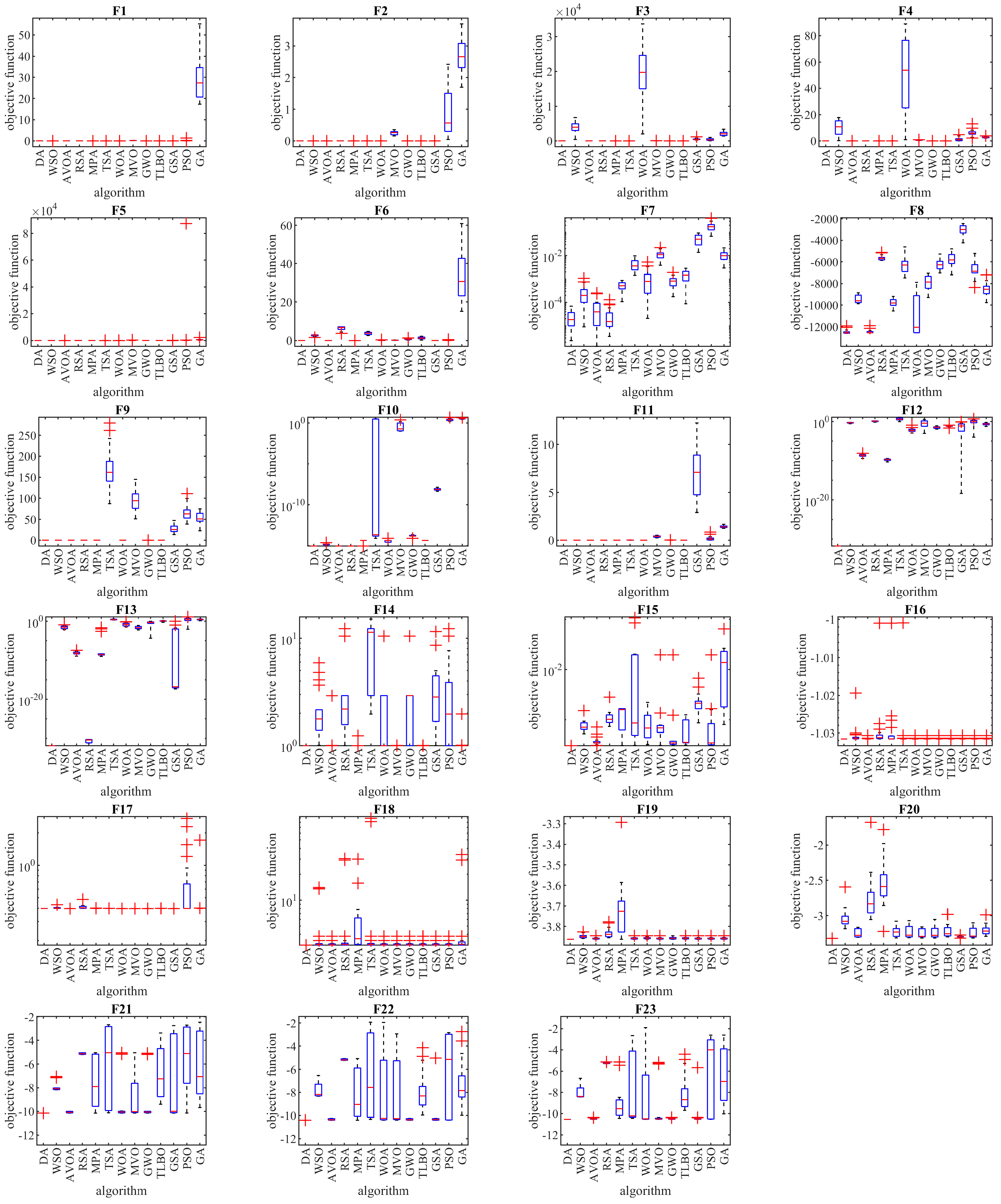
3.1. Evaluation of Unimodal Functions
3.2. Evaluation of High-Dimensional Multimodal Functions
3.3. Evaluation of Fixed-Dimensional Multimodal Functions
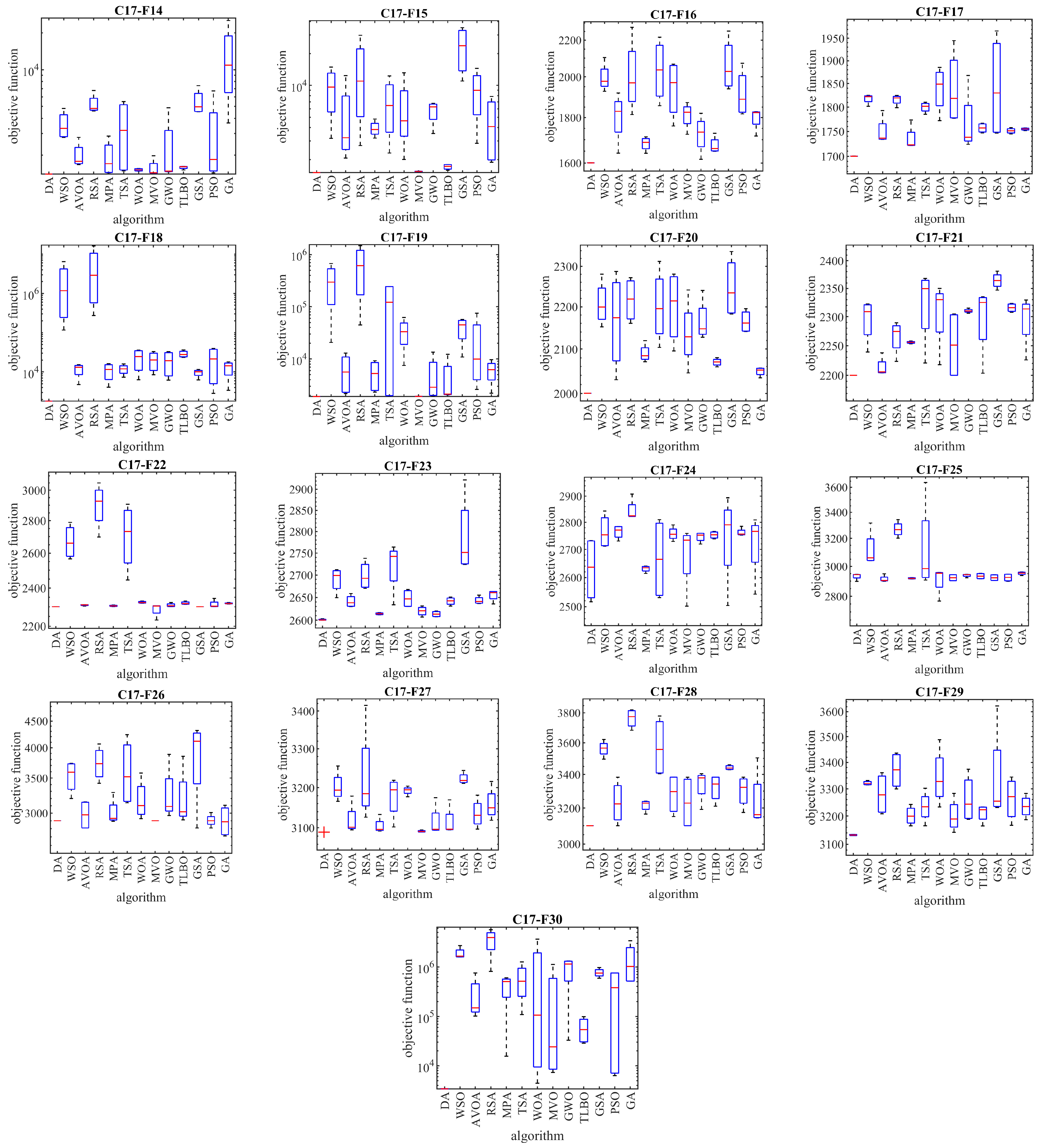
3.4. Evaluation of the CEC 2017 Test Suite
3.5. Statistical Analysis
4. DA for Real-World Applications
5. Conclusions and Future Works
Author Contributions
Funding
Institutional Review Board Statement
Data Availability Statement
Acknowledgments
Conflicts of Interest
References
- Clerc, M. Particle Swarm Optimization; Wiley-ISTE: London, UK, 2006. [Google Scholar]
- Yang, X.-S. Nature-Inspired Algorithms and Applied Optimization; Springer International Publishing AG: New York, NY, USA, 2017. [Google Scholar]
- Iba, K. Reactive power optimization by genetic algorithm. IEEE Trans. Power Syst. 1994, 9, 685–692. [Google Scholar] [CrossRef]
- Mirjalili, S.; Sadiq, A.S. Magnetic Optimization Algorithm for training Multi Layer Perceptron. In Proceedings of the 2011 IEEE 3rd International Conference on Communication Software and Networks, Xi’an, China, 27–29 May 2011; pp. 42–46. [Google Scholar]
- Mirjalili, S.; Hashim, S.Z.M.; Sardroudi, H.M. Training feedforward neural networks using hybrid particle swarm optimization and gravitational search algorithm. Appl. Math. Comput. 2012, 218, 11125–11137. [Google Scholar] [CrossRef]
- Yi, N.; Xu, J.; Yan, L.; Huang, L. Task optimization and scheduling of distributed cyber–physical system based on improved ant colony algorithm. Future Gener. Comput. Syst. 2020, 109, 134–148. [Google Scholar] [CrossRef]
- Rezk, H.; Fathy, A.; Aly, M.; Ibrahim, M.N.F. Energy management control strategy for renewable energy system based on spotted hyena optimizer. Comput. Mater. Contin. 2021, 67, 2271–2281. [Google Scholar] [CrossRef]
- Akbari, E.; Ghasemi, M.; Gil, M.; Rahimnejad, A.; Gadsden, S.A. Optimal Power Flow via Teaching-Learning-Studying-Based Optimization Algorithm. Electr. Power Compon. Syst. 2021, 49, 584–601. [Google Scholar] [CrossRef]
- Adhvaryyu, P.K.; Chattopadhyay, P.K.; Bhattacharjya, A. Application of bio-inspired krill herd algorithm to combined heat and power economic dispatch. In Proceedings of the 2014 IEEE Innovative Smart Grid Technologies—Asia (ISGT ASIA), Kuala Lumpur, Malaysia, 20–23 May 2014; pp. 338–343. [Google Scholar]
- Panda, M.; Nayak, Y.K. Impact analysis of renewable energy Distributed Generation in deregulated electricity markets: A context of Transmission Congestion Problem. Energy 2022, 254, 124403. [Google Scholar] [CrossRef]
- Kottath, R.; Singh, P. Influencer buddy optimization: Algorithm and its application to electricity load and price forecasting problem. Energy 2023, 263, 125641. [Google Scholar] [CrossRef]
- Xing, Z.; Zhu, J.; Zhang, Z.; Qin, Y.; Jia, L. Energy consumption optimization of tramway operation based on improved PSO algorithm. Energy 2022, 258, 124848. [Google Scholar] [CrossRef]
- Montazeri, Z.; Niknam, T. Optimal utilization of electrical energy from power plants based on final energy consumption using gravitational search algorithm. Electr. Eng. Electromechanics 2018, 4, 70–73. [Google Scholar] [CrossRef] [Green Version]
- Song, Y.H.; Xuan, Q.Y. Combined heat and power economic dispatch using genetic algorithm based penalty function method. Electr. Mach. Power Syst. 1998, 26, 363–372. [Google Scholar] [CrossRef]
- Premkumar, M.; Sowmya, R.; Jangir, P.; Nisar, K.S.; Aldhaifallah, M. A new metaheuristic optimization algorithms for brushless direct current wheel motor design problem. CMC Comput. Mater. Contin. 2021, 67, 2227–2242. [Google Scholar] [CrossRef]
- Carbas, S.; Toktas, A.; Ustun, D. Nature-Inspired Metaheuristic Algorithms for Engineering Optimization Appzlications; Springer: New York, NY, USA, 2021. [Google Scholar]
- Yang, X.-S. Optimization and metaheuristic algorithms in engineering. In Metaheuristics in Water, Geotechnical and Transport Engineering; Elsevier: Amsterdam, The Netherlands, 2013; pp. 1–23. [Google Scholar]
- Kennedy, J.; Eberhart, R. Particle swarm optimization. In Proceedings of the ICNN’95—International Conference on Neural Networks, Perth, WA, Australia, 27 November–1 December 1995; Volume 4, pp. 1942–1948. [Google Scholar]
- Dorigo, M.; Maniezzo, V.; Colorni, A. Ant system: Optimization by a colony of cooperating agents. IEEE Trans. Syst. Man Cybern. Part B 1996, 26, 29–41. [Google Scholar] [CrossRef] [Green Version]
- Karaboga, D.; Basturk, B. A powerful and efficient algorithm for numerical functionoptimization: Artificial bee colony (ABC) algorithm. J. Glob. Optim. 2007, 39, 459–471. [Google Scholar] [CrossRef]
- Gandomi, A.H.; Alavi, A.H. Krill herd: A new bio-inspired optimization algorithm. Commun. Nonlinear Sci. Numer. Simul. 2012, 17, 4831–4845. [Google Scholar] [CrossRef]
- Mirjalili, S.; Mirjalili, S.M.; Lewis, A. Grey wolf optimizer. Adv. Eng. Softw. 2014, 69, 46–61. [Google Scholar] [CrossRef] [Green Version]
- Chen, Z.; Francis, A.; Li, S.; Liao, B.; Xiao, D.; Ha, T.T.; Li, J.; Ding, L.; Cao, X. Egret Swarm Optimization Algorithm: An Evolutionary Computation Approach for Model Free Optimization. Biomimetics 2022, 7, 144. [Google Scholar] [CrossRef]
- Khan, A.H.; Cao, X.; Xu, B.; Li, S. Beetle antennae search: Using biomimetic foraging behaviour of beetles to fool a well-trained neuro-intelligent system. Biomimetics 2022, 7, 84. [Google Scholar] [CrossRef]
- Dehghani, M.; Trojovský, P. Serval Optimization Algorithm: A New Bio-Inspired Approach for Solving Optimization Problems. Biomimetics 2022, 7, 204. [Google Scholar] [CrossRef]
- Trojovský, P.; Dehghani, M. Subtraction-Average-Based Optimizer: A New Swarm-Inspired Metaheuristic Algorithm for Solving Optimization Problems. Biomimetics 2023, 8, 149. [Google Scholar] [CrossRef]
- Faramarzi, A.; Heidarinejad, M.; Mirjalili, S.; Gandomi, A.H. Marine predators algorithm: A nature-inspired metaheuristic. Expert Syst. Appl. 2020, 152, 113377. [Google Scholar] [CrossRef]
- Dehghani, M.; Montazeri, Z.; Trojovská, E.; Trojovský, P. Coati Optimization Algorithm: A new bio-inspired metaheuristic algorithm for solving optimization problems. Knowl. Based Syst. 2023, 259, 110011. [Google Scholar] [CrossRef]
- Kaur, S.; Awasthi, L.K.; Sangal, A.L.; Dhiman, G. Tunicate swarm algorithm: A new bio-inspired based metaheuristic paradigm for global optimization. Eng. Appl. Artif. Intell. 2020, 90, 103541. [Google Scholar] [CrossRef]
- Kaveh, M.; Mesgari, M.S.; Saeidian, B. Orchard Algorithm (OA): A new meta-heuristic algorithm for solving discrete and continuous optimization problems. Math. Comput. Simul. 2023, 208, 95–135. [Google Scholar] [CrossRef]
- Cuevas, E.; Cienfuegos, M.; Zaldívar, D.; Pérez-Cisneros, M. A swarm optimization algorithm inspired in the behavior of the social-spider. Expert Syst. Appl. 2013, 40, 6374–6384. [Google Scholar] [CrossRef] [Green Version]
- Dhiman, G.; Kumar, V. Emperor penguin optimizer: A bio-inspired algorithm for engineering problems. Knowl. Based Syst. 2018, 159, 20–50. [Google Scholar] [CrossRef]
- Yazdani, M.; Jolai, F. Lion Optimization Algorithm (LOA): A nature-inspired metaheuristic algorithm. J. Comput. Des. Eng. 2016, 3, 24–36. [Google Scholar] [CrossRef] [Green Version]
- Yang, X.S.; Deb, S. Engineering optimisation by cuckoo search. Int. J. Math. Model. Numer. Optim. 2010, 1, 330–343. [Google Scholar] [CrossRef]
- Dehghani, M.; Trojovský, P.; Malik, O.P. Green Anaconda Optimization: A New Bio-Inspired Metaheuristic Algorithm for Solving Optimization Problems. Biomimetics 2023, 8, 121. [Google Scholar] [CrossRef]
- Doumari, S.A.; Givi, H.; Dehghani, M.; Montazeri, Z.; Leiva, V.; Guerrero, J.M. A new two-stage algorithm for solving optimization problems. Entropy 2021, 23, 491. [Google Scholar] [CrossRef]
- Zhao, W.; Zhang, Z.; Wang, L. Manta ray foraging optimization: An effective bio-inspired optimizer for engineering applications. Eng. Appl. Artif. Intell. 2020, 87, 103300. [Google Scholar] [CrossRef]
- Abdollahzadeh, B.; Gharehchopogh, F.S.; Khodadadi, N.; Mirjalili, S. Mountain Gazelle Optimizer: A new Nature-inspired Metaheuristic Algorithm for Global Optimization Problems. Adv. Eng. Softw. 2022, 174, 103282. [Google Scholar] [CrossRef]
- Shen, C.; Zhang, K. Two-stage improved Grey Wolf optimization algorithm for feature selection on high-dimensional classification. Complex Intell. Syst. 2022, 8, 2769–2789. [Google Scholar] [CrossRef]
- Goldberg, D.E.; Holland, J.H. Genetic algorithms and machine learning. Mach. Learn. 1988, 3, 95–99. [Google Scholar] [CrossRef]
- Beyer, H.G.; Schwefel, H.P. Evolution strategies—A comprehensive introduction. Nat. Comput. 2002, 1, 3–52. [Google Scholar] [CrossRef]
- Simon, D. Biogeography-based optimization. IEEE Trans. Evol. Comput. 2008, 12, 702–713. [Google Scholar] [CrossRef] [Green Version]
- Banzhaf, W.; Nordin, P.; Keller, R.E.; Francone, F.D. Genetic Programming: An Introduction; Morgan Kaufmann Publishers: San Francisco, CA, USA, 1998; Volume 1. [Google Scholar]
- Storn, R.; Price, K. Differential evolution—A simple and efficient heuristic for global optimization over continuous spaces. J. Glob. Optim. 1997, 11, 341–359. [Google Scholar] [CrossRef]
- Rashedi, E.; Nezamabadi-Pour, H.; Saryazdi, S. GSA: A gravitational search algorithm. Inf. Sci. 2009, 179, 2232–2248. [Google Scholar] [CrossRef]
- Ghasemi, M.; Davoudkhani, I.F.; Akbari, E.; Rahimnejad, A.; Ghavidel, S.; Li, L. A novel and effective optimization algorithm for global optimization and its engineering applications: Turbulent Flow of Water-based Optimization (TFWO). Eng. Appl. Artif. Intell. 2022, 92, 103666. [Google Scholar] [CrossRef]
- Kaveh, A.; Dadras, A. A novel meta-heuristic optimization algorithm: Thermal exchange optimization. Adv. Eng. Softw. 2017, 110, 69–84. [Google Scholar] [CrossRef]
- Shah-Hosseini, H. Principal components analysis by the galaxy-based search algorithm: A novel metaheuristic for continuous optimisation. Int. J. Comput. Sci. Eng. 2011, 6, 132–140. [Google Scholar]
- Hatamlou, A. Black hole: A new heuristic optimization approach for data clustering. Inf. Sci. 2013, 222, 175–184. [Google Scholar] [CrossRef]
- Kaveh, A.; Khayatazad, M. A new meta-heuristic method: Ray optimization. Comput. Struct. 2012, 112–113, 283–294. [Google Scholar] [CrossRef]
- Erol, O.K.; Eksin, I. A new optimization method: Big Bang–Big Crunch. Adv. Eng. Softw. 2006, 37, 106–111. [Google Scholar] [CrossRef]
- Du, H.; Wu, X.; Zhuang, J. Small-world optimization algorithm for function optimization. In Advances in Natural Computation; Jiao, L., Wang, L., Gao, X., Liu, J., Wu, F., Eds.; Springer: Berlin/Heidelberg, Germany, 2006; pp. 264–273. [Google Scholar]
- Tayarani-N, M.H.; Akbarzadeh-T, M.R. Magnetic optimization algorithms a new synthesis. In Proceedings of the Congress on Evolutionary Computation (IEEE World Congress on Computational Intelligence), Hong Kong, China, 1–6 June 2008; pp. 2659–2664. [Google Scholar]
- Alatas, B. ACROA: Artificial chemical reaction optimization algorithm for global optimization. Expert Syst. Appl. 2011, 38, 13170–13180. [Google Scholar] [CrossRef]
- Kashan, A.H. League Championship Algorithm (LCA): An algorithm for global optimization inspired by sport championships. Appl. Soft Comput. 2014, 16, 171–200. [Google Scholar] [CrossRef]
- Dehghani, M.; Mardaneh, M.; Guerrero, J.M.; Malik, O.; Kumar, V. Football game based optimization: An application to solve energy commitment problem. Int. J. Intell. Eng. Syst. 2020, 13, 514–523. [Google Scholar] [CrossRef]
- Moghdani, R.; Salimifard, K. Volleyball Premier League Algorithm. Appl. Soft Comput. 2018, 64, 161–185. [Google Scholar] [CrossRef]
- Subramaniyan, S.; Ramiah, J. Improved football game optimization for state estimation and power quality enhancement. Comput. Electr. Eng. 2020, 81, 106547. [Google Scholar] [CrossRef]
- Ma, B.; Hu, Y.; Pengmin Lu, P.; Liu, Y. Running city game optimizer: A game-based metaheuristic optimization algorithm for global optimization. J. Comput. Des. Eng. 2023, 10, 65–107. [Google Scholar] [CrossRef]
- Xu, S.; Chen, H. Nash game based efficient global optimization for large-scale design problems. J. Glob. Optim. 2018, 71, 361–381. [Google Scholar] [CrossRef]
- Srilakshmi, K.; Babu, P.R.; Venkatesan, Y.; Palanivelu, A. Soccer league optimization for load flow analysis of power systems. Int. J. Numer. Model. Electron. Netw. Devices Fields 2021, 35, e2965. [Google Scholar] [CrossRef]
- Rao, R.V.; Savsani, V.J.; Vakharia, D. Teaching–learning-based optimization: A novel method for constrained mechanical design optimization problems. Comput. Aided Des. 2011, 43, 303–315. [Google Scholar] [CrossRef]
- Dehghani, M.; Mardaneh, M.; Guerrero, J.M.; Malik, O.P.; Ramirez-Mendoza, R.A.; Matas, J.; Vasquez, J.C.; Parra-Arroyo, L. A new “Doctor and Patient” optimization algorithm: An application to energy commitment problem. Appl. Sci. 2020, 10, 5791. [Google Scholar] [CrossRef]
- Trojovský, P.; Dehghani, M. A new optimization algorithm based on mimicking the voting process for leader selection. PeerJ Comput. Sci. 2022, 8, e976. [Google Scholar] [CrossRef]
- Dehghani, M.; Trojovský, P. Teamwork Optimization Algorithm: A New Optimization Approach for Function Minimization/Maximization. Sensors 2021, 21, 4567. [Google Scholar] [CrossRef]
- Dehghani, M.; Trojovská, E.; Trojovský, P. A new human-based metaheuristic algorithm for solving optimization problems on the base of simulation of driving training process. Sci. Rep. 2022, 12, 9924. [Google Scholar] [CrossRef]
- Zeidabadi, F.-A.; Dehghani, M.; Trojovský, P.; Hubálovský, Š.; Leiva, V.; Dhiman, G. Archery Algorithm: A Novel Stochastic Optimization Algorithm for Solving Optimization Problems. Comput. Mater. Contin. 2022, 72, 399–416. [Google Scholar] [CrossRef]
- Dehghani, M.; Montazeri, Z.; Dehghani, A.; Malik, O.P. GO: Group optimization. Gazi Univ. J. Sci. 2020, 33, 381–392. [Google Scholar] [CrossRef]
- Dehghani, M.; Mardaneh, M.; Malik, O. FOA: ‘Following’Optimization Algorithm for solving Power engineering optimization problems. J. Oper. Autom. Power Eng. 2020, 8, 57–64. [Google Scholar]
- Wolpert, D.H.; Macready, W.G. No free lunch theorems for optimization. IEEE Trans. Evol. Comput. 1997, 1, 67–82. [Google Scholar] [CrossRef] [Green Version]
- Awad, N.; Ali, M.; Liang, J.; Qu, B.; Suganthan, P.N. Problem Definitions and Evaluation Criteria for the CEC 2017 Special Session and Competition on Single Objective Real-Parameter Numerical Optimization; Technical Report; Nanyang Technological University: Singapore, 2016. [Google Scholar]
- Wilcoxon, F. Individual comparisons by ranking methods. In Breakthroughs in Statistics; Springer: New York, NY, USA, 1992; pp. 196–202. [Google Scholar]
- Das, S.; Suganthan, P.N. Problem Definitions and Evaluation Criteria for CEC 2011 Competition on Testing Evolutionary Algorithms on Real World Optimization Problems. Technical Reports. 2010. Available online: al-roomi.org/multimedia/CEC_Database/CEC2011/CEC2011_TechnicalReport.pdf (accessed on 4 June 2023).


| Algorithm | Parameter | Value |
|---|---|---|
| GA | Type | Real coded |
| Selection | Roulette wheel (proportionate) | |
| Crossover | Whole arithmetic (, ) | |
| Mutation | Gaussian () | |
| PSO | Topology | Fully connected |
| Cognitive and social constant | ||
| Inertia weight | Linear reduction from 0.9 to 0.1 | |
| Velocity limit | 10% of dimension range | |
| GSA | Alpha, | 20, 100, 2, 1 |
| TLBO | : teaching factor | |
| Random number | is a random number between | |
| GWO | Convergence parameter () | : Linear reduction from 2 to 0 |
| MVO | Wormhole existence probability (WEP) | and |
| Exploitation accuracy over the iterations () | ||
| WOA | Convergence parameter (a) | a: Linear reduction from 2 to 0 |
| is a random vector in | ||
| is a random number in | ||
| TSA | and | 1, 4 |
| Random numbers lie in the range of . | ||
| MPA | Constant number | |
| Random vector | R is a vector of uniform random numbers in | |
| Fish aggregating devices (FADs) | ||
| Binary vector | or 1 | |
| RSA | Sensitive parameter | |
| Sensitive parameter | ||
| Evolutionary sense (ES) | ES: randomly decreasing values between 2 and | |
| AVOA | 0.8, 0.2 | |
| w | 2.5 | |
| 0.6, 0.4, 0.6 | ||
| WSO | and | 0.07, 0.75 |
| 4.125, 6.25, 100, 0.0005 |
| DA | WSO | AVOA | RSA | MPA | TSA | WOA | MVO | GWO | TLBO | GSA | PSO | GA | ||
|---|---|---|---|---|---|---|---|---|---|---|---|---|---|---|
| F1 | mean | 0 | 2.70 × 10−152 | 0 | 0 | 1.86 × 10−49 | 4.51 × 10−47 | 1.30 × 10−151 | 0.145162 | 1.72 × 10−59 | 2.45 × 10−74 | 1.29 × 10⁻¹⁶ | 0.097939 | 29.59 |
| best | 0 | 1.80 × 10−171 | 0 | 0 | 3.69 × 10−52 | 1.40 × 10−50 | 9.10 × 10−171 | 0.102355 | 1.45 × 10−61 | 5.69 × 10−77 | 5.20 × 10⁻¹⁷ | 4.72 × 10⁻⁴ | 17.39095 | |
| worst | 0 | 5.20 × 10−151 | 0 | 0 | 1.61 × 10−48 | 3.21 × 10−46 | 2.60 × 10−150 | 0.195279 | 7.48 × 10−59 | 2.52 × 10−73 | 3.63 × 10⁻¹⁶ | 1.355952 | 55.22585 | |
| std | 0 | 1.30 × 10−151 | 0 | 0 | 4.20 × 10−49 | 1.07 × 10−46 | 6.40 × 10−151 | 0.029675 | 2.29 × 10−59 | 6.58 × 10−74 | 7.65 × 10⁻¹⁷ | 0.332239 | 11.18532 | |
| median | 0 | 4.20 × 10−160 | 0 | 0 | 4.04 × 10−50 | 4.15 × 10−48 | 2.10 × 10−159 | 0.146027 | 1.04 × 10−59 | 1.64 × 10−75 | 1.10 × 10⁻¹⁶ | 0.009429 | 27.35582 | |
| rank | 1 | 2 | 1 | 1 | 6 | 7 | 3 | 10 | 5 | 4 | 8 | 9 | 11 | |
| F2 | mean | 0 | 4.90 × 10−106 | 1.10 × 10−276 | 0 | 6.76 × 10⁻²⁸ | 2.05 × 10⁻²⁸ | 2.40 × 10−105 | 0.251424 | 1.31 × 10⁻³⁴ | 6.56 × 10−39 | 5.32 × 10⁻⁸ | 0.86873 | 2.705022 |
| best | 0 | 1.50 × 10−118 | 1.30 × 10−306 | 0 | 1.79 × 10⁻²⁹ | 1.96 × 10⁻³⁰ | 7.70 × 10−118 | 0.155288 | 4.72 × 10−36 | 8.56 × 10−40 | 3.38 × 10⁻⁸ | 0.043928 | 1.69317 | |
| worst | 0 | 5.30 × 10−105 | 2.10 × 10−275 | 0 | 4.57 × 10⁻²⁷ | 1.77 × 10⁻²⁷ | 2.70 × 10−104 | 0.353611 | 7.67 × 10⁻³⁴ | 2.37 × 10−38 | 1.20 × 10⁻⁷ | 2.418765 | 3.69274 | |
| std | 0 | 1.50 × 10−105 | 0 | 0 | 1.17 × 10⁻²⁷ | 5.66 × 10⁻²⁸ | 7.40 × 10−105 | 0.067341 | 2.09 × 10⁻³⁴ | 5.97 × 10−39 | 2.00 × 10⁻⁸ | 0.772627 | 0.582406 | |
| median | 0 | 6.70 × 10−109 | 6.30 × 10−290 | 0 | 3.41 × 10⁻²⁸ | 1.92 × 10⁻²⁹ | 3.30 × 10−108 | 0.260325 | 6.31 × 10⁻³⁵ | 4.83 × 10−39 | 4.98 × 10⁻⁸ | 0.566698 | 2.659583 | |
| rank | 1 | 3 | 2 | 1 | 8 | 7 | 4 | 10 | 6 | 5 | 9 | 11 | 12 | |
| F3 | mean | 0 | 3872.488 | 0 | 0 | 2.44 × 10⁻¹² | 1.15 × 10⁻¹⁰ | 19362.44 | 15.49573 | 2.11 × 10⁻¹⁴ | 3.73 × 10⁻²⁴ | 461.2824 | 376.5264 | 2104.13 |
| best | 0 | 400.6281 | 0 | 0 | 6.00 × 10⁻¹⁹ | 1.33 × 10⁻²¹ | 2003.141 | 5.795644 | 2.29 × 10⁻¹⁹ | 2.13 × 10⁻²⁹ | 238.6095 | 21.11739 | 1381.604 | |
| worst | 0 | 6730.25 | 0 | 0 | 1.39 × 10⁻¹¹ | 1.89 × 10⁻⁹ | 33651.25 | 47.47647 | 3.92 × 10⁻¹³ | 3.50 × 10⁻²³ | 1150.846 | 994.7339 | 3355.513 | |
| std | 0 | 1829.604 | 0 | 0 | 4.69 × 10⁻¹² | 4.66 × 10⁻¹⁰ | 9148.022 | 11.50818 | 9.64 × 10⁻¹⁴ | 1.16 × 10⁻²³ | 235.4943 | 308.3468 | 683.8623 | |
| median | 0 | 3943.313 | 0 | 0 | 1.77 × 10⁻¹³ | 1.04 × 10⁻¹³ | 19,716.57 | 11.52407 | 4.52 × 10⁻¹⁶ | 3.92 × 10⁻²⁶ | 388.3647 | 284.2824 | 2037.889 | |
| rank | 1 | 10 | 1 | 1 | 4 | 5 | 11 | 6 | 3 | 2 | 8 | 7 | 9 | |
| F4 | mean | 0 | 10.05438 | 3.10 × 10−265 | 0 | 2.89 × 10⁻¹⁹ | 0.004291 | 50.27188 | 0.530759 | 1.19 × 10⁻¹⁴ | 1.78 × 10⁻³⁰ | 1.198928 | 6.092114 | 2.744796 |
| best | 0 | 0.175505 | 0 | 0 | 2.93 × 10⁻²⁰ | 9.37 × 10⁻⁵ | 0.877525 | 0.257974 | 6.36 × 10⁻¹⁶ | 5.64 × 10⁻³² | 9.60 × 10⁻⁹ | 2.221789 | 2.150196 | |
| worst | 0 | 17.79352 | 4.40 × 10−264 | 0 | 9.32 × 10⁻¹⁹ | 0.034756 | 88.96761 | 0.934252 | 5.57 × 10⁻¹⁴ | 7.88 × 10⁻³⁰ | 4.780357 | 12.96077 | 3.873355 | |
| std | 0 | 6.331918 | 0 | 0 | 2.45 × 10⁻¹⁹ | 0.008493 | 31.65959 | 0.20548 | 1.56 × 10⁻¹⁴ | 2.56 × 10⁻³⁰ | 1.482929 | 2.675169 | 0.499179 | |
| median | 0 | 10.75345 | 1.90 × 10−282 | 0 | 2.51 × 10⁻¹⁹ | 0.001426 | 53.76726 | 0.515167 | 6.16 × 10⁻¹⁵ | 6.33 × 10⁻³¹ | 0.87983 | 5.706585 | 2.700252 | |
| rank | 1 | 11 | 2 | 1 | 4 | 6 | 12 | 7 | 5 | 3 | 8 | 10 | 9 | |
| F5 | mean | 0 | 10.34262 | 1.39 × 10⁻⁵ | 12.60997 | 22.6266 | 27.62587 | 26.49314 | 93.34453 | 25.7868 | 25.98698 | 42.73281 | 4474.037 | 577.5834 |
| best | 0 | 5.208632 | 1.35 × 10⁻⁶ | 8.44 × 10⁻²⁹ | 22.12664 | 24.90348 | 25.92307 | 26.80555 | 24.80211 | 24.82359 | 25.11065 | 25.49519 | 221.9666 | |
| worst | 0 | 16.82213 | 5.73 × 10⁻⁵ | 28.12341 | 23.3302 | 28.02781 | 27.87618 | 366.6048 | 26.34408 | 27.89297 | 162.2436 | 87,383.97 | 2189.572 | |
| std | 0 | 6.306277 | 1.55 × 10⁻⁵ | 15.76275 | 0.415468 | 0.84255 | 0.617609 | 108.4702 | 0.562673 | 1.000998 | 47.38394 | 21,505.67 | 454.3321 | |
| median | 0 | 5.493341 | 9.10 × 10⁻⁶ | 1.19 × 10⁻²⁸ | 22.59841 | 27.96078 | 26.27693 | 29.12051 | 25.44735 | 25.54065 | 25.55866 | 83.52371 | 461.3534 | |
| rank | 1 | 3 | 2 | 4 | 5 | 9 | 8 | 11 | 6 | 7 | 10 | 13 | 12 | |
| F6 | mean | 0 | 2.521744 | 4.83 × 10⁻⁸ | 6.264793 | 1.75 × 10⁻⁹ | 3.571818 | 0.079134 | 0.146488 | 0.64109 | 1.223689 | 1.02 × 10⁻¹⁶ | 0.061549 | 33.12645 |
| best | 0 | 1.427146 | 6.90 × 10⁻⁹ | 3.553726 | 7.84 × 10⁻¹⁰ | 2.476483 | 0.010206 | 0.076864 | 0.239352 | 0.226151 | 5.36 × 10⁻¹⁷ | 1.85 × 10⁻⁶ | 15.14563 | |
| worst | 0 | 2.876686 | 1.32 × 10⁻⁷ | 7.033228 | 4.66 × 10⁻⁹ | 4.644524 | 0.316978 | 0.242632 | 1.214835 | 2.100066 | 1.75 × 10⁻¹⁶ | 0.525533 | 60.89028 | |
| std | 0 | 0.435018 | 3.51 × 10⁻⁸ | 1.098922 | 1.00 × 10⁻⁹ | 0.741235 | 0.108637 | 0.050652 | 0.327781 | 0.531559 | 3.97 × 10⁻¹⁷ | 0.158821 | 14.48562 | |
| median | 0 | 2.674209 | 4.47 × 10⁻⁸ | 6.679094 | 1.55 × 10⁻⁹ | 3.682495 | 0.030662 | 0.155367 | 0.705569 | 1.181024 | 9.19 × 10⁻¹⁷ | 0.001996 | 30.73489 | |
| rank | 1 | 10 | 4 | 12 | 3 | 11 | 6 | 7 | 8 | 9 | 2 | 5 | 13 | |
| F7 | mean | 2.54 × 10⁻⁵ | 2.85 × 10⁻⁴ | 6.14 × 10⁻⁵ | 2.99 × 10⁻⁵ | 0.000531 | 0.004214 | 0.001241 | 0.011268 | 0.000807 | 0.001485 | 0.051231 | 0.178636 | 0.010273 |
| best | 2.35 × 10⁻⁶ | 9.02 × 10⁻⁶ | 1.34 × 10⁻⁶ | 3.49 × 10⁻⁶ | 0.000108 | 0.001449 | 2.07 × 10⁻⁵ | 0.003853 | 0.000177 | 8.77 × 10⁻⁵ | 0.013704 | 0.066954 | 0.002942 | |
| worst | 6.89 × 10⁻⁵ | 0.001072 | 0.000256 | 0.000129 | 0.000873 | 0.009676 | 0.005238 | 0.021895 | 0.001899 | 0.002859 | 0.092717 | 0.399054 | 0.021284 | |
| std | 2.18 × 10⁻⁵ | 3.09 × 10⁻⁴ | 7.84 × 10⁻⁵ | 3.69 × 10⁻⁵ | 0.00023 | 0.002503 | 0.001545 | 0.005381 | 0.000499 | 0.00094 | 0.026681 | 0.084471 | 0.005152 | |
| median | 1.83 × 10⁻⁵ | 2.00 × 10⁻⁴ | 3.95 × 10⁻⁵ | 1.51 × 10⁻⁵ | 0.000518 | 0.003611 | 0.000794 | 0.010978 | 0.00082 | 0.001462 | 0.050284 | 0.172417 | 0.009875 | |
| rank | 1 | 4 | 3 | 2 | 5 | 9 | 7 | 11 | 6 | 8 | 12 | 13 | 10 | |
| Sum rank | 7 | 43 | 15 | 22 | 35 | 54 | 51 | 62 | 39 | 38 | 57 | 68 | 76 | |
| Mean rank | 1 | 6.1428571 | 2.1428571 | 3.1428571 | 5 | 7.7142857 | 7.2857143 | 8.8571429 | 5.5714286 | 5.4285714 | 8.1428571 | 9.7142857 | 10.857143 | |
| Total rank | 1 | 7 | 2 | 3 | 4 | 9 | 8 | 11 | 6 | 5 | 10 | 12 | 13 | |
| DA | WSO | AVOA | RSA | MPA | TSA | WOA | MVO | GWO | TLBO | GSA | PSO | GA | ||
|---|---|---|---|---|---|---|---|---|---|---|---|---|---|---|
| F8 | mean | −12,498.587 | −9469.161 | −12,471.545 | −5647.3779 | −9771.5065 | −6329.3267 | −11,107.96 | −7972.4501 | −6271.5652 | −5804.7042 | −3071.8049 | −6725.3549 | −8543.4031 |
| best | −12,622.812 | −9866.2622 | −12,571.081 | −5864.3072 | −10,538.388 | −7476.6259 | −12,569.905 | −9290.7597 | −7026.1104 | −7194.9064 | −4232.9513 | −8358.1095 | −9767.7805 | |
| worst | −11,936.272 | −8854.7341 | −11,917.074 | −5130.8349 | −9190.6957 | −4611.0881 | −7883.2501 | −7049.8979 | −5274.2783 | −4791.287 | −2440.9757 | −5216.7278 | −7194.9171 | |
| std | 209.81989 | 395.93068 | 208.38669 | 240.75731 | 395.20999 | 781.55525 | 1854.4961 | 780.48164 | 511.88428 | 652.44489 | 532.29246 | 797.42343 | 685.87708 | |
| median | −12,577.838 | −9593.2117 | −12,568.073 | −5693.4379 | −9800.0269 | −6292.0143 | −12,056.375 | −7854.7623 | −6267.6723 | −5820.1694 | −2989.8155 | −6867.7852 | −8524.8117 | |
| rank | 1 | 5 | 2 | 12 | 4 | 9 | 3 | 7 | 10 | 11 | 13 | 8 | 6 | |
| F9 | mean | 0 | 0 | 0 | 0 | 0 | 167.94776 | 0 | 94.904612 | 1.654 × 10⁻¹⁴ | 0 | 27.653242 | 65.689736 | 53.046261 |
| best | 0 | 0 | 0 | 0 | 0 | 87.061474 | 0 | 51.208516 | 0 | 0 | 13.512937 | 38.60839 | 22.537741 | |
| worst | 0 | 0 | 0 | 0 | 0 | 279.5677 | 0 | 144.81711 | 1.103 × 10⁻¹³ | 0 | 47.295235 | 111.13666 | 74.601525 | |
| std | 0 | 0 | 0 | 0 | 0 | 54.529301 | 0 | 26.93684 | 3.471 × 10⁻¹⁴ | 0 | 9.7990172 | 20.142107 | 14.760996 | |
| median | 0 | 0 | 0 | 0 | 0 | 161.69195 | 0 | 94.18019 | 0 | 0 | 25.578047 | 63.123014 | 51.041263 | |
| rank | 1 | 1 | 1 | 1 | 1 | 7 | 1 | 6 | 2 | 1 | 3 | 5 | 4 | |
| F10 | mean | 8.88 × 10⁻¹⁶ | 1.509 × 10⁻¹⁵ | 8.88 × 10⁻¹⁶ | 8.88 × 10⁻¹⁶ | 4.16 × 10⁻¹⁵ | 1.2053421 | 3.99 × 10⁻¹⁵ | 0.5606201 | 1.62 × 10⁻¹⁴ | 4.33 × 10⁻¹⁵ | 7.97 × 10⁻⁹ | 2.6456892 | 3.4682044 |
| best | 8.88 × 10⁻¹⁶ | 8.882 × 10⁻¹⁶ | 8.88 × 10⁻¹⁶ | 8.88 × 10⁻¹⁶ | 8.88 × 10⁻¹⁶ | 7.78 × 10⁻¹⁵ | 8.88 × 10⁻¹⁶ | 0.0975925 | 7.78 × 10⁻¹⁵ | 4.33 × 10⁻¹⁵ | 4.52 × 10⁻⁹ | 1.6428153 | 2.7957914 | |
| worst | 8.88 × 10⁻¹⁶ | 2.267 × 10⁻¹⁵ | 8.88 × 10⁻¹⁶ | 8.88 × 10⁻¹⁶ | 4.33 × 10⁻¹⁵ | 3.2725869 | 7.78 × 10⁻¹⁵ | 2.4399845 | 2.16 × 10⁻¹⁴ | 4.33 × 10⁻¹⁵ | 1.40 × 10⁻⁸ | 4.9058652 | 4.5031721 | |
| std | 0 | 4.867 × 10⁻¹⁶ | 0 | 0 | 8.493 × 10⁻¹⁶ | 1.6778805 | 2.43 × 10⁻¹⁵ | 0.7239449 | 3.79 × 10⁻¹⁵ | 8.92 × 10⁻³¹ | 2.50 × 10⁻⁹ | 0.9170296 | 0.4240318 | |
| median | 8.88 × 10⁻¹⁶ | 1.577 × 10⁻¹⁵ | 8.88 × 10⁻¹⁶ | 8.88 × 10⁻¹⁶ | 4.33 × 10⁻¹⁵ | 2.16 × 10⁻¹⁴ | 4.33 × 10⁻¹⁵ | 0.1885052 | 1.47 × 10⁻¹⁴ | 4.33 × 10⁻¹⁵ | 7.49 × 10⁻⁹ | 2.6521765 | 3.5210558 | |
| rank | 1 | 2 | 1 | 1 | 4 | 9 | 3 | 8 | 6 | 5 | 7 | 10 | 11 | |
| F11 | mean | 0 | 0 | 0 | 0 | 0 | 0.0085784 | 0 | 0.387725 | 0.0012996 | 0 | 6.9924949 | 0.1797264 | 1.4294144 |
| best | 0 | 0 | 0 | 0 | 0 | 0 | 0 | 0.246549 | 0 | 0 | 2.906073 | 0.0022963 | 1.2495814 | |
| worst | 0 | 0 | 0 | 0 | 0 | 0.0199327 | 0 | 0.51996 | 0.0182608 | 0 | 12.259906 | 0.8496609 | 1.6742558 | |
| std | 0 | 0 | 0 | 0 | 0 | 0.0067277 | 0 | 0.0875091 | 0.0047931 | 0 | 2.9087854 | 0.244264 | 0.1324216 | |
| median | 0 | 0 | 0 | 0 | 0 | 0.0087247 | 0 | 0.4040637 | 0 | 0 | 7.0925272 | 0.1186979 | 1.4044224 | |
| rank | 1 | 1 | 1 | 1 | 1 | 3 | 1 | 5 | 2 | 1 | 7 | 4 | 6 | |
| F12 | mean | 1.57 × 10⁻³² | 0.5151867 | 2.50 × 10⁻⁹ | 1.2782189 | 1.98 × 10⁻¹⁰ | 5.619587 | 0.0194956 | 0.887294 | 0.0386861 | 0.0691962 | 0.2037572 | 1.4561765 | 0.2666751 |
| best | 1.57 × 10⁻³² | 0.3011368 | 3.91 × 10⁻¹⁰ | 0.7461802 | 5.03 × 10⁻¹¹ | 1.0058562 | 0.0011898 | 0.0009693 | 0.0121867 | 0.0233888 | 4.61 × 10⁻¹⁹ | 0.0001036 | 0.0590214 | |
| worst | 1.57 × 10⁻³² | 0.645715 | 7.60 × 10⁻⁹ | 1.5966928 | 3.70 × 10⁻¹⁰ | 13.713329 | 0.132808 | 3.7329882 | 0.0841886 | 0.1310947 | 0.9039107 | 5.0631656 | 0.6313819 | |
| std | 3.09 × 10−48 | 0.1309077 | 1.77 × 10⁻⁹ | 0.3248496 | 1.03 × 10⁻¹⁰ | 4.1483798 | 0.0427642 | 1.2793717 | 0.0228053 | 0.0223968 | 0.3286456 | 1.3743998 | 0.1482214 | |
| median | 1.57 × 10⁻³² | 0.5408114 | 2.32 × 10⁻⁹ | 1.347855 | 1.99 × 10⁻¹⁰ | 4.1761877 | 0.0056104 | 0.4077133 | 0.0367769 | 0.0666362 | 0.0778007 | 1.2468379 | 0.2565173 | |
| rank | 1 | 9 | 3 | 11 | 2 | 13 | 4 | 10 | 5 | 6 | 7 | 12 | 8 | |
| F13 | mean | 1.35 × 10⁻³² | 0.0416375 | 9.72 × 10⁻⁹ | 3.036 × 10⁻³¹ | 0.0024237 | 2.6356559 | 0.2081875 | 0.0317946 | 0.4984576 | 1.069047 | 0.0549666 | 3.4997534 | 2.6268705 |
| best | 1.35 × 10⁻³² | 0.0072181 | 1.11 × 10⁻⁹ | 6.37 × 10⁻³² | 9.66 × 10⁻¹⁰ | 1.9522789 | 0.0360903 | 0.0062495 | 4.55 × 10⁻⁵ | 0.570896 | 4.52 × 10⁻¹⁸ | 0.0092863 | 1.2533292 | |
| worst | 1.35 × 10⁻³² | 0.1358809 | 3.69 × 10⁻⁸ | 5.275 × 10⁻³¹ | 0.0245565 | 3.6028899 | 0.6794044 | 0.0888872 | 0.9217114 | 1.4951226 | 0.9297198 | 12.20932 | 3.8224177 | |
| std | 3.09 × 10−48 | 0.0392387 | 9.38 × 10⁻⁹ | 2.406 × 10⁻³¹ | 0.0067815 | 0.5960279 | 0.1961933 | 0.0264985 | 0.2756329 | 0.247346 | 0.2284012 | 3.2403066 | 0.8065726 | |
| median | 1.35 × 10⁻³² | 0.0321681 | 6.33 × 10⁻⁹ | 3.89 × 10⁻³¹ | 2.74 × 10⁻⁹ | 2.4593686 | 0.1608405 | 0.022927 | 0.5016883 | 1.0812901 | 1.73 × 10⁻¹⁷ | 3.2069544 | 2.7814918 | |
| rank | 1 | 6 | 3 | 2 | 4 | 12 | 8 | 5 | 9 | 10 | 7 | 13 | 11 | |
| Sum rank | 6 | 24 | 11 | 28 | 16 | 53 | 20 | 41 | 34 | 34 | 44 | 52 | 46 | |
| Mean rank | 1 | 4 | 1.8333333 | 4.6666667 | 2.6666667 | 8.8333333 | 3.3333333 | 6.8333333 | 5.6666667 | 5.6666667 | 7.3333333 | 8.6666667 | 7.6666667 | |
| Total rank | 1 | 5 | 2 | 6 | 3 | 12 | 4 | 8 | 7 | 7 | 9 | 11 | 10 | |
| DA | WSO | AVOA | RSA | MPA | TSA | WOA | MVO | GWO | TLBO | GSA | PSO | GA | ||
|---|---|---|---|---|---|---|---|---|---|---|---|---|---|---|
| F14 | mean | 0.998004 | 2.160282 | 1.094595 | 3.044554 | 1.009791 | 8.418526 | 2.523109 | 0.998356 | 3.614883 | 0.998357 | 3.485024 | 3.518472 | 1.047504 |
| best | 0.998004 | 1.005785 | 0.998004 | 0.998035 | 0.998004 | 1.962309 | 0.998004 | 0.998004 | 0.998004 | 0.998004 | 0.998004 | 0.998004 | 0.998004 | |
| worst | 0.998004 | 5.912357 | 2.922781 | 12.3215 | 1.233486 | 15.07713 | 10.4712 | 1.005045 | 10.4712 | 1.005045 | 11.54481 | 12.3215 | 1.962315 | |
| std | 0.00 × 100 | 1.501579 | 0.474205 | 3.267466 | 5.80 × 10⁻² | 5.400611 | 3.149491 | 1.74 × 10⁻³ | 3.988315 | 0.001735 | 2.944019 | 4.050251 | 0.237313 | |
| median | 0.998004 | 1.767915 | 0.998004 | 2.188423 | 0.998004 | 11.39635 | 0.998007 | 0.998004 | 2.922781 | 0.998004 | 2.835084 | 1.96231 | 0.998006 | |
| rank | 1 | 7 | 6 | 9 | 4 | 13 | 8 | 2 | 12 | 3 | 10 | 11 | 5 | |
| F15 | mean | 0.000307 | 0.000767 | 0.000381 | 0.001125 | 0.001207 | 0.015971 | 0.000821 | 0.002604 | 0.003301 | 0.000612 | 0.002318 | 0.00246 | 0.014964 |
| best | 0.000307 | 0.00053 | 0.00031 | 0.00074 | 0.000309 | 0.000311 | 0.000325 | 0.000311 | 0.000311 | 0.000316 | 0.000872 | 0.000308 | 0.000808 | |
| worst | 0.000307 | 0.00153 | 0.00072 | 0.002844 | 0.001674 | 0.107035 | 0.002235 | 0.019779 | 0.019805 | 0.001262 | 0.006801 | 0.019805 | 0.064966 | |
| std | 2.80 × 10⁻¹⁹ | 2.42 × 10⁻⁴ | 1.03 × 10⁻⁴ | 0.0005 | 0.000603 | 0.032098 | 0.000528 | 0.006477 | 0.00783 | 0.000428 | 0.001465 | 0.006552 | 0.017344 | |
| median | 0.000307 | 0.000713 | 0.00035 | 0.001025 | 0.0016 | 0.000866 | 0.000688 | 0.000691 | 0.000348 | 0.000358 | 0.002152 | 0.000348 | 0.013876 | |
| rank | 1 | 4 | 2 | 6 | 7 | 13 | 5 | 10 | 11 | 3 | 8 | 9 | 12 | |
| F16 | mean | −1.03163 | −1.0307 | −1.03156 | −1.02941 | −1.02929 | −1.03002 | −1.03156 | −1.03156 | −1.03156 | −1.03156 | −1.03156 | −1.03156 | −1.03156 |
| best | −1.03163 | −1.03162 | −1.03163 | −1.03161 | −1.03163 | −1.03163 | −1.03163 | −1.03163 | −1.03163 | −1.03163 | −1.03163 | −1.03163 | −1.03163 | |
| worst | −1.03163 | −1.01936 | −1.03071 | −1.00095 | −1.00093 | −1.00092 | −1.03071 | −1.03071 | −1.03071 | −1.03071 | −1.03071 | −1.03071 | −1.03071 | |
| std | 2.02 × 10⁻¹⁶ | 2.99 × 10⁻³ | 2.28 × 10⁻⁴ | 0.007468 | 7.61 × 10⁻³ | 0.007553 | 2.28 × 10⁻⁴ | 2.28 × 10⁻⁴ | 2.28 × 10⁻⁴ | 2.27 × 10⁻⁴ | 2.28 × 10⁻⁴ | 2.28 × 10⁻⁴ | 2.27 × 10⁻⁴ | |
| median | −1.03163 | −1.03144 | −1.03163 | −1.03129 | −1.0316 | −1.03163 | −1.03163 | −1.03163 | −1.03163 | −1.03163 | −1.03163 | −1.03163 | −1.03163 | |
| rank | 1 | 9 | 3 | 11 | 12 | 10 | 4 | 6 | 5 | 8 | 3 | 2 | 7 | |
| F17 | mean | 0.397887 | 0.402833 | 0.397903 | 0.410229 | 0.398401 | 0.397939 | 0.397903 | 0.397903 | 0.397904 | 0.397973 | 0.397903 | 0.734284 | 0.464001 |
| best | 0.397887 | 0.398225 | 0.397887 | 0.398605 | 0.397887 | 0.397891 | 0.397887 | 0.397887 | 0.397888 | 0.397895 | 0.397887 | 0.397887 | 0.397887 | |
| worst | 0.397887 | 0.431794 | 0.397985 | 0.482651 | 0.401154 | 0.398196 | 0.397986 | 0.397985 | 0.397986 | 0.398164 | 0.397985 | 2.719626 | 1.711687 | |
| std | 0 | 8.31 × 10⁻³ | 3.15 × 10⁻⁵ | 0.020788 | 0.001054 | 7.53 × 10⁻⁵ | 3.15 × 10⁻⁵ | 3.15 × 10⁻⁵ | 3.14 × 10⁻⁵ | 7.37 × 10⁻⁵ | 3.15 × 10⁻⁵ | 0.758272 | 0.323631 | |
| median | 0.397887 | 0.400179 | 0.39789 | 0.403606 | 0.397974 | 0.39791 | 0.39789 | 0.39789 | 0.39789 | 0.39797 | 0.39789 | 0.397899 | 0.397954 | |
| rank | 1 | 9 | 2 | 10 | 8 | 6 | 4 | 3 | 5 | 7 | 2 | 12 | 11 | |
| F18 | mean | 3 | 4.171269 | 3.094535 | 5.786357 | 6.161661 | 11.34212 | 3.094559 | 3.094534 | 3.094546 | 3.094535 | 3.094534 | 3.094534 | 7.268779 |
| best | 3 | 3.00083 | 3.000417 | 3.001162 | 3.013933 | 3.000424 | 3.000417 | 3.000417 | 3.00042 | 3.000418 | 3.000417 | 3.000417 | 3.00124 | |
| worst | 3 | 13.9901 | 3.807338 | 30.47109 | 30.00128 | 89.37613 | 3.80734 | 3.807339 | 3.80735 | 3.807341 | 3.807338 | 3.807338 | 34.01482 | |
| std | 1.29 × 10⁻¹⁵ | 3.64 × 100 | 2.10 × 10⁻¹ | 9.094952 | 7.01 × 100 | 27.97546 | 2.10 × 10⁻¹ | 2.10 × 10⁻¹ | 2.10 × 10⁻¹ | 2.10 × 10⁻¹ | 2.10 × 10⁻¹ | 2.10 × 10⁻¹ | 11.23307 | |
| median | 3 | 3.053139 | 3.016853 | 3.053149 | 3.563655 | 3.053143 | 3.016861 | 3.016853 | 3.016875 | 3.016854 | 3.016853 | 3.016853 | 3.06838 | |
| rank | 1 | 9 | 5 | 10 | 11 | 13 | 8 | 4 | 7 | 6 | 3 | 2 | 12 | |
| F19 | mean | −3.86278 | −3.84817 | −3.85866 | −3.83358 | −3.72483 | −3.85827 | −3.85637 | −3.85866 | −3.85718 | −3.85759 | −3.85866 | −3.85866 | −3.8585 |
| best | −3.86278 | −3.85883 | −3.86278 | −3.85506 | −3.86278 | −3.86267 | −3.86276 | −3.86278 | −3.86278 | −3.86262 | −3.86278 | −3.86278 | −3.86276 | |
| worst | −3.86278 | −3.82608 | −3.84575 | −3.77745 | −3.2931 | −3.84566 | −3.84532 | −3.84575 | −3.84563 | −3.84549 | −3.84575 | −3.84575 | −3.84542 | |
| std | 2.51 × 10⁻¹⁵ | 1.01 × 10⁻² | 4.53 × 10⁻³ | 0.024329 | 1.51 × 10⁻¹ | 4.53 × 10⁻³ | 0.004916 | 4.53 × 10⁻³ | 0.005091 | 0.00445 | 4.53 × 10⁻³ | 4.53 × 10⁻³ | 0.004685 | |
| median | −3.86278 | −3.84961 | −3.85868 | −3.83864 | −3.72574 | −3.85839 | −3.8563 | −3.85868 | −3.8577 | −3.85766 | −3.85868 | −3.85868 | −3.85861 | |
| rank | 1 | 11 | 4 | 12 | 13 | 7 | 10 | 5 | 9 | 8 | 3 | 2 | 6 | |
| F20 | mean | −3.322 | −3.0476 | −3.24649 | −2.75829 | −2.53258 | −3.23345 | −3.22845 | −3.25216 | −3.23731 | −3.22151 | −3.29839 | −3.24273 | −3.2075 |
| best | −3.322 | −3.18611 | −3.30805 | −3.05537 | −3.22483 | −3.31688 | −3.31358 | −3.31909 | −3.31909 | −3.30209 | −3.31909 | −3.31909 | −3.29395 | |
| worst | −3.322 | −2.5946 | −3.16648 | −1.67936 | −1.78365 | −3.07925 | −3.07117 | −3.16063 | −3.05439 | −2.98284 | −3.276 | −3.10298 | −2.98977 | |
| std | 4.89 × 10⁻¹⁶ | 0.145291 | 0.065954 | 0.336712 | 0.37135 | 0.074112 | 0.089567 | 0.068096 | 0.085166 | 0.090058 | 1.11 × 10⁻² | 0.084513 | 0.080321 | |
| median | −3.322 | −3.08055 | −3.28035 | −2.83178 | −2.58954 | −3.23325 | −3.27796 | −3.29507 | −3.28035 | −3.25796 | −3.30009 | −3.29107 | −3.21953 | |
| rank | 1 | 11 | 4 | 12 | 13 | 7 | 8 | 3 | 6 | 9 | 2 | 5 | 10 | |
| F21 | mean | −10.1532 | −7.94843 | −10.0756 | −5.13005 | −7.55876 | −5.97405 | −9.33081 | −8.84583 | −9.33558 | −6.87384 | −7.20503 | −5.68167 | −6.29906 |
| best | −10.1532 | −8.17478 | −10.1531 | −5.20758 | −10.1515 | −10.127 | −10.1524 | −10.1531 | −10.153 | −9.39837 | −10.1531 | −10.1475 | −9.68031 | |
| worst | −10.1532 | −7.0426 | −10.0008 | −5.0552 | −5.0552 | −2.68305 | −5.06437 | −5.05519 | −5.09912 | −3.38081 | −2.75379 | −2.71215 | −2.46559 | |
| std | 2.29 × 10⁻¹⁵ | 0.405098 | 6.76 × 10⁻² | 6.76 × 10⁻² | 2.26 × 100 | 3.469479 | 1.996729 | 2.400183 | 1.986866 | 2.217498 | 3.712456 | 3.07385 | 2.939109 | |
| median | −10.1532 | −8.08315 | −10.0859 | −5.14029 | −7.90122 | −5.05419 | −10.059 | −10.0256 | −10.0613 | −7.24723 | −10.0008 | −5.11971 | −7.06191 | |
| rank | 1 | 6 | 2 | 13 | 7 | 11 | 4 | 5 | 3 | 9 | 8 | 12 | 10 | |
| F22 | mean | −10.4029 | −7.82607 | −10.3338 | −5.17743 | −8.0897 | −6.92044 | −8.10796 | −8.42438 | −10.3333 | −7.95399 | −10.0683 | −6.43396 | −7.39333 |
| best | −10.4029 | −8.33074 | −10.4029 | −5.24652 | −10.4005 | −10.3296 | −10.3932 | −10.3939 | −10.4027 | −9.96518 | −10.4029 | −10.3954 | −9.9853 | |
| worst | −10.4029 | −6.53485 | −10.244 | −5.08767 | −5.08767 | −1.93014 | −1.94988 | −2.9428 | −10.2426 | −4.13942 | −5.04174 | −2.83532 | −2.74891 | |
| std | 3.86 × 10⁻¹⁵ | 0.646553 | 6.90 × 10⁻² | 6.90 × 10⁻² | 2.31 × 100 | 3.792798 | 3.253597 | 2.96704 | 0.069008 | 1.79517 | 1.31 × 100 | 3.72882 | 2.073994 | |
| median | −10.4029 | −8.18093 | −10.3624 | −5.20602 | −9.04577 | −7.56887 | −10.2407 | −10.2624 | −10.362 | −8.30839 | −10.3386 | −5.15757 | −7.84552 | |
| rank | 1 | 9 | 2 | 13 | 7 | 11 | 6 | 5 | 3 | 8 | 4 | 12 | 10 | |
| F23 | mean | −10.5364 | −8.01765 | −10.4951 | −5.24882 | −9.15341 | −7.467 | −8.60049 | −9.45263 | −10.4946 | −8.11805 | −10.2535 | −6.50253 | −6.44368 |
| best | −10.5364 | −8.4351 | −10.5338 | −5.28757 | −10.4492 | −10.4418 | −10.5328 | −10.5338 | −10.5335 | −9.70695 | −10.5338 | −10.5308 | −10.0333 | |
| worst | −10.5364 | −6.67331 | −10.3747 | −5.12847 | −5.12848 | −2.65119 | −1.89584 | −5.17423 | −10.3743 | −4.40123 | −5.66586 | −2.60818 | −2.60211 | |
| std | 3.05 × 10⁻¹⁵ | 0.713837 | 4.86 × 10⁻² | 4.86 × 10⁻² | 1.62 × 100 | 3.695013 | 3.502551 | 2.367546 | 0.04855 | 1.77152 | 1.19 × 100 | 4.112832 | 2.774049 | |
| median | −10.5364 | −8.39116 | −10.5068 | −5.26059 | −9.54713 | −10.2273 | −10.4893 | −10.4972 | −10.5066 | −8.6934 | −10.5068 | −4.00068 | −6.9684 | |
| rank | 1 | 9 | 2 | 13 | 6 | 10 | 7 | 5 | 3 | 8 | 4 | 11 | 12 | |
| Sum rank | 10 | 84 | 32 | 109 | 88 | 101 | 64 | 48 | 64 | 69 | 47 | 78 | 95 | |
| Mean rank | 1 | 8.4 | 3.2 | 10.9 | 8.8 | 10.1 | 6.4 | 4.8 | 6.4 | 6.9 | 4.7 | 7.8 | 9.5 | |
| Total rank | 1 | 8 | 2 | 12 | 9 | 11 | 5 | 4 | 5 | 6 | 3 | 7 | 10 | |
| DA | WSO | AVOA | RSA | MPA | TSA | WOA | MVO | GWO | TLBO | GSA | PSO | GA | ||
|---|---|---|---|---|---|---|---|---|---|---|---|---|---|---|
| C17-F1 | mean | 1.00 × 10² | 4.46 × 10⁹ | 3.73 × 10³ | 9.89 × 10⁹ | 3.42 × 10⁷ | 1.69 × 10⁹ | 6.25 × 10⁶ | 7.29 × 10³ | 8.55 × 10⁷ | 1.43 × 10⁸ | 7.26 × 10² | 3.05 × 10³ | 1.15 × 10⁷ |
| best | 1.00 × 10² | 3.66 × 10⁹ | 1.15 × 10² | 8.55 × 10⁹ | 1.09 × 10⁴ | 3.61 × 10⁸ | 4.55 × 10⁶ | 4.64 × 10³ | 2.69 × 10⁴ | 6.35 × 10⁷ | 1.00 × 10² | 3.38 × 10² | 5.95 × 10⁶ | |
| worst | 1.00 × 10² | 5.82 × 10⁹ | 1.15 × 10⁴ | 1.18 × 10+10 | 1.24 × 10⁸ | 3.67 × 10⁹ | 8.23 × 10⁶ | 1.07 × 10⁴ | 3.10 × 10⁸ | 3.44 × 10⁸ | 1.74 × 10³ | 9.02 × 10³ | 1.65 × 10⁷ | |
| std | 0.00 × 100 | 1.02 × 10⁹ | 5.81 × 10³ | 1.59 × 10⁹ | 6.56 × 10⁷ | 1.61 × 10⁹ | 1.69 × 10⁶ | 3.11 × 10³ | 1.64 × 10⁸ | 1.47 × 10⁸ | 7.71 × 10² | 4.38 × 10³ | 4.79 × 10⁶ | |
| median | 1.00 × 10² | 4.19 × 10⁹ | 1.62 × 10³ | 9.62 × 10⁹ | 6.27 × 10⁶ | 1.35 × 10⁹ | 6.11 × 10⁶ | 6.89 × 10³ | 1.57 × 10⁷ | 8.14 × 10⁷ | 5.34 × 10² | 1.42 × 10³ | 1.17 × 10⁷ | |
| rank | 1 | 12 | 4 | 13 | 8 | 11 | 6 | 5 | 9 | 10 | 2 | 3 | 7 | |
| C17-F3 | mean | 3.00 × 10² | 7.51 × 10³ | 3.02 × 10² | 9.35 × 10³ | 1.37 × 10³ | 1.09 × 10⁴ | 1.68 × 10³ | 3.00 × 10² | 2.98 × 10³ | 7.13 × 10² | 9.94 × 10³ | 3.00 × 10² | 1.43 × 10⁴ |
| best | 3.00 × 10² | 3.90 × 10³ | 3.00 × 10² | 5.05 × 10³ | 7.76 × 10² | 4.14 × 10³ | 6.09 × 10² | 3.00 × 10² | 1.49 × 10³ | 4.66 × 10² | 6.26 × 10³ | 3.00 × 10² | 4.22 × 10³ | |
| worst | 3.00 × 10² | 1.02 × 10⁴ | 3.04 × 10² | 1.25 × 10⁴ | 2.46 × 10³ | 1.53 × 10⁴ | 3.24 × 10³ | 3.00 × 10² | 5.71 × 10³ | 8.74 × 10² | 1.35 × 10⁴ | 3.00 × 10² | 2.26 × 10⁴ | |
| std | 0.00 × 100 | 2.94 × 10³ | 2.31 × 100 | 3.71 × 10³ | 8.48 × 10² | 5.18 × 10³ | 1.35 × 10³ | 5.17 × 10⁻² | 2.12 × 10³ | 1.95 × 10² | 3.25 × 10³ | 5.05 × 10⁻¹⁴ | 1.05 × 10⁴ | |
| median | 3.00 × 10² | 7.95 × 10³ | 3.02 × 10² | 9.93 × 10³ | 1.13 × 10³ | 1.20 × 10⁴ | 1.45 × 10³ | 3.00 × 10² | 2.36 × 10³ | 7.56 × 10² | 1.00 × 10⁴ | 3.00 × 10² | 1.52 × 10⁴ | |
| rank | 1 | 9 | 4 | 10 | 6 | 12 | 7 | 3 | 8 | 5 | 11 | 2 | 13 | |
| C17-F4 | mean | 4.00 × 10² | 8.27 × 10² | 4.05 × 10² | 1.32 × 10³ | 4.07 × 10² | 5.71 × 10² | 4.24 × 10² | 4.03 × 10² | 4.11 × 10² | 4.09 × 10² | 4.04 × 10² | 4.20 × 10² | 4.14 × 10² |
| best | 4.00 × 10² | 6.44 × 10² | 4.01 × 10² | 8.31 × 10² | 4.02 × 10² | 4.75 × 10² | 4.06 × 10² | 4.02 × 10² | 4.06 × 10² | 4.08 × 10² | 4.03 × 10² | 4.00 × 10² | 4.11 × 10² | |
| worst | 4.00 × 10² | 9.86 × 10² | 4.06 × 10² | 1.80 × 10³ | 4.11 × 10² | 6.83 × 10² | 4.71 × 10² | 4.05 × 10² | 4.27 × 10² | 4.09 × 10² | 4.06 × 10² | 4.68 × 10² | 4.18 × 10² | |
| std | 0.00 × 100 | 1.75 × 10² | 2.63 × 100 | 4.51 × 10² | 4.65 × 100 | 1.10 × 10² | 3.41 × 101 | 1.81 × 100 | 1.17 × 101 | 5.79 × 10⁻¹ | 1.22 × 100 | 3.56 × 101 | 3.12 × 100 | |
| median | 4.00 × 10² | 8.40 × 10² | 4.05 × 10² | 1.33 × 10³ | 4.06 × 10² | 5.63 × 10² | 4.10 × 10² | 4.03 × 10² | 4.06 × 10² | 4.09 × 10² | 4.04 × 10² | 4.05 × 10² | 4.14 × 10² | |
| rank | 1 | 12 | 4 | 13 | 5 | 11 | 10 | 2 | 7 | 6 | 3 | 9 | 8 | |
| C17-F5 | mean | 5.01 × 10² | 5.59 × 10² | 5.43 × 10² | 5.71 × 10² | 5.13 × 10² | 5.63 × 10² | 5.40 × 10² | 5.23 × 10² | 5.13 × 10² | 5.33 × 10² | 5.53 × 10² | 5.27 × 10² | 5.27 × 10² |
| best | 5.01 × 10² | 5.45 × 10² | 5.26 × 10² | 5.57 × 10² | 5.08 × 10² | 5.42 × 10² | 5.23 × 10² | 5.10 × 10² | 5.08 × 10² | 5.28 × 10² | 5.48 × 10² | 5.11 × 10² | 5.23 × 10² | |
| worst | 5.02 × 10² | 5.74 × 10² | 5.62 × 10² | 5.86 × 10² | 5.18 × 10² | 5.94 × 10² | 5.75 × 10² | 5.37 × 10² | 5.20 × 10² | 5.37 × 10² | 5.64 × 10² | 5.51 × 10² | 5.33 × 10² | |
| std | 5.41 × 10⁻¹ | 1.36 × 101 | 2.01 × 101 | 1.75 × 101 | 5.40 × 100 | 2.51 × 101 | 2.66 × 101 | 1.24 × 101 | 5.42 × 100 | 4.22 × 100 | 8.45 × 100 | 2.00 × 101 | 5.03 × 100 | |
| median | 5.01 × 10² | 5.60 × 10² | 5.42 × 10² | 5.71 × 10² | 5.12 × 10² | 5.58 × 10² | 5.31 × 10² | 5.23 × 10² | 5.11 × 10² | 5.34 × 10² | 5.49 × 10² | 5.24 × 10² | 5.27 × 10² | |
| rank | 1 | 11 | 9 | 13 | 2 | 12 | 8 | 4 | 3 | 7 | 10 | 5 | 6 | |
| C17-F6 | mean | 6.00 × 10² | 6.30 × 10² | 6.17 × 10² | 6.40 × 10² | 6.01 × 10² | 6.24 × 10² | 6.23 × 10² | 6.02 × 10² | 6.01 × 10² | 6.07 × 10² | 6.17 × 10² | 6.07 × 10² | 6.10 × 10² |
| best | 6.00 × 10² | 6.24 × 10² | 6.16 × 10² | 6.37 × 10² | 6.01 × 10² | 6.15 × 10² | 6.07 × 10² | 6.00 × 10² | 6.01 × 10² | 6.05 × 10² | 6.03 × 10² | 6.01 × 10² | 6.07 × 10² | |
| worst | 6.00 × 10² | 6.35 × 10² | 6.20 × 10² | 6.44 × 10² | 6.02 × 10² | 6.40 × 10² | 6.44 × 10² | 6.04 × 10² | 6.02 × 10² | 6.10 × 10² | 6.36 × 10² | 6.19 × 10² | 6.14 × 10² | |
| std | 0.00 × 100 | 5.34 × 100 | 1.82 × 100 | 3.59 × 100 | 8.61 × 10⁻¹ | 1.17 × 101 | 1.70 × 101 | 1.85 × 100 | 4.97 × 10⁻¹ | 2.62 × 100 | 1.64 × 101 | 8.68 × 100 | 3.60 × 100 | |
| median | 6.00 × 10² | 6.31 × 10² | 6.16 × 10² | 6.39 × 10² | 6.01 × 10² | 6.22 × 10² | 6.20 × 10² | 6.02 × 10² | 6.01 × 10² | 6.06 × 10² | 6.15 × 10² | 6.04 × 10² | 6.10 × 10² | |
| rank | 1 | 12 | 9 | 13 | 3 | 11 | 10 | 4 | 2 | 5 | 8 | 6 | 7 | |
| C17-F7 | mean | 7.11 × 10² | 7.97 × 10² | 7.65 × 10² | 8.03 × 10² | 7.24 × 10² | 8.26 × 10² | 7.61 × 10² | 7.31 × 10² | 7.26 × 10² | 7.51 × 10² | 7.17 × 10² | 7.32 × 10² | 7.36 × 10² |
| best | 7.11 × 10² | 7.78 × 10² | 7.43 × 10² | 7.90 × 10² | 7.20 × 10² | 7.87 × 10² | 7.50 × 10² | 7.17 × 10² | 7.17 × 10² | 7.47 × 10² | 7.15 × 10² | 7.25 × 10² | 7.26 × 10² | |
| worst | 7.12 × 10² | 8.11 × 10² | 7.92 × 10² | 8.15 × 10² | 7.29 × 10² | 8.67 × 10² | 7.90 × 10² | 7.49 × 10² | 7.43 × 10² | 7.59 × 10² | 7.21 × 10² | 7.44 × 10² | 7.41 × 10² | |
| std | 5.57 × 10⁻¹ | 1.52 × 101 | 2.43 × 101 | 1.30 × 101 | 3.88 × 100 | 3.79 × 101 | 2.11 × 101 | 1.48 × 101 | 1.28 × 101 | 6.05 × 100 | 2.78 × 100 | 9.13 × 100 | 7.49 × 100 | |
| median | 7.11 × 10² | 8.00 × 10² | 7.62 × 10² | 8.03 × 10² | 7.24 × 10² | 8.26 × 10² | 7.52 × 10² | 7.28 × 10² | 7.21 × 10² | 7.50 × 10² | 7.16 × 10² | 7.30 × 10² | 7.39 × 10² | |
| rank | 1 | 11 | 10 | 12 | 3 | 13 | 9 | 5 | 4 | 8 | 2 | 6 | 7 | |
| C17-F8 | mean | 8.01 × 10² | 8.46 × 10² | 8.31 × 10² | 8.53 × 10² | 8.12 × 10² | 8.48 × 10² | 8.36 × 10² | 8.12 × 10² | 8.16 × 10² | 8.37 × 10² | 8.20 × 10² | 8.22 × 10² | 8.17 × 10² |
| best | 8.01 × 10² | 8.40 × 10² | 8.20 × 10² | 8.42 × 10² | 8.09 × 10² | 8.32 × 10² | 8.18 × 10² | 8.07 × 10² | 8.10 × 10² | 8.30 × 10² | 8.12 × 10² | 8.15 × 10² | 8.13 × 10² | |
| worst | 8.02 × 10² | 8.54 × 10² | 8.46 × 10² | 8.58 × 10² | 8.15 × 10² | 8.66 × 10² | 8.48 × 10² | 8.16 × 10² | 8.21 × 10² | 8.45 × 10² | 8.27 × 10² | 8.29 × 10² | 8.24 × 10² | |
| std | 6.25 × 10⁻¹ | 7.65 × 100 | 1.20 × 101 | 8.12 × 100 | 2.95 × 100 | 1.69 × 101 | 1.38 × 101 | 4.04 × 100 | 4.62 × 100 | 8.15 × 100 | 7.11 × 100 | 7.18 × 100 | 5.66 × 100 | |
| median | 8.01 × 10² | 8.45 × 10² | 8.28 × 10² | 8.56 × 10² | 8.13 × 10² | 8.46 × 10² | 8.39 × 10² | 8.11 × 10² | 8.16 × 10² | 8.37 × 10² | 8.20 × 10² | 8.23 × 10² | 8.15 × 10² | |
| rank | 1 | 11 | 8 | 13 | 3 | 12 | 9 | 2 | 4 | 10 | 6 | 7 | 5 | |
| C17-F9 | mean | 9.00 × 10² | 1.41 × 10³ | 1.18 × 10³ | 1.46 × 10³ | 9.05 × 10² | 1.37 × 10³ | 1.37 × 10³ | 9.01 × 10² | 9.12 × 10² | 9.12 × 10² | 9.00 × 10² | 9.04 × 10² | 9.05 × 10² |
| best | 9.00 × 10² | 1.24 × 10³ | 9.53 × 10² | 1.36 × 10³ | 9.00 × 10² | 1.16 × 10³ | 1.07 × 10³ | 9.00 × 10² | 9.01 × 10² | 9.07 × 10² | 9.00 × 10² | 9.01 × 10² | 9.03 × 10² | |
| worst | 9.00 × 10² | 1.57 × 10³ | 1.65 × 10³ | 1.59 × 10³ | 9.13 × 10² | 1.66 × 10³ | 1.64 × 10³ | 9.03 × 10² | 9.33 × 10² | 9.20 × 10² | 9.00 × 10² | 9.12 × 10² | 9.09 × 10² | |
| std | 0.00 × 100 | 1.54 × 10² | 3.51 × 10² | 1.06 × 10² | 6.27 × 100 | 2.32 × 10² | 2.62 × 10² | 1.65 × 100 | 1.63 × 101 | 6.01 × 100 | 0.00 × 100 | 5.83 × 100 | 3.04 × 100 | |
| median | 9.00 × 10² | 1.41 × 10³ | 1.07 × 10³ | 1.44 × 10³ | 9.04 × 10² | 1.34 × 10³ | 1.38 × 10³ | 9.00 × 10² | 9.07 × 10² | 9.10 × 10² | 9.00 × 10² | 9.02 × 10² | 9.04 × 10² | |
| rank | 1 | 11 | 8 | 12 | 5 | 10 | 9 | 2 | 7 | 6 | 1 | 3 | 4 | |
| C17-F10 | mean | 1.01 × 10³ | 2.22 × 10³ | 1.76 × 10³ | 2.54 × 10³ | 1.50 × 10³ | 2.01 × 10³ | 2.00 × 10³ | 1.76 × 10³ | 1.71 × 10³ | 2.14 × 10³ | 2.24 × 10³ | 1.92 × 10³ | 1.70 × 10³ |
| best | 1.00 × 10³ | 1.92 × 10³ | 1.47 × 10³ | 2.37 × 10³ | 1.38 × 10³ | 1.74 × 10³ | 1.44 × 10³ | 1.44 × 10³ | 1.52 × 10³ | 1.76 × 10³ | 1.97 × 10³ | 1.55 × 10³ | 1.40 × 10³ | |
| worst | 1.01 × 10³ | 2.38 × 10³ | 2.38 × 10³ | 2.89 × 10³ | 1.58 × 10³ | 2.25 × 10³ | 2.51 × 10³ | 2.25 × 10³ | 1.97 × 10³ | 2.42 × 10³ | 2.35 × 10³ | 2.32 × 10³ | 2.08 × 10³ | |
| std | 7.24 × 100 | 2.24 × 10² | 4.63 × 10² | 2.62 × 10² | 9.99 × 101 | 2.95 × 10² | 5.64 × 10² | 4.24 × 10² | 2.04 × 10² | 3.06 × 10² | 1.98 × 10² | 3.44 × 10² | 3.16 × 10² | |
| median | 1.01 × 10³ | 2.28 × 10³ | 1.59 × 10³ | 2.45 × 10³ | 1.53 × 10³ | 2.02 × 10³ | 2.02 × 10³ | 1.67 × 10³ | 1.67 × 10³ | 2.19 × 10³ | 2.33 × 10³ | 1.91 × 10³ | 1.65 × 10³ | |
| rank | 1 | 11 | 5 | 13 | 2 | 9 | 8 | 6 | 4 | 10 | 12 | 7 | 3 | |
| C17-F11 | mean | 1.10 × 10³ | 3.51 × 10³ | 1.15 × 10³ | 3.91 × 10³ | 1.13 × 10³ | 5.34 × 10³ | 1.15 × 10³ | 1.13 × 10³ | 1.15 × 10³ | 1.15 × 10³ | 1.14 × 10³ | 1.14 × 10³ | 2.35 × 10³ |
| best | 1.10 × 10³ | 2.55 × 10³ | 1.12 × 10³ | 1.45 × 10³ | 1.11 × 10³ | 5.20 × 10³ | 1.11 × 10³ | 1.11 × 10³ | 1.12 × 10³ | 1.14 × 10³ | 1.12 × 10³ | 1.13 × 10³ | 1.11 × 10³ | |
| worst | 1.10 × 10³ | 4.44 × 10³ | 1.20 × 10³ | 6.33 × 10³ | 1.16 × 10³ | 5.42 × 10³ | 1.17 × 10³ | 1.15 × 10³ | 1.22 × 10³ | 1.17 × 10³ | 1.17 × 10³ | 1.16 × 10³ | 5.85 × 10³ | |
| std | 0.00 × 100 | 9.23 × 10² | 3.95 × 101 | 2.39 × 10³ | 2.28 × 101 | 1.08 × 10² | 2.94 × 101 | 2.29 × 101 | 5.27 × 101 | 1.58 × 101 | 2.21 × 101 | 1.56 × 101 | 2.54 × 10³ | |
| median | 1.10 × 10³ | 3.53 × 10³ | 1.14 × 10³ | 3.92 × 10³ | 1.12 × 10³ | 5.37 × 10³ | 1.16 × 10³ | 1.13 × 10³ | 1.13 × 10³ | 1.15 × 10³ | 1.13 × 10³ | 1.14 × 10³ | 1.22 × 10³ | |
| rank | 1 | 11 | 6 | 12 | 2 | 13 | 8 | 3 | 9 | 7 | 4 | 5 | 10 | |
| C17-F12 | mean | 1.35 × 10³ | 2.76 × 10⁸ | 1.07 × 10⁶ | 6.88 × 10⁸ | 5.54 × 10⁵ | 1.01 × 10⁶ | 2.30 × 10⁶ | 1.00 × 10⁶ | 1.38 × 10⁶ | 4.93 × 10⁶ | 9.95 × 10⁵ | 7.92 × 10³ | 5.90 × 10⁵ |
| best | 1.32 × 10³ | 6.24 × 10⁷ | 3.47 × 10⁵ | 1.53 × 10⁸ | 1.94 × 10⁴ | 5.26 × 10⁵ | 1.68 × 10⁵ | 8.65 × 10³ | 4.44 × 10⁴ | 1.32 × 10⁶ | 4.63 × 10⁵ | 2.49 × 10³ | 1.71 × 10⁵ | |
| worst | 1.44 × 10³ | 4.82 × 10⁸ | 1.95 × 10⁶ | 1.20 × 10⁹ | 8.67 × 10⁵ | 1.25 × 10⁶ | 3.81 × 10⁶ | 3.15 × 10⁶ | 2.16 × 10⁶ | 8.73 × 10⁶ | 1.68 × 10⁶ | 1.36 × 10⁴ | 1.04 × 10⁶ | |
| std | 6.23 × 101 | 2.31 × 10⁸ | 8.14 × 10⁵ | 5.78 × 10⁸ | 4.06 × 10⁵ | 3.69 × 10⁵ | 1.84 × 10⁶ | 1.58 × 10⁶ | 1.02 × 10⁶ | 4.27 × 10⁶ | 5.62 × 10⁵ | 5.51 × 10³ | 3.89 × 10⁵ | |
| median | 1.33 × 10³ | 2.80 × 10⁸ | 1.00 × 10⁶ | 6.98 × 10⁸ | 6.64 × 10⁵ | 1.14 × 10⁶ | 2.60 × 10⁶ | 4.27 × 10⁵ | 1.66 × 10⁶ | 4.84 × 10⁶ | 9.18 × 10⁵ | 7.80 × 10³ | 5.74 × 10⁵ | |
| rank | 1 | 12 | 8 | 13 | 3 | 7 | 10 | 6 | 9 | 11 | 5 | 2 | 4 | |
| C17-F13 | mean | 1.31 × 10³ | 1.34 × 10⁷ | 1.79 × 10⁴ | 3.35 × 10⁷ | 5.33 × 10³ | 1.25 × 10⁴ | 7.42 × 10³ | 6.60 × 10³ | 1.01 × 10⁴ | 1.63 × 10⁴ | 9.86 × 10³ | 6.49 × 10³ | 5.31 × 10⁴ |
| best | 1.30 × 10³ | 1.12 × 10⁶ | 2.69 × 10³ | 2.78 × 10⁶ | 3.66 × 10³ | 7.43 × 10³ | 3.23 × 10³ | 1.38 × 10³ | 6.38 × 10³ | 1.54 × 10⁴ | 4.96 × 10³ | 2.35 × 10³ | 8.37 × 10³ | |
| worst | 1.31 × 10³ | 4.45 × 10⁷ | 3.07 × 10⁴ | 1.11 × 10⁸ | 6.51 × 10³ | 1.97 × 10⁴ | 1.48 × 10⁴ | 1.21 × 10⁴ | 1.41 × 10⁴ | 1.86 × 10⁴ | 1.39 × 10⁴ | 1.63 × 10⁴ | 1.76 × 10⁵ | |
| std | 2.47 × 100 | 2.26 × 10⁷ | 1.57 × 10⁴ | 5.65 × 10⁷ | 1.48 × 10³ | 5.77 × 10³ | 5.74 × 10³ | 6.04 × 10³ | 3.43 × 10³ | 1.63 × 10³ | 4.10 × 10³ | 7.22 × 10³ | 8.89 × 10⁴ | |
| median | 1.30 × 10³ | 4.01 × 10⁶ | 1.91 × 10⁴ | 1.00 × 10⁷ | 5.58 × 10³ | 1.13 × 10⁴ | 5.83 × 10³ | 6.44 × 10³ | 9.93 × 10³ | 1.57 × 10⁴ | 1.03 × 10⁴ | 3.64 × 10³ | 1.43 × 10⁴ | |
| rank | 1 | 12 | 10 | 13 | 2 | 8 | 5 | 4 | 7 | 9 | 6 | 3 | 11 | |
| C17-F14 | mean | 1.40 × 10³ | 3.56 × 10³ | 2.01 × 10³ | 5.25 × 10³ | 1.93 × 10³ | 3.34 × 10³ | 1.52 × 10³ | 1.57 × 10³ | 2.32 × 10³ | 1.59 × 10³ | 5.47 × 10³ | 2.96 × 10³ | 1.27 × 10⁴ |
| best | 1.40 × 10³ | 2.79 × 10³ | 1.67 × 10³ | 4.60 × 10³ | 1.43 × 10³ | 1.49 × 10³ | 1.48 × 10³ | 1.42 × 10³ | 1.46 × 10³ | 1.51 × 10³ | 4.53 × 10³ | 1.43 × 10³ | 3.67 × 10³ | |
| worst | 1.40 × 10³ | 4.82 × 10³ | 2.79 × 10³ | 6.77 × 10³ | 2.87 × 10³ | 5.49 × 10³ | 1.56 × 10³ | 1.98 × 10³ | 4.88 × 10³ | 1.62 × 10³ | 7.41 × 10³ | 6.72 × 10³ | 2.53 × 10⁴ | |
| std | 5.41 × 10⁻¹ | 1.03 × 10³ | 5.75 × 10² | 1.11 × 10³ | 7.32 × 10² | 2.31 × 10³ | 4.18 × 101 | 2.99 × 10² | 1.85 × 10³ | 5.32 × 101 | 1.47 × 10³ | 2.75 × 10³ | 9.95 × 10³ | |
| median | 1.40 × 10³ | 3.31 × 10³ | 1.78 × 10³ | 4.82 × 10³ | 1.70 × 10³ | 3.19 × 10³ | 1.52 × 10³ | 1.43 × 10³ | 1.48 × 10³ | 1.61 × 10³ | 4.97 × 10³ | 1.84 × 10³ | 1.09 × 10⁴ | |
| rank | 1 | 10 | 6 | 11 | 5 | 9 | 2 | 3 | 7 | 4 | 12 | 8 | 13 | |
| C17-F15 | mean | 1.50 × 10³ | 9.33 × 10³ | 5.21 × 10³ | 1.36 × 10⁴ | 3.92 × 10³ | 6.87 × 10³ | 6.11 × 10³ | 1.54 × 10³ | 5.71 × 10³ | 1.70 × 10³ | 2.34 × 10⁴ | 8.82 × 10³ | 4.48 × 10³ |
| best | 1.50 × 10³ | 3.16 × 10³ | 2.06 × 10³ | 2.71 × 10³ | 3.18 × 10³ | 2.30 × 10³ | 2.00 × 10³ | 1.53 × 10³ | 3.52 × 10³ | 1.58 × 10³ | 1.10 × 10⁴ | 2.84 × 10³ | 1.88 × 10³ | |
| worst | 1.50 × 10³ | 1.49 × 10⁴ | 1.24 × 10⁴ | 2.97 × 10⁴ | 4.81 × 10³ | 1.23 × 10⁴ | 1.32 × 10⁴ | 1.55 × 10³ | 6.77 × 10³ | 1.79 × 10³ | 3.50 × 10⁴ | 1.45 × 10⁴ | 7.86 × 10³ | |
| std | 2.56 × 10⁻¹ | 5.40 × 10³ | 5.23 × 10³ | 1.28 × 10⁴ | 7.35 × 10² | 4.67 × 10³ | 5.29 × 10³ | 1.30 × 101 | 1.63 × 10³ | 1.12 × 10² | 1.25 × 10⁴ | 5.29 × 10³ | 3.23 × 10³ | |
| median | 1.50 × 10³ | 9.64 × 10³ | 3.21 × 10³ | 1.10 × 10⁴ | 3.84 × 10³ | 6.45 × 10³ | 4.63 × 10³ | 1.54 × 10³ | 6.28 × 10³ | 1.72 × 10³ | 2.37 × 10⁴ | 8.98 × 10³ | 4.09 × 10³ | |
| rank | 1 | 11 | 6 | 12 | 4 | 9 | 8 | 2 | 7 | 3 | 13 | 10 | 5 | |
| C17-F16 | mean | 1.60 × 10³ | 2.00 × 10³ | 1.80 × 10³ | 2.01 × 10³ | 1.68 × 10³ | 2.04 × 10³ | 1.94 × 10³ | 1.81 × 10³ | 1.73 × 10³ | 1.68 × 10³ | 2.06 × 10³ | 1.92 × 10³ | 1.80 × 10³ |
| best | 1.60 × 10³ | 1.93 × 10³ | 1.64 × 10³ | 1.81 × 10³ | 1.64 × 10³ | 1.86 × 10³ | 1.76 × 10³ | 1.72 × 10³ | 1.62 × 10³ | 1.65 × 10³ | 1.94 × 10³ | 1.82 × 10³ | 1.72 × 10³ | |
| worst | 1.60 × 10³ | 2.10 × 10³ | 1.92 × 10³ | 2.27 × 10³ | 1.71 × 10³ | 2.22 × 10³ | 2.07 × 10³ | 1.87 × 10³ | 1.82 × 10³ | 1.73 × 10³ | 2.25 × 10³ | 2.07 × 10³ | 1.83 × 10³ | |
| std | 3.44 × 10⁻¹ | 8.17 × 101 | 1.27 × 10² | 2.11 × 10² | 3.34 × 101 | 1.78 × 10² | 1.58 × 10² | 6.80 × 101 | 9.19 × 101 | 3.97 × 101 | 1.55 × 10² | 1.28 × 10² | 5.93 × 101 | |
| median | 1.60 × 10³ | 1.98 × 10³ | 1.83 × 10³ | 1.97 × 10³ | 1.69 × 10³ | 2.04 × 10³ | 1.97 × 10³ | 1.82 × 10³ | 1.73 × 10³ | 1.66 × 10³ | 2.03 × 10³ | 1.89 × 10³ | 1.82 × 10³ | |
| rank | 1 | 10 | 6 | 11 | 3 | 12 | 9 | 7 | 4 | 2 | 13 | 8 | 5 | |
| C17-F17 | mean | 1.70 × 10³ | 1.82 × 10³ | 1.75 × 10³ | 1.82 × 10³ | 1.73 × 10³ | 1.80 × 10³ | 1.84 × 10³ | 1.84 × 10³ | 1.77 × 10³ | 1.76 × 10³ | 1.84 × 10³ | 1.75 × 10³ | 1.75 × 10³ |
| best | 1.70 × 10³ | 1.80 × 10³ | 1.73 × 10³ | 1.80 × 10³ | 1.72 × 10³ | 1.78 × 10³ | 1.77 × 10³ | 1.78 × 10³ | 1.72 × 10³ | 1.75 × 10³ | 1.75 × 10³ | 1.74 × 10³ | 1.75 × 10³ | |
| worst | 1.70 × 10³ | 1.82 × 10³ | 1.79 × 10³ | 1.82 × 10³ | 1.77 × 10³ | 1.81 × 10³ | 1.88 × 10³ | 1.94 × 10³ | 1.87 × 10³ | 1.77 × 10³ | 1.97 × 10³ | 1.76 × 10³ | 1.76 × 10³ | |
| std | 1.69 × 10⁻¹ | 1.16 × 101 | 3.13 × 101 | 1.23 × 101 | 2.78 × 101 | 1.19 × 101 | 5.34 × 101 | 8.65 × 101 | 7.34 × 101 | 1.06 × 101 | 1.22 × 10² | 6.06 × 100 | 2.67 × 100 | |
| median | 1.70 × 10³ | 1.82 × 10³ | 1.74 × 10³ | 1.82 × 10³ | 1.72 × 10³ | 1.80 × 10³ | 1.85 × 10³ | 1.82 × 10³ | 1.74 × 10³ | 1.76 × 10³ | 1.83 × 10³ | 1.75 × 10³ | 1.76 × 10³ | |
| rank | 1 | 10 | 3 | 9 | 2 | 8 | 11 | 12 | 7 | 6 | 13 | 4 | 5 | |
| C17-F18 | mean | 1.81 × 10³ | 2.23 × 10⁶ | 1.16 × 10⁴ | 5.55 × 10⁶ | 1.08 × 10⁴ | 1.18 × 10⁴ | 2.27 × 10⁴ | 2.04 × 10⁴ | 1.94 × 10⁴ | 2.88 × 10⁴ | 9.51 × 10³ | 2.14 × 10⁴ | 1.25 × 10⁴ |
| best | 1.80 × 10³ | 1.17 × 10⁵ | 4.77 × 10³ | 2.75 × 10⁵ | 4.10 × 10³ | 7.32 × 10³ | 6.33 × 10³ | 8.52 × 10³ | 6.21 × 10³ | 2.34 × 10⁴ | 6.27 × 10³ | 2.85 × 10³ | 3.39 × 10³ | |
| worst | 1.82 × 10³ | 6.46 × 10⁶ | 1.52 × 10⁴ | 1.61 × 10⁷ | 1.61 × 10⁴ | 1.59 × 10⁴ | 3.57 × 10⁴ | 3.29 × 10⁴ | 3.28 × 10⁴ | 3.60 × 10⁴ | 1.16 × 10⁴ | 3.97 × 10⁴ | 1.80 × 10⁴ | |
| std | 1.09 × 101 | 3.19 × 10⁶ | 5.11 × 10³ | 7.98 × 10⁶ | 5.96 × 10³ | 3.89 × 10³ | 1.54 × 10⁴ | 1.25 × 10⁴ | 1.46 × 10⁴ | 6.29 × 10³ | 2.47 × 10³ | 2.07 × 10⁴ | 6.96 × 10³ | |
| median | 1.80 × 10³ | 1.17 × 10⁶ | 1.32 × 10⁴ | 2.91 × 10⁶ | 1.15 × 10⁴ | 1.20 × 10⁴ | 2.45 × 10⁴ | 2.02 × 10⁴ | 1.94 × 10⁴ | 2.79 × 10⁴ | 1.01 × 10⁴ | 2.14 × 10⁴ | 1.43 × 10⁴ | |
| rank | 1 | 12 | 4 | 13 | 3 | 5 | 10 | 8 | 7 | 11 | 2 | 9 | 6 | |
| C17-F19 | mean | 1.90 × 10³ | 3.21 × 10⁵ | 6.58 × 10³ | 6.86 × 10⁵ | 5.50 × 10³ | 1.22 × 10⁵ | 3.39 × 10⁴ | 1.91 × 10³ | 5.29 × 10³ | 4.62 × 10³ | 3.94 × 10⁴ | 2.43 × 10⁴ | 6.07 × 10³ |
| best | 1.90 × 10³ | 2.07 × 10⁴ | 2.17 × 10³ | 4.47 × 10⁴ | 2.31 × 10³ | 1.95 × 10³ | 7.51 × 10³ | 1.91 × 10³ | 1.94 × 10³ | 2.04 × 10³ | 1.09 × 10⁴ | 2.61 × 10³ | 2.21 × 10³ | |
| worst | 1.90 × 10³ | 6.72 × 10⁵ | 1.29 × 10⁴ | 1.47 × 10⁶ | 9.22 × 10³ | 2.44 × 10⁵ | 6.21 × 10⁴ | 1.92 × 10³ | 1.35 × 10⁴ | 1.22 × 10⁴ | 5.72 × 10⁴ | 7.49 × 10⁴ | 9.67 × 10³ | |
| std | 8.10 × 10⁻¹ | 3.03 × 10⁵ | 5.70 × 10³ | 7.01 × 10⁵ | 3.83 × 10³ | 1.51 × 10⁵ | 2.44 × 10⁴ | 7.45 × 100 | 6.01 × 10³ | 5.50 × 10³ | 2.26 × 10⁴ | 3.71 × 10⁴ | 3.35 × 10³ | |
| median | 1.90 × 10³ | 2.96 × 10⁵ | 5.61 × 10³ | 6.12 × 10⁵ | 5.24 × 10³ | 1.21 × 10⁵ | 3.31 × 10⁴ | 1.91 × 10³ | 2.87 × 10³ | 2.12 × 10³ | 4.48 × 10⁴ | 9.92 × 10³ | 6.20 × 10³ | |
| rank | 1 | 12 | 7 | 13 | 5 | 11 | 9 | 2 | 4 | 3 | 10 | 8 | 6 | |
| C17-F20 | mean | 2.00 × 10³ | 2.21 × 10³ | 2.17 × 10³ | 2.22 × 10³ | 2.09 × 10³ | 2.20 × 10³ | 2.20 × 10³ | 2.14 × 10³ | 2.17 × 10³ | 2.07 × 10³ | 2.25 × 10³ | 2.16 × 10³ | 2.05 × 10³ |
| best | 2.00 × 10³ | 2.15 × 10³ | 2.03 × 10³ | 2.16 × 10³ | 2.07 × 10³ | 2.10 × 10³ | 2.10 × 10³ | 2.05 × 10³ | 2.13 × 10³ | 2.06 × 10³ | 2.18 × 10³ | 2.14 × 10³ | 2.03 × 10³ | |
| worst | 2.00 × 10³ | 2.28 × 10³ | 2.29 × 10³ | 2.27 × 10³ | 2.12 × 10³ | 2.31 × 10³ | 2.28 × 10³ | 2.24 × 10³ | 2.24 × 10³ | 2.08 × 10³ | 2.34 × 10³ | 2.20 × 10³ | 2.06 × 10³ | |
| std | 0.00 × 100 | 5.88 × 101 | 1.25 × 10² | 5.94 × 101 | 2.27 × 101 | 9.61 × 101 | 9.60 × 101 | 8.72 × 101 | 5.50 × 101 | 9.53 × 100 | 8.20 × 101 | 2.95 × 101 | 1.08 × 101 | |
| median | 2.00 × 10³ | 2.20 × 10³ | 2.17 × 10³ | 2.22 × 10³ | 2.08 × 10³ | 2.20 × 10³ | 2.21 × 10³ | 2.13 × 10³ | 2.15 × 10³ | 2.07 × 10³ | 2.23 × 10³ | 2.16 × 10³ | 2.05 × 10³ | |
| rank | 1 | 11 | 8 | 12 | 4 | 10 | 9 | 5 | 7 | 3 | 13 | 6 | 2 | |
| C17-F21 | mean | 2.20 × 10³ | 2.29 × 10³ | 2.21 × 10³ | 2.27 × 10³ | 2.26 × 10³ | 2.32 × 10³ | 2.31 × 10³ | 2.25 × 10³ | 2.31 × 10³ | 2.30 × 10³ | 2.36 × 10³ | 2.32 × 10³ | 2.30 × 10³ |
| best | 2.20 × 10³ | 2.24 × 10³ | 2.20 × 10³ | 2.22 × 10³ | 2.25 × 10³ | 2.22 × 10³ | 2.22 × 10³ | 2.20 × 10³ | 2.31 × 10³ | 2.20 × 10³ | 2.35 × 10³ | 2.31 × 10³ | 2.23 × 10³ | |
| worst | 2.20 × 10³ | 2.32 × 10³ | 2.24 × 10³ | 2.29 × 10³ | 2.26 × 10³ | 2.37 × 10³ | 2.35 × 10³ | 2.30 × 10³ | 2.32 × 10³ | 2.33 × 10³ | 2.38 × 10³ | 2.32 × 10³ | 2.33 × 10³ | |
| std | 0.00 × 100 | 4.19 × 101 | 1.79 × 101 | 3.18 × 101 | 2.26 × 100 | 7.47 × 101 | 6.55 × 101 | 6.51 × 101 | 4.00 × 100 | 6.83 × 101 | 1.54 × 101 | 8.14 × 100 | 5.13 × 101 | |
| median | 2.20 × 10³ | 2.31 × 10³ | 2.21 × 10³ | 2.27 × 10³ | 2.26 × 10³ | 2.35 × 10³ | 2.33 × 10³ | 2.25 × 10³ | 2.31 × 10³ | 2.33 × 10³ | 2.36 × 10³ | 2.32 × 10³ | 2.31 × 10³ | |
| rank | 1 | 6 | 2 | 5 | 4 | 12 | 9 | 3 | 10 | 8 | 13 | 11 | 7 | |
| C17-F22 | mean | 2.30 × 10³ | 2.67 × 10³ | 2.31 × 10³ | 2.90 × 10³ | 2.30 × 10³ | 2.70 × 10³ | 2.32 × 10³ | 2.29 × 10³ | 2.31 × 10³ | 2.32 × 10³ | 2.30 × 10³ | 2.31 × 10³ | 2.32 × 10³ |
| best | 2.30 × 10³ | 2.57 × 10³ | 2.30 × 10³ | 2.70 × 10³ | 2.30 × 10³ | 2.45 × 10³ | 2.32 × 10³ | 2.23 × 10³ | 2.30 × 10³ | 2.31 × 10³ | 2.30 × 10³ | 2.30 × 10³ | 2.31 × 10³ | |
| worst | 2.30 × 10³ | 2.79 × 10³ | 2.31 × 10³ | 3.05 × 10³ | 2.31 × 10³ | 2.91 × 10³ | 2.33 × 10³ | 2.31 × 10³ | 2.32 × 10³ | 2.33 × 10³ | 2.30 × 10³ | 2.34 × 10³ | 2.32 × 10³ | |
| std | 1.58 × 10⁻¹ | 1.15 × 10² | 3.31 × 100 | 1.62 × 10² | 3.76 × 100 | 2.24 × 10² | 5.83 × 100 | 3.99 × 101 | 1.03 × 101 | 8.74 × 100 | 1.45 × 10⁻² | 2.28 × 101 | 3.34 × 100 | |
| median | 2.30 × 10³ | 2.66 × 10³ | 2.31 × 10³ | 2.93 × 10³ | 2.30 × 10³ | 2.73 × 10³ | 2.32 × 10³ | 2.30 × 10³ | 2.31 × 10³ | 2.32 × 10³ | 2.30 × 10³ | 2.30 × 10³ | 2.32 × 10³ | |
| rank | 3 | 11 | 6 | 13 | 4 | 12 | 10 | 1 | 5 | 9 | 2 | 7 | 8 | |
| C17-F23 | mean | 2.60 × 10³ | 2.69 × 10³ | 2.64 × 10³ | 2.70 × 10³ | 2.61 × 10³ | 2.72 × 10³ | 2.65 × 10³ | 2.62 × 10³ | 2.61 × 10³ | 2.64 × 10³ | 2.79 × 10³ | 2.64 × 10³ | 2.65 × 10³ |
| best | 2.60 × 10³ | 2.65 × 10³ | 2.63 × 10³ | 2.67 × 10³ | 2.61 × 10³ | 2.63 × 10³ | 2.63 × 10³ | 2.61 × 10³ | 2.61 × 10³ | 2.63 × 10³ | 2.72 × 10³ | 2.64 × 10³ | 2.64 × 10³ | |
| worst | 2.60 × 10³ | 2.71 × 10³ | 2.66 × 10³ | 2.74 × 10³ | 2.62 × 10³ | 2.76 × 10³ | 2.67 × 10³ | 2.63 × 10³ | 2.62 × 10³ | 2.65 × 10³ | 2.92 × 10³ | 2.65 × 10³ | 2.66 × 10³ | |
| std | 1.44 × 100 | 3.10 × 101 | 1.47 × 101 | 3.46 × 101 | 2.57 × 100 | 6.41 × 101 | 2.19 × 101 | 1.14 × 101 | 6.91 × 100 | 9.54 × 100 | 1.02 × 10² | 9.18 × 100 | 1.44 × 101 | |
| median | 2.60 × 10³ | 2.70 × 10³ | 2.64 × 10³ | 2.69 × 10³ | 2.61 × 10³ | 2.74 × 10³ | 2.65 × 10³ | 2.62 × 10³ | 2.61 × 10³ | 2.64 × 10³ | 2.75 × 10³ | 2.64 × 10³ | 2.66 × 10³ | |
| rank | 1 | 10 | 5 | 11 | 3 | 12 | 8 | 4 | 2 | 6 | 13 | 7 | 9 | |
| C17-F24 | mean | 2.63 × 10³ | 2.77 × 10³ | 2.76 × 10³ | 2.84 × 10³ | 2.63 × 10³ | 2.67 × 10³ | 2.76 × 10³ | 2.68 × 10³ | 2.75 × 10³ | 2.75 × 10³ | 2.74 × 10³ | 2.76 × 10³ | 2.72 × 10³ |
| best | 2.52 × 10³ | 2.71 × 10³ | 2.73 × 10³ | 2.82 × 10³ | 2.61 × 10³ | 2.53 × 10³ | 2.73 × 10³ | 2.50 × 10³ | 2.72 × 10³ | 2.74 × 10³ | 2.50 × 10³ | 2.75 × 10³ | 2.54 × 10³ | |
| worst | 2.73 × 10³ | 2.84 × 10³ | 2.78 × 10³ | 2.91 × 10³ | 2.64 × 10³ | 2.81 × 10³ | 2.79 × 10³ | 2.76 × 10³ | 2.76 × 10³ | 2.77 × 10³ | 2.89 × 10³ | 2.79 × 10³ | 2.81 × 10³ | |
| std | 1.27 × 10² | 6.89 × 101 | 2.77 × 101 | 4.55 × 101 | 1.25 × 101 | 1.63 × 10² | 2.74 × 101 | 1.32 × 10² | 2.03 × 101 | 1.43 × 101 | 1.83 × 10² | 1.65 × 101 | 1.31 × 10² | |
| median | 2.64 × 10³ | 2.75 × 10³ | 2.77 × 10³ | 2.82 × 10³ | 2.63 × 10³ | 2.66 × 10³ | 2.76 × 10³ | 2.73 × 10³ | 2.75 × 10³ | 2.75 × 10³ | 2.79 × 10³ | 2.76 × 10³ | 2.77 × 10³ | |
| rank | 1 | 12 | 11 | 13 | 2 | 3 | 9 | 4 | 7 | 8 | 6 | 10 | 5 | |
| C17-F25 | mean | 2.93 × 10³ | 3.12 × 10³ | 2.91 × 10³ | 3.27 × 10³ | 2.92 × 10³ | 3.13 × 10³ | 2.91 × 10³ | 2.92 × 10³ | 2.94 × 10³ | 2.93 × 10³ | 2.92 × 10³ | 2.92 × 10³ | 2.95 × 10³ |
| best | 2.90 × 10³ | 3.04 × 10³ | 2.90 × 10³ | 3.20 × 10³ | 2.91 × 10³ | 2.91 × 10³ | 2.77 × 10³ | 2.90 × 10³ | 2.92 × 10³ | 2.92 × 10³ | 2.90 × 10³ | 2.90 × 10³ | 2.94 × 10³ | |
| worst | 2.95 × 10³ | 3.32 × 10³ | 2.95 × 10³ | 3.34 × 10³ | 2.92 × 10³ | 3.64 × 10³ | 2.96 × 10³ | 2.94 × 10³ | 2.95 × 10³ | 2.95 × 10³ | 2.94 × 10³ | 2.95 × 10³ | 2.96 × 10³ | |
| std | 2.51 × 101 | 1.44 × 10² | 2.55 × 101 | 6.30 × 101 | 4.53 × 100 | 3.75 × 10² | 1.01 × 10² | 2.55 × 101 | 1.22 × 101 | 2.17 × 101 | 2.37 × 101 | 2.83 × 101 | 1.17 × 101 | |
| median | 2.94 × 10³ | 3.06 × 10³ | 2.90 × 10³ | 3.27 × 10³ | 2.92 × 10³ | 2.98 × 10³ | 2.95 × 10³ | 2.92 × 10³ | 2.94 × 10³ | 2.93 × 10³ | 2.92 × 10³ | 2.92 × 10³ | 2.95 × 10³ | |
| rank | 7 | 11 | 2 | 13 | 3 | 12 | 1 | 4 | 9 | 8 | 5 | 6 | 10 | |
| C17-F26 | mean | 2.90 × 10³ | 3.53 × 10³ | 2.98 × 10³ | 3.74 × 10³ | 3.01 × 10³ | 3.60 × 10³ | 3.18 × 10³ | 2.90 × 10³ | 3.26 × 10³ | 3.20 × 10³ | 3.84 × 10³ | 2.90 × 10³ | 2.90 × 10³ |
| best | 2.90 × 10³ | 3.20 × 10³ | 2.81 × 10³ | 3.42 × 10³ | 2.89 × 10³ | 3.14 × 10³ | 2.93 × 10³ | 2.90 × 10³ | 2.97 × 10³ | 2.91 × 10³ | 2.81 × 10³ | 2.81 × 10³ | 2.71 × 10³ | |
| worst | 2.90 × 10³ | 3.73 × 10³ | 3.15 × 10³ | 4.07 × 10³ | 3.28 × 10³ | 4.24 × 10³ | 3.58 × 10³ | 2.90 × 10³ | 3.88 × 10³ | 3.85 × 10³ | 4.32 × 10³ | 3.01 × 10³ | 3.10 × 10³ | |
| std | 4.04 × 10⁻¹³ | 2.74 × 10² | 2.12 × 10² | 3.03 × 10² | 2.01 × 10² | 5.85 × 10² | 3.10 × 10² | 3.80 × 10⁻² | 4.59 × 10² | 4.77 × 10² | 7.59 × 10² | 8.79 × 101 | 2.16 × 10² | |
| median | 2.90 × 10³ | 3.59 × 10³ | 2.98 × 10³ | 3.73 × 10³ | 2.93 × 10³ | 3.52 × 10³ | 3.10 × 10³ | 2.90 × 10³ | 3.09 × 10³ | 3.02 × 10³ | 4.12 × 10³ | 2.90 × 10³ | 2.89 × 10³ | |
| rank | 2 | 10 | 5 | 12 | 6 | 11 | 7 | 3 | 9 | 8 | 13 | 4 | 1 | |
| C17-F27 | mean | 3.09 × 10³ | 3.20 × 10³ | 3.12 × 10³ | 3.23 × 10³ | 3.10 × 10³ | 3.18 × 10³ | 3.19 × 10³ | 3.09 × 10³ | 3.12 × 10³ | 3.11 × 10³ | 3.22 × 10³ | 3.13 × 10³ | 3.16 × 10³ |
| best | 3.09 × 10³ | 3.17 × 10³ | 3.10 × 10³ | 3.13 × 10³ | 3.09 × 10³ | 3.10 × 10³ | 3.18 × 10³ | 3.09 × 10³ | 3.09 × 10³ | 3.10 × 10³ | 3.21 × 10³ | 3.10 × 10³ | 3.12 × 10³ | |
| worst | 3.09 × 10³ | 3.26 × 10³ | 3.18 × 10³ | 3.42 × 10³ | 3.13 × 10³ | 3.22 × 10³ | 3.20 × 10³ | 3.09 × 10³ | 3.17 × 10³ | 3.17 × 10³ | 3.24 × 10³ | 3.18 × 10³ | 3.22 × 10³ | |
| std | 2.86 × 10⁻¹³ | 4.12 × 101 | 4.33 × 101 | 1.39 × 10² | 2.08 × 101 | 5.75 × 101 | 1.23 × 101 | 2.63 × 100 | 4.30 × 101 | 3.98 × 101 | 1.59 × 101 | 3.86 × 101 | 4.47 × 101 | |
| median | 3.09 × 10³ | 3.19 × 10³ | 3.10 × 10³ | 3.18 × 10³ | 3.10 × 10³ | 3.19 × 10³ | 3.19 × 10³ | 3.09 × 10³ | 3.10 × 10³ | 3.10 × 10³ | 3.22 × 10³ | 3.13 × 10³ | 3.15 × 10³ | |
| rank | 1 | 11 | 6 | 13 | 3 | 9 | 10 | 2 | 5 | 4 | 12 | 7 | 8 | |
| C17-F28 | mean | 3.10 × 10³ | 3.56 × 10³ | 3.23 × 10³ | 3.76 × 10³ | 3.22 × 10³ | 3.57 × 10³ | 3.28 × 10³ | 3.24 × 10³ | 3.34 × 10³ | 3.32 × 10³ | 3.44 × 10³ | 3.30 × 10³ | 3.24 × 10³ |
| best | 3.10 × 10³ | 3.50 × 10³ | 3.10 × 10³ | 3.68 × 10³ | 3.17 × 10³ | 3.40 × 10³ | 3.15 × 10³ | 3.10 × 10³ | 3.19 × 10³ | 3.21 × 10³ | 3.43 × 10³ | 3.18 × 10³ | 3.14 × 10³ | |
| worst | 3.10 × 10³ | 3.62 × 10³ | 3.38 × 10³ | 3.82 × 10³ | 3.24 × 10³ | 3.78 × 10³ | 3.38 × 10³ | 3.38 × 10³ | 3.40 × 10³ | 3.38 × 10³ | 3.46 × 10³ | 3.38 × 10³ | 3.50 × 10³ | |
| std | 0.00 × 100 | 5.65 × 101 | 1.36 × 10² | 6.98 × 101 | 3.76 × 101 | 2.11 × 10² | 1.30 × 10² | 1.70 × 10² | 1.07 × 10² | 8.95 × 101 | 1.56 × 101 | 1.03 × 10² | 1.90 × 10² | |
| median | 3.10 × 10³ | 3.57 × 10³ | 3.22 × 10³ | 3.77 × 10³ | 3.23 × 10³ | 3.56 × 10³ | 3.30 × 10³ | 3.23 × 10³ | 3.38 × 10³ | 3.34 × 10³ | 3.44 × 10³ | 3.32 × 10³ | 3.16 × 10³ | |
| rank | 1 | 11 | 3 | 13 | 2 | 12 | 6 | 4 | 9 | 8 | 10 | 7 | 5 | |
| C17-F29 | mean | 3.13 × 10³ | 3.32 × 10³ | 3.28 × 10³ | 3.37 × 10³ | 3.20 × 10³ | 3.23 × 10³ | 3.34 × 10³ | 3.20 × 10³ | 3.26 × 10³ | 3.21 × 10³ | 3.34 × 10³ | 3.26 × 10³ | 3.23 × 10³ |
| best | 3.13 × 10³ | 3.31 × 10³ | 3.21 × 10³ | 3.30 × 10³ | 3.17 × 10³ | 3.17 × 10³ | 3.23 × 10³ | 3.14 × 10³ | 3.19 × 10³ | 3.16 × 10³ | 3.23 × 10³ | 3.17 × 10³ | 3.19 × 10³ | |
| worst | 3.13 × 10³ | 3.33 × 10³ | 3.36 × 10³ | 3.44 × 10³ | 3.24 × 10³ | 3.30 × 10³ | 3.49 × 10³ | 3.28 × 10³ | 3.37 × 10³ | 3.23 × 10³ | 3.62 × 10³ | 3.34 × 10³ | 3.28 × 10³ | |
| std | 2.70 × 100 | 8.34 × 100 | 8.49 × 101 | 7.59 × 101 | 3.68 × 101 | 6.09 × 101 | 1.16 × 10² | 6.48 × 101 | 9.58 × 101 | 3.48 × 101 | 2.06 × 10² | 8.74 × 101 | 4.37 × 101 | |
| median | 3.13 × 10³ | 3.32 × 10³ | 3.28 × 10³ | 3.37 × 10³ | 3.20 × 10³ | 3.23 × 10³ | 3.33 × 10³ | 3.19 × 10³ | 3.24 × 10³ | 3.22 × 10³ | 3.25 × 10³ | 3.27 × 10³ | 3.23 × 10³ | |
| rank | 1 | 10 | 9 | 13 | 3 | 5 | 12 | 2 | 7 | 4 | 11 | 8 | 6 | |
| C17-F30 | mean | 3.42 × 10³ | 1.90 × 10⁶ | 2.87 × 10⁵ | 3.57 × 10⁶ | 4.03 × 10⁵ | 5.98 × 10⁵ | 9.65 × 10⁵ | 2.95 × 10⁵ | 9.10 × 10⁵ | 5.91 × 10⁴ | 7.61 × 10⁵ | 3.77 × 10⁵ | 1.49 × 10⁶ |
| best | 3.39 × 10³ | 1.59 × 10⁶ | 1.02 × 10⁵ | 8.05 × 10⁵ | 1.56 × 10⁴ | 1.09 × 10⁵ | 4.44 × 10³ | 7.33 × 10³ | 3.28 × 10⁴ | 2.86 × 10⁴ | 5.85 × 10⁵ | 6.31 × 10³ | 5.11 × 10⁵ | |
| worst | 3.44 × 10³ | 2.70 × 10⁶ | 7.47 × 10⁵ | 5.65 × 10⁶ | 5.95 × 10⁵ | 1.26 × 10⁶ | 3.64 × 10⁶ | 1.12 × 10⁶ | 1.32 × 10⁶ | 9.91 × 10⁴ | 9.72 × 10⁵ | 7.47 × 10⁵ | 3.38 × 10⁶ | |
| std | 3.02 × 101 | 5.82 × 10⁵ | 3.35 × 10⁵ | 2.21 × 10⁶ | 2.86 × 10⁵ | 5.34 × 10⁵ | 1.94 × 10⁶ | 6.01 × 10⁵ | 6.57 × 10⁵ | 3.74 × 10⁴ | 1.75 × 10⁵ | 4.64 × 10⁵ | 1.47 × 10⁶ | |
| median | 3.42 × 10³ | 1.65 × 10⁶ | 1.49 × 10⁵ | 3.92 × 10⁶ | 5.01 × 10⁵ | 5.09 × 10⁵ | 1.06 × 10⁵ | 2.41 × 10⁴ | 1.15 × 10⁶ | 5.43 × 10⁴ | 7.44 × 10⁵ | 3.77 × 10⁵ | 1.02 × 10⁶ | |
| rank | 1 | 12 | 3 | 13 | 6 | 7 | 10 | 4 | 9 | 2 | 8 | 5 | 11 | |
| Sum rank | 38 | 315 | 177 | 350 | 106 | 288 | 239 | 116 | 188 | 191 | 239 | 183 | 197 | |
| Mean rank | 1.31 × 100 | 1.09 × 101 | 6.10 × 100 | 1.21 × 101 | 3.66 × 100 | 9.93 × 100 | 8.24 × 100 | 4.00 × 100 | 6.48 × 100 | 6.59 × 100 | 8.24 × 100 | 6.31 × 100 | 6.79 × 100 | |
| Total rank | 1 | 11 | 4 | 12 | 2 | 10 | 9 | 3 | 6 | 7 | 9 | 5 | 8 | |
| Compared Algorithm | Objective Function Type | |||
|---|---|---|---|---|
| Unimodal | High-Dimensional | Fixed-Dimensional | CEC 2017 | |
| DA vs. WSO | 1.03 × 10⁻²⁴ | 1.87 × 10⁻²¹ | 1.07 × 10⁻⁴ | 1.63 × 10⁻¹⁹ |
| DA vs. AVOA | 5.49 × 10⁻² | 1.62 × 10⁻⁵ | 1.21 × 10⁻¹⁸ | 1.87 × 10⁻²¹ |
| DA vs. RSA | 1.05 × 10⁻⁵ | 4.89 × 10⁻¹¹ | 1.37 × 10⁻³⁴ | 1.87 × 10⁻²¹ |
| DA vs. MPA | 9.60 × 10⁻²⁵ | 6.63 × 10⁻¹⁵ | 9.69 × 10⁻⁹ | 1.16 × 10⁻¹⁸ |
| DA vs. TSA | 9.60 × 10⁻²⁵ | 1.22 × 10⁻¹⁹ | 1.37 × 10⁻³⁴ | 2.29 × 10⁻²¹ |
| DA vs. WOA | 9.60 × 10⁻²⁵ | 4.90 × 10⁻¹⁴ | 1.37 × 10⁻³⁴ | 5.63 × 10⁻²¹ |
| DA vs. MVO | 9.60 × 10⁻²⁵ | 1.87 × 10⁻²¹ | 1.37 × 10⁻³⁴ | 1.10 × 10⁻²⁰ |
| DA vs. GWO | 9.60 × 10⁻²⁵ | 7.20 × 10⁻¹⁶ | 1.37 × 10⁻³⁴ | 1.87 × 10⁻²¹ |
| DA vs. TLBO | 9.60 × 10⁻²⁵ | 9.88 × 10⁻¹⁵ | 1.37 × 10⁻³⁴ | 6.70 × 10⁻²¹ |
| DA vs. GSA | 9.60 × 10⁻²⁵ | 1.87 × 10⁻²¹ | 1.39 × 10⁻¹³ | 2.02 × 10⁻²¹ |
| DA vs. PSO | 9.60 × 10⁻²⁵ | 1.87 × 10⁻²¹ | 1.14 × 10⁻¹⁶ | 1.87 × 10⁻²¹ |
| DA vs. GA | 9.60 × 10⁻²⁵ | 1.87 × 10⁻²¹ | 1.37 × 10⁻³⁴ | 1.99 × 10⁻²⁰ |
| DA | WSO | AVOA | RSA | MPA | TSA | WOA | MVO | GWO | TLBO | GSA | PSO | GA | ||
|---|---|---|---|---|---|---|---|---|---|---|---|---|---|---|
| C11-F1 | mean | 5.92 × 100 | 1.80 × 101 | 1.31 × 101 | 2.23 × 101 | 7.61 × 100 | 1.87 × 101 | 1.34 × 101 | 1.42 × 101 | 1.10 × 101 | 1.87 × 101 | 2.21 × 101 | 1.82 × 101 | 2.38 × 101 |
| best | 2.00 × 10⁻¹⁰ | 1.57 × 101 | 9.04 × 100 | 2.06 × 101 | 3.79 × 10⁻¹ | 1.79 × 101 | 8.40 × 100 | 1.17 × 101 | 1.14 × 100 | 1.72 × 101 | 2.00 × 101 | 1.07 × 101 | 2.27 × 101 | |
| worst | 1.23 × 101 | 2.07 × 101 | 1.70 × 101 | 2.48 × 101 | 1.27 × 101 | 2.01 × 101 | 1.75 × 101 | 1.64 × 101 | 1.78 × 101 | 2.04 × 101 | 2.35 × 101 | 2.46 × 101 | 2.59 × 101 | |
| std | 7.20 × 100 | 2.62 × 100 | 4.64 × 100 | 2.15 × 100 | 5.93 × 100 | 1.06 × 100 | 4.40 × 100 | 2.40 × 100 | 7.42 × 100 | 1.38 × 100 | 1.55 × 100 | 6.80 × 100 | 1.50 × 100 | |
| median | 5.69 × 100 | 1.77 × 101 | 1.32 × 101 | 2.20 × 101 | 8.68 × 100 | 1.84 × 101 | 1.39 × 101 | 1.44 × 101 | 1.25 × 101 | 1.87 × 101 | 2.23 × 101 | 1.89 × 101 | 2.33 × 101 | |
| rank | 1 | 7 | 4 | 12 | 2 | 9 | 5 | 6 | 3 | 10 | 11 | 8 | 13 | |
| C11-F2 | mean | −2.63 × 101 | −1.42 × 101 | −2.10 × 101 | −1.14 × 101 | −2.51 × 101 | −1.11 × 101 | −1.85 × 101 | −8.59 × 100 | −2.26 × 101 | −1.07 × 101 | −1.54 × 101 | −2.26 × 101 | −1.28 × 101 |
| best | −2.71 × 101 | −1.56 × 101 | −2.15 × 101 | −1.18 × 101 | −2.57 × 101 | −1.49 × 101 | −2.20 × 101 | −1.06 × 101 | −2.47 × 101 | −1.19 × 101 | −2.05 × 101 | −2.40 × 101 | −1.51 × 101 | |
| worst | −2.54 × 101 | −1.30 × 101 | −2.03 × 101 | −1.09 × 101 | −2.37 × 101 | −8.89 × 100 | −1.45 × 101 | −7.05 × 100 | −1.90 × 101 | −9.65 × 100 | −1.13 × 101 | −2.02 × 101 | −1.11 × 101 | |
| std | 7.39 × 10⁻¹ | 1.38 × 100 | 5.91 × 10⁻¹ | 5.09 × 10⁻¹ | 9.65 × 10⁻¹ | 2.98 × 100 | 4.06 × 100 | 1.64 × 100 | 2.67 × 100 | 9.90 × 10⁻¹ | 4.42 × 100 | 1.74 × 100 | 2.01 × 100 | |
| median | −2.64 × 101 | −1.42 × 101 | −2.11 × 101 | −1.14 × 101 | −2.54 × 101 | −1.03 × 101 | −1.88 × 101 | −8.34 × 100 | −2.33 × 101 | −1.06 × 101 | −1.49 × 101 | −2.32 × 101 | −1.24 × 101 | |
| rank | 1 | 8 | 5 | 10 | 2 | 11 | 6 | 13 | 4 | 12 | 7 | 3 | 9 | |
| C11-F3 | mean | 1.15 × 10⁻⁵ | 1.15 × 10⁻⁵ | 1.15 × 10⁻⁵ | 1.15 × 10⁻⁵ | 1.15 × 10⁻⁵ | 1.15 × 10⁻⁵ | 1.15 × 10⁻⁵ | 1.15 × 10⁻⁵ | 1.15 × 10⁻⁵ | 1.15 × 10⁻⁵ | 1.15 × 10⁻⁵ | 1.15 × 10⁻⁵ | 1.15 × 10⁻⁵ |
| best | 1.15 × 10⁻⁵ | 1.15 × 10⁻⁵ | 1.15 × 10⁻⁵ | 1.15 × 10⁻⁵ | 1.15 × 10⁻⁵ | 1.15 × 10⁻⁵ | 1.15 × 10⁻⁵ | 1.15 × 10⁻⁵ | 1.15 × 10⁻⁵ | 1.15 × 10⁻⁵ | 1.15 × 10⁻⁵ | 1.15 × 10⁻⁵ | 1.15 × 10⁻⁵ | |
| worst | 1.15 × 10⁻⁵ | 1.15 × 10⁻⁵ | 1.15 × 10⁻⁵ | 1.15 × 10⁻⁵ | 1.15 × 10⁻⁵ | 1.15 × 10⁻⁵ | 1.15 × 10⁻⁵ | 1.15 × 10⁻⁵ | 1.15 × 10⁻⁵ | 1.15 × 10⁻⁵ | 1.15 × 10⁻⁵ | 1.15 × 10⁻⁵ | 1.15 × 10⁻⁵ | |
| std | 2.00 × 10⁻¹⁹ | 2.22 × 10⁻¹¹ | 2.54 × 10⁻⁹ | 4.99 × 10⁻¹¹ | 1.24 × 10⁻¹⁵ | 2.38 × 10⁻¹⁴ | 6.12 × 10⁻¹⁹ | 9.96 × 10⁻¹³ | 3.73 × 10⁻¹⁵ | 7.83 × 10⁻¹⁴ | 2.00 × 10⁻¹⁹ | 5.96 × 10⁻²⁰ | 2.76 × 10⁻¹⁸ | |
| median | 1.15 × 10⁻⁵ | 1.15 × 10⁻⁵ | 1.15 × 10⁻⁵ | 1.15 × 10⁻⁵ | 1.15 × 10⁻⁵ | 1.15 × 10⁻⁵ | 1.15 × 10⁻⁵ | 1.15 × 10⁻⁵ | 1.15 × 10⁻⁵ | 1.15 × 10⁻⁵ | 1.15 × 10⁻⁵ | 1.15 × 10⁻⁵ | 1.15 × 10⁻⁵ | |
| rank | 1 | 11 | 13 | 12 | 6 | 8 | 4 | 10 | 7 | 9 | 3 | 2 | 5 | |
| C11-F4 | mean | 0.00 × 100 | 0.00 × 100 | 0.00 × 100 | 0.00 × 100 | 0.00 × 100 | 0.00 × 100 | 0.00 × 100 | 0.00 × 100 | 0.00 × 100 | 0.00 × 100 | 0.00 × 100 | 0.00 × 100 | 0.00 × 100 |
| best | 0.00 × 100 | 0.00 × 100 | 0.00 × 100 | 0.00 × 100 | 0.00 × 100 | 0.00 × 100 | 0.00 × 100 | 0.00 × 100 | 0.00 × 100 | 0.00 × 100 | 0.00 × 100 | 0.00 × 100 | 0.00 × 100 | |
| worst | 0.00 × 100 | 0.00 × 100 | 0.00 × 100 | 0.00 × 100 | 0.00 × 100 | 0.00 × 100 | 0.00 × 100 | 0.00 × 100 | 0.00 × 100 | 0.00 × 100 | 0.00 × 100 | 0.00 × 100 | 0.00 × 100 | |
| std | 0.00 × 100 | 0.00 × 100 | 0.00 × 100 | 0.00 × 100 | 0.00 × 100 | 0.00 × 100 | 0.00 × 100 | 0.00 × 100 | 0.00 × 100 | 0.00 × 100 | 0.00 × 100 | 0.00 × 100 | 0.00 × 100 | |
| median | 0.00 × 100 | 0.00 × 100 | 0.00 × 100 | 0.00 × 100 | 0.00 × 100 | 0.00 × 100 | 0.00 × 100 | 0.00 × 100 | 0.00 × 100 | 0.00 × 100 | 0.00 × 100 | 0.00 × 100 | 0.00 × 100 | |
| rank | 1 | 1 | 1 | 1 | 1 | 1 | 1 | 1 | 1 | 1 | 1 | 1 | 1 | |
| C11-F5 | mean | −3.41 × 101 | −2.48 × 101 | −2.81 × 101 | −1.99 × 101 | −3.33 × 101 | −2.71 × 101 | −2.76 × 101 | −2.70 × 101 | −3.16 × 101 | −1.07 × 101 | −2.73 × 101 | −8.48 × 100 | −9.35 × 100 |
| best | −3.47 × 101 | −2.59 × 101 | −2.92 × 101 | −2.21 × 101 | −3.39 × 101 | −3.15 × 101 | −2.78 × 101 | −3.17 × 101 | −3.42 × 101 | −1.28 × 101 | −3.15 × 101 | −1.21 × 101 | −1.08 × 101 | |
| worst | −3.34 × 101 | −2.38 × 101 | −2.76 × 101 | −1.75 × 101 | −3.19 × 101 | −2.18 × 101 | −2.72 × 101 | −2.45 × 101 | −2.75 × 101 | −9.02 × 100 | −2.42 × 101 | −6.75 × 100 | −7.67 × 100 | |
| std | 5.90 × 10⁻¹ | 9.52 × 10⁻¹ | 7.70 × 10⁻¹ | 2.52 × 100 | 9.37 × 10⁻¹ | 4.24 × 100 | 2.83 × 10⁻¹ | 3.55 × 100 | 2.99 × 100 | 1.69 × 100 | 3.39 × 100 | 2.63 × 100 | 1.45 × 100 | |
| median | −3.42 × 101 | −2.47 × 101 | −2.78 × 101 | −2.00 × 101 | −3.36 × 101 | −2.76 × 101 | −2.77 × 101 | −2.58 × 101 | −3.23 × 101 | −1.04 × 101 | −2.68 × 101 | −7.55 × 100 | −9.46 × 100 | |
| rank | 1 | 9 | 4 | 10 | 2 | 7 | 5 | 8 | 3 | 11 | 6 | 13 | 12 | |
| C11-F6 | mean | −2.41 × 101 | −1.40 × 101 | −1.90 × 101 | −1.30 × 101 | −2.26 × 101 | −7.48 × 100 | −1.99 × 101 | −9.46 × 100 | −1.96 × 101 | −2.21 × 100 | −2.19 × 101 | −3.08 × 100 | −3.99 × 100 |
| best | −2.74 × 101 | −1.46 × 101 | −2.04 × 101 | −1.37 × 101 | −2.58 × 101 | −1.65 × 101 | −2.30 × 101 | −1.74 × 101 | −2.24 × 101 | −2.51 × 100 | −2.66 × 101 | −6.00 × 100 | −9.24 × 100 | |
| worst | −2.30 × 101 | −1.38 × 101 | −1.72 × 101 | −1.20 × 101 | −2.13 × 101 | −4.20 × 100 | −1.29 × 101 | −2.11 × 100 | −1.80 × 101 | −2.11 × 100 | −1.78 × 101 | −2.11 × 100 | −2.11 × 100 | |
| std | 2.32 × 100 | 4.11 × 10⁻¹ | 1.55 × 100 | 8.23 × 10⁻¹ | 2.23 × 100 | 6.34 × 100 | 5.02 × 100 | 8.71 × 100 | 2.22 × 100 | 2.13 × 10⁻¹ | 4.01 × 100 | 2.04 × 100 | 3.68 × 100 | |
| median | −2.30 × 101 | −1.38 × 101 | −1.92 × 101 | −1.32 × 101 | −2.17 × 101 | −4.60 × 100 | −2.19 × 101 | −9.16 × 100 | −1.91 × 101 | −2.11 × 100 | −2.16 × 101 | −2.11 × 100 | −2.31 × 100 | |
| rank | 1 | 7 | 6 | 8 | 2 | 10 | 4 | 9 | 5 | 13 | 3 | 12 | 11 | |
| C11-F7 | mean | 8.61 × 10⁻¹ | 1.61 × 100 | 1.28 × 100 | 1.92 × 100 | 9.30 × 10⁻¹ | 1.30 × 100 | 1.74 × 100 | 8.81 × 10⁻¹ | 1.07 × 100 | 1.72 × 100 | 1.08 × 100 | 1.12 × 100 | 1.74 × 100 |
| best | 5.82 × 10⁻¹ | 1.54 × 100 | 1.14 × 100 | 1.68 × 100 | 7.57 × 10⁻¹ | 1.13 × 100 | 1.63 × 100 | 8.18 × 10⁻¹ | 8.15 × 10⁻¹ | 1.53 × 100 | 8.84 × 10⁻¹ | 8.32 × 10⁻¹ | 1.35 × 100 | |
| worst | 1.03 × 100 | 1.72 × 100 | 1.43 × 100 | 2.10 × 100 | 1.01 × 100 | 1.67 × 100 | 1.92 × 100 | 9.55 × 10⁻¹ | 1.29 × 100 | 1.86 × 100 | 1.28 × 100 | 1.37 × 100 | 1.94 × 100 | |
| std | 2.12 × 10⁻¹ | 8.15 × 10⁻² | 1.62 × 10⁻¹ | 1.87 × 10⁻¹ | 1.23 × 10⁻¹ | 2.59 × 10⁻¹ | 1.30 × 10⁻¹ | 7.10 × 10⁻² | 2.07 × 10⁻¹ | 1.53 × 10⁻¹ | 1.88 × 10⁻¹ | 2.89 × 10⁻¹ | 2.84 × 10⁻¹ | |
| median | 9.18 × 10⁻¹ | 1.58 × 100 | 1.28 × 100 | 1.95 × 100 | 9.75 × 10⁻¹ | 1.21 × 100 | 1.71 × 100 | 8.76 × 10⁻¹ | 1.08 × 100 | 1.74 × 100 | 1.08 × 100 | 1.15 × 100 | 1.83 × 100 | |
| rank | 1 | 9 | 7 | 13 | 3 | 8 | 12 | 2 | 4 | 10 | 5 | 6 | 11 | |
| C11-F8 | mean | 2.20 × 10² | 2.85 × 10² | 2.41 × 10² | 3.26 × 10² | 2.22 × 10² | 2.57 × 10² | 2.66 × 10² | 2.24 × 10² | 2.27 × 10² | 2.24 × 10² | 2.46 × 10² | 4.70 × 10² | 2.22 × 10² |
| best | 2.20 × 10² | 2.59 × 10² | 2.24 × 10² | 2.85 × 10² | 2.20 × 10² | 2.20 × 10² | 2.45 × 10² | 2.20 × 10² | 2.20 × 10² | 2.20 × 10² | 2.20 × 10² | 2.48 × 10² | 2.20 × 10² | |
| worst | 2.20 × 10² | 3.20 × 10² | 2.57 × 10² | 3.70 × 10² | 2.25 × 10² | 3.55 × 10² | 3.12 × 10² | 2.36 × 10² | 2.35 × 10² | 2.36 × 10² | 2.94 × 10² | 5.71 × 10² | 2.30 × 10² | |
| std | 0.00 × 100 | 2.83 × 101 | 1.53 × 101 | 3.70 × 101 | 2.98 × 100 | 6.87 × 101 | 3.26 × 101 | 8.59 × 100 | 8.93 × 100 | 8.59 × 100 | 3.67 × 101 | 1.61 × 10² | 5.25 × 100 | |
| median | 2.20 × 10² | 2.81 × 10² | 2.41 × 10² | 3.24 × 10² | 2.22 × 10² | 2.27 × 10² | 2.54 × 10² | 2.20 × 10² | 2.27 × 10² | 2.20 × 10² | 2.36 × 10² | 5.31 × 10² | 2.20 × 10² | |
| rank | 1 | 10 | 6 | 11 | 2 | 8 | 9 | 4 | 5 | 4 | 7 | 12 | 3 | |
| C11-F9 | mean | 8.79 × 10³ | 5.59 × 10⁵ | 3.80 × 10⁵ | 1.07 × 10⁶ | 2.02 × 10⁴ | 6.64 × 10⁴ | 3.76 × 10⁵ | 1.34 × 10⁵ | 4.31 × 10⁴ | 4.10 × 10⁵ | 8.26 × 10⁵ | 1.09 × 10⁶ | 1.95 × 10⁶ |
| best | 5.46 × 10³ | 3.74 × 10⁵ | 3.36 × 10⁵ | 6.96 × 10⁵ | 1.10 × 10⁴ | 4.77 × 10⁴ | 2.08 × 10⁵ | 7.58 × 10⁴ | 1.85 × 10⁴ | 3.39 × 10⁵ | 7.07 × 10⁵ | 8.72 × 10⁵ | 1.87 × 10⁶ | |
| worst | 1.40 × 10⁴ | 6.43 × 10⁵ | 4.09 × 10⁵ | 1.25 × 10⁶ | 2.88 × 10⁴ | 8.44 × 10⁴ | 6.37 × 10⁵ | 2.03 × 10⁵ | 7.54 × 10⁴ | 5.26 × 10⁵ | 8.89 × 10⁵ | 1.33 × 10⁶ | 2.06 × 10⁶ | |
| std | 3.89 × 10³ | 1.33 × 10⁵ | 3.36 × 10⁴ | 2.64 × 10⁵ | 8.26 × 10³ | 1.64 × 10⁴ | 2.06 × 10⁵ | 5.50 × 10⁴ | 2.53 × 10⁴ | 8.65 × 10⁴ | 8.53 × 10⁴ | 2.58 × 10⁵ | 1.01 × 10⁵ | |
| median | 7.83 × 10³ | 6.10 × 10⁵ | 3.87 × 10⁵ | 1.16 × 10⁶ | 2.06 × 10⁴ | 6.68 × 10⁴ | 3.29 × 10⁵ | 1.28 × 10⁵ | 3.93 × 10⁴ | 3.87 × 10⁵ | 8.54 × 10⁵ | 1.07 × 10⁶ | 1.93 × 10⁶ | |
| rank | 1 | 9 | 7 | 11 | 2 | 4 | 6 | 5 | 3 | 8 | 10 | 12 | 13 | |
| C11-F10 | mean | −2.15 × 101 | −1.40 × 101 | −1.69 × 101 | −1.23 × 101 | −1.90 × 101 | −1.44 × 101 | −1.29 × 101 | −1.47 × 101 | −1.41 × 101 | −1.13 × 101 | −1.31 × 101 | −1.14 × 101 | −1.11 × 101 |
| best | −2.18 × 101 | −1.52 × 101 | −1.71 × 101 | −1.26 × 101 | −1.94 × 101 | −1.89 × 101 | −1.35 × 101 | −2.12 × 101 | −1.46 × 101 | −1.14 × 101 | −1.37 × 101 | −1.14 × 101 | −1.11 × 101 | |
| worst | −2.08 × 101 | −1.33 × 101 | −1.65 × 101 | −1.20 × 101 | −1.86 × 101 | −1.20 × 101 | −1.24 × 101 | −1.14 × 101 | −1.29 × 101 | −1.12 × 101 | −1.24 × 101 | −1.13 × 101 | −1.10 × 101 | |
| std | 4.99 × 10⁻¹ | 8.71 × 10⁻¹ | 2.77 × 10⁻¹ | 3.01 × 10⁻¹ | 4.21 × 10⁻¹ | 3.24 × 100 | 5.10 × 10⁻¹ | 4.62 × 100 | 8.26 × 10⁻¹ | 8.59 × 10⁻² | 6.66 × 10⁻¹ | 4.09 × 10⁻² | 5.64 × 10⁻² | |
| median | −2.17 × 101 | −1.37 × 101 | −1.70 × 101 | −1.22 × 101 | −1.90 × 101 | −1.33 × 101 | −1.28 × 101 | −1.31 × 101 | −1.44 × 101 | −1.13 × 101 | −1.33 × 101 | −1.14 × 101 | −1.11 × 101 | |
| rank | 1 | 7 | 3 | 10 | 2 | 5 | 9 | 4 | 6 | 12 | 8 | 11 | 13 | |
| C11-F11 | mean | 5.72 × 10⁵ | 5.81 × 10⁶ | 9.92 × 10⁵ | 8.88 × 10⁶ | 1.66 × 10⁶ | 5.96 × 10⁶ | 1.22 × 10⁶ | 1.31 × 10⁶ | 3.84 × 10⁶ | 5.22 × 10⁶ | 1.41 × 10⁶ | 5.23 × 10⁶ | 6.14 × 10⁶ |
| best | 2.61 × 10⁵ | 5.54 × 10⁶ | 7.73 × 10⁵ | 8.58 × 10⁶ | 1.55 × 10⁶ | 4.96 × 10⁶ | 1.11 × 10⁶ | 6.12 × 10⁵ | 3.65 × 10⁶ | 5.19 × 10⁶ | 1.27 × 10⁶ | 5.21 × 10⁶ | 6.09 × 10⁶ | |
| worst | 8.29 × 10⁵ | 6.18 × 10⁶ | 1.17 × 10⁶ | 9.07 × 10⁶ | 1.80 × 10⁶ | 7.20 × 10⁶ | 1.38 × 10⁶ | 2.74 × 10⁶ | 4.20 × 10⁶ | 5.24 × 10⁶ | 1.59 × 10⁶ | 5.25 × 10⁶ | 6.21 × 10⁶ | |
| std | 2.61 × 10⁵ | 3.12 × 10⁵ | 1.83 × 10⁵ | 2.18 × 10⁵ | 1.26 × 10⁵ | 9.74 × 10⁵ | 1.22 × 10⁵ | 1.01 × 10⁶ | 2.59 × 10⁵ | 2.39 × 10⁴ | 1.40 × 10⁵ | 2.19 × 10⁴ | 5.34 × 10⁴ | |
| median | 5.99 × 10⁵ | 5.77 × 10⁶ | 1.01 × 10⁶ | 8.93 × 10⁶ | 1.65 × 10⁶ | 5.83 × 10⁶ | 1.19 × 10⁶ | 9.45 × 10⁵ | 3.76 × 10⁶ | 5.22 × 10⁶ | 1.40 × 10⁶ | 5.23 × 10⁶ | 6.12 × 10⁶ | |
| rank | 1 | 10 | 2 | 13 | 6 | 11 | 3 | 4 | 7 | 8 | 5 | 9 | 12 | |
| C11-F12 | mean | 1.20 × 10⁶ | 8.41 × 10⁶ | 3.38 × 10⁶ | 1.33 × 10⁷ | 1.27 × 10⁶ | 5.04 × 10⁶ | 5.82 × 10⁶ | 1.33 × 10⁶ | 1.42 × 10⁶ | 1.44 × 10⁷ | 5.80 × 10⁶ | 2.32 × 10⁶ | 1.45 × 10⁷ |
| best | 1.16 × 10⁶ | 8.06 × 10⁶ | 3.28 × 10⁶ | 1.23 × 10⁷ | 1.20 × 10⁶ | 4.77 × 10⁶ | 5.41 × 10⁶ | 1.18 × 10⁶ | 1.26 × 10⁶ | 1.35 × 10⁷ | 5.51 × 10⁶ | 2.15 × 10⁶ | 1.44 × 10⁷ | |
| worst | 1.25 × 10⁶ | 8.71 × 10⁶ | 3.45 × 10⁶ | 1.41 × 10⁷ | 1.35 × 10⁶ | 5.18 × 10⁶ | 6.03 × 10⁶ | 1.47 × 10⁶ | 1.56 × 10⁶ | 1.50 × 10⁷ | 6.01 × 10⁶ | 2.53 × 10⁶ | 1.47 × 10⁷ | |
| std | 4.72 × 10⁴ | 2.86 × 10⁵ | 7.84 × 10⁴ | 7.65 × 10⁵ | 7.14 × 10⁴ | 2.02 × 10⁵ | 3.04 × 10⁵ | 1.27 × 10⁵ | 1.32 × 10⁵ | 6.60 × 10⁵ | 2.26 × 10⁵ | 1.65 × 10⁵ | 1.11 × 10⁵ | |
| median | 1.20 × 10⁶ | 8.43 × 10⁶ | 3.40 × 10⁶ | 1.33 × 10⁷ | 1.27 × 10⁶ | 5.10 × 10⁶ | 5.93 × 10⁶ | 1.33 × 10⁶ | 1.44 × 10⁶ | 1.45 × 10⁷ | 5.84 × 10⁶ | 2.30 × 10⁶ | 1.45 × 10⁷ | |
| rank | 1 | 10 | 6 | 11 | 2 | 7 | 9 | 3 | 4 | 12 | 8 | 5 | 13 | |
| C11-F13 | mean | 1.54 × 10⁴ | 1.59 × 10⁴ | 1.54 × 10⁴ | 1.63 × 10⁴ | 1.55 × 10⁴ | 1.55 × 10⁴ | 1.55 × 10⁴ | 1.55 × 10⁴ | 1.55 × 10⁴ | 1.59 × 10⁴ | 1.29 × 10⁵ | 1.55 × 10⁴ | 3.00 × 10⁴ |
| best | 1.54 × 10⁴ | 1.57 × 10⁴ | 1.54 × 10⁴ | 1.59 × 10⁴ | 1.55 × 10⁴ | 1.55 × 10⁴ | 1.55 × 10⁴ | 1.55 × 10⁴ | 1.55 × 10⁴ | 1.56 × 10⁴ | 9.30 × 10⁴ | 1.55 × 10⁴ | 1.55 × 10⁴ | |
| worst | 1.54 × 10⁴ | 1.63 × 10⁴ | 1.54 × 10⁴ | 1.73 × 10⁴ | 1.55 × 10⁴ | 1.55 × 10⁴ | 1.56 × 10⁴ | 1.55 × 10⁴ | 1.55 × 10⁴ | 1.65 × 10⁴ | 1.77 × 10⁵ | 1.55 × 10⁴ | 7.34 × 10⁴ | |
| std | 9.09 × 10⁻³ | 3.19 × 10² | 9.34 × 10⁻¹ | 7.32 × 10² | 2.94 × 100 | 1.17 × 101 | 5.03 × 101 | 2.87 × 101 | 8.83 × 100 | 4.14 × 10² | 3.98 × 10⁴ | 2.59 × 101 | 3.04 × 10⁴ | |
| median | 1.54 × 10⁴ | 1.57 × 10⁴ | 1.54 × 10⁴ | 1.60 × 10⁴ | 1.55 × 10⁴ | 1.55 × 10⁴ | 1.55 × 10⁴ | 1.55 × 10⁴ | 1.55 × 10⁴ | 1.58 × 10⁴ | 1.22 × 10⁵ | 1.55 × 10⁴ | 1.56 × 10⁴ | |
| rank | 1 | 9 | 2 | 11 | 3 | 4 | 8 | 7 | 6 | 10 | 13 | 5 | 12 | |
| C11-F14 | mean | 1.83 × 10⁴ | 1.13 × 10⁵ | 1.85 × 10⁴ | 2.30 × 10⁵ | 1.86 × 10⁴ | 1.95 × 10⁴ | 1.92 × 10⁴ | 1.94 × 10⁴ | 1.92 × 10⁴ | 3.12 × 10⁵ | 1.91 × 10⁴ | 1.91 × 10⁴ | 1.91 × 10⁴ |
| best | 1.82 × 10⁴ | 8.58 × 10⁴ | 1.84 × 10⁴ | 1.69 × 10⁵ | 1.85 × 10⁴ | 1.93 × 10⁴ | 1.91 × 10⁴ | 1.93 × 10⁴ | 1.91 × 10⁴ | 3.03 × 10⁴ | 1.88 × 10⁴ | 1.90 × 10⁴ | 1.88 × 10⁴ | |
| worst | 1.84 × 10⁴ | 1.58 × 10⁵ | 1.86 × 10⁴ | 3.31 × 10⁵ | 1.87 × 10⁴ | 2.01 × 10⁴ | 1.93 × 10⁴ | 1.95 × 10⁴ | 1.94 × 10⁴ | 6.02 × 10⁵ | 1.93 × 10⁴ | 1.93 × 10⁴ | 1.94 × 10⁴ | |
| std | 7.16 × 101 | 3.38 × 10⁴ | 1.06 × 10² | 7.62 × 10⁴ | 7.26 × 101 | 3.89 × 10² | 1.33 × 10² | 8.11 × 101 | 1.54 × 10² | 2.88 × 10⁵ | 2.28 × 10² | 1.34 × 10² | 2.51 × 10² | |
| median | 1.83 × 10⁴ | 1.04 × 10⁵ | 1.85 × 10⁴ | 2.09 × 10⁵ | 1.86 × 10⁴ | 1.94 × 10⁴ | 1.92 × 10⁴ | 1.94 × 10⁴ | 1.92 × 10⁴ | 3.07 × 10⁵ | 1.91 × 10⁴ | 1.91 × 10⁴ | 1.91 × 10⁴ | |
| rank | 1 | 11 | 2 | 12 | 3 | 10 | 7 | 9 | 8 | 13 | 4 | 6 | 5 | |
| C11-F15 | mean | 3.29 × 10⁴ | 9.11 × 10⁵ | 1.08 × 10⁵ | 1.92 × 10⁶ | 3.29 × 10⁴ | 5.46 × 10⁴ | 2.19 × 10⁵ | 3.31 × 10⁴ | 3.31 × 10⁴ | 1.55 × 10⁷ | 3.01 × 10⁵ | 3.33 × 10⁴ | 7.97 × 10⁶ |
| best | 3.28 × 10⁴ | 3.76 × 10⁵ | 4.32 × 10⁴ | 8.04 × 10⁵ | 3.29 × 10⁴ | 3.30 × 10⁴ | 3.30 × 10⁴ | 3.30 × 10⁴ | 3.30 × 10⁴ | 3.24 × 10⁶ | 2.66 × 10⁵ | 3.33 × 10⁴ | 3.63 × 10⁶ | |
| worst | 3.30 × 10⁴ | 2.29 × 10⁶ | 1.81 × 10⁵ | 5.02 × 10⁶ | 3.30 × 10⁴ | 1.19 × 10⁵ | 3.14 × 10⁵ | 3.32 × 10⁴ | 3.31 × 10⁴ | 2.31 × 10⁷ | 3.24 × 10⁵ | 3.33 × 10⁴ | 1.37 × 10⁷ | |
| std | 7.69 × 101 | 9.71 × 10⁵ | 7.77 × 10⁴ | 2.17 × 10⁶ | 6.40 × 101 | 4.52 × 10⁴ | 1.33 × 10⁵ | 6.65 × 101 | 4.91 × 101 | 9.48 × 10⁶ | 2.85 × 10⁴ | 8.68 × 100 | 4.83 × 10⁶ | |
| median | 3.29 × 10⁴ | 4.89 × 10⁵ | 1.04 × 10⁵ | 9.33 × 10⁵ | 3.30 × 10⁴ | 3.32 × 10⁴ | 2.65 × 10⁵ | 3.31 × 10⁴ | 3.31 × 10⁴ | 1.78 × 10⁷ | 3.06 × 10⁵ | 3.33 × 10⁴ | 7.29 × 10⁶ | |
| rank | 1 | 10 | 7 | 11 | 2 | 6 | 8 | 4 | 3 | 13 | 9 | 5 | 12 | |
| C11-F16 | mean | 1.34 × 10⁵ | 9.48 × 10⁵ | 1.35 × 10⁵ | 1.96 × 10⁶ | 1.38 × 10⁵ | 1.45 × 10⁵ | 1.42 × 10⁵ | 1.42 × 10⁵ | 1.46 × 10⁵ | 8.92 × 10⁷ | 1.88 × 10⁷ | 7.99 × 10⁷ | 7.67 × 10⁷ |
| best | 1.31 × 10⁵ | 2.89 × 10⁵ | 1.34 × 10⁵ | 4.75 × 10⁵ | 1.36 × 10⁵ | 1.42 × 10⁵ | 1.36 × 10⁵ | 1.33 × 10⁵ | 1.43 × 10⁵ | 8.70 × 10⁷ | 9.54 × 10⁶ | 6.61 × 10⁷ | 6.20 × 10⁷ | |
| worst | 1.36 × 10⁵ | 2.24 × 10⁶ | 1.36 × 10⁵ | 4.86 × 10⁶ | 1.41 × 10⁵ | 1.47 × 10⁵ | 1.48 × 10⁵ | 1.51 × 10⁵ | 1.51 × 10⁵ | 9.18 × 10⁷ | 3.40 × 10⁷ | 9.54 × 10⁷ | 9.81 × 10⁷ | |
| std | 2.39 × 10³ | 9.22 × 10⁵ | 1.07 × 10³ | 2.07 × 10⁶ | 2.71 × 10³ | 2.41 × 10³ | 4.91 × 10³ | 7.70 × 10³ | 3.93 × 10³ | 2.14 × 10⁶ | 1.11 × 10⁷ | 1.33 × 10⁷ | 1.61 × 10⁷ | |
| median | 1.33 × 10⁵ | 6.31 × 10⁵ | 1.36 × 10⁵ | 1.24 × 10⁶ | 1.37 × 10⁵ | 1.46 × 10⁵ | 1.42 × 10⁵ | 1.42 × 10⁵ | 1.44 × 10⁵ | 8.91 × 10⁷ | 1.58 × 10⁷ | 7.90 × 10⁷ | 7.33 × 10⁷ | |
| rank | 1 | 8 | 2 | 9 | 3 | 6 | 5 | 4 | 7 | 13 | 10 | 12 | 11 | |
| C11-F17 | mean | 1.93 × 10⁶ | 8.99 × 10⁹ | 2.32 × 10⁹ | 1.56 × 10+10 | 2.29 × 10⁶ | 1.29 × 10⁹ | 9.73 × 10⁹ | 3.12 × 10⁶ | 3.02 × 10⁶ | 2.24 × 10+10 | 1.13 × 10+10 | 2.09 × 10+10 | 2.19 × 10+10 |
| best | 1.92 × 10⁶ | 7.66 × 10⁹ | 2.11 × 10⁹ | 1.12 × 10+10 | 1.96 × 10⁶ | 1.06 × 10⁹ | 6.94 × 10⁹ | 2.30 × 10⁶ | 2.04 × 10⁶ | 2.15 × 10+10 | 9.90 × 10⁹ | 1.85 × 10+10 | 2.05 × 10+10 | |
| worst | 1.94 × 10⁶ | 9.97 × 10⁹ | 2.54 × 10⁹ | 1.90 × 10+10 | 2.91 × 10⁶ | 1.47 × 10⁹ | 1.29 × 10+10 | 3.75 × 10⁶ | 4.89 × 10⁶ | 2.34 × 10+10 | 1.19 × 10+10 | 2.42 × 10+10 | 2.48 × 10+10 | |
| std | 1.20 × 10⁴ | 1.07 × 10⁹ | 2.00 × 10⁸ | 3.54 × 10⁹ | 4.49 × 10⁵ | 2.22 × 10⁸ | 2.65 × 10⁹ | 7.04 × 10⁵ | 1.35 × 10⁶ | 7.94 × 10⁸ | 9.64 × 10⁸ | 2.71 × 10⁹ | 2.04 × 10⁹ | |
| median | 1.92 × 10⁶ | 9.17 × 10⁹ | 2.32 × 10⁹ | 1.60 × 10+10 | 2.15 × 10⁶ | 1.31 × 10⁹ | 9.52 × 10⁹ | 3.21 × 10⁶ | 2.58 × 10⁶ | 2.23 × 10+10 | 1.16 × 10+10 | 2.05 × 10+10 | 2.12 × 10+10 | |
| rank | 1 | 7 | 6 | 10 | 2 | 5 | 8 | 4 | 3 | 13 | 9 | 11 | 12 | |
| C11-F18 | mean | 9.42 × 10⁵ | 5.52 × 10⁷ | 6.58 × 10⁶ | 1.19 × 10⁸ | 9.72 × 10⁵ | 2.05 × 10⁶ | 9.61 × 10⁶ | 9.88 × 10⁵ | 1.03 × 10⁶ | 3.11 × 10⁷ | 1.12 × 10⁷ | 1.35 × 10⁸ | 1.15 × 10⁸ |
| best | 9.38 × 10⁵ | 3.80 × 10⁷ | 3.95 × 10⁶ | 8.21 × 10⁷ | 9.50 × 10⁵ | 1.80 × 10⁶ | 4.13 × 10⁶ | 9.64 × 10⁵ | 9.67 × 10⁵ | 2.47 × 10⁷ | 8.33 × 10⁶ | 1.14 × 10⁸ | 1.11 × 10⁸ | |
| worst | 9.45 × 10⁵ | 6.28 × 10⁷ | 1.13 × 10⁷ | 1.36 × 10⁸ | 1.03 × 10⁶ | 2.40 × 10⁶ | 1.69 × 10⁷ | 1.00 × 10⁶ | 1.20 × 10⁶ | 3.37 × 10⁷ | 1.41 × 10⁷ | 1.50 × 10⁸ | 1.19 × 10⁸ | |
| std | 2.77 × 10³ | 1.22 × 10⁷ | 3.59 × 10⁶ | 2.64 × 10⁷ | 4.11 × 10⁴ | 3.05 × 10⁵ | 5.66 × 10⁶ | 1.73 × 10⁴ | 1.19 × 10⁵ | 4.54 × 10⁶ | 2.70 × 10⁶ | 1.72 × 10⁷ | 3.63 × 10⁶ | |
| median | 9.43 × 10⁵ | 6.00 × 10⁷ | 5.54 × 10⁶ | 1.29 × 10⁸ | 9.54 × 10⁵ | 2.01 × 10⁶ | 8.72 × 10⁶ | 9.95 × 10⁵ | 9.79 × 10⁵ | 3.31 × 10⁷ | 1.11 × 10⁷ | 1.39 × 10⁸ | 1.15 × 10⁸ | |
| rank | 1 | 10 | 6 | 12 | 2 | 5 | 7 | 3 | 4 | 9 | 8 | 13 | 11 | |
| C11-F19 | mean | 1.03 × 10⁶ | 5.43 × 10⁷ | 6.68 × 10⁶ | 1.16 × 10⁸ | 1.14 × 10⁶ | 2.47 × 10⁶ | 1.03 × 10⁷ | 1.48 × 10⁶ | 1.36 × 10⁶ | 3.57 × 10⁷ | 6.29 × 10⁶ | 1.73 × 10⁸ | 1.15 × 10⁸ |
| best | 9.68 × 10⁵ | 4.64 × 10⁷ | 6.10 × 10⁶ | 1.01 × 10⁸ | 1.07 × 10⁶ | 2.23 × 10⁶ | 2.06 × 10⁶ | 1.13 × 10⁶ | 1.23 × 10⁶ | 2.50 × 10⁷ | 2.39 × 10⁶ | 1.57 × 10⁸ | 1.12 × 10⁸ | |
| worst | 1.17 × 10⁶ | 6.91 × 10⁷ | 8.09 × 10⁶ | 1.46 × 10⁸ | 1.29 × 10⁶ | 2.92 × 10⁶ | 1.86 × 10⁷ | 1.96 × 10⁶ | 1.55 × 10⁶ | 4.46 × 10⁷ | 8.26 × 10⁶ | 2.00 × 10⁸ | 1.19 × 10⁸ | |
| std | 9.97 × 10⁴ | 1.08 × 10⁷ | 9.97 × 10⁵ | 2.24 × 10⁷ | 1.10 × 10⁵ | 3.21 × 10⁵ | 8.17 × 10⁶ | 3.67 × 10⁵ | 1.38 × 10⁵ | 8.90 × 10⁶ | 2.80 × 10⁶ | 1.97 × 10⁷ | 2.72 × 10⁶ | |
| median | 9.83 × 10⁵ | 5.09 × 10⁷ | 6.26 × 10⁶ | 1.09 × 10⁸ | 1.10 × 10⁶ | 2.37 × 10⁶ | 1.02 × 10⁷ | 1.41 × 10⁶ | 1.34 × 10⁶ | 3.67 × 10⁷ | 7.25 × 10⁶ | 1.68 × 10⁸ | 1.15 × 10⁸ | |
| rank | 1 | 10 | 7 | 12 | 2 | 5 | 8 | 4 | 3 | 9 | 6 | 13 | 11 | |
| C11-F20 | mean | 9.41 × 10⁵ | 5.78 × 10⁷ | 5.91 × 10⁶ | 1.26 × 10⁸ | 9.60 × 10⁵ | 1.83 × 10⁶ | 7.30 × 10⁶ | 9.73 × 10⁵ | 9.99 × 10⁵ | 3.47 × 10⁷ | 1.43 × 10⁷ | 1.60 × 10⁸ | 1.16 × 10⁸ |
| best | 9.36 × 10⁵ | 5.08 × 10⁷ | 5.21 × 10⁶ | 1.10 × 10⁸ | 9.57 × 10⁵ | 1.65 × 10⁶ | 6.88 × 10⁶ | 9.63 × 10⁵ | 9.78 × 10⁵ | 3.39 × 10⁷ | 9.51 × 10⁶ | 1.46 × 10⁸ | 1.10 × 10⁸ | |
| worst | 9.47 × 10⁵ | 6.84 × 10⁷ | 6.66 × 10⁶ | 1.50 × 10⁸ | 9.62 × 10⁵ | 2.14 × 10⁶ | 7.87 × 10⁶ | 9.84 × 10⁵ | 1.02 × 10⁶ | 3.55 × 10⁷ | 2.22 × 10⁷ | 1.74 × 10⁸ | 1.20 × 10⁸ | |
| std | 5.01 × 10³ | 7.87 × 10⁶ | 6.32 × 10⁵ | 1.77 × 10⁷ | 2.43 × 10³ | 2.45 × 10⁵ | 4.43 × 10⁵ | 9.87 × 10³ | 1.70 × 10⁴ | 6.93 × 10⁵ | 5.81 × 10⁶ | 1.61 × 10⁷ | 4.36 × 10⁶ | |
| median | 9.41 × 10⁵ | 5.59 × 10⁷ | 5.89 × 10⁶ | 1.22 × 10⁸ | 9.61 × 10⁵ | 1.77 × 10⁶ | 7.23 × 10⁶ | 9.72 × 10⁵ | 1.00 × 10⁶ | 3.47 × 10⁷ | 1.28 × 10⁷ | 1.60 × 10⁸ | 1.16 × 10⁸ | |
| rank | 1 | 10 | 6 | 12 | 2 | 5 | 7 | 3 | 4 | 9 | 8 | 13 | 11 | |
| C11-F21 | mean | 1.27 × 101 | 5.04 × 101 | 2.17 × 101 | 7.67 × 101 | 1.59 × 101 | 2.99 × 101 | 3.89 × 101 | 2.76 × 101 | 2.24 × 101 | 1.01 × 10² | 4.08 × 101 | 1.06 × 10² | 1.03 × 10² |
| best | 9.97 × 100 | 4.15 × 101 | 2.03 × 101 | 5.71 × 101 | 1.38 × 101 | 2.65 × 101 | 3.56 × 101 | 2.45 × 101 | 2.06 × 101 | 4.85 × 101 | 3.59 × 101 | 9.17 × 101 | 5.90 × 101 | |
| worst | 1.50 × 101 | 6.00 × 101 | 2.35 × 101 | 9.64 × 101 | 1.82 × 101 | 3.15 × 101 | 4.30 × 101 | 3.06 × 101 | 2.48 × 101 | 1.49 × 10² | 4.37 × 101 | 1.18 × 10² | 1.26 × 10² | |
| std | 2.41 × 100 | 8.39 × 100 | 1.42 × 100 | 1.82 × 101 | 2.18 × 100 | 2.41 × 100 | 3.46 × 100 | 3.63 × 100 | 1.93 × 100 | 4.32 × 101 | 3.68 × 100 | 1.36 × 101 | 3.27 × 101 | |
| median | 1.30 × 101 | 5.01 × 101 | 2.14 × 101 | 7.67 × 101 | 1.59 × 101 | 3.08 × 101 | 3.85 × 101 | 2.76 × 101 | 2.21 × 101 | 1.03 × 10² | 4.18 × 101 | 1.07 × 10² | 1.14 × 10² | |
| rank | 1 | 9 | 3 | 10 | 2 | 6 | 7 | 5 | 4 | 11 | 8 | 13 | 12 | |
| C11-F22 | mean | 1.61 × 101 | 4.69 × 101 | 2.75 × 101 | 6.37 × 101 | 1.91 × 101 | 3.22 × 101 | 4.65 × 101 | 3.24 × 101 | 2.50 × 101 | 1.03 × 10² | 4.68 × 101 | 1.07 × 10² | 9.29 × 101 |
| best | 1.15 × 101 | 4.08 × 101 | 2.22 × 101 | 4.61 × 101 | 1.62 × 101 | 2.82 × 101 | 4.01 × 101 | 2.48 × 101 | 2.39 × 101 | 6.66 × 101 | 3.91 × 101 | 8.97 × 101 | 9.20 × 101 | |
| worst | 1.96 × 101 | 5.25 × 101 | 3.28 × 101 | 7.33 × 101 | 2.13 × 101 | 3.48 × 101 | 5.12 × 101 | 3.75 × 101 | 2.59 × 101 | 1.22 × 10² | 5.58 × 101 | 1.18 × 10² | 9.45 × 101 | |
| std | 4.20 × 100 | 5.30 × 100 | 5.25 × 100 | 1.27 × 101 | 2.54 × 100 | 3.00 × 100 | 5.26 × 100 | 5.93 × 100 | 9.26 × 10⁻¹ | 2.62 × 101 | 7.23 × 100 | 1.35 × 101 | 1.17 × 100 | |
| median | 1.67 × 101 | 4.73 × 101 | 2.75 × 101 | 6.76 × 101 | 1.94 × 101 | 3.30 × 101 | 4.72 × 101 | 3.36 × 101 | 2.52 × 101 | 1.12 × 10² | 4.62 × 101 | 1.10 × 10² | 9.26 × 101 | |
| rank | 1 | 9 | 4 | 10 | 2 | 5 | 7 | 6 | 3 | 12 | 8 | 13 | 11 | |
| Sum rank | 22 | 191 | 109 | 231 | 55 | 146 | 145 | 118 | 97 | 222 | 157 | 198 | 224 | |
| Mean rank | 1.00 × 100 | 8.68 × 100 | 4.95 × 100 | 1.05 × 101 | 2.50 × 100 | 6.64 × 100 | 6.59 × 100 | 5.36 × 100 | 4.41 × 100 | 1.01 × 101 | 7.14 × 100 | 9.00 × 100 | 1.02 × 101 | |
| Total rank | 1 | 2 | 12 | 4 | 13 | 3 | 11 | 9 | 6 | 7 | 10 | 5 | 8 | |
| Wilcoxon: p-value | 1.71 × 10⁻¹⁵ | 9.77 × 10⁻¹⁵ | 1.71 × 10⁻¹⁵ | 7.10 × 10⁻¹⁵ | 3.66 × 10⁻¹⁵ | 1.71 × 10⁻¹⁵ | 3.99 × 10⁻¹² | 7.10 × 10⁻¹⁵ | 5.36 × 10⁻¹⁵ | 8.52 × 10⁻¹⁵ | 2.54 × 10⁻¹⁵ | 5.36 × 10⁻¹⁵ | ||
Disclaimer/Publisher’s Note: The statements, opinions and data contained in all publications are solely those of the individual author(s) and contributor(s) and not of MDPI and/or the editor(s). MDPI and/or the editor(s) disclaim responsibility for any injury to people or property resulting from any ideas, methods, instructions or products referred to in the content. |
© 2023 by the authors. Licensee MDPI, Basel, Switzerland. This article is an open access article distributed under the terms and conditions of the Creative Commons Attribution (CC BY) license (https://creativecommons.org/licenses/by/4.0/).
Share and Cite
Trojovská, E.; Dehghani, M.; Leiva, V. Drawer Algorithm: A New Metaheuristic Approach for Solving Optimization Problems in Engineering. Biomimetics 2023, 8, 239. https://doi.org/10.3390/biomimetics8020239
Trojovská E, Dehghani M, Leiva V. Drawer Algorithm: A New Metaheuristic Approach for Solving Optimization Problems in Engineering. Biomimetics. 2023; 8(2):239. https://doi.org/10.3390/biomimetics8020239
Chicago/Turabian StyleTrojovská, Eva, Mohammad Dehghani, and Víctor Leiva. 2023. "Drawer Algorithm: A New Metaheuristic Approach for Solving Optimization Problems in Engineering" Biomimetics 8, no. 2: 239. https://doi.org/10.3390/biomimetics8020239