Hybrid Modeling of Lithium-Ion Battery: Physics-Informed Neural Network for Battery State Estimation

Abstract

Accurate forecasting of the lifetime and degradation mechanisms of lithium-ion batteries is crucial for their optimization, management, and safety while preventing latent failures. However, the typical state estimations are challenging due to complex and dynamic cell parameters and wide variations in usage conditions. Physics-based models need a tradeoff between accuracy and complexity due to vast parameter requirements, while machine-learning models require large training datasets and may fail when generalized to unseen scenarios. To address this issue, this paper aims to integrate the physics-based battery model and the machine learning model to leverage their respective strengths. This is achieved by applying the deep learning framework called physics-informed neural networks (PINN) to electrochemical battery modeling. The state of charge and state of health of lithium-ion cells are predicted by integrating the partial differential equation of Fick’s law of diffusion from a single particle model into the neural network training process. The results indicate that PINN can estimate the state of charge with a root mean square error in the range of 0.014% to 0.2%, while the state of health has a range of 1.1% to 2.3%, even with limited training data. Compared to conventional approaches, PINN is less complex while still incorporating the laws of physics into the training process, resulting in adequate predictions, even for unseen situations.

1. Introduction

In automotive applications, portable devices, or energy storage applications, lithium-ion batteries (LIB) need to operate within an optimal performance limit in order to avoid quick deterioration of the battery cells [1]. LIB aging and degradation occur due to a complex interplay of mechanisms that ultimately lead to the loss of active Li inventory or active electrode materials. These mechanisms can include the decomposition of the solid electrolyte interphase (SEI), Li-plating/dendrite formation, cracking and loss of contact, leaching and deposition of transition metals, gas formation, and other corrosive processes [2]. Degradation during the LIB lifecycle increases the difficulty of state estimation [3], consequently, accurate estimation and prediction of state of health (SOH) and state of charge (SOC) is a major bottleneck in the safe and reliable usage of LIBs [4]. Moreover, limited observability of cell parameters, environmental and operating conditions and uncertainties during battery modeling makes accurate battery state estimation a challenging task [5].

Despite the broader scope of the term “state estimation” in the literature, in this paper, this term refers SOH and SOC estimation, and does not include state of function (SOF)/power (SOP).

Typically, a model that describes all the dynamic processes at multiple scales is not feasible [1], and the models need to be tailored for their application. Physics-based (PB) models have shown significant success in describing the battery cell behavior, but they can be complex and computationally intensive, making their integration in real-time applications impractical. Also, the assumptions underlying common electrochemical transport equations may break down at large driving forces, and even the advanced PB models have limited applicability in SOH forecasting [6]. Conversely, classical black-box neural networks (NN) have been widely used for battery modeling, but they may not accurately capture the underlying physical mechanisms and require a large amount of training data. One point of emphasis in [6] is that machine-learning (ML) models are unlikely to bring high-accuracy health forecasting transferable to situations beyond the available data without considering physical processes. Another research gap noted in [7] is that although data-driven approaches have achieved satisfactory results for SOC and SOH estimation [8,9], no data-driven models have yet been proposed to monitor the dynamic changes of the unmeasurable electrochemical states within LIBs. Thus, there is a need for a novel approach that combines the two models and taps into their advantages.

This study aims to integrate the PB battery model and the ML model to leverage their respective strengths to estimate the SOC and SOH of LIB cells. This is achieved through the extension of a concept called physics-informed neural networks (PINN) to an electrochemical battery model. Specifically, the partial differential equations (PDEs) for Fick’s diffusion law are incorporated in the loss function to train the NN.

PINN aims to integrate governing physics into data-driven models to develop an accurate, interpretable, and physically consistent ML method to handle imperfect data, ill-posed problems, inverse problems, and generalization tasks [10,11]. When using the classical black-box NN, there is a possibility that only partial data may be available to describe a certain behavior, leading to poor prediction performance. This limitation motivated the development of PINN, which incorporates physical laws as an additional source of information in practical calculations [12]. Additionally, training NNs to estimate the SOC and SOH requires a large amount of experimental data for training, which leads to long training periods, high costs, and energy requirements for performing the experiments. Adopting a hybrid approach that integrates relatively limited training data with knowledge of the internal phenomena of LIBs is a pivotal step toward achieving a significant breakthrough in the field of battery modeling.

The following sections in this paper will explore the theory, implementation, and validation of PINNs as a promising approach for solving PDEs governing the electrochemical processes of LIBs. By leveraging the inherent physical constraints and regularities of the system, PINNs can effectively learn from limited and noisy data, handle complex geometries and boundary conditions, and capture nonlinear and multiphysics phenomena that are challenging for traditional modeling techniques. Furthermore, PINNs can facilitate the integration of real-time measurements and feedback into the model to improve its accuracy and adaptability, enabling advanced battery management strategies and diagnostics. Therefore, exploring the PINN for battery modeling is essential for advancing the state-of-the-art in battery research and development and enabling the deployment of safer, more efficient, and sustainable energy storage systems.

The fundamental equations that govern battery modeling are derived from the principles of mass/charge conservation and electrochemical reactions. These equations become more intricate when degradation mechanisms triggered during different phases of battery life and operating conditions are considered. The five principal degradation mechanisms are lithium plating, SEI growth, cathode and anode degradation, and loss of active material [13]. Consequently, the application of PINNs to an electrochemical battery model that depicts battery degradation presents a challenging and captivating frontier, which could ultimately facilitate the discovery of previously unknown state/parameter estimation techniques.

The methodology employed in this study entails training a PINN framework that incorporates the equations governing the diffusion behavior of solid-phase Li-ions in the electrodes of a LIB. This is achieved by integrating Fick’s law PDE into the loss function of a NN. This ensures that the underlying physics of the problem is considered instead of relying solely on data fitting. Therefore, this approach is expected to provide valuable insights into how integrating PB and ML models can enhance the ability to forecast the SOC and SOH of a battery.

The research question addressed in this paper is: How can the integration of physics-based and machine-learning models be optimized to estimate the future state of batteries accurately?

The main contributions of this study are summarized as follows:

• Development of PINN for estimating the SOC and SOH of three LIB cells operating at different temperature ranges;
• PINN implementation is tested in different Python packages in order to verify the transferability of the methodology in different platforms. This allows for the wider adoption and practical application of the model in diverse settings;
• The model incorporates the governing equation of Fick’s law of diffusion behavior of solid-phase Li-ions to train the NN. This improves the accuracy of NN training and enhances the model’s predictive power.

The rest of the paper is organized as follows: Section 2 gives an overview of the state of research on hybrid models and specifically PINN for battery modeling. In Section 3, the formulation of the problem for Fick’s diffusion equation is described. Section 4 details the architecture and implementation methodology of our implemented PINN. Section 5 describes the main results including the SOC and SOH estimationHH. Here, the comparison of PINN trained solely based on data, solely based on physics, and a combination of the two is also presented. Finally, Section 6 concludes the paper by summarizing significant remarks and providing insight on potential future studies.

2. State of the Research: Hybrid Modeling of Lithium-Ion Batteries

In this paper, the term “hybrid battery model” refers to a simulation model that combines physics-based and data-driven approaches to analyze battery behavior. For a systematic study of the state of the research, the following Google Scholar and Web of Science syntaxes were investigated: ((“lithium-ion battery” OR “li-ion battery”) AND “hybrid battery model”) and (“battery model” AND (“lithium-ion battery” OR “li-ion battery”) AND (“physics-informed machine learning” OR “physics-informed neural network”)). From the resulting search, articles were filtered based on their relevance to hybrid approaches for Li-ion battery modeling. We conducted a comprehensive search and critically evaluated approximately 50 relevant research articles, refining our inclusion criteria and quality assessment process as needed. To the best of our knowledge, this represents a thorough analysis of the existing literature on hybrid modeling of LIBs.

Observations within the literature suggest that over the past few years, there has been a gradual increase in research focused on hybrid approaches for battery modeling. As a perspective on hybrid models for predicting battery lifetime in [6], the different architectures for integrating PB models and ML models were studied. These architectures are categorized into two broad categories: sequential integration of independent models and hybridized PB and ML models. Here, the authors highlighted that the former category is more viable in the near term as it can be realized by integrating existing ML and PB tools without any fundamental changes, while the latter category (i.e., the hybridized PB and ML architecture) will require the development of new approaches. The majority of references cited in the following paragraph pertain to the former category.

The idea of sequential integration was brought into practice in [14], where a single particle model (SPM) with thermal dynamics was integrated with a feed-forward neural network (FNN) through residual learning and transfer learning. This approach could achieve high accuracy for predicting the terminal voltage behavior of the battery under various C-rates. Another method employed in [15] is where a recurrent neural network (RNN) captures the unmodeled dynamics of an SPM. The predictions of the RNN and the SPM are combined to enhance the voltage prediction accuracy. An adaptive hybrid model is constructed in [16], which is a combination of an empirical model and a long short-term memory (LSTM) NN model to characterize the battery capacity degradation. Similarly, a hybrid algorithm that combines model-based Kalman filtering (KF) and a data-driven relevance vector machine (RVM) is proposed in [17] to offer capacity prognostic results. A number of other combinations for hybrid models are also available [18,19,20], which claim to provide accurate predictions of the battery’s behavior.

We observe that in the literature, the topic hybrid models does not necessarily indicate a combination of physics and a data-driven model. For example, the approach taken by [21] involves the combination of an extreme learning machine and a support vector machine to predict the battery capacity. The implementation of hybrid battery models poses several challenges that require attention. Firstly, it is important to ensure that the dataset accurately represents a range of possible battery usage scenarios. Secondly, obtaining an optimal amount of training data can be challenging as it may not always be readily available. Another consideration is the computational intensity of calculations, which can increase the cost of algorithm utilization. Finally, external factors such as temperature and humidity may impact the performance of LIBs and need to be taken into consideration [22].

Physics-informed ML offers new physical insight in dynamic battery modeling under limited experimental measurements [6]. Raissi and colleagues are recognized pioneers in the research of PINNs, and their contribution led to the development of Python packages for their implementation. PINNs are trained to solve supervised learning tasks while respecting any given law of physics described by general nonlinear PDEs [23]. There is a rapidly growing body of research in the field of multiphysics modeling, with successful examples in fluid dynamics [24,25], solid mechanics [26], optics [27], metallurgy [28], and thermo-mechanically coupled systems [29]. The main advantage of PINN is that the physical laws are integrated into the network’s loss function. Upon being properly trained, one is confident that the network adheres to the physical laws even for unseen data in the domain of training [30].

To gain insight into the latest progress in research, it is necessary to dive into the section of literature that is solely dedicated to PINN for battery modeling. There is a limited body of research on the use of PINN for battery modeling, and our review revealed that only seven articles specifically addressed this topic. In [22,31], the authors employ PINN using Nernst’s and the Butler–Volmer equations to describe the behavior of a LIB under different conditions, which is then integrated with a RNN. The model can predict the voltage discharge curves of batteries subjected to constant or random loading conditions. Ref. [7] presents PINN for state estimation of the electrodes. Here, the authors used FVM to numerically solve the electrochemical–thermal coupled model, which is used to generate the training data for an LSTM network. In the work of [32], the lumped capacitance thermal equation is used in the loss function of the PINN to predict the temperature of LIB cells. Here, the network is trained with battery test data, and the heat equation is used to identify the thermal behavior of the cell. Similarly, in [33,34], the authors implemented PINN with the heat generation equation and LSTM in order to predict the temperature of an entire battery pack.

The objective of our study is similar to that presented in [35], which aimed to develop a NN-based approach for the long-term health prognosis of LIBs. The authors introduced a dynamic sliding window LSTM NN based on the Kullback–Leibler divergence measure and demonstrated that incorporating physical information into the model leads to improved accuracy compared to conventional approaches. While their method requires a large amount of monitoring data and simulation results to train the network, these findings align with our hypothesis and underscore the importance of integrating PB models with data-driven approaches for accurate battery state estimation.

This paper is distinct from the above-described research on PINNs for battery modeling due to the following factors: Firstly, to the best of the authors’ knowledge, this is one of the first few attempts in the battery research field to predict the SOH of LIB cells using PINN. Secondly, unlike existing research, this study does not rely on the sequential integration of independent models with a specific type of NN disguised as a PINN. Thirdly, Fick’s diffusion equation has been used to train the PINN. Finally, while previous applications of PINN have only used Dirichlet boundary conditions, here, the network has been trained using Neumann boundary conditions, which further sets this study apart from previous research. This work is implemented using the PINN package from Raissi [36] as well as the SciANN package from Haghighat [37].

3. Formulation of the Problem

The commonly used LIB pseudo-two-dimensional (P2D) models provide deep insight into the evolution of internal battery dynamics based on intercalation, diffusion, and electrochemical kinetics modeled by PDEs [15]. The PDEs are subject to the following fundamental laws of physics, which dictate their behavior [38,39]:

• Fick’s law of diffusion determined the solid-state Li-ion concentration (c_s) in the electrodes;
• The law of charge conservation determines the liquid-phase Li-ion concentration (c_e) in the electrolyte and in the separator;
• Ohm’s law determines the solid-state potential (ϕ_s) in the electrodes;
• Kirchhoff’s and Ohm’s laws are used to calculate the liquid-phase potential (ϕ_e) in the electrolyte and in the separator;
• The Butler–Volmer kinetics equation describes the flux density of Li-ions (j).

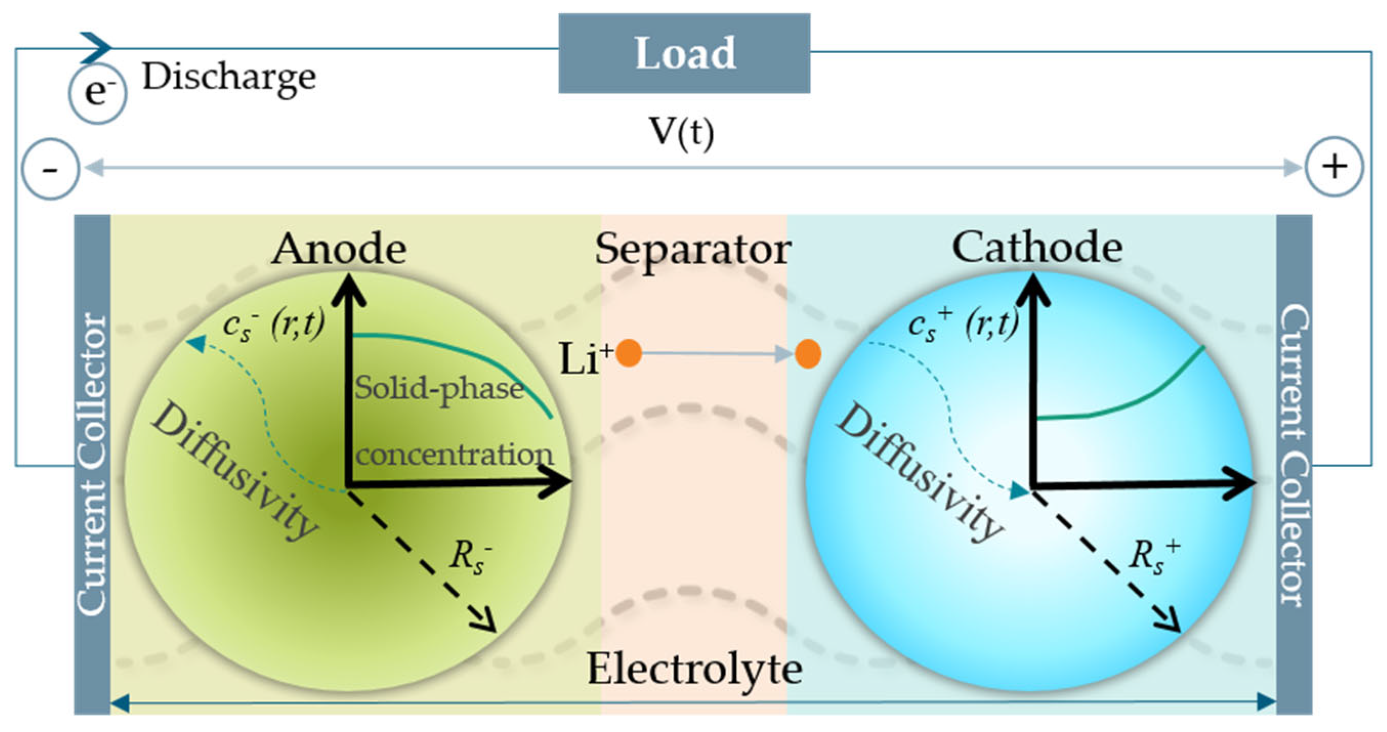
The Doyle–Fuller-Newman (DFN) model is a popular LIB model. A reduced-order form of a DFN model is the SPM, where each electrode is represented as a single spherical porous particle while neglecting electrolyte dynamics [39]. The intercalation process and mass transport are modeled over spherical coordinates. Figure 1 depicts the classic SPM, showcasing the dynamic concentration changes during the discharge process.

The PDEs of a SPM model are in the microscopic spatial domain, i.e., the particle radius. This results in one-dimensional spatial variations, as opposed to the DFN model, which is two-dimensional, as it also includes the variable x, which is the electrode thickness. The reason behind this decoupling is that intercalation reactions typically occur uniformly across both electrodes. During discharge, negative electrode particles delithiate at nearly uniform rates, regardless of their position within the electrode, and a similar behavior is observed during the lithiation of positive electrode particles during charging. This is why a single representative particle in each electrode (i.e., a SPM) can adequately approximate the behavior of the entire electrode [40].

Figure 1. Illustration of a single particle model adapted from [41]. Particle represents the concentration gradient due to solid–phase diffusion. $R_p^{+}$ and $R_p^{-}$ are the particle radius and $c_s^{+}\left(r,t\right)$ and $c_s^{-}\left(r,t\right)$ are the solid–phase Li-ion concentration of the cathode and anode, respectively. $V\left(t\right)$ is the terminal voltage across cell.

Figure 1. Illustration of a single particle model adapted from [41]. Particle represents the concentration gradient due to solid–phase diffusion. $R_p^{+}$ and $R_p^{-}$ are the particle radius and $c_s^{+}\left(r,t\right)$ and $c_s^{-}\left(r,t\right)$ are the solid–phase Li-ion concentration of the cathode and anode, respectively. $V\left(t\right)$ is the terminal voltage across cell.

Li-ions move from the negative electrode to the positive electrode during discharging and in the opposite direction during charging. Lithium concentration in the solid phase, i.e., concentration of Li-ions in the active materials, follows the laws of diffusion [42]. The electrochemical reaction that takes place in the electrode materials of LIBs involves two kinetic behaviors during charging and discharging: the insertion and extraction of Li-ions and the transfer of electrons/charges that occur during the oxidation or reduction of the electrode materials [43]. When discharging the battery, Li-ions migrate through the electrolyte from the negative electrode to the positive electrode and generate an electric current, while when charging the battery, Li-ions are released from the positive electrode and return to the negative electrode. The battery cells used in this study are prismatic cells called Lithium-ion Power Cell LP2714897-51Ah-BEV, with a cathode of NMC-622 and a graphite anode. Reaction equations for the discharging process of this cell chemistry are as follows:

Anode: Li_xC₆ → C₆ + xLi⁺ + xe⁻;

(1)

Cathode: Li_1−xNi_0.6Co_0.2Mn_0.2O₂ + xLi⁺ + xe⁻ → LiNi_0.6Co_0.2Mn_0.2O₂;

(2)

Cell: Li_1−xNi_0.6Co_0.2Mn_0.2O₂ + Li_xC₆ → C₆ + LiNi_0.6Co_0.2Mn_0.2O₂;

(3)

As the electrochemical reaction occurs in the electrodes, there is a difference in the distribution of Li-ions on the surface and inside the electrode, creating a concentration gradient that drives Li-ion diffusion [43]. Solid-phase diffusion dynamics are central to an SPM and are represented by Fick’s second law of diffusion. The governing differential equation and its accompanying conditions are explained as follows [44,45,46]:

$$\frac{\partial c_{s,j}\left(r,t\right)}{\partial t}=\frac{D_{s,j}}{r^2} \frac{\partial }{\partial r}\left(r^2\frac{\partial c_{s,j}\left(r,t\right)}{\partial r}\right)$$

(4)

Here, $c_{s,j}$ is the Li-ion concentration in the solid particles, $D_{s,j}$ is the solid-phase diffusion coefficient, $r$ is the radial coordinate, $j=p$ corresponds to the positive electrode, and $j=n$ corresponds to the negative electrode. The boundary conditions at the particle center $\left(r=0\right)$ and particle surface $(r=R_j$) are:

$${\left.\frac{\partial c_{s,j}\left(r,t\right)}{\partial r}\right|}_{r=0}=0 at r=0 and t\ge 0$$

(5)

$${\left.\frac{\partial c_{s,j}\left(r,t\right)}{\partial r}\right|}_{r=R_j}=\pm \frac{I\left(t\right)}{A{L}_{j}F{D}_{s,j}{a}_j} at r=R_j and t\ge 0$$

(6)

Here,$I\left(t\right)$ is the charge/discharge current, $A$ is the battery sheet area, $L_j$ is the thickness of the positive and negative electrode, $a_j$ is the specific interfacial area: $a_j=3{\epsilon }_j/R_j$, where ${\epsilon }_j$ is the solid phase volume fraction of each electrode and $F$ is Faraday’s number. The initial condition is given by:

$$c_{s,j}=c_0 at t=0 and 0\le r\le R_j atfullychargedstate$$

(7)

Equations (4)–(7) are now simplified via the dimensionless variables introduced in [45].

$$C=\frac{c_{s,j}}{c_0}; x=\frac{r}{R_j}; \tau =\frac{D_{s,j}t}{R_j^2}$$

(8)

This results in adaptation of the corresponding governing equation, boundary conditions, and initial condition as given below:

$$\frac{\partial C}{\partial \tau }=\frac{1}{x^2} \frac{\partial }{\partial x}\left(x^2\frac{\partial C}{\partial x}\right)$$

(9)

$$\frac{\partial C}{\partial x}=0 at x=0 and \tau \ge 0$$

(10)

$$\frac{\partial C}{\partial x}=-\delta at x=1 and \tau \ge 0$$

(11)

where δ is the applied dimensionless current density defined as:

$$\delta =\pm \frac{I\left(t\right)R_j}{A{L}_{j}F{D}_{s,j}{a}_j{c}_0}$$

(12)

$$C=1 at \tau =0 and 0\le x\le 1$$

(13)

The SOC of the particles can be calculated by using the electrodes’ minimum and maximum possible solid-phase concentrations [47].

$$SOC=\frac{c_{s,j}-c_{min}}{c_{max}-c_{min}}$$

(14)

Instead of estimating the theoretical values of the maximum and minimum concentrations of the active materials, the stoichiometry value at 0% SOC and at 100% SOC are used for calculating the SOC across the entire discharge time period. Stoichiometry refers to the proportion of the active materials in the electrodes of the battery. At 0% SOC, the battery is fully discharged, and the active materials in the anode ($x_{0\%}$) is in its highest state of oxidation (i.e., it has given up electrons). In contrast, at 100% SOC, the battery is fully charged, and the active materials in anode ($x_{100\%}$) is in its lowest state of oxidation (i.e., it has accepted electrons).

$$SOC\left(t\right)=\frac{\frac{c_{s,j}}{c_{s,max}}-x_{0\%}}{x_{100\%}-x_{0\%}}$$

(15)

The concentration of solid-phase Li-ions in the anode of a LIB cell is directly related to the cell capacity. A high concentration of Li-ions in the anode results in a higher battery capacity, while a lower concentration results in a lower capacity. Overall, the concentration of solid-phase Li-ions in the anode is a critical factor in determining the capacity and performance of LIBs [38].

In the context of model-based estimation, SOH refers to the actual performance of a battery, normalized by the performance when the battery was new. In fact, any battery parameter that changes with usage can be used as an indicator for SOH [5]. Common metrics of interest for a battery management system (BMS) are capacity, impedance and internal resistance. In this paper, capacity-based SOH is studied.

The capacity across the time period can be derived using Equation (15). $C_{nominal}$ is the nominal capacity provided by the manufacturer, and $C_{max}$ is the capacity at the beginning of the life of the cell.

$$C\left(t\right)=SOC\left(t\right)\times C_{nominal}$$

(16)

$$SOH=\frac{max\left(C\left(t\right)\right)}{C_{max}} at 100\% SOC$$

(17)

Hence by describing the diffusion problem and presenting the set of equations above, we have established a foundation for estimating the SOC and SOH of battery cells.

4. Architecture and Methodology

In this section, we will first provide a concise overview of the PINN algorithm proposed by Raissi et al. [48,49] for solving non-linear PDEs. For a more detailed understanding of the PINNs algorithm, we recommend interested readers refer to [23,50]. However, for instructional purposes, we explain the algorithm by applying it to the problem explained in the previous section (Section 3) accompanied by Neumann boundary conditions. $C\left(x,\tau \right)$ is the unknown solution derived in Equation (9).

$$C_{\tau }=\frac{2}{x}{C}_x+C_{xx} ; x\in \left[0,1\right],\mathsf{\tau }\in \left[0,\frac{D_{s,j}t}{R_j^2}\right]$$

(18)

(see Equation (8))

$$C_x\left(0,\tau \right)=0$$

(19)

$$C_x\left(1,\tau \right)=\pm \delta$$

(20)

Here, the sign of $\delta$ depends on charge/discharge cycles in the Equation (12).

$$C\left(x,0\right)=1$$

(21)

Automatic differentiation is employed to calculate the derivatives of the NN $C\left(x,\tau \right)$ with respect to the normalized time τ and space x, applying the chain rule for differentiating compositions of functions [51]. In order to compute the derivatives required in the above equations, modern deep learning frameworks such as Pytorch and Tensorflow [52] are used. They are widely used and well-documented open-source frameworks for automatic differentiation and deep learning computations.

We approximate the unknown solution $C\left(x,\tau \right)$ to the Fick’s diffusion equation by a deep NN. Consequently, the corresponding function for PINN takes the following form, $f\left(x,\tau \right)$:

$$f≔ C_{\tau }-\frac{2}{x}{C}_x+C_{xx} ;$$

(22)

The shared parameters between the NNs, $C\left(x,\tau \right)$, and $f\left(x,\tau \right)$ are learned by minimizing the mean squared errors loss function.

$$MSE=MS{E}_0+MS{E}_{NBC}+MS{E}_f$$

(23)

Here,

$$MS{E}_0=\frac{1}{N_0}{\displaystyle \sum }_{i=0}^{N_0}{\left|C\left(x_0^i,0\right)-1\right|}^2$$

(24)

$$MS{E}_{NBC}=\frac{1}{N_b}{\displaystyle \sum }_{i=0}^{N_b}\left({\left|C_x\left(0,{\tau }_b^i\right)-0\right|}^2+{\left|C_x\left(1,{\tau }_b^i\right) \pm \delta \right|}^2\right)$$

(25)

$$MS{E}_f=\frac{1}{N_f}{\displaystyle \sum }_{i=0}^{N_f}{\left|f\left(x_f^i,{\tau }_f^i\right)\right|}^2$$

(26)

Here, ${\left\{x_0^i\right\}}_{i=0}^{N_0}$ denotes the initial data generated in this example by the initial condition. ${\left\{{\tau }_b^i\right\}}_{i=0}^{N_b}$ corresponds to the collocation points on the boundary, and ${\left\{x_f^i,{\tau }_f^i\right\}}_{i=0}^{N_f}$ represents the collocation points on the residual network $f\left(x,\tau \right)$. Collocation points are specific points at which the loss functions are minimized in order to enforce the governing equations. 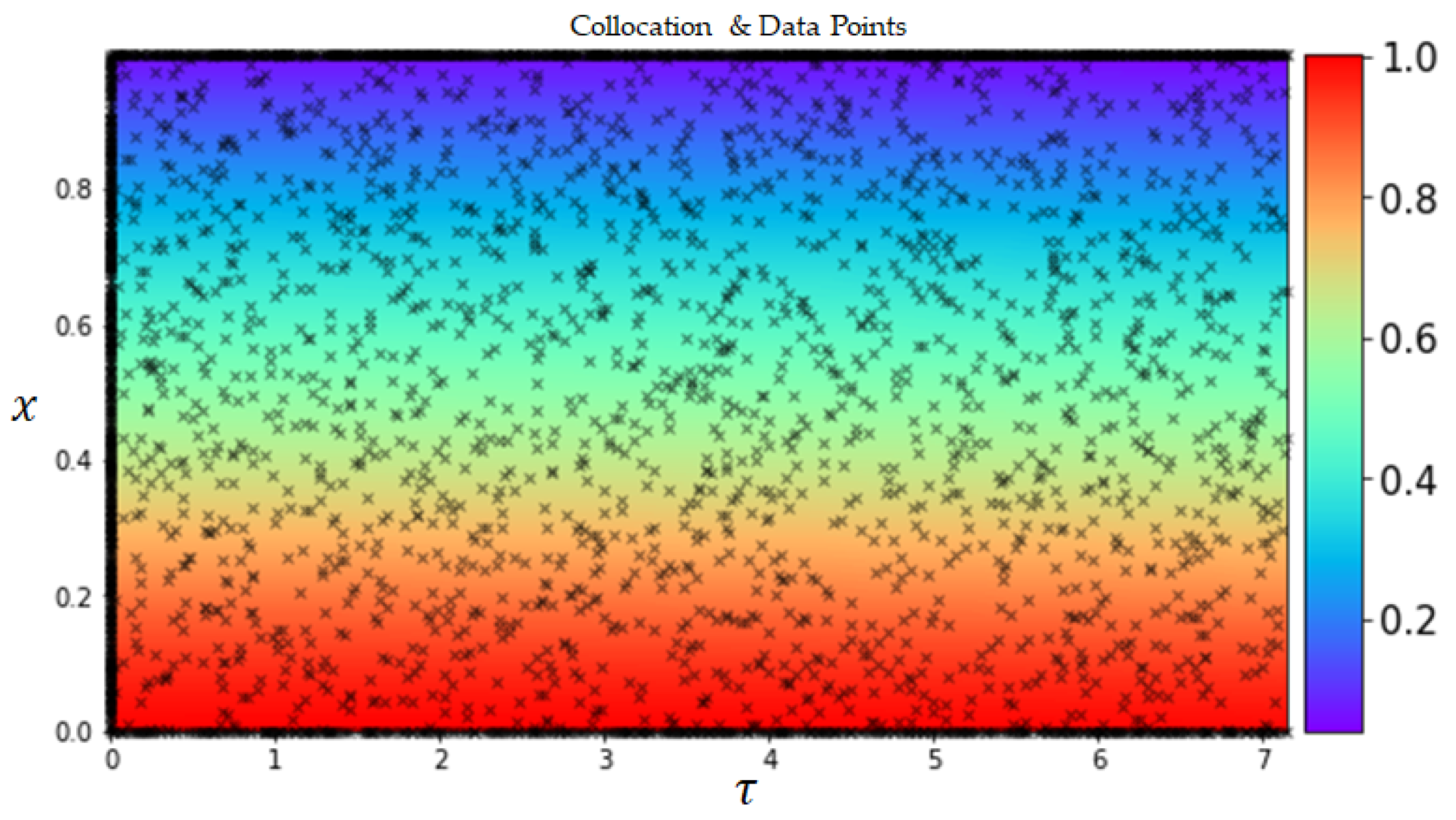They can be interpreted similarly to nodes in finite element methods [30]. Collocation points should not be confused with data points. Data points refer to the input-output pairs of data that are obtained from experiments or simulations.

Figure 2 shows the collocation points used in this study across the spatio-temporal domain for solving Fick’s diffusion equation. In such a continuous time NN, a significant number of collocation points $N_f$ are required to enforce physics-informed constraints. Although this poses no significant issues for problems in one or two spatial dimensions, it may introduce a bottleneck in higher-dimensional problems as the total number of collocation points needed to globally enforce a physics-informed constraint (i.e., in our case, a PDE) will increase exponentially [49].

Consequently, the loss on the initial condition is represented by $MS{E}_0$, $MS{E}_{NBC}$ enforces the Neumann boundary conditions, and $MS{E}_f$ penalizes any deviation of Fick’s diffusion equation from satisfaction on the collocation points. This example effectively encompasses all the key aspects of the PINN algorithm and can be extended to different PDEs requiring individual treatment of boundary conditions.

Next, this section will provide further details of our utilized architecture and the approach for interacting with inputs and outputs. Our methodology draws inspiration from the contributions of [53,54].

4.1. Experimental Data

This section describes the experiments conducted for the study. As mentioned before, the battery cells used are the prismatic cells called Lithium-ion Power Cell LP2714897-51Ah-BEV, with a cathode of NMC-622 and a graphite anode. Cell specifications are summarized in

Table 1. Cell specifications and input parameters for the model.

Symbol	Value	Unit	Denotation
Cnominal	51	Ah	Nominal Cell Capacity
A	1.843	m2	Electrode surface area
x0%	0.028		Stoichiometry anode (SOC = 0%)
x100%	0.794		Stoichiometry anode (SOC = 100%)
y0%	0.914		Stoichiometry cathode (SOC = 0%)
y100%	0.344		Stoichiometry cathode (SOC = 100%)
L+	55.5 × 10−6	m	Cathode thickness
L−	67.3 × 10−6	m	Anode thickness
R+	3.28 × 10−6	m	Cathode particle radius
R−	6.72 × 10−6	m	Anode particle radius
ε+	0.755		Active material volume fraction cathode
ε−	0.7		Active material volume fraction anode
$c_{s,max}^i$1	36,129.55	mol/m3	Maximum theoretical solid-phase concentration of Li+ ions in the electrodes
I	−17 to 17	A	Charge and discharge current input
t	$f\left(I\right)$	s	Time corresponding to the input current

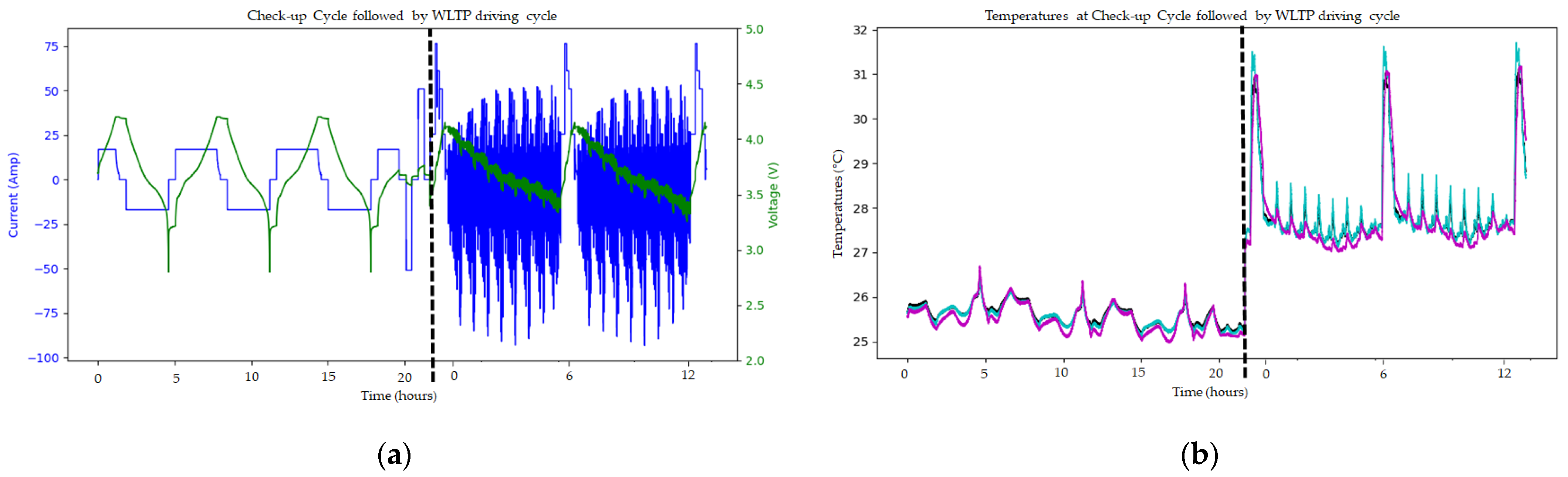
¹ i = p for cathode and i = n for anode.

. The cell dimensions and kinetic parameters of the cell are obtained from a trusted third-party source. However, the exact approach used to determine the internal cell parameters cannot be disclosed due to confidentiality restrictions. Three cells were subjected to consistent environmental conditions within climate chambers with designated ambient temperatures (Cell 3–25 °C, Cell 5–45 °C, and Cell 7–5 °C).

The experimental test procedure for each cell involved an initial check-up at the beginning of life, followed by cycling through 100 worldwide harmonized light vehicle test procedures (WLTP) at a specific temperature, followed by check-up test cycles after every 100 WLTP cycles, and then a final check-up at end-of-life. The climate chamber was brought to an ambient temperature of 25 °C, and only once the cell reached a thermal steady state, the check-up procedure was performed. The check-up procedure involved a differential voltage analysis, a pulse test, electrochemical impedance spectroscopy, and a capacity check. Only the capacity check-ups cycles are used in this study as an input to the PINN. However, to give an idea of the cycling tests performed during the experiments, Figure 3 represents both the check-up cycle followed by the driving cycle of cell 3.

4.2. Data Preparation

This subsection sheds light on data preparation for training and validation. The difference in the magnitude of input parameters is problematic when computing using ML algorithms. The presence of larger data points in non-normalized data sets can lead to instability in the NNs, as the relatively large inputs can propagate down the network layers and cause cascading effects. To prevent this issue, the input data for PINN should be normalized. This involves converting the original values to new values and bringing most parameters into the same range. This allows the gradient descent optimization algorithm to converge faster and obtain a mean close to zero since the learning speed is proportional to the magnitude of the inputs. For our network, the equation (Equations (9)–(13)) resulting from the dimensionless parameters are used to setup the network. The input parameters required for PINN are also summarized in Table 1.

4.3. Architecture

In this work, the output variable (i.e., concentration) is approximated via a fully connected FNN. The network has three types of layers. The first layer is the input layer. Next, there are hidden layers in between. Finally, there is the output layer. Each layer can contain several neurons, and there is no connection between neurons inside a layer. Moreover, each layer is connected to the next layer to pass information from the input layer to the output layer. A neuron transforms an input x into an output as follows:

$$z\left(x\right)=\alpha \left(Wx+b\right)$$

(27)

where $\alpha$ is a chosen nonlinear parameter called activation function, $W$ is the weight matrix, and $b$ is a correction term called bias. Each input $x$ is given a weight $W$. The weights determine the degree of influence the neuron’s inputs have on calculating subsequent activation. The purpose of an activation function is to add nonlinearity to the NN, and a proper choice of the activation function is problem dependent. They should be differentiable so that the parameters of the network are learned in backpropagation.

The backpropagation algorithm works by computing the gradient of the loss function with respect to each weight and bias in the network, starting from the output layer and working backward through the layers. The gradients are computed using the chain rule. Once the gradients are computed, they are used to update the weights and biases using a technique called gradient descent. In gradient descent, the weights and biases are adjusted in the direction that reduces the loss function the most by multiplying the gradient by a learning rate and subtracting it from the current values of the weights and biases. This process is repeated iteratively until the loss function reaches a minimum or a convergence criterion is met. Various optimization techniques can be employed to improve the effectiveness of the weight and bias updates in the NN. Moreover, the hyper-parameters affect the network’s performance, such as activation function, learning rate, number of epochs, batch size, hidden layers, and neurons in each layer. The effect of the choice of hyper-parameters on the network is studied in [30]. The optimization methods and hyper-parameters selected in this paper are elaborated in Section 4.4.

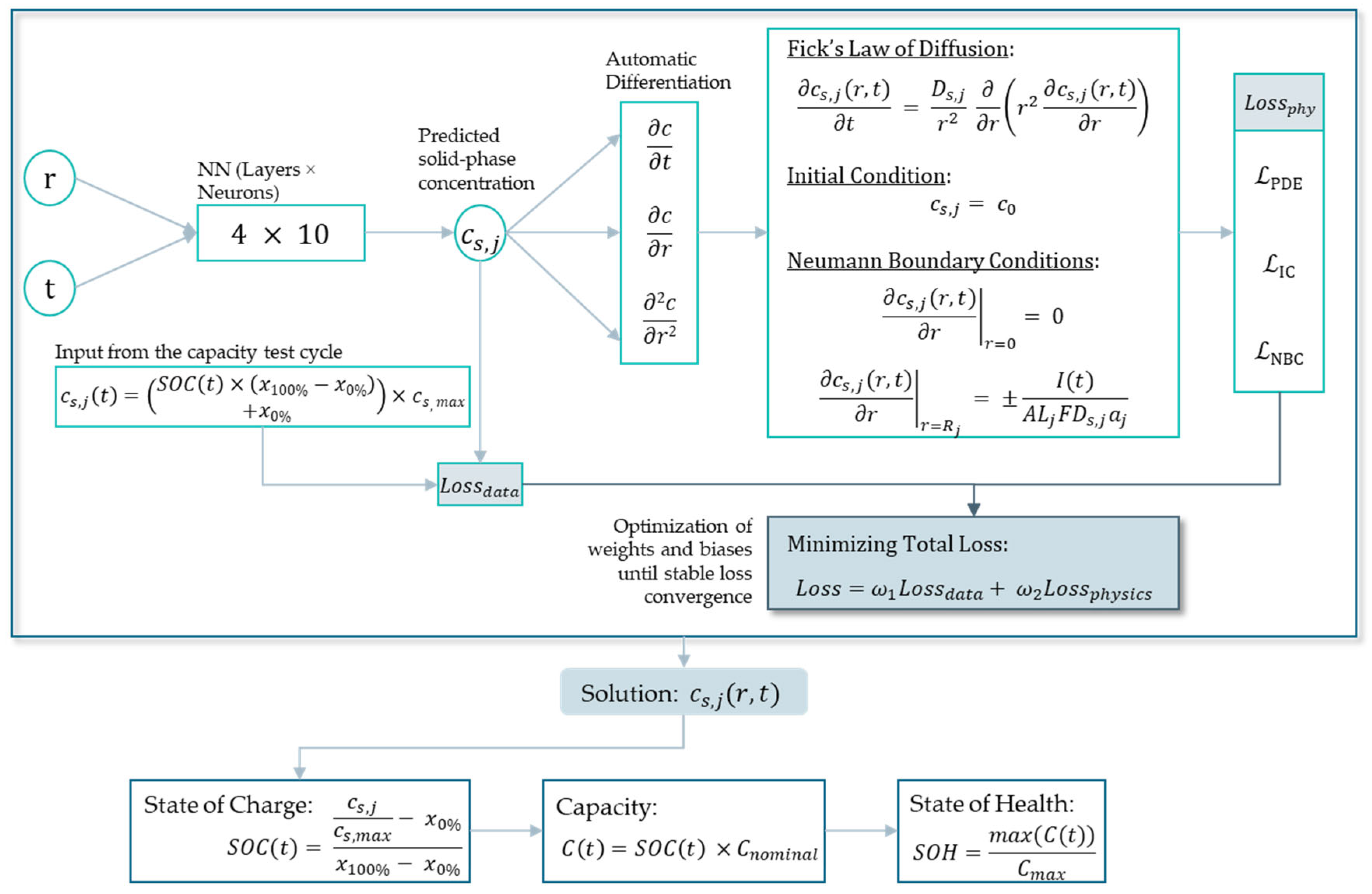
The PINN formulation for the diffusion problem of LIBs can be depicted in Figure 4. The network is based on Equations (4)–(26). The inputs for the PINN model are a spatial vector, particle radius (r) across a grid size of 100, and a temporal vector, time (t). The two inputs are then used to construct a mesh, which is a set of points in space and time used to approximate the solution to a given PDE. Along with this, the network also gets the concentration value from the measurement data. This is derived using Equation (15). The rate of change in SOC across the time series input as well as the stoichiometry ratios at 0% and 100% SOC need to be known for training purposes. Additionally, the current subjected to the cell is also given as a time series input used for calculating the molar flux in Equation (12). The trainable set of parameters are {W,b}. Solid-phase concentration of lithium is the output of the network and is a function of the trainable parameters. Training is performed by minimizing the total loss.

The solution to the diffusion problem using PINN is acquired by ensuring that the NN satisfies the diffusion equation at every point in the domain. This is done by adding a term to the loss function that penalizes any deviation from the diffusion equation. Specifically, the loss function is given by:

$$Loss={\omega }_{1}Los{s}_{data}+{\omega }_{2}Los{s}_{physics}$$

(28)

where $Los{s}_{data}$ is the data-fitting term that measures the difference between the predicted and the actual concentration, $Los{s}_{physics}$ is the physics-informed term that enforces the diffusion equation, and $\omega$ is the weighting factor that balances the two terms. The physics-informed term is formulated by taking the gradients of the predicted concentration with respect to time and space and plugging them into the diffusion equation. The output of the PINN is the solid-phase concentration. Using this solution, the Equations (15)–(18) are executed, which yield the time-dependent SOC and SOH of the battery cell.

The above presented architecture differs from previous architectures of PINN because, here, the training is done on the basis of Neumann boundary conditions instead of the previously used Dirichlet boundary conditions. This is achieved by creating a separate serial input (current and time) for the boundary condition. The Neumann boundary condition is then solved in a separate FNN trained only on the basis of the calculated value of the maximum boundary condition.

4.4. Training, Validation and Testing Data

Input data for the PINN are split among training, validation, and testing data. Radial and time vectors are merged into a mesh {X,T} to represent each location at each time point of the particle. To solve the PDE, a predefined number of collocation points over the entire mesh {X,T} is used. The data are split into 80% training and 20% validation data. Different ratios, such as 70:30 and 90:10, were also tested, but a trade-off is reached with respect to the training time and performance on the test set. The entire mesh is then given as input to the PINN for the testing process. By monitoring the performance on the validation split during training, we define when to stop the training in order to avoid overfitting. Additionally, a termination tolerance of 1 × 10⁻⁵ is set to ensure that the training stops when the loss function improvement falls below the given threshold.

The activation function utilized in this work is Hyperbolic-Tangent (tanh) function. Minimization of the loss function is completed by the Adam optimizer [55]. The initial learning rate is set to 1 × 10⁻³ and the final learning rate to 1/100 of the initial learning rate. ‘ExponentialDecay’ learning rate scheduler is then used to gradually reduce the learning rate over time. In order to prevent overfitting, the ‘EarlyStopping’ callback function is used to monitor the training process. Adaptive weights are used to dynamically adjust the weights assigned to each loss term in the total loss function during training. This is implemented using the GradNorm method [56]. This is done in order to address the issue of gradient pathology, where loss terms with higher derivatives tend to dominate the total gradient vector and negatively affect the accuracy of the solution.

5. Results and Discussion

Due to space constraints, we have included only the plots of the anode in this section. However, we would like to note that, similar to the anode behavior, the PINN used for deriving the concentration change across the cathode also satisfied the physical constraints.

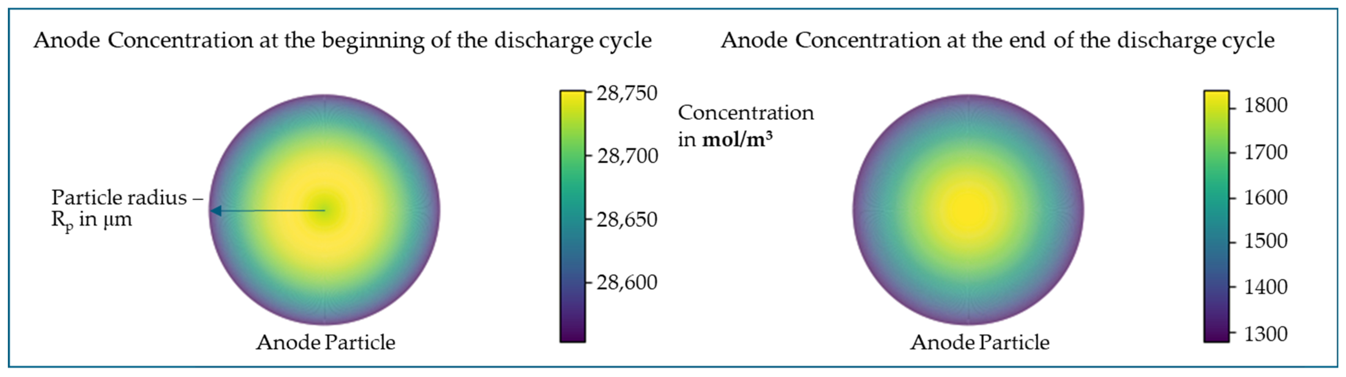
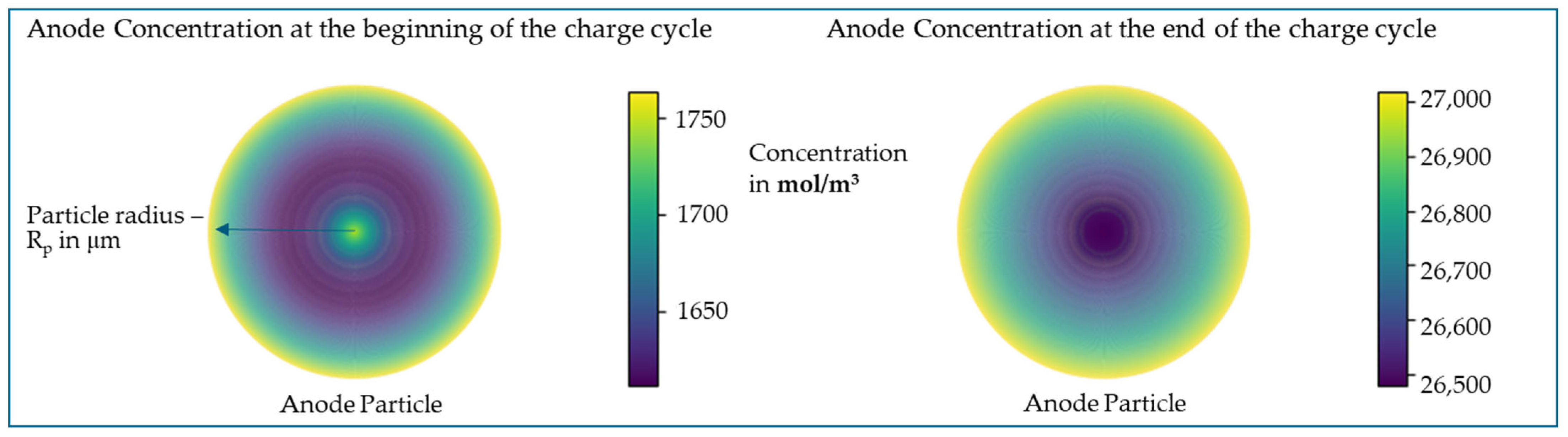
The following set of results describes how the Li-ion concentration changes inside a particle driven by a concentration gradient based on Fick’s law of diffusion. Figure 5 represents the anode particle at the beginning and end of a CC discharge cycle, where the SOC changes from 100% to 0%. Similarly, Figure 6 shows the anode particle at the beginning and end of a CCCV charge cycle, where the SOC changes from 0% to 100%.

During discharge, Li-ions leave the anode and diffuse through the electrolyte and separator to the cathode. As a result, the Li-ion concentration of the anode decreases over time and radius. In reality, at a SOC of 100%, there is still a significant amount of Li-ions intercalated in the cathode, which is why the anode does not reach the maximum theoretical concentration. The rate of change in anode concentration at the center of the particle, i.e., at r = 0, is almost constant, as per the minimum boundary condition (Equation (5)). At the particle surface, i.e., at r = R_p, the rate of change in Li-ion concentration depends on the molar flux density, as per the maximum boundary condition (Equation (6)).

When training the PINN, the loss function consists of multiple components, as explained in Equation (23). The loss function measures how well the NN is satisfying the governing PDE of the problem. A decreasing trend of the losses indicates that the PINN is learning the governing physics, and boundary conditions and progressing toward a better approximation of the solution. Minimization of the loss function is affected by the choice of hyper-parameters such as learning rate, number of epochs, type of optimizer, and number of input samples. Therefore, selecting appropriate hyperparameters is crucial for optimizing the loss function. Figure 7 shows that around 500 epochs are needed to converge the optimization process. Measures taken to avoid the overfitting of data were already elaborated in Section 4.4.

In order to verify the diffusion behavior across the anode, an approach described in the reference paper [47] is used. Here, a novel analytical approach to determind the Li-concentration within the electrode particles is derived and coupled to the ECM and implemented in MATLAB. The output of the analytics model is mainly used to verify the linear and quadratic behavior of the concentration curves, given the same set of input parameters.

5.1. State of Charge Estimation

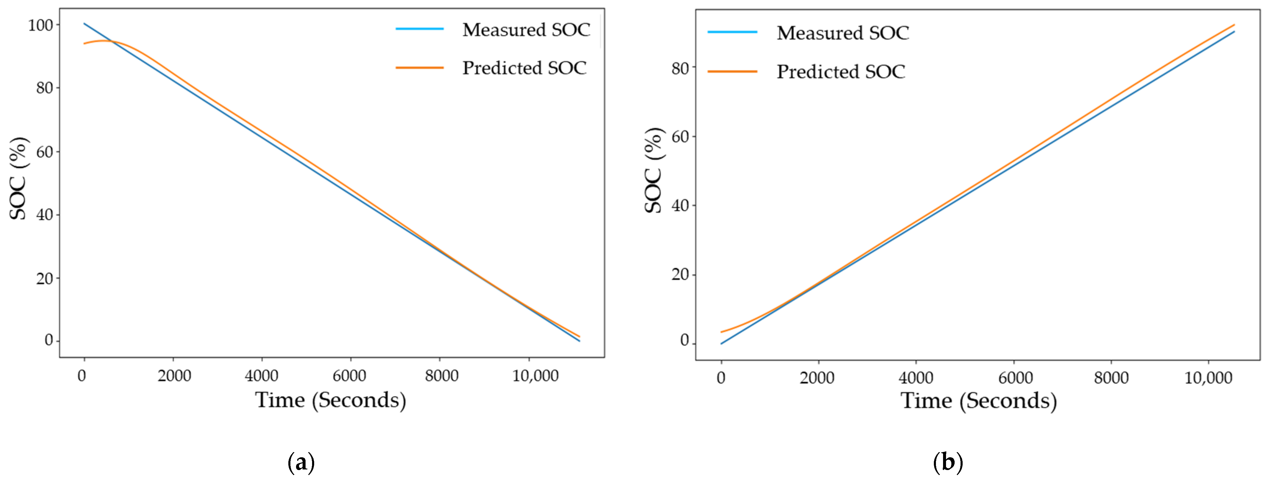
Figure 8 shows the output plots of the estimated SOC compared to the measured SOC during a complete charge and complete discharge cycle. For every new check-up cycle, the PINN is trained for multiple cycles, and the change in SOC with respect to time is estimated using Equation (15). The quadratic behavior of the concentration due to the PDE in Equation (9) is responsible for the nonlinear behavior of the PINN SOC estimation. Across the capacity check-up cycles, it is noted that the root mean square error (RMSE) for SOC estimation lies between 0.014% and 0.2%.

5.2. State of Health Estimation

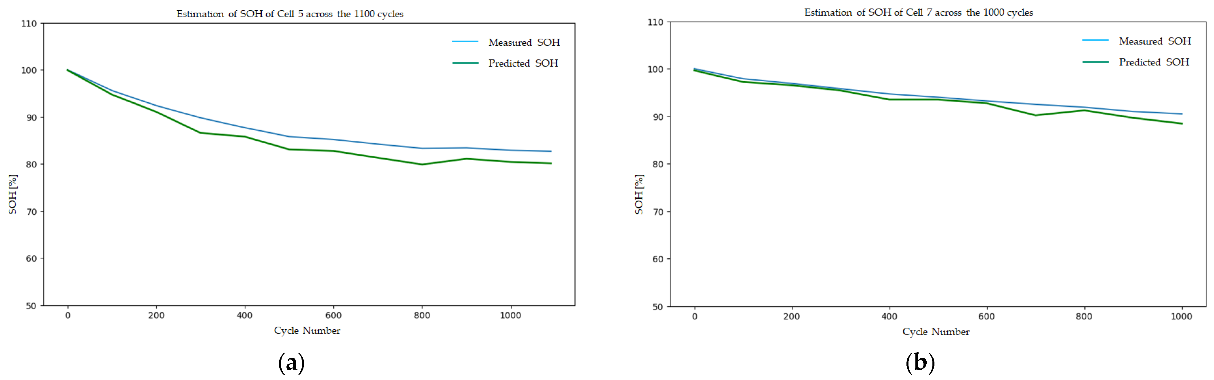
The PINN is executed iteratively across all check-up capacity test cycles to determine the SOH of the cells. At the beginning of each new check-up cycle, the concentration value must be reset to the output value of the previous cycle. SOH is calculated by determining the maximum available capacity with respect to the concentration of Li⁺ in the anode, as per Equations (16) and (17). Figure 9 shows the measured and predicted SOH plots for cell number 5 and cell number 7. The RMSE of SOH estimation for cell 5 is 2.381% and for cell 7 is 1.176%. The change in temperature for cell cycling does not majorly affect the PINN performance for SOH estimation.

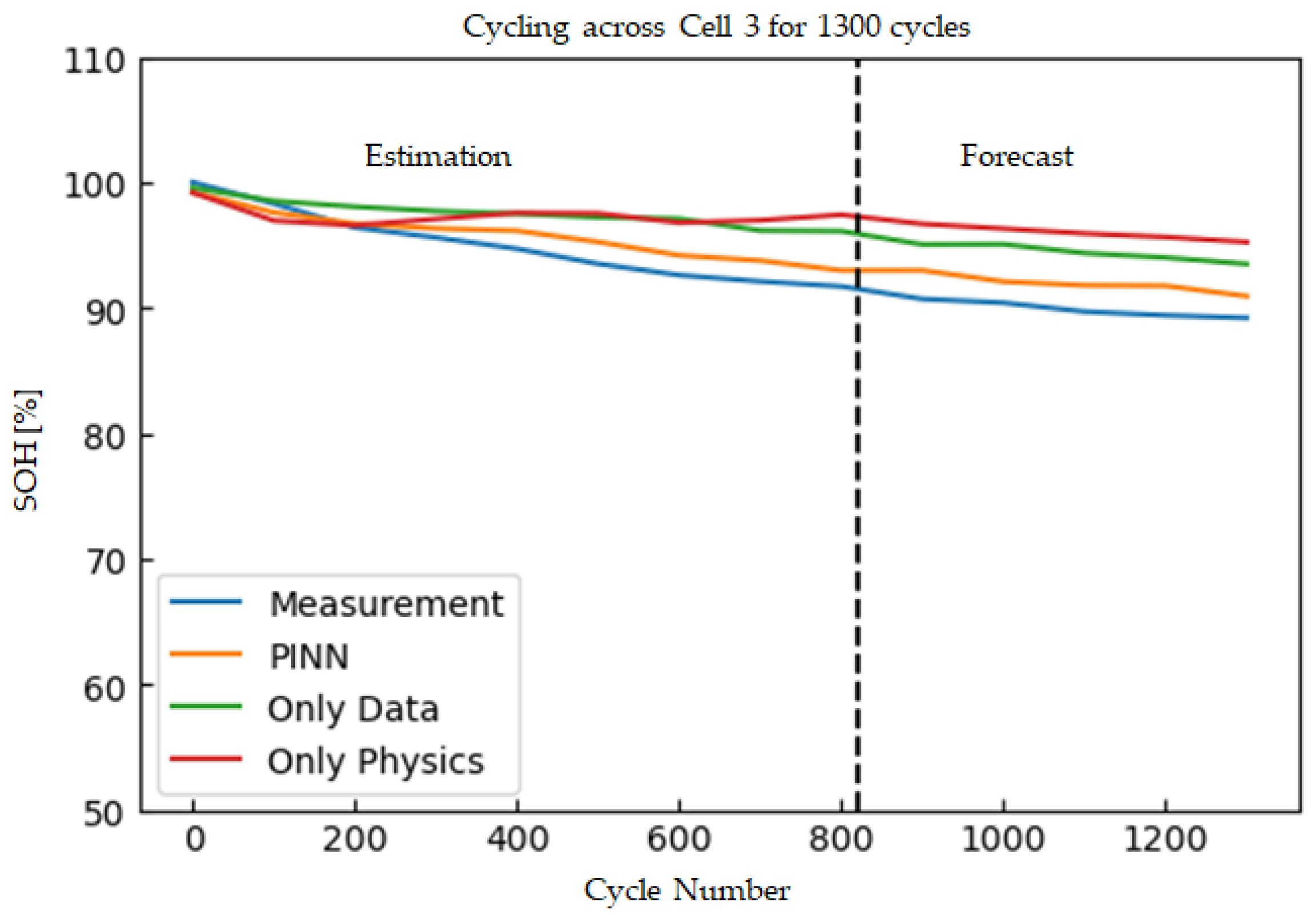
In order to investigate the differences between training the NN solely on data or solely on the underlying physics, as opposed to training on a combination of both data and physics, we conducted a specialized training procedure on cell number 3.

The procedure is that during training, the different components of the loss function are selectively included in or excluded from the loss function (see Equation (28)). If the network is to be trained solely on the basis of physical constraints, the component of the loss function that represents the data is excluded (${\omega }_1=0$ and ${\omega }_2=1$), thereby resulting in a curve that represents ‘Only Physics’ (see Figure 10). Conversely, if the network is to be trained solely on the basis of data, the component of the loss function that represents the physical constraints is omitted (${\omega }_1=1$ and ${\omega }_2=0$), thereby resulting in a curve that represents ‘Only Data’. If both components of the loss function have been included (${\omega }_1=1$ and ${\omega }_2=1$), the resulting curve represents ‘PINN’. This approach allowed us to assess the relative impact of the available data and governing equations on the training process and to determine the extent to which each factor contributes to the overall performance of the network.

Additionally, to facilitate testing and evaluation of the model, the input data are partitioned into two sets such that the first eight check-up cycles are reserved for training, while the remaining five check-up cycles are used for testing. Hence, the first set is utilized to estimate the SOH, while the second set is utilized to forecast the SOH.

The results of this approach are shown in Figure 10, which shows the convergence behavior of the network during training for different combinations of data and physics-based inputs. To quantify the accuracy of the predictions, we computed the RMSE for each of the three types of curves, as reported in

Table 2. RMSE of SOH prediction.

	PINN	Only Data	Only Physics
RMSE	1.32%	3.48%	3.94%

. The findings suggest that the combination of data and physical constraints yields improved prediction accuracy compared to using the other two approaches in isolation. Specifically, the RMSE values associated with the combined approach are lower than those associated with the purely data-driven or physics-based approaches. This suggests that by leveraging both data and physics-based constraints, we are able to achieve a more accurate model.

By systematically varying the proportion of data and physics-based inputs used to train the network, we could quantify each factor’s relative influence on the resulting performance. By allowing the model developer to adjust the weights of the terms based on their level of confidence in the available data and underlying physical principles, we get a model with high flexibility to incorporate both data-driven and physics-based information. These findings provide valuable insights into the underlying mechanisms that drive the success of PINN and have important implications for the development of more accurate and robust hybrid battery models with the potential to generalize to new and unseen scenarios.

The results of this study demonstrate the potential of using PINN to accurately estimate SOC and SOH of LIBs operating at three different temperature ranges, even with limited training data and relatively low computational complexity and training time. This approach offers advantages in scenarios where the amount of available data changes adaptively, such as at the beginning of a battery’s life when experimental data acquisition is extensive, but during operation after many usage cycles, experimental data is no longer valid or possible to acquire. Thus, for such scenarios, PINN is well-suited for application in a battery digital twin because automatic parameter updates are one of the main requirements of battery DT implementation [57]. Further work will focus on extending the PINN approach and integrating it into a battery digital twin.

While the accuracy of this approach cannot be claimed to always outperform existing state estimation approaches in all operational scenarios, this study provides a promising starting point for the systematic integration of PDEs of P2D models into NNs. Moreover, a limitation of this study is the assumption of a constant diffusion coefficient due to isothermal conditions, whereas in real-world scenarios, the diffusion coefficient changes with battery aging and affects the concentration behavior at the electrodes.

Further exploration is needed to overcome challenges associated with developing hybrid battery models using PINN. Future research can also investigate different network architectures and their effects on integration with PDEs. Additionally, the proposed PINN can be expanded to include additional physical constraints, such as the heat generation equation or the Butler–Volmer equation. Finding the optimal balance between the flexibility of machine learning and the accuracy of physics will be a crucial area of future investigation.

6. Conclusions

In conclusion, this paper proposes a novel approach for hybrid battery modeling using PINN and demonstrates its effectiveness in estimating the SOC and SOH of LIB cells. By incorporating the laws of physics into the training process, the proposed approach could produce adequate predictions even for unseen situations. The RMSE of SOH prediction using the developed PINN was 1.32%, 2.381%, and 1.176% for cell 3, cell 5, and cell 7, respectively. Additionally, the SOC prediction exhibited a variance of 0.014% to 0.2%.

The findings of this study reveal the capability of PINN to enable flexibility in battery modeling. Specifically, the flexibility arises from the ability to select a data-driven model when sufficient training data are available. However, in cases where the amount of training data is insufficient, PINNs can still enhance the accuracy of the model by incorporating prior knowledge of the underlying physics. Therefore, this is potentially a valuable tool for BMS algorithms.

Future work includes applying this approach to other battery chemistries and optimizing the PINN architecture for better performance. Looking forward, the proposed hybrid model will be integrated with the digital twin of a battery cell and battery module to reflect the actual aging and degradation of the physical battery. Using PINN for battery digital twin implementation to predict the SOH, we can learn the physical dynamics of a battery in terms of differential equations and automatically update the model parameters based on their solutions. This is a novel approach for implementing the model component of a battery digital twin that can learn the physics of battery aging and reflect it in the lifetime predictions made by the model.

This study contributes to bridging the gap between traditional physics-based modeling and modern data-driven ML techniques, as shown by the performance of the proposed approach compared to a purely physics-based model and a classical black-box NN.