Article

Flow Modeling of a Non-Newtonian Viscous Fluid in Elastic-Wall Microchannels

by
A. Rubio Martínez
1,2,
A. E. Chávez Castellanos
2,
N. A. Noguez Méndez
3,
F. Aragón Rivera
4,*,
M. Pliego Díaz
1,
L. Di G. Sigalotti
5,* and
C. A. Vargas
5
1
Tecnológico Nacional de México, Campus Querétaro, Av. Tecnológico s/n esq. Mariano Escobedo, Centro Histórico, Querétaro 7600, Mexico
2
Facultad de Química, Universidad Nacional Autónoma de México, Ciudad Universitaria, Ciudad de México 04510, Mexico
3
Departamento de Sistemas Biológicos, Universidad Autónoma Metropolitana, Unidad Xochimilco, Calzada del Hueso No. 1100, Villa Quietud, Ciudad de México 04960, Mexico
4
Departamento de Energía, Universidad Autónoma Metropolitana, Unidad Azcapotzalco (UAM-A), Av. San Pablo 420, Colonia Nueva el Rosario, Alcaldía Azcapotzalco, Ciudad de México 02128, Mexico
5
Departamento de Ciencias Básicas, Universidad Autónoma Metropolitana, Unidad Azcapotzalco (UAM-A), Av. San Pablo 420, Colonia Nueva el Rosario, Alcaldía Azcapotzalco, Ciudad de México 02128, Mexico
*
Authors to whom correspondence should be addressed.
Fluids 2024, 9(3), 77; https://doi.org/10.3390/fluids9030077
Submission received: 3 November 2023 / Revised: 12 February 2024 / Accepted: 1 March 2024 / Published: 19 March 2024
(This article belongs to the Special Issue Pipe Flow: Research and Applications)

Abstract

:
The use of polymer microspheres is becoming increasingly widespread. Along with their most common applications, they are beginning to be used in the synthesis of photonic crystals, microstructure analysis and multiplexed diagnostics for disease control purposes. This paper presents a simple mathematical model that allows us to study the transport mechanisms involved in the deformation of an elastic microchannel under the flow stream of a power-law fluid. In particular, we analyze the momentum transfer to a non-Newtonian fluid (Polydimethylsiloxane, PDMS) due to the deformation of the elastic ceiling of a rectangular microchannel. Hooke’s law is used to represent the stress–deformation relationship of the PDMS channel ceiling. Stop-flow lithography is modeled, and the pressure exerted by the deformed PDMS ceiling on the fluid when the microchannel returns to its original form is taken into account. It is found that the response time of the elastic ceiling deformation increases with the channel width and length and decreases with the channel height independently of the power-law exponent of the injected fluid. However, an increase in the power-law exponent beyond unity causes an increase in the wall-deformation response time and the maximum deformation of the channel height compared to a Newtonian fluid.

1. Introduction

The use of polymer and colloid microparticles is becoming increasingly widespread. In addition to more common applications [1], such as paints, coatings and fractionating columns, emerging applications like optical devices [2], controlled-release drug delivery systems [3,4] and disease diagnosis systems [5] are gaining more and more strength, and while microspheres have been used extensively, non-spherical particles with predetermined anisotropic features are paving the way for the development of new technologies. These technologies include the synthesis of photonic crystals [4] and multiplexed diagnostics microlabs for disease control [6,7]. However, synthesizing these particles is not a simple task. The emulsion polymerization and suspension polymerization processes based on traditional approaches, which are commonly used to synthesize polymer particles, do not ensure a proper control over morphology and anisotropy, which are crucial aspects in the design of non-spherical particles.
Ideally, synthesis processes of such complex particles produce large numbers of monodispersed particles with predetermined anisotropic shapes and properties. In addition, the process allows for the use of functionalizable and biocompatible materials depending on the application requirements. In recent years, various processes focusing on microflows to synthesize particles have been reported in the literature [8]. These methods involve the convergence of two substances of different phases flowing into synthesizing devices, typically T-shaped cylindrical tubes [9,10] or other converging geometrical shapes [11,12]. This setup enables the formation of a large number of monodispersed droplets [9,13] of a precursor monomer for the desired polymer. The next step involves light or thermally induced polymerization into solid droplets [14,15]. However, these methods are significantly limited in terms of the shapes obtained, which typically comprise spheres or sphere-like shapes such as discs [16,17], half-spheres, core-shell spheres [18] and obloids [19,20,21].
New techniques are currently being explored to enhance resolution without compromising the number of synthesized particles. In particular, stop-flow lithography (SFL) is one such technique. This method induces particle formation between two monomer flows, which are brought to a stop within the PDMS microchannel before being flushed out, and this process is repeated cyclically. The efficiency of SFL is closely related to the response of the microflow system to pressure changes, enabling control over the flow frequency in each cycle. One approach employed to control the frequency uses pulsed compressed airflows instead of syringe pumps, thus shortening the response times. Nevertheless, the response time is not instantaneous due to the deformation caused by the airflow pressure on the PDMS elastomer (microchannel) walls. Given the increased use of PDMS in constructing microfluidic channels, it becomes imperative to study the effect of wall deformation on the monomer flow pattern.
The effects of wall deformation in a steady-state rectangular microchannel on the monomer flow profile have been extensively studied [22,23,24,25,26,27,28,29,
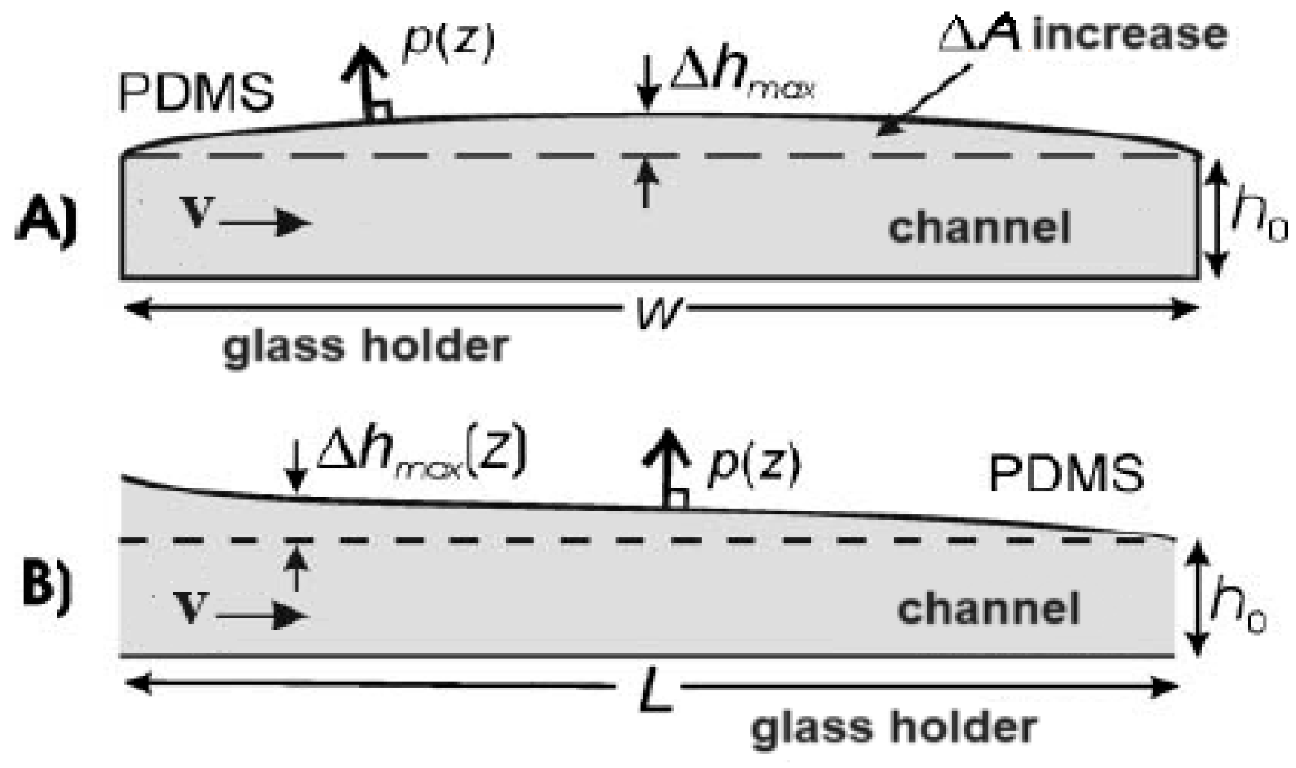
30]. However, the effects on the flow profile of a non-Newtonian monomer due to the dynamic behavior of the walls and the geometry of the PDMS microchannel when subject to external pressure pulses have not been thoroughly addressed. Therefore, it is important to study this behavior in a cyclic process and determine the time required to reach a steady-state condition for the full cycle. In our study, we use a power-law model to describe the effect of the PDMS elastomer walls of a rectangular microchannel on the flow profile of a viscous non-Newtonian fluid in an SFL process (see Figure 1).

Stop-Flow Lithography (SLF) System

Microflow devices usually utilize syringe pumps to inject an incompressible fluid into the device. Inflow through the needle causes flow transitions that may last several minutes in the case of systems on a micrometric scale [27]. Therefore, when a rapid dynamic response is desired, the use of compressed air to inject the fluids into the device is preferable [28]. Even though compressed airflow devices eliminate the pulse pressure gradient transition, there are still finite transitions associated with the PDMS wall deformation.
Three cyclic stages are identified in stop-flow lithography, namely flow interruption, polymerization and fluid flow. During the first stage, thrust pressure on the oligomer stream through the device is stopped, transitioning from a specified entry pressure determined by the compressed air device to atmospheric pressure. The flow takes a finite time to stop, which is a function of the time required for the PDMS channel to retract due to deformation and then regain its non-deformed rectangular cross-section and flush the fluid out of the device. During the second stage, oligomer particles are polymerized during the flow stop, exposing them to UV light by briefly opening (during 0.3 to 1 s) the lamp shutter. During the third stage, the parent particle flows due to the opening of the three-way valve, causing the pressure to change from atmospheric pressure to that of the specified entry pressure. Three specific times can be characterized in this process: the time of flow residence in the channel ( t stop ), i.e., the time when flow is stopped (where t stop > time of wall response t r ), the time required to begin particle polymerization (i.e., the shutter time t shutter ) and the time required to flush the particles out, t f . While t shutter and t f are easily determined, t stop can only be determined after the first estimation of t rp that works as a lower bound for the stop time.

2. Flow of a Viscous Non-Newtonian Fluid through a Microchannel with Elastic Walls

The mathematical model described here is based on a theoretical methodology developed by Dendukuri et al. [24] for Newtonian fluids. Here, a generalization of Dendukuri et al.’s [24] model is developed for power-law fluids.

2.1. Microchannel Geometry

The system under study is a microchannel of height H (before the deformation caused by the circulating flow), length L and width W. The microchannel floor is made of glass lined with a very thin film of PDMS with a Young modulus E = 62 GPa, while the ceiling is made of PDMS that is several millimeters thick with E = 1 MPa. The PDMS characteristics used here were taken from Dendukuri et al. [24]. In addition, this choice represents a good example to determine the characteristic parameters of the system and test new copolymers that are being synthesized in the Polymer Synthesis Laboratory of the Xochimilco Campus of the Autonomous Metropolitan University in Mexico City, which will then be used to replace the PDMS. Thus, the deformation of the channel floor is negligible compared to that of the ceiling. Figure 2 shows a schematic drawing of the cross section of the deformed rectangular channel after a pressure pulse. The flow is from left to right and maximum height deformation in the channel occurs at the entrance and then decreases gradually until it becomes negligible at the exit.

2.2. PDMS Elasticity Modeling

Hooke’s law is used to represent the stress-deformation relationship of the PDMS channel ceiling, which is given by ξ = σ / E , where ξ is the deformation, σ is the stress applied to produce the deformation, and E is the PDMS Young modulus [23]. The stress to which the device is subjected is proportional to the external pressure applied.

2.2.1. Fluid Flow Modeling

To describe the fluid flow under study, we specify the power-law constitutive equation that relates the applied stresses to the resulting deformations. In the present case, the dependent variables are the time-dependent flow velocity v and pressure p. The flow is represented in Cartesian coordinates ( x , y , z ) and the mainstream flow velocity is directed along the x-axis (see Figure 2). In this way, the velocity vector field is
v = ( v x , v y , v z ) = [ v x ( x , z ) , 0 , v z ( x ) ] .
For a steady-state, incompressible fluid, the continuity equation reduces to
v x x + v z z = 0 .
The total stress tensor for this case study will take the following form:
T = p I + σ ̲ ̲ ,
where I is the identity tensor, and σ ̲ ̲ is the shear stress tensor. According to the established velocity field, where movement occurs predominantly along the x-direction and the variations are along the z-direction, the shear stress tensor takes the form
σ ̲ ̲ = 0 0 σ x z 0 0 0 σ z x 0 0 ,
from which Cauchy’s equation in rectangular coordinates reduces to
d σ x z d z = d p d x ,
where h ( x ) = H + Δ h , and σ z x = σ x z . Moreover, the pressure gradient is assumed to be constant along the x-direction, and hence,
σ x z = d p d x z + d p d x h ( x ) 2 .
If σ x z = 0 , then from Equation (6), it follows that z = h ( x ) / 2 .
Substitution of the constitutive equation for a power-law fluid
σ x z = k v x z n
into Equation (5) yields
v x z n = 1 k d p d x z h ( x ) 2 ,
where k and n are the power-law constant and exponent, respectively. Under the boundary condition v x = 0 for z = 0 , integration of the above equation gives the following expression for the mainstream flow velocity
v x ( x , z ) = 1 k d p d x q 1 1 q z h ( x ) 2 q h ( x ) 2 q ,
where the parameter q = ( n + 1 ) / n . This equation describes the flow of a power-law fluid in a rectangular microchannel. If n is an odd number, then Equation (8) describes only real solutions for the flow velocity. In particular, future experiments will be conducted to study the behavior of synthesized copolymers and the power-law fluid model employed here, in addition to approximately describing the behavior of non-Newtonian fluids, allows mathematical prediction to be made more easily and to correlate the experimental data.
Since v x = v x ( x , z ) , it follows from the continuity Equation (2) that
v z ( x ) = h ( x ) q 2 q q 1 k E W q 1 h ( x ) q + 1 q h ( x ) x q + h ( x ) x q
for the z-component of the velocity field. If the above equation is solved for z = h ( x ) , it results in a non-linear differential equation for the instantaneous deformation of the microchannel ceiling h = h ( x , t ) .
A solution to the momentum balance equations for the flow of a power-law fluid in a rectangular channel with an elastic ceiling and rigid floor is here obtained using the lubrication approximations. For this purpose, (i) a system of characteristic variables is specified, (ii) an order-of-magnitude analysis is performed for the balance equations, and (iii) reasonable assumptions based on the physical nature of the phenomenon are made to simplify the equations and allow an analytical mathematical treatment. This allows for an objective description of the system and estimation of analytical results to be compared with previous analytical and/or experimental results.
A PDMS fluid can be considered to be a semi-infinite medium, where the deformations disappear throughout the channel since the PDMS is several millimeters thick, while the channel has a height of only a few micrometers (see Figure 2). Thus, the appropriate length scale to determine the deformation along the z-axis is given by the channel width W, while the deformation of the channel ceiling will be proportional to the ratios of the height increase, Δ h ( x ) , over the channel width, W, and the applied local pressure, p, over the Young modulus, E, [23,26], that is
Ω Δ h ( x ) W p E .
Under the above approximations, the height deformation is then proportional to the local pressure as can be inferred from Equation (10). When the pressure decreases along the length of the channel, the deformation also decreases along the same direction. The maximum deformation is therefore observed at the entrance of the channel and is given by
Δ h max p W E .
Since the height, H, of the microchannel is much smaller than its width, W, i.e., H / W 1 , the deformation of the PDMS-ceiling is negligible along the width. As a consequence, the three-dimensional problem of the fluid flow through the rectangular cross-section reduces to a two-dimensional problem if the height of the deformed channel h ( x , y ) is averaged over the channel width (i.e., along the y-axis), so that the cross-longitudinal section deformation of the device is given by h ( x ) . In addition, if the flow is due to drag ( Re 1 , where Re is the Reynolds number) as is indeed the case here, the equation describing the dynamics of the flow will be given by Equation (6). In passing, it is also important to assume that the PDMS-ceiling curvature is small in relation to the device length.

2.2.2. Coupling between the Elastic Wall and the Flow

When an external pressure is applied to the rectangular cross-section, the device deforms, causing the ceiling to bulge and then return to its original form when the pressure is removed. This in turn gives rise to a compression flow that regulates the flow present in the device. This type of flow is asymmetric in the sense that the flow at the entrance of the channel is greater than that at the exit, with the flow being sustained until the excess fluid is flushed from the device. This process is associated with a characteristic time, which is a function of the properties of the elastic-wall material (PDMS in this case), the fluid (oligomer), the channel geometry and the pressure applied. In this elastohydrodynamic problem, the deformed PDMS ceiling exerts a pressure on the fluid when the microchannel returns to its original form [27,29].
For small deformations, the pressure exerted on the fluid throughout the channel can be considered to be proportional to the deformation of the elastic PDMS wall, according to Equation (11). The length scale for the stress is the channel width, W, so that the pressure along the channel is given by
p ( x ) = E Δ h ( x ) W = E h ( x ) H W ,
where, as it was previously mentioned, H is the height of the non-deformed channel. Thus, its variation as a function of x will be
p x = E W h x .
The scale analysis reveals important features of the problem. Since the channel deformation is small compared to the height of the channel, then
H p W E .
Also h H , which means that the deformation can be approximated as Δ h P W / E , the length as x L and the time as t t r (where t r is the response time of the elastic wall of the device and must be determined for each of the partial derivatives of the equation describing the deformation velocity for the microchannel elastic ceiling). Hence, the velocity along the z-axis becomes
v z = h t p W E t r ,
while
h ( x ) x q p W E L q ,
and
h q h x q H p W E L q .
Substitution of Equations (15)–(17) into Equation (9) gives the following relation
p W E t r H q 2 q q E K W q 1 1 q + 1 H p W E L q + p W E L q .
Furthermore, since H p W / E , the second term inside the brackets in the above equation can be neglected, so that
t r 2 q q ( q + 1 ) L q H q + 1 K W E q + 1 .
From this equation, two important conclusions can be drawn. First, the response time is independent of the pressure, and second, it is inversely proportional to the Young modulus ( E ) as long as the applied pressure does not cause a deformation of the channel height.
In order to calculate the height deformation along the channel, two dimensionless variables are defined, namely Θ = h ( x ) / H and ϵ = x / L , where h ( x ) is the variable height of the channel induced by the pressure gradient, H is the height of the non-deformed channel, x denotes any position along the channel, and L is the channel length. Thus, Equation (19) is recast in the form
h ( x ) Θ q + 1 2 q q ( q + 1 ) 1 t r x ϵ q K W E q 1 .
A clear limitation of the present method is the use of a power-law model to describe the behavior of non-Newtonian fluids, which does not take into account rheological properties that may appear in the system under consideration, as could be the case of thixotropic fluids, which, being highly viscous, can become more liquid in a time-dependent fashion when subjected to shear forces, and rheopectic fluids, whose viscosity, on the contrary, increases with stress over time.

3. Results

For the case of a Newtonian ( n = 1 ) fluid, the solution is compared with the experimental data provided by Dendukuri et al. [24] for an oligomer consisting of Poly(ethylene glycol) diacrylate PEG-DA with viscosity μ = 5.6 × 10 8 mPa s. The case with n = 0.554 and n = 0.716 , corresponding to pseudoplastic fluids, is compared with data reported by Bird et. al. [25] for carboxymethyl cellulose at 1.5 and 0.67 % weight/volume in water at 25   ° C with k = 31.3 and k = 3.04 dyn s n cm 2 , respectively. Finally, for n = 1.2 , corresponding to a dilatant fluid, the results are compared with data obtained from the Molecular Pharmacy and Controlled Release Laboratory (Internal Technical Report) of the Autonomous Metropolitan University, Xochimilco Campus, for a glucose solution at 6%, 25   ° C and k = 0.0064 dyn s n cm 2 .
The approximate solution provided by Equations (15)–(20) allows for a direct estimation of the effects of the channel height, width and length on the response time along with the dependence of the response time of the channel elastic wall on fluid pressure at the entrance of the channel. In addition, the results obtained show the effects of each of these variables separately. This is possible because of the lubrication approximation technique used, which, on the other hand, provides a simple model for the qualitative description of all factors involved.
The results of the present model for n = 1 (Newtonian fluid) and different channel widths ( W = 50 , 200, 500 and 1000 μ m) as compared with the experimental data obtained by Dendukuri et al. [24] (filled dots) are depicted in Figure 3. The model fits qualitatively well with the linear trend of the experimental data and predicts the response time. In terms of the root-mean-square error (RMSE), the experimental measurements are predicted with an error close to 6.4%. As the channel width is increased, the pressure applied due to deformation of the channel elastic wall decreases, which in turn causes an increase in the response time.
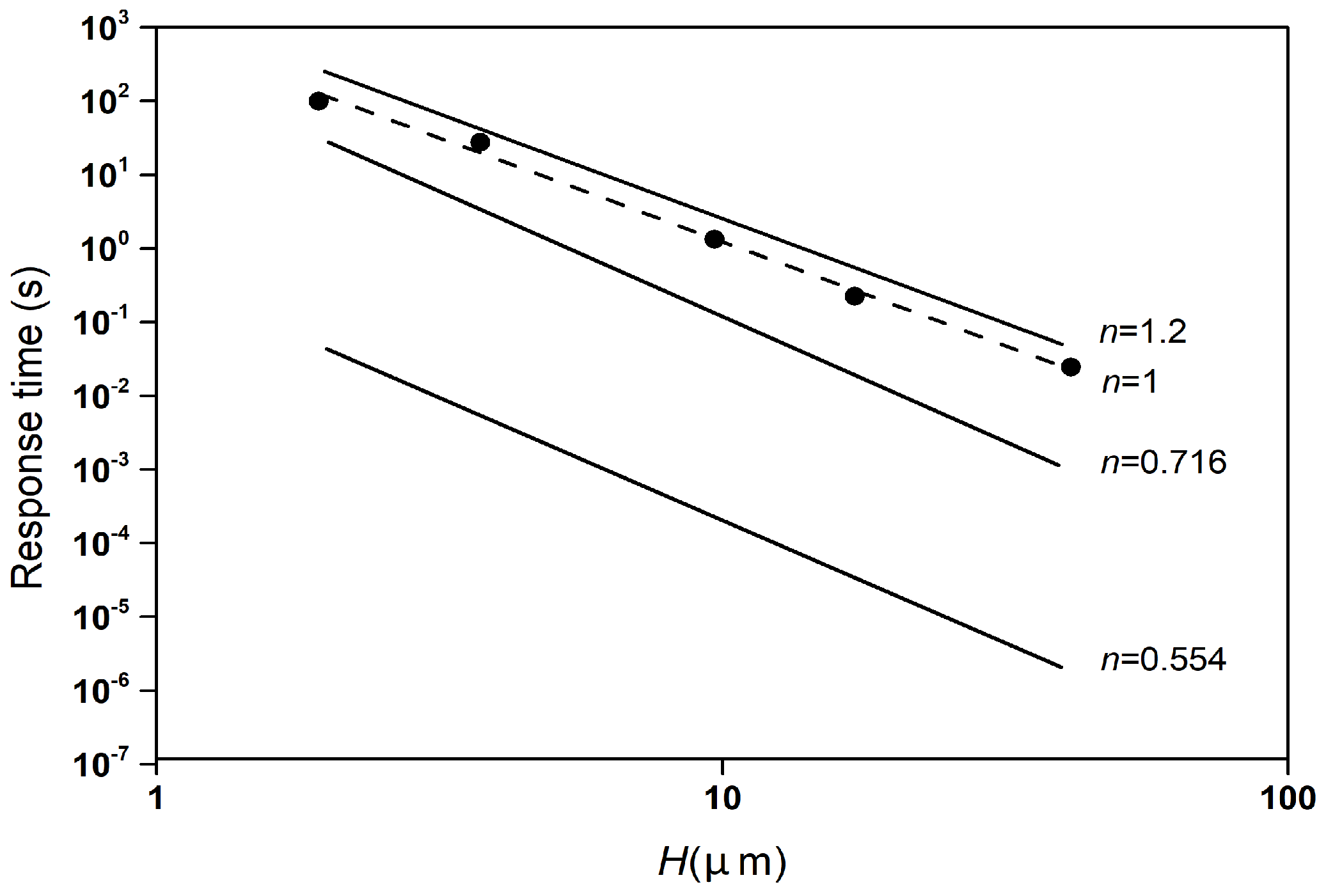
Figure 4 shows the dependence of the response time on channel height for n = 1 as predicted by the model (dashed line). The results are compared with Dendukuri et al.’s [24] experimental data for H = 2 , 10, 20 and 40 μ m (filled dots). The model reproduces the experimental linear trend with a 3 s μ m 1 slope. Increasing the channel width causes a reduction in the recovery stress of the channel elastic wall, with a consequent increase in the response time. In this case, the model prediction matches the experimental data with a RMSE of less than about 10%. The response times for the pseudoplastic and dilatant fluids as predicted by the model are also depicted (solid lines). As for the n = 1 case, the response time also decreases with H for a power-law fluid. In particular, for the dilatant case ( n = 1.2 ) the linear decrease closely follows a 3 s μ m 1 slope, while for the pseudoplastic fluids ( n = 0.554 and 0.716), the linear decrease follows a 2.82 s μ m 1 slope. However, compared to the Newtonian and dilatant power-law fluids, the response time for the n = 0.554 pseudoplastic fluid is reduced by about four orders of magnitude, while for the n = 0.716 case, the reduction is approximately of an order of magnitude. In passing, we note that the response time experienced by the dilatant fluid is only slightly longer than the one experienced by the Newtonian ( n = 1 ) fluid. As the channel height is reduced, the response time of the system increases. This occurs because in channels of a smaller height, there is a greater flow resistance that the fluid must overcome when it is flushed away from the channel.
The effects of the channel length on the wall response time are displayed in Figure 5. For n = 1 , the response times also fit the experimental data for varying channel lengths (i.e., 0.25, 0.5, 1 and 1.2 cm), all with a constant channel width of 200 μ m, height of 10 μ m and pressure 3 psi. The response time for both the Newtoninan and the dilatant fluid increases linearly following a 2 s μ m 1 slope. No difference is actually observed between both trends. In contrast, for the pseudoplastic fluids, the response time also increases linearly but this time with a 3.25 s μ m 1 slope for n = 0.716 and 3 s μ m 1 for n = 0.554 . Moreover, compared to the Newtonian and dilatant fluids, the response times for the pseudoplastic fluids are an order of magnitude smaller than for the former cases. As expected, the response time is always seen to increase with the length of the channel. The shorter wall response times shown by the pseudoplastic fluids ( n = 0.554 and 0.716) in Figure 4 and Figure 5 compared to the Newtonian ( n = 1 ) and dilatant fluids ( n = 1.2 ) may be due to the fact that the former fluids lower their viscosity when subjected to large shear rates.
The dependence of the response time on the applied pressure at the entrance of the channel for the Newtonian fluid (dashed line) as compared with the experimental data of Dendukuri et al. [24] (filled dots) is shown in the top-left frame of Figure 6. In fair agreement with the experimental measurements, the response time is almost invariant to changes in the applied pressure. The experimental data exhibit scattered values of the response time about the predicted line with small departures from it. Despite the scatter of the experimental data, the actual RMSE distance between the predicted values and the experimental measurements is less than 1 %. This also evidences an approximate invariance with the applied pressure. In general, this behavior is expected in situations where the height deformation is small. However, a pressure increase above 15 psi causes significant deformation in the channel walls, which in turn causes an increase in the channel wall recovery elastic stress. This elastic stress increase is compensated when a larger liquid volume is expelled. The balance between elastic and viscous forces causes the response time to be pressure-independent for small deformations. Finally, the response time changes as a function of the μ / E -ratio associated with the visco-elastic characteristics of the system. This means that if an oligomer of low viscosity is used, or a more rigid PDMS device is built, the response time will be consequently smaller.
The top-right, bottom-left and bottom-right frames of Figure 6 show the wall response time as a function of the applied pressure at the entrance of the channel for the n = 1.2 (dilatant) and the n = 0.716 and 0.554 (pseudoplastic) fluids, respectively. In particular, the response time for the dilatant fluid decreases as the pressure is increased and is about an order of magnitude higher than that experienced by the Newtonian fluid at low pressures. For the pseudoplastic fluids ( n = 0.716 and 0.554), the response time is from two to five orders of magnitude shorter than for the Newtonian case. The response time follows a trend similar to that displayed by the dilatant fluid, with larger values at low pressures. However, the differences between low and high pressures is so small that in general the response time for these fluids can be considered to remain almost invariant with pressure.
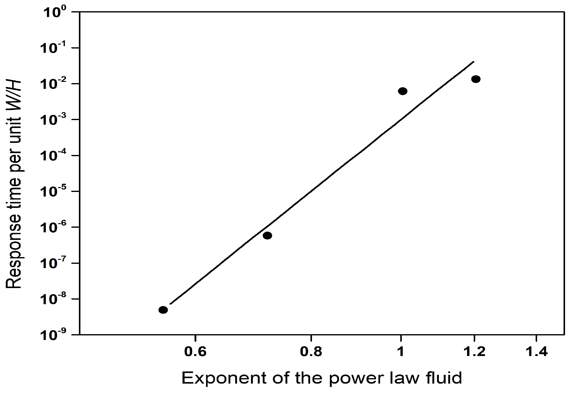
The predicted response time per unit applied pressure as a function of the exponent of the power-law fluid model (solid line) is shown in Figure 7. The predicted values match very well with the experimental data for n < 1 with negligible relative errors. For n = 1 , the predicted value differs from the experimental measurement by a relative error of 19 %. The worst case occurs for n = 1.2 , where the error grows to 66 %. The response time increases exponentially for power-law fluids with n > 1 and is very sensitive to changes in the fluid viscosity. On the other hand, Figure 8 shows the functional dependence of the response time on the channel width to height ratio, W / H . In general, the response time increases linearly with increasing the W / H ratio. In all cases, the linear increase has an approximate 2.5 s slope as a result of the reduction in the deformation curvature of the channel rectangular area. The response times of the Newtonian and dilatant fluids are similar and converge to the same values at high values of the W / H ratio. For the pseudoplastic fluids, however, the response times are about four ( n = 0.716 ) and six ( n = 0.554 ) orders of magnitude lower than those of the Newtonian and dilatant fluids. Moreover, the functional dependence of the model computed response time per unit W / H ratio on the exponent of the power-law fluid (solid line) is shown in Figure 9 as compared with experimental data from Dendukuri et al. [24] for n = 1 , Bird et al. [25] for n < 1 and present authors for n = 1.2 . Sharp variations for more than seven orders of magnitude occurs when the exponent changes from 0.554 (for a pseudoplastic fluid) to 1.2 (for a dilatant fluid). The best fit of the numerical data deviates from the model prediction by a RMSE of 0.016 , i.e., by approximately 1.6%.
Figure 10 shows the degree of deformation of the dimensionless channel height as a function of the dimensionless channel length for the power-law fluids analyzed for response times of 0.01 and 0.1 s and W / H ratios of 2.5 and 10. In particular, the top-left, top-right, bottom-left and bottom-right frames show the variation in the channel height for the n = 1 , n = 1.2 , n = 0.716 and n = 0.554 fluids, respectively. The model predicts a maximum deformation of 20% when the response time is 0.01 s and W / H = 10 , which is in line with Dendukuri et al.’s [24] and Gervais et al.’s [23] experimental data.
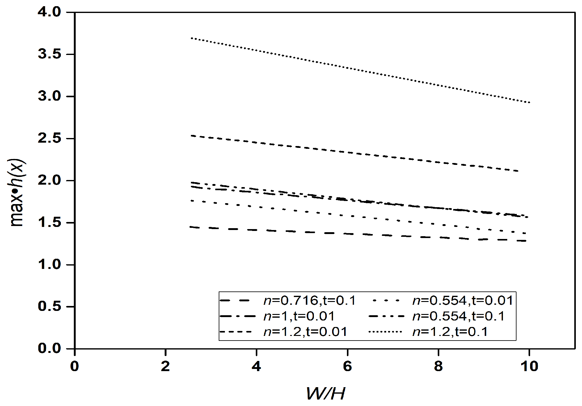
The variation in the deformation of the channel height with the W / H ratio is displayed in Figure 11 for all fluids analyzed and two different response times ( t = 0.01 and 0.1 s). In general, the height deformation decreases with increasing W / H ratios. Evidently, as the deformation area increases, the maximum channel deformation is reduced. Furthermore, the level of deformation increases with the response time. The model also predicts a dependence of the maximum deformation on the exponent of the power-law fluid. In particular, the dilatant ( n = 1.2 ) fluid causes a deformation, Δ h , from 2.5 to 3 times the non-deformed height, H, of the channel. On the other hand, the deformation for the Newtonian and pseudoplastic ( n = 0.716 ) fluids is from 0.2 to 0.8 times H, while for the n = 0.554 pseudoplastic fluid, the change is only from 0.12 to 0.6 times H. As opposed to pseudoplastic fluids, dilatant fluids become more viscous as more shear is applied. Therefore, they may cause an increase in the response time as they move slowly across the channel, thereby inducing a larger channel deformation. This could explain why the maximum height deformation is considerably larger for n > 1 .

4. Discussion

When analyzing separately the effects of the channel dimensions on the response time for different power-law fluids, we found that as the channel height increases, with all other geometric variables remaining constant, the response time decreases for all power-law fluids analyzed. However, the response time as a function of the type of fluid varies up to four orders of magnitude. This is due to changes in the flow resistance that must be overcome by the fluid when flushed out from the channel. This effect is better evidenced by the behavior of the response time as a function of the W / H ratio. As this ratio increases, the maximum height deformation decreases, causing the response time to increase.
It was also found that for power-law fluids with n 1 , the maximum channel deformations were of 16–80% of the initial height, while for fluids with n > 1 , the model-predicted deformation falls to between 2.5 and 3 times greater than the channel initial height. This is due to the influence of the fluid characteristics on the behavior of the fluid.
An increase in the exponent of the power-law fluid to n > 1 causes an increase in the response time as well as an increase in the maximum deformation of the channel height compared with a Newtonian fluid ( n = 1 ). This is because fluids with n > 1 move more slowly across the channel, thereby causing the response time and the stress of the fluid on the elastic wall of the channel to increase.
Finally, it is important to mention that the balance between the elastic forces on the wall and the viscous forces of the fluid ensures that the response time is independent of the stress applied to the fluid at the entrance of the channel, especially when the deformations are small so that the response time varies as a function of the W / H ratio. Rigid PDMS devices will allow making changes in the response time so as to reduce it to a minimum. This favors the use of channels with shorter lengths and larger flow stresses at the entrance (within mechanical stability limits). These are optimal characteristics to obtain a fast and dynamic response in the operation and design of a stop-flow lithography device. Therefore, the present results have practical implications in the development of pharmaceutical microfluidic devices. Other practical applications of these microfluidic systems may include nanoparticle preparation, drug encapsulation and delivery, culture and development of stem cells as well as cell analysis and diagnosis. In the biomedical field they can be used as micro-heat pumps and sinks, in DNA analysis, Lab-on-a-chip, urinary analysis and droplet generation among many other applications, while in chemical engineering, they are used as microreactors and in the synthesis of functional materials. Many other potential applications can be found in other fields such as, for example, medicine, food engineering, biology and chemistry.

5. Concluding Remarks

In this work, we have presented a simple model for the flow of power-law fluids in a rectangular channel with elastic ceiling. The model relies on momentum balance equations that can easily be analyzed using the lubrication approximation. Furthermore, this study allows us to assess separately the impact of the fluid type, the channel dimensions and the fluid stress at the entrance of the channel on the response time of deformation of the elastic ceiling of the rectangular channel.
The main results can be summarized as follows:
  • For a Newtonian fluid (with a power-law exponent n = 1 ), the model predicts the experimentally measured response times of wall channel deformation for different channel widths, heights and lengths with root-mean-square errors (RMSEs) less than ∼10%.
  • For pseudoplastic fluids ( n < 1 ), the deformation response times are from one to several orders of magnitude shorter than for Newtonian ( n = 1 ) and dilatant ( n > 1 ) fluids.
  • The maximum channel deformation and the time of flow residence are largely determined by the fluid power-law order and the width-to-height ratio of the elastic channel.
  • As a function of the channel width-to-height ratio, the largest maximum wall deformations are observed for the n = 1.2 fluid.
  • The solution methodology implemented here provides a lower bound to the non-linear problem and the results can be interpreted as a limiting case given by the lubrication approximation.
  • In spite of its simplicity, the present model can be used to study the behavior of non-Newtonian power-law fluids applied to the development of novel pharmaceutical microfluidic devices.

Author Contributions

Conceptualization, A.R.M., A.E.C.C. and N.A.N.M.; methodology, A.E.C.C. and M.P.D.; formal analysis, A.R.M. and M.P.D.; investigation, F.A.R. and C.A.V.; writing—original draft preparation, L.D.G.S. and A.R.M.; writing—review and editing, L.D.G.S.; visualization, F.A.R.; funding acquisition, C.A.V. All authors have read and agreed to the published version of the manuscript.

Funding

This research received no external funding.

Data Availability Statement

The data presented in this study are available on request from the corresponding author.

Acknowledgments

We acknowledge the Department of Basic Sciences of the Autonomous Metropolitan University, Azcapotzalco Campus for financial and technical support.

Conflicts of Interest

The authors declare no conflicts of interest.

Abbreviations

The following abbreviations are used in this manuscript:
HMicrochannel height ( μ m)
LMicrochannel length (cm)
WMicrochannel width ( μ m)
EYoung modulus (MPa and GPa)
ReReynolds number (dimensionless)
v Fluid velocity vector (m s 1 )
v x , v y , v z Fluid velocity components (cm s 1 )
pPressure (psi)
x , y , z Cartesian coordinates ( μ m)
T Stress tensor (kg m 1 s 2 )
I Identity tensor (dimensionless)
nPower-law exponent (dimensionless)
kPower-law constant (dyn s n cm 2 )
qDimensionless parameter
h ( x , t ) Deformation function of the microchannel ceiling ( μ m)
Δ h Height increase of microchannel ceiling ( μ m)
Δ h max Maximum height increase ( μ m)
t stop Time of flow residence in the channel (s)
t r Time of wall response (s)
t shutter Time to begin particle polymerization (s)
t f Time required to flush the particles out (s)
t rp Lower bound for the stop time (s)
Greek letters
μ Viscosity (mPa s)
σ Stress applied to produce the deformation (MPa)
ξ = σ / E Applied deformation (dimensionless)
σ ̲ ̲ Shear stress tensor (kg m 1 s 2 )
Ω = p / E Deformation of the channel ceiling (dimensionless)
Θ = h ( x ) / H Normalized deformation function (dimensionless)
ϵ = x / L Normalized position along the channel (dimensionless)

References

  1. Urban, D.; Takamura, K. (Eds.) Polymer Dispersions and Their Industrial Applications; Wiley-VCH: Hoboken, NJ, USA, 2002. [Google Scholar]
  2. Lu, Y.; Yin, Y.; Xia, Y. Three-dimensional photonic crystals with non-spherical colloids as building blocks. Adv. Mater. 2001, 13, 415–420. [Google Scholar] [CrossRef]
  3. Langer, R.; Tirrell, D.A. Designing materials for biology and medicine. Nature 2004, 428, 487–492. [Google Scholar] [CrossRef] [PubMed]
  4. Finkel, N.H.; Lou, X.; Wang, C.; He, L. Peer reviewed: Barcoding the microworld. Anal. Chem. 2004, 76, 352A–359A. [Google Scholar] [CrossRef] [PubMed]
  5. Pregibon, D.C.; Toner, M.; Doyle, P.S. Multifunctional encoded particles for high-throughput biomolecule analysis. Science 2007, 315, 1393–1396. [Google Scholar] [CrossRef] [PubMed]
  6. Steinbacher, J.L.; McQuade, D.T. Polymer chemistry in flow: New polymers, beads, capsules, and fibers. J. Polym. Sci. Part A Polym. Chem. 2006, 44, 6505–6533. [Google Scholar] [CrossRef]
  7. Kawakatsu, T.; Kikuchi, Y.; Nakajima, M. Regular-sized cell creation in microchannel emulsification by visual microprocessing method. J. Am. Oil Chem. Soc. 1997, 74, 317–321. [Google Scholar] [CrossRef]
  8. Thorsen, T.; Roberts, R.W.; Arnold, F.H.; Quake, S.R. Dynamic pattern formation in a vesicle-generating microfluidic device. Phys. Rev. Lett. 2001, 86, 4163–4166. [Google Scholar] [CrossRef]
  9. Shelley, A.L.; Bontoux, N.; Stone, H.A. Formation of dispersions using “flow focusing” in microchannels. Appl. Phys. Lett. 2003, 82, 364–366. [Google Scholar]
  10. Okushima, S.; Nisisako, T.; Torii, T.; Higuchi, T. Controlled production of monodisperse double emulsions by two-step droplet breakup in microfluidic devices. Langmuir 2004, 20, 9905–9908. [Google Scholar] [CrossRef]
  11. Utada, A.S.; Lorenceau, E.; Link, D.R.; Kaplan, P.D.; Stone, H.A.; Weitz, D.A. Monodisperse double emulsions generated from a microcapillary device. Science 2005, 308, 537–541. [Google Scholar] [CrossRef]
  12. Sugiura, S.; Nakajima, M.; Tong, J.; Nabetani, H.; Seki, M. Preparation of monodispersed solid lipid microspheres using a microchannel emulsification technique. J. Colloid Interface Sci. 2000, 227, 95–103. [Google Scholar] [CrossRef]
  13. Nisisako, T.; Torii, T.; Higuchi, T. Novel microreactors for functional polymer beads. Chem. Eng. J. 2004, 101, 23–29. [Google Scholar] [CrossRef]
  14. Dendukuri, D.; Tsoi, K.; Hatton, T.A.; Doyle, P.S. Controlled synthesis of nonspherical microparticles using microfluidics. Langmuir 2005, 21, 2113–2116. [Google Scholar] [CrossRef]
  15. Xu, S.; Nie, Z.; Seo, M.; Lewis, P.; Kumacheva, E.; Stone, H.A.; Garstecki, P.; Weibel, D.B.; Gitlin, I.; Whitesides, G.M. Generation of monodisperse particles by using microfluidics: Control over size, shape, and composition. Angew. Chem. 2005, 44, 724–728. [Google Scholar] [CrossRef]
  16. Nie, Z.; Xu, S.; Seo, M.; Lewis, P.C.; Kumacheva, E. Polymer particles with various shapes and morphologies produced in continuous microfluidic reactors. J. Am. Chem. Soc. 2005, 127, 8058–8063. [Google Scholar] [CrossRef]
  17. Nisisako, T.; Torii, T.; Takahashi, T.; Takizawa, Y. Synthesis of monodisperse bicolored Janus particles with electrical anisotropy using a microfluidic Co-Flow system. Adv. Mater. 2006, 18, 1152–1156. [Google Scholar] [CrossRef]
  18. Shepherd, R.F.; Conrad, J.C.; Rhodes, S.K.; Link, D.R.; Marquez, M.; Weitz, D.A.; Lewis, J.A. Microfluidic assembly of homogeneous and Janus colloid-filled hydrogel granules. Langmuir 2006, 22, 8618–8622. [Google Scholar] [CrossRef] [PubMed]
  19. Dendukuri, D.; Hatton, T.A.; Doyle, P.S. Synthesis and self-assembly of amphiphilic polymeric microparticles. Langmuir 2007, 23, 4669–4674. [Google Scholar] [CrossRef] [PubMed]
  20. Decker, C.; Jenkins, A.D. Kinetic approach of oxygen inhibition in ultraviolet-and laser-induced polymerizations. Macromolecules 1985, 18, 1241–1244. [Google Scholar] [CrossRef]
  21. Glotzer, S.C. Some assembly required. Science 2004, 306, 419–420. [Google Scholar] [CrossRef] [PubMed]
  22. Dendukuri, D.; Pregibon, D.C.; Collins, J.; Hatton, T.A.; Doyle, P.S. Continuous-flow lithography for high-throughput microparticle synthesis. Nat. Mater. 2006, 5, 365–369. [Google Scholar] [CrossRef] [PubMed]
  23. Gervais, T.; El-Ali, J.; Günther, A.; Jensen, K.F. Flow-induced deformation of shallow microfluidic channels. Lab Chip 2006, 6, 500–507. [Google Scholar] [CrossRef] [PubMed]
  24. Dendukuri, D.; Gu, S.S.; Pregibon, D.C.; Hatton, T.A.; Doyle, P.S. Stop-flow lithography in a microfluidic device. Lab Chip 2007, 7, 818–828. [Google Scholar] [CrossRef]
  25. Bird, R.B.; Steward, W.E.; Lightfoot, E.N. Transport Phenomena; Wiley: Hoboken, NJ, USA, 2006. [Google Scholar]
  26. Hayes, R.E.; Dannelongue, H.H.; Tanguy, P.A. Numerical simulation of mold filling in reaction injection molding. Polym. Eng. Sci. 1991, 31, 842–848. [Google Scholar] [CrossRef]
  27. Anand, V.; Christov, I.C. Revisiting steady viscous flow of a generalized Newtonian fluid through a slender elastic tube using shell theory. J. Appl. Math. Mech./Z. Angew. Math. Mech. 2021, 101, e201900309. [Google Scholar] [CrossRef]
  28. Inamdar, T.C.; Wang, X.; Christov, I.C. Unsteady fluid–structure interactions in a soft-walled microchannel: A one-dimensional lubrication model for finite Reynolds number. Phys. Rev. Fluids 2020, 5, 064101. [Google Scholar] [CrossRef]
  29. Anand, V.; David, J.; Christov, I.C. Non-Newtonian fluid–structure interactions: Static response of a microchannel due to internal flow of a power-law fluid. J. Non-Newton. Fluid Mech. 2019, 264, 62–72. [Google Scholar] [CrossRef]
  30. Skotheim, J.M.; Mahadevan, L. Soft lubrication. Phys. Rev. Lett. 2004, 92, 245509. [Google Scholar] [CrossRef]
Figure 1. Schematic representation of the deformation of the rectangular microchannel as a result of a given flow. (A) Frontal cross-sectional view and (B) lateral view of the microchannel.
Fluids 09 00077 g001
Figure 2. Schematic representation of the deformed channel under a circulating flow.
Fluids 09 00077 g002
Figure 3. Predicted wall response time for the n = 1 fluid as a function of the channel width for a constant pressure of 3 psi, channel length of 1 cm and channel height of 200 μ m (dashed line) as compared with Dendukuri et al.’s [24] experimental measurements (filled dots).
Fluids 09 00077 g003
Figure 4. Dependence of the wall response time on the channel height for a constant pressure of 3 psi, a channel length of 1 cm and a channel width of 200 μ m. The dashed line describes the tendency of the Newtonian case, which is compared with the experimental data of Dendukuri et al. [24] for n = 1 . The solid lines depict the dependence of the n = 1.2 , 0.716 and 0.554 power-law fluids.
Fluids 09 00077 g004
Figure 5. Dependence of the wall response time on the channel length for a constant pressure of 3 psi, a channel height of 10 μ m and a channel width of 200 μ m. The dashed line describes the dependence of the Newtonian case, which is compared with the experimental data of Dendukuri et al. [24] for n = 1 . The solid lines depict the dependence of the n = 1.2 , 0.716 and 0.554 power-law fluids.
Fluids 09 00077 g005
Figure 6. Dependence of the wall response time on the applied pressure at the entrance of the channel for the n = 1 (top left), n = 1.2 (top right), n = 0.716 (bottom left) and n = 0.554 (bottom right) fluids for constant channel height, width and length of 10 μ m, 200 μ m and 1 cm, respectively. The dots displayed in the top-left frame corresponds to Dendukuri et al.’s [24] experimental data.
Fluids 09 00077 g006
Figure 7. Predicted response time per unit applied pressure (in psi) as a function of the exponent of the power-law fluid model (solid line) as compared with experimental data obtained from Dendukuri et al. [24] for n = 1 , Bird et al. [25] for n = 0554 and 0.716 and present authors for n = 1.2 (filled dots).
Fluids 09 00077 g007
Figure 8. Wall response time against the channel width to height ratio for all power-law fluid models considered.
Fluids 09 00077 g008
Figure 9. Predicted wall response time per unit W / H ratio against the exponent of the power-law fluid model (solid line) as compared with experimental data from Dendukuri et al. [24] (for n = 1 ), Bird et al. [25] (for n < 1 ) and present authors (for n = 1.2 ) (filled dots).
Fluids 09 00077 g009
Figure 10. Relationship between the dimensionless channel height and the dimensionless channel length for the n = 1 (top left), n = 1.2 (top right), n = 0.716 (bottom left) and n = 0.554 (bottom right) fluids for varied wall response times ( t = 0.01 and 0.1 s) and W / H ratios (2.5 and 10).
Fluids 09 00077 g010
Figure 11. Maximum height deformation of the channel as a function of the W / H ratio for all fluids analyzed and two different response times (i.e., t = 0.01 and 0.1 s).
Fluids 09 00077 g011
Disclaimer/Publisher’s Note: The statements, opinions and data contained in all publications are solely those of the individual author(s) and contributor(s) and not of MDPI and/or the editor(s). MDPI and/or the editor(s) disclaim responsibility for any injury to people or property resulting from any ideas, methods, instructions or products referred to in the content.

