Article

Numerical Study of Rarefied Gas Flow in Diverging Channels of Finite Length at Various Pressure Ratios

1
Institute for Technical Physics, Karlsruhe Institute of Technology, 76344 Eggenstein-Leopoldshafen, Germany
2
Department of Mechanical Engineering, University of West Attica, 12241 Athens, Greece
*
Author to whom correspondence should be addressed.
Fluids 2024, 9(3), 78; https://doi.org/10.3390/fluids9030078
Submission received: 16 February 2024 / Revised: 8 March 2024 / Accepted: 13 March 2024 / Published: 19 March 2024
(This article belongs to the Special Issue Rarefied Gas Flows: From Micro-Nano Scale to Hypersonic Regime)

Abstract

:
In the present work, the gas flows through diverging channels driven by small, moderate, and large pressure drops are studied, considering a wide range of the gas rarefaction from free molecular limit through transition flow regime up to early slip regime. The analysis is performed using the Shakhov kinetic model, and applying the deterministic DVM method. The complete 4D flow problem is considered by including the upstream and downstream reservoirs. A strong effect of the channel geometry on the flow pattern is shown, with the distributions of the macroscopic quantities differing qualitatively and quantitatively from the straight channel flows. The mass flow rate data set from the complete solution is compared with the corresponding set obtained from the approximate kinetic methodology, which is based on the fully developed mass flow rate data available in the literature. In addition, the use of the end-effect approach significantly improves the applicability range of the approximate kinetic methodology. The influence of the wall temperature on the flow characteristics is also studied and is found to be strong in less-rarefied cases, with the mass flow rate in these cases being a decreasing function of the temperature wall. Overall, the present analysis is expected to be useful in the development and optimization of technological devices in vacuum and aerospace technologies.

1. Introduction

Studying and describing internal gas flows is important in a wide range of scientific and engineering fields, serving an essential function in advancing multiple technological uses. The Knudsen number is a crucial dimensionless factor in the analysis of internal gas flows. It represents the ratio of the average distance traveled by gas molecules between collisions to the characteristic size of a system. The Knudsen number acts as an important guide for selecting modeling equations based on the specific characteristics of the gas flow regime. Based on this, different flow regimes are defined. The continuum flow regime, with the mean free path being significantly smaller than the characteristic dimension of the system, refers to low values of the Knudsen number (lower than 0.001). In the continuum flow regime, Navier–Stokes equations are easily applicable. The transitional flow regime occurs when the Knudsen number ranges from 0.1 to 10, where the traditional Navier–Stokes equations are no longer applicable. At high Knudsen number values (greater than 10), where the gas state is characterized by long molecular mean free paths, a free molecular regime is observed. The Boltzmann kinetic equation [1], which offers an accurate description of the microscopic gas behavior, connecting individual molecular interactions to macroscopic properties, can be applied in the whole range of the Knudsen number.
In recent years, there has been a significant focus on examining internal gas flows through the application of Boltzmann’s kinetic equation, mainly using the Direct Simulation Monte Carlo method (DSMC) [2] and the Discrete Velocity Method (DVM) [3]. The literature in this area is extensive, and only some examples are provided here. A substantial body of work has been done in studying internal gas flows through straight channels. In the literature, numerous publications analyze such flows in a wide range of the Knudsen number, covering both small and large pressure ratios, as well as channels of various cross-sections. S. Varoutis et al. [4,5] conducted research on internal gas flows in circular channels of finite length covering a variety of the Knudsen numbers related to vacuum systems. In addition, F. Sharipov and D. V. Kozak [6] utilized the DSMC method, while I. Graur et al. [7] used the DVM method to analyze rarefied gas flows through a slit into vacuum. A considerable amount of research has also been conducted on the analysis of internal gas flows in long channels [8,9,10,11].
There is substantial interest in studying gas flows through diverging or converging channels due to their extensive range of applications. The study of internal gas flows within diverging channels finds widespread application in the field of aerodynamics, influencing the design and performance of various engineering systems. Diverging channels play a significant role in the field of aerospace engineering [12,13,14] and wind tunnel design [15]. Also, simulations of internal gas flow in channels play a crucial role in various applications within vacuum technology, contributing to the efficiency and functionality of systems such as fusion reactors, vacuum pumps, and Knudsen pumps [16,17]. A more extensive literature review can be found in O. Sazhin and A. Sazhin’s work [18].
The examination of internal gas flows through diverging channels across the entire range of the gas rarefaction has been typically carried out using the Direct Simulation Monte Carlo method, particularly employing implicit boundary conditions [19,20,21,22]. Recent research conducted by G. Tatsios et al. [23] indicates that implicit boundary conditions result in certain deviations; hence, it is crucial to acquire a complete solution with significant regions at both ends of the channel. Additionally, the flow in diverging channels for axisymmetric and plate geometries has been thoroughly studied in the works of V.A. Titarev et al. [24] and O. Sazhin and A. Sazhin [18], respectively, focusing on flows into a vacuum. In these studies, the complete solution was introduced, and the significant impact of the existence of the upstream and downstream reservoirs on the calculation of the flow parameters was demonstrated. The importance of the existence of the reservoirs in the solution was also highlighted by A. Yakunchikov and V. Kosyanchuk [25] in the case of rarefied gas flow through a straight channel using the Event-Driven Molecular Dynamics (EDMD) method. The present work aims to reduce discrepancies in the literature through the following three aspects: The initial goal is to study the characteristics of the gas flows through diverging channels over a wide range of gas rarefaction, geometric parameters, and various pressure ratios by applying the complete flow set-up. To the best of the authors’ knowledge, an extensive kinetic database on the mass flow rate for this flow set-up is not yet available in the literature. The second objective is to examine the validity range of a simple kinetic approach based on the simplifications directly expressed by the fully developed theory [26]. In [24] it has been demonstrated that this approach does not perform optimally in the case of flows into vacuum. The third objective is to thoroughly study the effect of the wall temperature in the case of the gas flows through diverging channels considering the complete solution. Ιn [27], a significant effect of the wall temperature on the flow field quantities in straight channels was demonstrated.
This paper is organized as follows: In Section 2, the flow configuration and the main flow parameters are described. In Section 3, the applied kinetic approaches are described and validated against available numerical data in the literature. In Section 4, the numerical results are presented and discussed, and in Section 5, the main conclusions that have been drawn so far are pointed out.

2. Flow Configuration

A schematic diagram of the examined flow configuration is shown in Figure 1a. The flow set-up consists of two large reservoirs connected by a diverging channel with dimensions of length L , width W , and height H x , with the height increasing linearly in the flow direction. The height of the channel at a certain distance from the inlet is defined as H x = H o u t H i n / L x + H i n , where H i n and H o u t denote the channel height at the inlet and outlet, respectively. The width of the channel is assumed to be considerably larger compared to its height, i.e., W H x . The two reservoirs are maintained at different pressures, namely P A and P B , with P A > P B , while the temperature of the gas at the two reservoirs is assumed constant and equal to T 0 . The channel wall temperature T W is also kept constant and uniform along the wall (see Figure 1a, along the dash–dotted line). Due to the flow symmetry, only half of the flow domain is considered, i.e., y > 0 . Under steady-state conditions, a flow from the high-pressure reservoir towards the low-pressure reservoir is established. In order to make the presentation of the numerical results more compact, their non-dimensional form is chosen. The macroscopic quantities, such as the number density n , the temperature T , the pressure P , the velocity vector u = u x , u y , and the heat flux vector q = q x , q y , are normalized as follows:
n ~ x ~ , y ~ = n x , y n A , T ~ x ~ , y ~ = T x , y T 0 , P ~ x ~ , y ~ = P x , y P A , u ~ x ~ , y ~ = u x , y υ 0 , q ~ x ~ , y ~ = q x , y P A υ 0 ,  
where υ 0 = 2 k B T 0 / m is the most probable speed, with k B being the Boltzmann constant and m being the gas molecular mass. Τhe x and y coordinates are normalized as x ~ = x / H i n and y ~ = y / H i n , respectively.
The state of the gas flow can be described by the following five dimensionless quantities:
  • The reference rarefaction parameter δ 0 , defined as
    δ 0 = P A H i n μ 0 υ 0 ,
    where μ 0 is the gas viscosity at the reference temperature T 0 . The rarefaction parameter δ 0 is proportional to the inverse Knudsen number;
  • The dimensionless channel length λ = L / H i n ;
  • The ratio of channel height at the two channel ends η = H o u t / H i n ;
  • The pressure ratio φ = P B / P A ;
  • The temperature ratio τ = T W / T 0 .
The gas mass flow rate M ˙ through the channel is the computational parameter of great practical importance, and its dimensionless form is defined as
M ~ = M ˙ M ˙ 0 ,
where M ˙ 0 = P A H i n / π υ 0 is the dimensional mass flow rate in the case of flow through slit ( λ = 0 ) assuming flow into the vacuum ( P B = 0 ) and free molecular flow conditions. It is noted that the normalization for the mass flow rate has been chosen in order to facilitate comparisons with already published data in the literature for some limit cases, such as that of gas flows through straight channels [28]. In the present work, the dependence of the flow quantities (dimensionless mass flow rate and dimensionless macroscopic quantities) on the five flow parameters, namely, δ 0 , λ , η , φ , and τ , is determined and discussed.

3. Kinetic Approaches

3.1. Complete 4D Kinetic Solution

In the complete kinetic solution, the simulation domain includes the channel region as well as part of the area of the two reservoirs. Due to the fact that in real applications, the reservoir size can be significantly larger compared to the channel size, for the sake of reducing the required computational effort, it is a standard practice in this type of flow to extend the computational domain in the reservoirs until a solution that is independent of the size of these computational regions is found. As shown in Figure 1a, where the computational area is highlighted in gray, the computational domain is extended by H A and L A inside the high-pressure reservoir, as well as by H B and L B inside the low-pressure reservoir. In the present work, the sizes of the simulation regions inside the high- and low-pressure reservoir were chosen as H A , L A = 30 H i n , 30 H i n and H B , L B = 20 H o u t , 20 H o u t , respectively. Additional simulations showed that by doubling the size of these regions, the changes in the calculated macroscopic quantities remain smaller than 1%.
The flow characteristics are analyzed on the basis of the Shakhov kinetic model [29]. The Shakhov kinetic model is considered one of the most widely used kinetic models in the study of isothermal (e.g., [8,23,24,30,31,32,33]) and non-isothermal (e.g., [34,35,36,37,38,39,40,41]) gas flows in the whole range of the gas rarefaction, and its reliability has been demonstrated by performing comparisons with available experimental measurements [42,43,44,45] and DSMC data [46,47,48,49]. The Shakhov model, in its applied form, recovers both shear viscosity and thermal conductivity simultaneously and it fulfills all the collision invariants. For the flow problem under question, the Shakhov governing equations in terms of the dimensionless quantities (1) can be written as [7,50,51]:
t ~ h g + c x ~ x ~ h g + c y ~ y ~ h g = δ 0 n ~ T ~ 1 ω h s g s h g ,
where c = c x ~ , c y ~ is the dimensionless molecular velocity vector, which in dimensional form reads as ξ = c x ~ υ 0 , c y ~ υ 0 , t ~ = t υ 0 / H i n is the dimensionless time variable, and ω is the viscosity index, with its two limit cases being 0.5 for hard-sphere molecules and 1 for Maxwell molecules. In Equation (4), h x ~ , y ~ , c x ~ , c y ~ and g x ~ , y ~ , c x ~ , c y ~ are the reduced dimensionless distribution functions, which are defined as h , g = 1 , c z ~ 2 f ~ d c z ~ , with f ~ = f n A / υ 0 3 being the dimensionless velocity distribution function. The dimensional distribution function f is defined in such a way that f d ξ d r represents the number of particles in the volume element d r = d x d y d z around the position vector r with velocity in d ξ = d ξ x d ξ y d ξ z around ξ at time t . Additionally, in Equation (4), the relaxing Shakhov distribution functions, h s and g s , are read as:
h s g s = n ~ π T ~ exp c u ~ 2 T ~ 1 + 4 15 n ~ T ~ 3 q ~ c u ~ c u ~ 2 2 T ~ n ~ 2 π exp c u ~ 2 T ~ 1 + 4 15 n ~ T ~ 3 q ~ c u ~ c u ~ 2 T ~ ,
where c u ~ 2 = c x ~ u ~ x ~ 2 + c y ~ u ~ y ~ 2 and q ~ c u ~ = q ~ x ~ c x ~ u ~ x ~ + q ~ y ~ c y ~ u ~ y ~ . The macroscopic quantities of practical interest can be calculated as moments of the distribution functions ( h and g ) as follows:
n ~ u ~ x ~ u ~ y ~ T ~ q ~ x ~ q ~ y ~ = h c x ~ h / n ~ c y ~ h / n ~ 2 c u ~ 2 h + g / 3 n ~ c x ~ u ~ x ~ c u ~ 2 h + g c y ~ u ~ y ~ c u ~ 2 h + g d c x ~ d c y ~ .
A complete kinetic formulation requires the definition of the boundary conditions. In the modeling along the open boundary lines (shown with dashed lines in Figure 1a) in the high-pressure reservoir, the particles enter the computational area at the reservoir conditions with their incoming distribution functions ( h A + , and g A + ) defined as
h A + g A + = 1 π exp c x ~ 2 c y ~ 2 1 2 π exp c x ~ 2 c y ~ 2 ,
Also, particles enter the computational domain along the open boundary lines in the low-pressure reservoir at the corresponding conditions with their incoming distribution functions ( h B + , and g B + ) defined as
h B + g B + = φ h A + g A + .
Diffuse boundary conditions are applied along the solid walls (shown with solid and dash–dotted lines in Figure 1a). According to the diffuse molecular scattering, the distribution functions of the particles emitted from the walls are expressed as
h W + g W + = n ~ W π τ exp c x ~ 2 c y ~ 2 τ n ~ W 2 π exp c x ~ 2 c y ~ 2 τ ,
where n ~ W is calculated from the no-penetration condition (by imposing zero normal velocity) at the walls. In addition, symmetry boundary conditions are imposed along the x -axis.
As can be easily observed from Equations (4)–(6), the study of the considered flow set-up involves the solution of a 4D kinetic problem (2D in the velocity space and 2D in the physical space). The system of the two kinetic Equations (4) and (5) in conjunction with the moments (6) and the boundary conditions (7)–(9) is solved by applying the Discrete Velocity Method (DVM). The deterministic DVM method is nowadays considered the widely accepted numerical technique by the research community for solving kinetic equations and describing heat, mass, and momentum transfer phenomena in the whole range of gas rarefaction (e.g., [52,53,54,55,56,57,58,59,60]). The literature survey is very extensive, and for this reason, only a brief description of the method is provided here, focusing on the numerical details concerning the present flow problem. In the velocity space, the continuum spectrum of the molecular velocity c x ~ , c y ~ , is replaced by a set of 24 points in each direction (576 points in total), which have been chosen as the abscissas of the Gauss–Hermite rule. Following our previous work [51], in which successful extensive comparisons with the DSMC method were performed, the physical space is discretized by applying the DUGKS (discrete unified gas kinetic scheme) cell-centered finite-volume scheme. For further details regarding the applied DUGKS kinetic scheme, the reader should refer to [61,62,63], where a very comprehensive description of the DUGKS kinetic scheme is provided. The kinetic solution in physical space is achieved using a non-uniform triangular mesh. The applied mesh was constructed with the open-source SALOME meshing suite [64]. An illustrative picture of the mesh is shown in Figure 1b. As it is seen, the grid remains dense in the regions near the inlet and outlet of the channel and becomes even denser inside the channel and close to the solid walls where rapid changes in the macroscopic quantities are expected. More specifically, the minimum and the maximum dimensionless cell size inside the channel are set as 0.03 and 0.06, respectively. The size of the mesh depends on the geometrical characteristics, such as λ and η , with the number of elements varying between 40,000 ( λ = 1 and η = 2 ) and 80,000 ( λ = 10 and η = 5 ). The discretized equations are solved in an iterative manner for a given time step, chosen such that the maximum Courant–Friedrichs–Lewy number at each time step is 0.8. We assumed that convergence was achieved, when the maximum relative difference in the local macroscopic quantities between two successive iteration steps is less than 10−12. After the simulation reaches steady state, the maximum difference between the dimensionless mass flux values at the inlet and outlet is less than 2%. The suitability of the before-mentioned choices of the numerical parameters was checked by performing indicative test simulations with a higher number of molecular velocity points (×2 the number of discrete velocities) and denser grids (×2 the number of grid elements), with the maximum observed deviation in terms of the mass flow rate and the other macroscopic quantities being less than 0.8%. Overall, the choice of the numerical parameters ensures a numerical uncertainty of the provided data within 2%. The simulations were performed on a local cluster (CALIPSO) consisting of 16 nodes and each node was equipped with 2 Intel® Xeon® CPUs (E5-2660 v2 @ 2.20GHz). The simulation time varied from some hours in the case of small δ 0 , up to several weeks for the most computationally demanding cases of large values of δ 0 , λ , and η .
To assess the validity of our numerical implementation, comparisons were performed with the available and generally accepted DSMC data in the literature for the flows through straight channels under large and moderate pressure ratio drops [28], as well as for diverging channel flows into vacuum [18]. The comparison is shown in Table 1 in terms of the dimensionless mass flow rate M ~ considering moderate ( φ = 0.5 ) and large ( φ = 0 ) pressure ratios, as well as three indicative values of the gas rarefaction parameter δ 0 = 0.1,1 , 10 . The results are in very good agreement, with the maximum deviation remaining less than 2%. It is pointed out, that this small deviation remains within the numerical uncertainty adopted in the present work and it can be considered as an acceptable deviation between DSMC and DVM.

3.2. Approximate Kinetic Approach

A simplified kinetic approach, which is based on the long capillary theory that allows fast calculations of the mass flow rate, was proposed in [65]. Later on, this approach was extended to the case of flows through tubes of variable cross-sections [66], while in [26], this methodology was also applied to simulate rarefied gas flows through channels of variable rectangular cross-sections. In this work, the same methodology is also applied to the flow problem under question to investigate its applicability margins by performing comparisons with the complete solution given in Section 3.1. Hence, only a short description of this approximate kinetic approach is provided here. According to this simplified approach, as long as the channel is long enough and the local pressure gradient in the flow direction remains small, the flow inside the channel at any cross section can be described by the linear fully developed theory. The computational time needed to simulate one cross-section with the linear fully developed approach is negligible compared to that required for the complete solution described in Section 3.1. This approach consists of the following three steps: (1) the gas rarefaction level at the inlet and outlet of the channel is determined by calculating the values of the rarefaction parameter δ i n and δ o u t based on the pressure values P A and P B , the gas properties (viscosity), and the geometrical characteristics (the heights H i n and H o u t ); (2) the fully developed solution (the dimensionless reduced flow rate G P δ x [26,67]) is obtained for a wide range of the local gas rarefaction parameter δ x according to δ x δ i n , δ o u t ; and (3) calculating the mass flow rate by solving numerically the following mass balance differential equation:
P ~ x = L M ~ H i n π G P H i n H x 2 ,
where P ~ x = P x / P A and x = x / L . The values for G P δ x were obtained by applying our already validated, fully developed flow code from [67]. The ordinary differential Equation (10) is solved in an iterative manner. More specifically, the initial value problem, described by Equation (10) and the initial condition P ~ 0 = 1 is solved iteratively using Euler’s method until the value of the mass flow rate M ~ that leads to the actual value of the outlet pressure ( P ~ 1 = φ ) is found. The iteration process is repeated until the absolute difference between the actual and the estimated value of the pressure is less than 10−8. The numerical solution is obtained using 4000 intervals equally spaced along the x -axis. In Table 2, a comparison between our data and the corresponding ones in [26] is performed for various values of δ 0 and φ with η = 10 . As demonstrated, the maximum deviation remains less than 1%, confirming the validity of our numerical code.

4. Results and Discussion

The present analysis covers a wide range of the involved flow paramters. More specifically, the study was carried out for moderate ( η = 2 ) and large values ( η = 5 ) of the aspect ratio η , for three pressure ratios φ = 0.1,0.5,0.8 corresponding to small ( φ = 0.8 ), moderate ( φ = 0.5 ), and large pressure drops ( φ = 0.1 ), while the rarefaction parameter varies from 0 up to 10, representing gas flows from free molecular regime up to early slip regime. In addition, three indicative values of the dimensionless channel length, namely, λ = 1,5 , 10 , and two values of the temperature ratio τ , namely, τ = 1,3.3 , were considered.
This section is organized into two subsections. In Section 4.1, the results for the isothermal case of τ = 1 are presented, and the validity of the approximate kinetic approach (Section 3.2) is investigated, while in Section 4.2, the analysis is focused on the effect of the temperature ratio τ on the flow characteristics.

4.1. Isothermal Case

Table 3 shows the hard-sphere values of the dimensionless mass flow rate M ~ for various combinations of δ 0 , φ , λ , and η . As expected, in all cases, the increase in the pressure ratio φ (or decrease in the pressure drop), which is the driving force of the studied gas flow, causes a significant decrease in the mass flow rate. Depending on the level of the gas rarefaction, as the pressure ratio φ increases from 0.1 to 0.8, the dimensionless mass flow rate M ~ can be reduced by 49–78%. As observed, the geometry parameters λ and η have a significant effect on M ~ . In general, the mass flow rate increases either by decreasing the dimensionless length λ or by increasing the aspect ratio η . This behavior is justified by the fact that by increasing the dimensionless length or decreasing the aspect ratio, the wall effects become more pronounced, enhancing the wall resistance to the induced flow. The effect of the geometry parameters λ and η on M ~ remains significant for all examined pressure ratio values. In quantitative terms, the increase in the aspect ratio η from 2 to 5 (2.5 times) causes an increase in M ~ by about 1.07–1.09, 1.5–1.9, and 1.7–2.3 times in the case of λ = 1 , 5 and 10, respectively. By comparing the present results for the plane geometry with those in [24], which considers conical pipes, we can conclude that for similar pressure ratio conditions, a similar effect of the aspect ratio η on M ~ is observed. This means that when fast engineering calculations are required, the mass flow rate through diverging conical pipes for pressure ratios different than zero (which are not considered here since the plane geometry is studied) may be estimated, as a rough approximation, by using the available data in literature for straight tubes and modifying them considering the effect of the aspect ratio η on M ~ reported in this work for the plane geometry. However, when accuracy is important, the modeling of the flow through diverging conical pipes is required and suggested.
The data for λ = 10 , given in Table 3, confirm the existence of a shallow Knudsen minimum for the case of small values of the aspect ratio η = 2 , as well as for all values of the pressure ratio φ . However, as the channel becomes more open (higher aspect ratio η ), no Knudsen minimum is observed even for the longest considered channels with λ = 10. It is noted that, also in [18], the authors observed the Knudsen minimum for the same values of λ and η assuming φ = 0 . However, for the shorter channels with λ < 10 and for all considered values of η , following the behavior previously reported in [28] for the straight channels, the dimensionless mass flow rate M ~ always increases monotonically with the rarefaction parameter δ 0 .
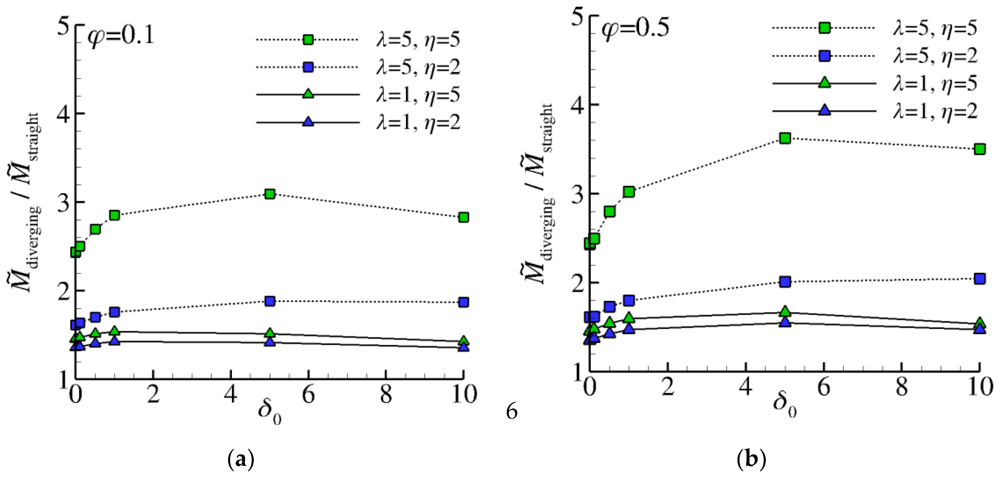
In order to reveal the quantitative differences between the straight channel flows and diverging channel flows in Figure 2, the ratio M ~ d i v e r g i n g / M ~ s t r a i g h t is plotted as a function of δ 0 , for λ = 1,5 , and η = 2,5 as well as for two values of the pressure ratio φ , namely, φ = 0.1,0.5 . The data for straight channels ( η = 1 ) were taken from [28], where an extensive database of the dimensionless mass flow for gas flows through straight channels is provided. As shown in Figure 2, under the same gas rarefaction conditions, the dimensionless mass flow rate of the diverging channel flows is higher than that of the corresponding straight channel flows. It was found that this increase in the mass flow rate in the transition regime is about 1.4–1.7 times for the case of short channels with λ = 1 and becomes even larger and about 1.6–3.6 times for the longer channels with λ = 5 .
Table 4 presents a comparison between the numerical values for the dimensionless mass flow rate M ~ obtained from the approximate kinetic approach (see Section 3.2) and those obtained from the complete 4D kinetic solution. In columns four, six, and eight of Table 4, the relative difference % of the dimensionless mass flow rates defined as
% = 100 × M ~ a p p r o x i m a t e M ~ c o m p l e t e M ~ c o m p l e t e ,
for various values of δ 0 , φ , λ , and η are reported. As can be seen, the results obtained from the approximate kinetic approach differ significantly from those obtained from the complete 4D kinetic solution. As expected, the relative difference increases as the dimensionless length λ decreases or the aspect ratio η increases. It is noted that, by either decreasing λ or increasing η , we expect the contribution of the end-effect phenomena to become more pronounced. It is also observed that the increase in the pressure ratio (decrease in pressure drop) leads to a decrease in the relative difference % , which is expected if someone considers that, in this case, the local pressure gradient decreases too. However, the relative difference % remains large in all examined values of δ 0 , φ , λ , and η , with the approximate approach always overestimating the mass flow rate values. It should be mentioned that in [24], large deviations between the complete solution and the approximate kinetic approach were reported for conical diverging flows into vacuum. A significant improvement in the description of the approximate kinetic approach is expected if someone considers the end-effect phenomena at the channel ends. The end-effect correction can be introduced into the approximate kinetic approach by elongating the length of the channel according to the local gas rarefaction conditions at the channel ends, i.e., L / H = Δ L i n l e t + L + Δ L o u t l e t / H . The correction lengths as function of the gas rarefaction parameter are available in the literature [68] in the case of gas flows through a straight channel. Given the fact that, to the best of the authors’ knowledge, the corresponding end-effect correction lengths for diverging channels are not available in the literature, the presented errors in columns five, seven, and nine of Table 4 are based on the end-effect length values for straight channels. In general, we expect further improvement in the predictions of the approximate kinetic approach after the introduction of the exact end-effect correction values for diverging channels, but this requires performing a dedicated analysis which is beyond the scope of the present study. As can be seen, by introducing the end-effect corrections of the straight channels the results of the approximate kinetic approach are improved significantly. We can conclude that in the case of diverging channel flows, the approximate kinetic approach coupled with the end-effect correction approach for straight channels can be applied to predict the mass flow rate within 15%, for small aspect ratio η = 2 and λ = 5 , as long as δ 0 < 5 , while this error drops to 10% for longer diverging channels with λ = 10 and δ 0 < 10 . Further improvement of the approximate kinetic approach is expected in the case of longer diverging channels with λ > 10 , with its validity range being extended even for larger aspect ratios η when λ 10 .
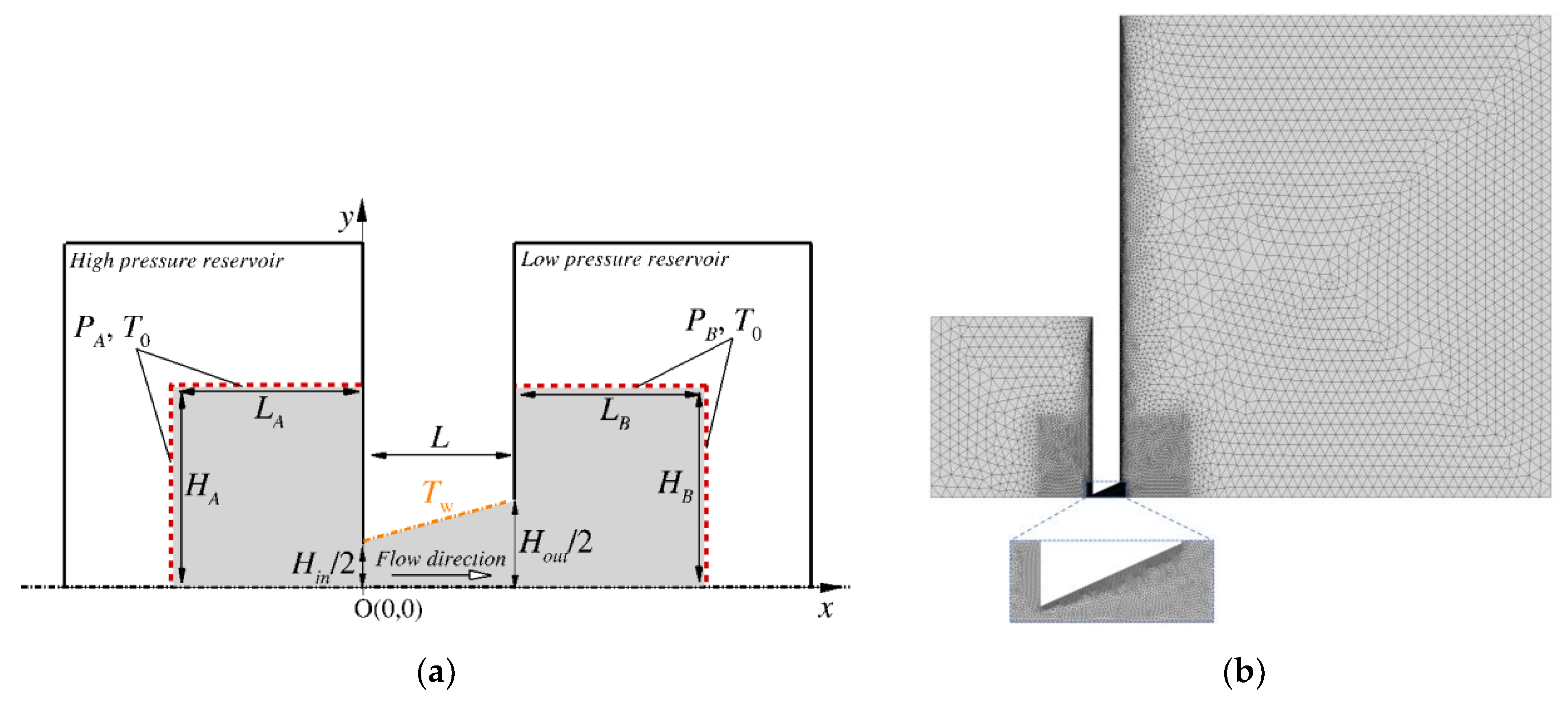
In addition to the effect of the diverging channel geometry on the mass flow rate, we are also interested in examining the corresponding effect on the distribution of macroscopic quantities of practical interest. Figure 3 illustrates the axial distributions of the dimensionless pressure P ~ , Mach number M a   = u ~ x ~ 6 / 5 T ~ , and dimensionless temperature T ~ along the symmetry axis ( y ~ = 0 ) for λ = 5 and φ = 0.5 , as well as for two indicative values of the gas rarefaction parameter δ 0 = 0.1,10 . Also, the corresponding distributions of straight channel flows ( η = 1 ) are plotted for comparison purposes. The data for the straight channel flows have been extracted from [28], where the DSMC method was applied. The reason the curves for η = 1 are not smooth is attributed to statistical noise inherent in the DSMC method. As it is seen, the axial distributions for η = 1 differ not only quantitatively but also qualitatively from that for η > 1 . With the increase in the aspect ratio η , the flow starts to obtain the characteristics of the slit flow [7,69], namely, a rapid increase in the axial velocity as the flow enters the channel followed by a rapid decrease after some distance from the channel inlet. The decrease in the pressure at the inlet of the channel becomes more rapid as the aspect ratio η increases and is enhanced significantly as the gas rarefaction level decreases (increase in δ 0 ), where the viscous effects become more important. As the flow enters the channel it is always accelerated, with this acceleration being more pronounced for divergent channels due to the weakening of the lateral wall effect on the flow. To maintain the amount of gas passing through any plane perpendicular to the line of symmetry of the channel, the velocity in the case of channels of constant cross-section increases monotonically along the channel, while in diverging channels, it slows down within the channel to balance the increase in height of the channel and the corresponding decrease in number density. A significant influence of the diverging flow geometry on the temperature profile is also observed. More specifically, a noticeable temperature drop is observed in the regions with a strong increase in velocity and, vice versa, the temperature rises with the decrease in the velocity, as a consequence of conservation of energy.
In Figure 4 and Figure 5, we extend the study of the effect of the diverging channel geometry on the distributions of macroscopic quantities, focusing on the variation in the channel length and the pressure ratio. Number density distributions are shown in Figure 4, while the corresponding axial velocity distributions are given in Figure 5. The distributions are plotted for two indicative values of λ = 1,10 and three values of φ = 0.1,0.5,0.8 , covering the cases of short and long channels, as well as the cases of large, moderate, and small pressure ratios. As can be seen in Figure 4, the behavior of the number density (and the pressure) presents the same qualitative behavior for all values of λ and φ . The effect of the aspect ratio η on the number density distributions is enhanced at larger pressure drops (smaller values of φ ), and longer channels. As observed in Figure 5, the velocity distributions for λ = 1 show qualitatively similar behavior for all examined pressure ratios. For the long channel case with λ = 10 , where the diverging geometry plays a more significant role, we observe not only quantitative differences but also significant qualitative ones among the different pressure ratios. Similarly to the short channel case with λ = 1 , for moderate and large values of φ , the flow always accelerates at the inlet, reaching its maximum value after some small distance from the inlet, and then decreases monotonically until the outlet of the channel. However, for small values of the pressure ratio φ and aspect ratio η , the flow through diverging channels maintains the well-known qualitative behavior of gas flows through straight channels, namely, the velocity increases monotonically inside the channel. This behavior is explained by the fact that for η = 2 and φ = 0.1 , the change in the number density (the number density at the outlet is 10 times less compared to the inlet) between the inlet and the outlet of the channel is larger compared to the change in the channel area (the outlet area is two times larger compared to the inlet area), while for smaller values of the pressure ratio φ , the increase in the area compensates for the change in the pressure drop. Likewise, the weaker change in the velocity inside the channel for η = 5 compared to η = 2 is explained. To obtain a better understanding of the Mach number variation inside the channel for various combinations of λ , φ , η and δ 0 , the average Mach number values at different sections of the channel are given in Table 5. The values of the Mach number remain well less than 0.3 in all examined cases for φ = 0.8 . This is indirect evidence that the compressibility effects are insignificant for this low-pressure drop. While, as the values of the Mach number indicate, they are expected to play a more significant role as the pressure drop increases with a simultaneous increase in the gas rarefaction parameter δ 0 .

4.2. Non-Isothermal Case—Effect of the Wall Temperature

In this subsection, we study the flow characteristics in the case that the wall temperature is not equal to the temperature of the gas in the reservoirs, i.e., τ 1 . The influence of the wall temperature is investigated by assuming a large temperature ratio, namely, τ = 900 / 273.15 3.3 . The reason for this choice is twofold: first, under such a large temperature difference, any potential effect of the temperature wall on the flow field is expected to be significant [27], and second, this temperature ratio covers a wide range of the examined temperature differences in [27], where the temperature wall effects were examined in the case of straight channels, allowing us to examine whether the observations made previously for the case of straight channel flows into vacuum ( φ = 0 ) also hold true for diverging channel flows. The investigation of the wall temperature effect was performed for φ = 0.1 , which can be considered as the closest one to that studied in [27]. Given the well-known inability of the hard sphere model to describe strongly non-isothermal gas flows, due to the lack of an appropriate description of the viscosity variation with temperature, the inverse power law molecular model was applied for the non-isothermal cases. This requires the definition of the viscosity index ω , with 0.5 ω 1 , which depends on the working temperature range, and is gas-specific. In the present work, the value of ω = 0.75 is considered, which corresponds to argon gas and reproduces the experimental argon viscosity data [70] within 1.5% over the entire range of the temperature variation examined here. It is noted that, this value is representative also for other gases with similar viscosity index values (e.g., Krypton) [2]. For consistency reasons, all the isothermal results presented in this subsection have been obtained using the inverse power law molecular model and the same value for ω .
In Table 6, the dimensionless mass flow rate data M ~ obtained for τ = 3.3 are compared with the corresponding isothermal ones for τ = 1 . The comparison covers a wide range of all involved parameters, namely, δ 0 , λ , and η . By comparing the data for τ = 1 in Table 6 and the corresponding hard-sphere ones in Table 3, it is clearly seen that the effect of the molecular model on M ~ in the transition regime is very weak. A similar weak dependence of the dimensionless mass flow rate on ω in the case of isothermal gas flows was reported in [5] for the case of straight channels. A strong effect of the wall temperature on M ~ is observed at high values of δ 0 . Indeed, as observed in the case of straight channels [27], the effect of the temperature wall is enhanced in low-rarefied atmospheres (large values of δ 0 ), mainly due to the fact that the higher particle collision rate makes the energy transfer mechanism more effective. For the cases close to the slip flow regime with δ 0 = 10 , the impact of τ on M ~ is increased as the aspect ratio η decreases. However, at smaller values of δ 0 , the effect of the temperature ratio becomes weaker.
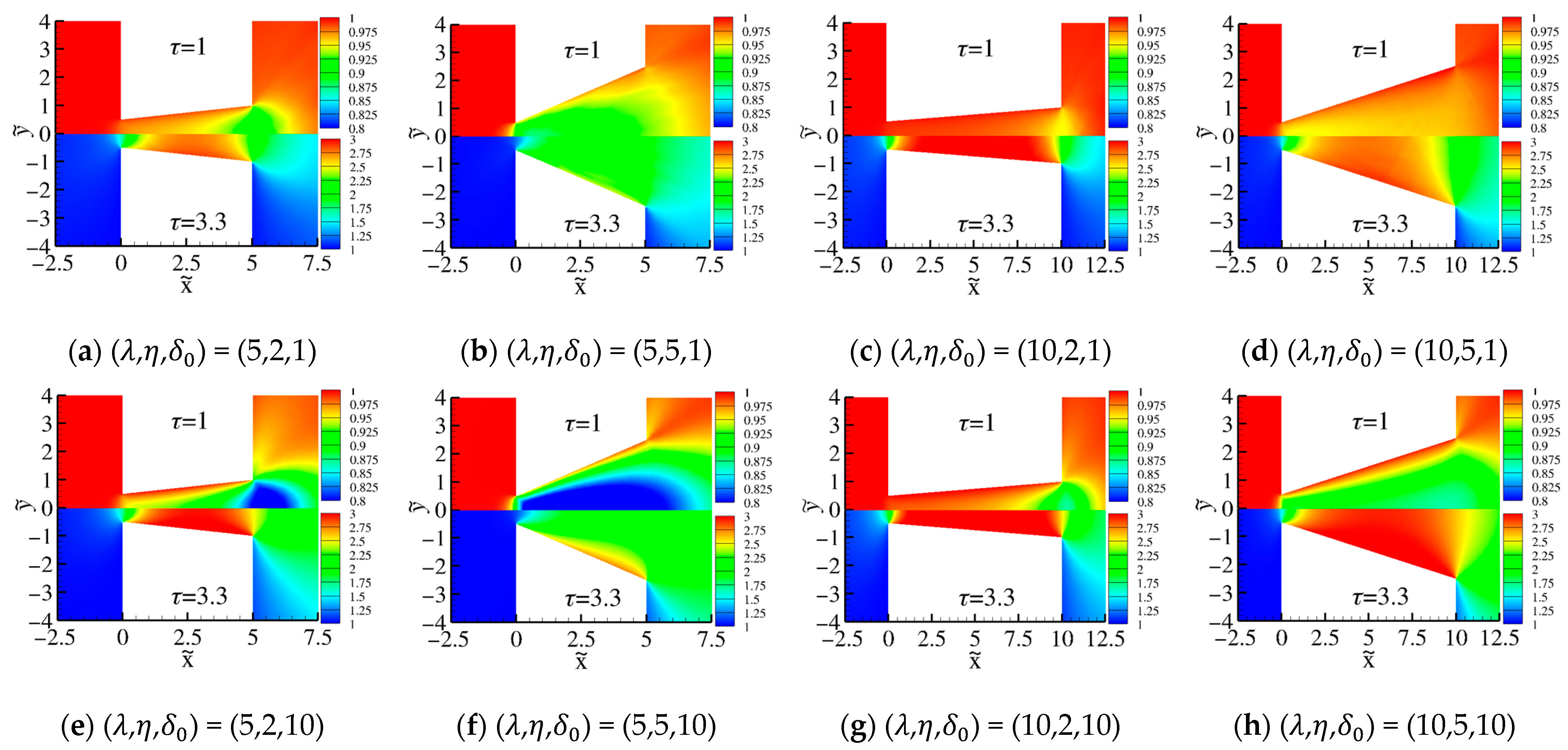
In Figure 6, the temperature contours T ~ are shown for τ = 1 and 3.3 and for δ 0 = 1,10 , η = 2,5 , and λ = 5,10 . As can be seen, the temperature wall has a strong influence on temperature contours, which also depends strongly on the geometric characteristics of the channel. It is deduced that, for τ = 3.3 , as the gas enters the channel, its dimensionless temperature increases rapidly and always remains above one (the equilibrium value in the reservoir), in contrast to the isothermal case, in which the dimensionless gas temperature is always below one. In addition, for the non-isothermal case, as the aspect ratio increases, the temperature of the gas inside the channel decreases but always remains above one. It is also evident that the increase in the gas rarefaction parameter δ 0 enhances the influence of the wall temperature, resulting in higher gas temperature values inside the channel. This can be considered as a consequence of the higher particle collision rate existing at larger values of δ 0 compared to the smaller ones, leading to an improvement in the energy transfer mechanism.
Next, in Figure 7, the corresponding pressure P ~ contours are shown. Inside the reservoirs and far away from the channel ends, the pressure remains uniform and equal to its equilibrium values. It is evident that the pressure for the non-isothermal flow case remains higher and is characterized by smoother changes compared to the isothermal flow case. In the case of τ = 1 , as the flow passes the channel, the pressure decreases monotonically, while for τ = 3.3 , this is the case only for large aspect ratios η . For smaller values of the aspect ratio ( η = 2 ), an overshoot in the pressure is observed at the entrance of the channel. The overshoot becomes more pronounced as both the channel length and the gas rarefaction increase. The overshoot is a consequence of the high inlet temperature that the gas acquires as it enters the channel in the case of non-isothermal flow and greatly exceeds the equilibrium temperature in the reservoirs. It is worthwhile mentioning that, for similar flow conditions, the overshoot in pressure was also pointed out in [27] for gas flows through straight tubes.
In Figure 8, for the same set of flow parameters as those in Figure 6 and Figure 7, the corresponding axial velocity u ~ x ~ contours are presented. The velocity contours are overlaid by the velocity streamlines. The velocity contours under isothermal and non-isothermal conditions present the same qualitative picture. However, the velocity increases noticeably as the wall temperature increases too. The streamlines do not align with the x ~ -axis, highlighting the 2D character of the gas velocity. This may partially explain the deviations mentioned in Table 4 between the complete kinetic solution and the approximate kinetic solution. The approximate kinetic solution requires the velocity to be one-directional (in the x ~ -direction) at each cross-section, and the flow is pure isothermal.

5. Conclusions

In the present work, the flow through diverging channels is studied parametrically, covering a wide range of geometry and flow parameters. The analysis is performed considering the complete flow domain, including the upstream and downstream reservoirs, without introducing computational domain simplifications by applying artificial boundary conditions at the inlet and at the outlet of the channel. The kinetic solution is based on the Shakhov kinetic model assuming diffuse boundary conditions on the solid walls. Two different molecular models have been applied, namely, the hard-sphere model and the inverse power law model. The applied deterministic approach allowed us to perform the present analysis in a wide range of pressure ratios, including the case of small pressure drops, which have not yet been studied thoroughly.
The main findings can be summarized as follows:
  • The effect of the geometry parameters, namely dimensionless length λ and the aspect ratio η on M ~ , remains quantitatively significant over the entire range of the pressure ratio φ .
  • The values of the dimensionless mass flow rates in the diverging channel flows are significantly higher compared to the corresponding ones in the straight channel flows, not only for large pressure drops but also for small pressure drops. For channels with λ > 1 and φ 0.1 , at least an increase between 1.5 and 3 times can be expected in the transition flow regime.
  • This study confirms the existence of a shallow Knudsen minimum for all values of the pressure ratio φ in the case of long channels ( λ = 10 ) with small values of the aspect ratio η = 2 . No Knudsen minimum is observed for η = 5 , even for the longest examined channel case with λ = 10 .
  • Attention should be paid to the use of the approximate kinetic approach (Section 3.2), which makes use of the fully developed flow data when flows through diverging channels are considered. Although the accuracy of the approximate kinetic approach improves as the pressure drop decreases, the deviations compared to the complete flow solution (Section 3.1) remain high even for relatively long channels with λ = 10 . However, the present analysis shows that by applying the end-effect correction lengths of the straight channel flow, the validity range of the approximate kinetic approach is improved significantly. More specifically, the application of the approximate kinetic approach coupled with the end-effect correction approach results in a maximum deviation of less than 10% when λ 10 and η 2 .
  • The diverging channel geometry has a significant effect on the distributions of the macroscopic quantities. The analysis shows that an increase in the aspect ratio of the channel η causes a drop of the pressure (and density) in the channel not only for flows under large pressure drops but also for small ones. In addition, depending on the pressure ratio, the velocity distributions may differ, not only quantitatively but also qualitatively, compared to the corresponding ones reported in the literature for straight channel flows.
  • The influence of the wall temperature on the mass flow rate is observed to be strong in less-rarefied cases, with the mass flow rate being a decreasing function of the temperature ratio τ , while this influence is reduced as the channel aspect ratio η increases. In the highly rarefied cases, the influence was noticeably smaller.
Overall, the present analysis is expected to be useful in the development and optimization of technological devices in vacuum and aerospace technologies. The provided data can also be used as a reference point for testing other numerical approaches and kinetic models. It is noted that the applied diffuse gas–surface interaction is a reliable model for noble gases with sufficiently large gas molecular mass and typically technical surfaces. However, for light gases such as helium and for atomically clean surfaces, a more advanced type of gas–surface interaction should be applied. Thus, in the future, this work may be extended by considering more advanced types of gas–surface interactions. In addition, this study can be further extended by considering also polyatomic gases in order to investigate any possible effects related to the internal degrees of freedom of the polyatomic gas molecules. Given the expected increase in the computational cost by adding more physical complexity to the modeling, a possible further acceleration of the simulation of the current flow set-up may be achieved by the use of the general synthetic iterative scheme (GSIS) [71].

Author Contributions

Conceptualization: C.T. and F.L.; methodology: C.T., F.L. and T.T.; software: C.T., F.L. and T.T.; validation: C.T., F.L. and T.T.; formal analysis: C.T., F.L., and T.T.; investigation: C.T., F.L., T.T., I.S. and C.D.; resources: C.D.; data curation: C.T. and F.L.; writing—original draft preparation: C.T., F.L., T.T., I.S. and C.D.; writing—review and editing: C.T., F.L., T.T., I.S. and C.D.; visualization: C.T., F.L. and T.T.; supervision: C.T. and C.D.; project administration: C.T. and I.S. All authors have read and agreed to the published version of the manuscript.

Funding

This research received no external funding.

Data Availability Statement

The data that supports the findings of this study are available within this article. Additional data may be made available upon reasonable request from the corresponding author.

Acknowledgments

The authors would like to thank Stylianos Varoutis for providing the DSMC data for the straight channels used in Figure 3.

Conflicts of Interest

The authors declare no conflict of interest.

References

  1. Cercignani, C. The Boltzmann Equation: Some Mathematical Aspects. In Kinetic Theory and Gas Dynamics; Cercignani, C., Ed.; International Centre for Mechanical Sciences; Springer: Vienna, Austria, 1988; pp. 1–36. ISBN 978-3-7091-2762-9. [Google Scholar]
  2. Bird, G.A. Molecular Gas Dynamics and the Direct Simulation of Gas Flows; Oxford Engineering Science Series; Clarendon Press: Oxford, UK; Oxford University Press: Oxford, NY, USA, 1994; ISBN 978-0-19-856195-8. [Google Scholar]
  3. Sharipov, F. Rarefied Gas Dynamics: Fundamentals for Research and Practice; Wiley-VCH Verlag GmbH & Co. KGaA: Weinheim, Germany, 2016; ISBN 978-3-527-68553-0. [Google Scholar]
  4. Varoutis, S.; Hauer, V.; Day, C.; Pantazis, S.; Valougeorgis, D. Experimental and Numerical Investigation in Flow Configurations Related to the Vacuum Systems of Fusion Reactors. Fusion Eng. Des. 2010, 85, 1798–1802. [Google Scholar] [CrossRef]
  5. Varoutis, S.; Valougeorgis, D.; Sazhin, O.; Sharipov, F. Rarefied Gas Flow through Short Tubes into Vacuum. J. Vac. Sci. Technol. A 2008, 26, 228–238. [Google Scholar] [CrossRef]
  6. Sharipov, F.; Kozak, D.V. Rarefied Gas Flow through a Thin Slit into Vacuum Simulated by the Monte Carlo Method over the Whole Range of the Knudsen Number. J. Vac. Sci. Technol. Vac. Surf. Films 2009, 27, 479–484. [Google Scholar] [CrossRef]
  7. Graur, I.; Polikarpov, A.P.; Sharipov, F. Numerical Modeling of Rarefied Gas Flow through a Slit into Vacuum Based on the Kinetic Equation. Comput. Fluids 2011, 49, 87–92. [Google Scholar] [CrossRef]
  8. Sharipov, F.; Seleznev, V. Data on Internal Rarefied Gas Flows. J. Phys. Chem. Ref. Data 1998, 27, 657–706. [Google Scholar] [CrossRef]
  9. Graur, I.; Sharipov, F. Gas Flow through an Elliptical Tube over the Whole Range of the Gas Rarefaction. Eur. J. Mech.-B/Fluids 2008, 27, 335–345. [Google Scholar] [CrossRef]
  10. Breyiannis, G.; Varoutis, S.; Valougeorgis, D. Rarefied Gas Flow in Concentric Annular Tube: Estimation of the Poiseuille Number and the Exact Hydraulic Diameter. Eur. J. Mech.-B/Fluids 2008, 27, 609–622. [Google Scholar] [CrossRef]
  11. Varoutis, S.; Naris, S.; Hauer, V.; Day, C.; Valougeorgis, D. Computational and Experimental Study of Gas Flows through Long Channels of Various Cross Sections in the Whole Range of the Knudsen Number. J. Vac. Sci. Technol. Vac. Surf. Films 2009, 27, 89–100. [Google Scholar] [CrossRef]
  12. Cervone, A.; Mancas, A.; Zandbergen, B. Conceptual Design of a Low-Pressure Micro-Resistojet Based on a Sublimating Solid Propellant. Acta Acta Astronaut. 2015, 108, 30–39. [Google Scholar] [CrossRef]
  13. Alexeenko, A.A.; Fedosov, D.A.; Gimelshein, S.F.; Levin, D.A.; Collins, R.J. Transient Heat Transfer and Gas Flow in a MEMS-Based Thruster. J. Microelectromech. Syst. 2006, 15, 181–194. [Google Scholar] [CrossRef]
  14. Markelov, G.N. Numerical Study of 2D/3D Micronozzle Flows. AIP Conf. Proc. 2001, 585, 539–546. [Google Scholar] [CrossRef]
  15. Zuppardi, G.; Esposito, A. Aerodynamic Characterization of the Jet of an Arc Wind Tunnel. AIP Conf. Proc. 2016, 1786, 190003. [Google Scholar] [CrossRef]
  16. Tatsios, G.; Lopez Quesada, G.; Rojas-Cardenas, M.; Baldas, L.; Colin, S.; Valougeorgis, D. Computational Investigation and Parametrization of the Pumping Effect in Temperature-Driven Flows through Long Tapered Channels. Microfluid. Nanofluid. 2017, 21, 99. [Google Scholar] [CrossRef]
  17. Wang, X.; Su, T.; Zhang, W.; Zhang, Z.; Zhang, S. Knudsen Pumps: A Review. Microsyst. Nanoeng. 2020, 6, 26. [Google Scholar] [CrossRef] [PubMed]
  18. Sazhin, O.; Sazhin, A. Rarefied Gas Flow into Vacuum through Linearly Diverging and Converging Channels. Int. J. Heat Mass Transf. 2023, 203, 123842. [Google Scholar] [CrossRef]
  19. Darbandi, M.; Roohi, E. Study of Subsonic–Supersonic Gas Flow through Micro/Nanoscale Nozzles Using Unstructured DSMC Solver. Microfluid. Nanofluid. 2011, 10, 321–335. [Google Scholar] [CrossRef]
  20. Saadati, S.A.; Roohi, E. Detailed Investigation of Flow and Thermal Field in Micro/Nano Nozzles Using Simplified Bernoulli Trial (SBT) Collision Scheme in DSMC. Aerosp. Sci. Technol. 2015, 46, 236–255. [Google Scholar] [CrossRef]
  21. Ebrahimi, A.; Roohi, E. DSMC Investigation of Rarefied Gas Flow through Diverging Micro- and Nanochannels. Microfluid. Nanofluid. 2017, 21, 18. [Google Scholar] [CrossRef]
  22. Ebrahimi, A.; Shahabi, V.; Roohi, E. Pressure-Driven Nitrogen Flow in Divergent Microchannels with Isothermal Walls. Appl. Sci. 2021, 11, 3602. [Google Scholar] [CrossRef]
  23. Tatsios, G.; Valougeorgis, D.; Stefanov, S.K. Reconsideration of the Implicit Boundary Conditions in Pressure Driven Rarefied Gas Flows through Capillaries. Vacuum 2019, 160, 114–122. [Google Scholar] [CrossRef]
  24. Titarev, V.A.; Shakhov, E.M.; Utyuzhnikov, S.V. Rarefied Gas Flow through a Diverging Conical Pipe into Vacuum. Vacuum 2014, 101, 10–17. [Google Scholar] [CrossRef]
  25. Yakunchikov, A.; Kosyanchuk, V. Application of Event-Driven Molecular Dynamics Approach to Rarefied Gas Dynamics Problems. Comput. Fluids 2018, 170, 121–127. [Google Scholar] [CrossRef]
  26. Graur, I.; Ho, M.T. Rarefied Gas Flow through a Long Rectangular Channel of Variable Cross Section. Vacuum 2014, 101, 328–332. [Google Scholar] [CrossRef]
  27. Zhang, M.; Day, C.; Varoutis, S.; Cai, G. Rarefied Gas Flow into Vacuum through Short Tubes at Variable Wall Temperatures. J. Vac. Sci. Technol. A 2017, 35, 021604. [Google Scholar] [CrossRef]
  28. Varoutis, S.; Day, C.; Sharipov, F. Rarefied Gas Flow through Channels of Finite Length at Various Pressure Ratios. Vacuum 2012, 86, 1952–1959. [Google Scholar] [CrossRef]
  29. Shakhov, E.M. Generalization of the Krook Kinetic Relaxation Equation. Fluid Dyn. 1968, 3, 95–96. [Google Scholar] [CrossRef]
  30. Titarev, V.A.; Shakhov, E.M. Kinetic Analysis of the Isothermal Flow in a Long Rectangular Microchannel. Comput. Math. Math. Phys. 2010, 50, 1221–1237. [Google Scholar] [CrossRef]
  31. Polikarpov, A.P.; Graur, I. Unsteady Rarefied Gas Flow through a Slit. Vacuum 2014, 101, 79–85. [Google Scholar] [CrossRef]
  32. Pan, D.; Zhong, C.; Zhuo, C. An Implicit Discrete Unified Gas-Kinetic Scheme for Simulations of Steady Flow in All Flow Regimes. Commun. Comput. Phys. 2019, 25, 1469–1495. [Google Scholar] [CrossRef]
  33. Tantos, C.; Teichmann, T.; Sarris, I.; Day, C. Extensive Analysis of the Applicability Range of the Linear Kinetic Approaches in the Case of the Pressure Driven Gas Mixture Flows. Phys. Fluids 2024, 36, 012009. [Google Scholar] [CrossRef]
  34. Sharipov, F. Rarefied Gas Flow through a Long Tube at Any Temperature Ratio. J. Vac. Sci. Technol. A 1996, 14, 2627–2635. [Google Scholar] [CrossRef]
  35. Sharipov, F. Non-Isothermal Rarefied Gas Flow through a Slit. Phys. Fluids 1997, 9, 1804–1810. [Google Scholar] [CrossRef]
  36. Titarev, V.A.; Shakhov, E.M. Nonisothermal Gas Flow in a Long Channel Analyzed on the Basis of the Kinetic S-Model. Comput. Math. Math. Phys. 2010, 50, 2131–2144. [Google Scholar] [CrossRef]
  37. Titarev, V.A.; Shakhov, E.M. Efficient Method for Computing Rarefied Gas Flow in a Long Finite Plane Channel. Comput. Math. Math. Phys. 2012, 52, 269–284. [Google Scholar] [CrossRef]
  38. Pantazis, S.; Naris, S.; Tantos, C.; Valougeorgis, D.; André, J.; Millet, F.; Perin, J.P. Nonlinear Vacuum Gas Flow through a Short Tube Due to Pressure and Temperature Gradients. Fusion Eng. Des. 2013, 88, 2384–2387. [Google Scholar] [CrossRef]
  39. Titarev, V.A.; Shakhov, E.M.; Frolova, A.A. Shock Wave Reflection from a Short Orifice Open to Vacuum. Vacuum 2019, 161, 232–241. [Google Scholar] [CrossRef]
  40. Zhu, L.; Guo, Z. Application of Discrete Unified Gas Kinetic Scheme to Thermally Induced Nonequilibrium Flows. Comput. Fluids 2019, 193, 103613. [Google Scholar] [CrossRef]
  41. Tantos, C. Polyatomic Thermal Creep Flows through Long Microchannels at Large Temperature Ratios. J. Vac. Sci. Technol. A 2019, 37, 051602. [Google Scholar] [CrossRef]
  42. Rojas-Cárdenas, M.; Graur, I.; Perrier, P.; Méolans, J.G. Time-Dependent Experimental Analysis of a Thermal Transpiration Rarefied Gas Flow. Phys. Fluids 2013, 25, 072001. [Google Scholar] [CrossRef]
  43. Sharipov, F.; Bertoldo, G. Heat Transfer through a Rarefied Gas Confined between Two Coaxial Cylinders with High Radius Ratio. J. Vac. Sci. Technol. A 2006, 24, 2087–2093. [Google Scholar] [CrossRef]
  44. Li, Z.-H.; Zhang, H.-X. Gas-Kinetic Description of Shock Wave Structures by Solving Boltzmann Model Equation. Int. J. Comput. Fluid Dyn. 2008, 22, 623–638. [Google Scholar] [CrossRef]
  45. Khan, M.A.; Jobic, Y.; Graur, I.; Hadj-Nacer, M.; Zampella, C.; Greiner, M. Experimentally-Benchmarked Kinetic Simulations of Heat Transfer through Rarefied Gas with Constant Heat Flux at the Boundary. Int. J. Heat Mass Transf. 2021, 176, 121378. [Google Scholar] [CrossRef]
  46. Bond, D.M.; Macrossan, M.N.; Wheatley, V. Comparison of Discrete BGK-Shakhov System with DSMC. AIP Conf. Proc. 2012, 1501, 350–357. [Google Scholar] [CrossRef]
  47. Aristov, V.V.; Shakhov, E.M.; Titarev, V.A.; Zabelok, S.A. Comparative Study for Rarefied Gas Flow into Vacuum through a Short Circular Pipe. Vacuum 2014, 103, 5–8. [Google Scholar] [CrossRef]
  48. Tatsios, G.; Vargas, M.H.; Stefanov, S.K.; Valougeorgis, D. Nonequilibrium Gas Flow and Heat Transfer in a Heated Square Microcavity. Heat Transf. Eng. 2016, 37, 1085–1095. [Google Scholar] [CrossRef]
  49. Titarev, V.A.; Frolova, A.A.; Rykov, V.A.; Vashchenkov, P.V.; Shevyrin, A.A.; Bondar, Y.A. Comparison of the Shakhov Kinetic Equation and DSMC Method as Applied to Space Vehicle Aerothermodynamics. J. Comput. Appl. Math. 2020, 364, 112354. [Google Scholar] [CrossRef]
  50. Misdanitis, S.; Pantazis, S.; Valougeorgis, D. Pressure Driven Rarefied Gas Flow through a Slit and an Orifice. Vacuum 2012, 86, 1701–1708. [Google Scholar] [CrossRef]
  51. Tantos, C.; Varoutis, S.; Day, C. Deterministic and Stochastic Modeling of Rarefied Gas Flows in Fusion Particle Exhaust Systems. J. Vac. Sci. Technol. B 2020, 38, 064201. [Google Scholar] [CrossRef]
  52. Tantos, C.; Valougeorgis, D. Conductive Heat Transfer in Rarefied Binary Gas Mixtures Confined between Parallel Plates Based on Kinetic Modeling. Int. J. Heat Mass Transf. 2018, 117, 846–860. [Google Scholar] [CrossRef]
  53. Tantos, C. Steady Planar Couette Flow of Rarefied Binary Gaseous Mixture Based on Kinetic Modeling. Eur. J. Mech.-B/Fluids 2019, 76, 375–389. [Google Scholar] [CrossRef]
  54. Yang, W.; Gu, X.-J.; Emerson, D.R.; Zhang, Y.; Tang, S. Modelling Thermally Induced Non-Equilibrium Gas Flows by Coupling Kinetic and Extended Thermodynamic Methods. Entropy 2019, 21, 816. [Google Scholar] [CrossRef]
  55. Ho, M.T.; Li, J.; Wu, L.; Reese, J.M.; Zhang, Y. A Comparative Study of the DSBGK and DVM Methods for Low-Speed Rarefied Gas Flows. Comput. Fluids 2019, 181, 143–159. [Google Scholar] [CrossRef]
  56. Li, J. Simulation Methods for Rarefied Gas Flows. In Multiscale and Multiphysics Flow Simulations of Using the Boltzmann Equation: Applications to Porous Media and MEMS; Li, J., Ed.; Springer International Publishing: Cham, Switzerland, 2020; pp. 67–117. ISBN 978-3-030-26466-6. [Google Scholar]
  57. Liu, Z.J.; Shu, C.; Chen, S.Y.; Yang, L.M.; Wan, M.P.; Liu, W. A Novel Solver for Simulation of Flows from Continuum Regime to Rarefied Regime at Moderate Knudsen Number. J. Comput. Phys. 2020, 415, 109548. [Google Scholar] [CrossRef]
  58. Polikarpov, A.; Graur, I.; Sharipov, F. Sublimation and Deposition in Gaseous Mixtures. Int. J. Heat Mass Transf. 2020, 160, 120213. [Google Scholar] [CrossRef]
  59. Voronich, I.V.; Titarev, V.A. Numerical Analysis of Rarefied Gas Flow through a System of Short Channels. Comput. Math. Math. Phys. 2023, 63, 2227–2243. [Google Scholar] [CrossRef]
  60. Basdanis, T.; Valougeorgis, D.; Sharipov, F. Viscous and Thermal Velocity Slip Coefficients via the Linearized Boltzmann Equation with Ab Initio Potential. Microfluid. Nanofluid. 2023, 27, 75. [Google Scholar] [CrossRef]
  61. Guo, Z.; Xu, K.; Wang, R. Discrete Unified Gas Kinetic Scheme for All Knudsen Number Flows: Low-Speed Isothermal Case. Phys. Rev. E 2013, 88, 033305. [Google Scholar] [CrossRef] [PubMed]
  62. Guo, Z.; Wang, R.; Xu, K. Discrete Unified Gas Kinetic Scheme for All Knudsen Number Flows. II. Thermal Compressible Case. Phys. Rev. E 2015, 91, 033313. [Google Scholar] [CrossRef] [PubMed]
  63. Zhang, Y.; Zhu, L.; Wang, R.; Guo, Z. Discrete Unified Gas Kinetic Scheme for All Knudsen Number Flows. III. Binary Gas Mixtures of Maxwell Molecules. Phys. Rev. E 2018, 97, 053306. [Google Scholar] [CrossRef] [PubMed]
  64. SALOME PLATFORM-The Open-Source Platform for Numerical Simulation. Available online: https://www.salome-platform.org/ (accessed on 17 January 2024).
  65. Sharipov, F. Rarefied Gas Flow through a Long Tube at Arbitrary Pressure and Temperature Drops. J. Vac. Sci. Technol. A 1997, 15, 2434–2436. [Google Scholar] [CrossRef]
  66. Sharipov, F.; Bertoldo, G. Rarefied Gas Flow through a Long Tube of Variable Radius. J. Vac. Sci. Technol. A 2005, 23, 531–533. [Google Scholar] [CrossRef]
  67. Tantos, C.; Kritikos, E.; Varoutis, S.; Day, C. Kinetic Modeling of Polyatomic Heat and Mass Transfer in Rectangular Microchannels. Heat Mass Transf. 2023, 59, 167–184. [Google Scholar] [CrossRef]
  68. Pantazis, S.; Valougeorgis, D.; Sharipov, F. End Corrections for Rarefied Gas Flows through Capillaries of Finite Length. Vacuum 2013, 97, 26–29. [Google Scholar] [CrossRef]
  69. Graur, I.A.; Polikarpov, A.P.; Sharipov, F. Numerical Modelling of Rarefied Gas Flow through a Slit at Arbitrary Pressure Ratio Based on the Kinetic Equation. Z. Angew. Math. Phys. 2012, 63, 503–520. [Google Scholar] [CrossRef]
  70. Kestin, J.; Knierim, K.; Mason, E.A.; Najafi, B.; Ro, S.T.; Waldman, M. Equilibrium and Transport Properties of the Noble Gases and Their Mixtures at Low Density. J. Phys. Chem. Ref. Data 1984, 13, 229–303. [Google Scholar] [CrossRef]
  71. Liu, W.; Zhang, Y.; Zeng, J.; Wu, L. Further Acceleration of Multiscale Simulation of Rarefied Gas Flow via a Generalized Boundary Treatment. J. Comput. Phys. 2024, 503, 112830. [Google Scholar] [CrossRef]
Figure 1. (a) Schematic diagram of the examined flow configuration; (b) illustrative example of the numerical grid used in the simulations in the case of λ = 5 and η = 5.
Fluids 09 00078 g001
Figure 2. Ratio of the dimensionless mass flow rates M ~ d i v e r g i n g / M ~ s t r a i g h t vs. δ 0 , for λ = 1,5 , η = 2,5 and two indicative pressure ratios, namely, (a) φ = 0.1 ; and (b) φ = 0.5 .
Fluids 09 00078 g002
Figure 3. Distributions of the dimensionless pressure P ~ (a), Mach number M a (b), and dimensionless temperature T ~ (c) along the symmetry axis ( y ~ = 0 ) for δ 0 = 0.1,10 , λ = 5 , η = 1,2 , 5 , and φ = 0.5 . The data for δ 0 = 0.1 and 10 are shown with the dashed and solid lines, respectively.
Fluids 09 00078 g003
Figure 4. Distributions of the dimensionless number density n ~ along the symmetry axis ( y ~ = 0 ) for η = 2,5 , φ = 0.1,0.5,0.8 , at δ 0 = 1 (a,b) and 10 (c,d), with λ = 1 (a,c) and 10 (b,d). The data for η = 2 and 5 are shown with the dashed and solid lines, respectively.
Fluids 09 00078 g004
Figure 5. Distributions of the dimensionless longitudinal velocity component u ~ x ~ along the symmetry axis ( y ~ = 0 ) for η = 2,5 , φ = 0.1,0.5,0.8 , at δ 0 = 1 (a,b) and 10 (c,d), with λ = 1 (a,c) and 10 (b,d). The data for η = 2 and 5 are shown with the dashed and solid lines, respectively.
Fluids 09 00078 g005
Figure 6. Contours of the dimensionless temperature T ~ for τ = [1,3.3], δ0 = [1,10], and λ = [5,10]. In each subfigure, the upper part shows the results for τ = 1, and the lower part shows the results for τ = 3.3.
Fluids 09 00078 g006
Figure 7. Contours of the dimensionless pressure P ~ for τ = [1,3.3], δ0 = [1,10], and λ = [5,10]. In each subfigure, the upper part shows the results for τ = 1, and the lower part for τ = 3.3.
Fluids 09 00078 g007
Figure 8. Contours of the dimensionless axial velocity u ~ x ~ for τ = [1,3.3], δ0 = [1,10], and λ = [5,10]. In each subfigure, the upper part shows the results for τ = 1, and the lower part for τ = 3.3.
Fluids 09 00078 g008
Table 1. Comparison between the dimensionless mass flow rate M ~ obtained in the present work and the corresponding DSMC ones for straight channels ( η = 1 ) in [28] and for diverging channels ( η = 2 ) in [18], with λ = 1 and for various values of δ 0 and φ . Inside the parentheses the absolute percentage error is shown.
δ 0 φ
0.1   ( η = 1 ) 0.5   ( η = 1 ) 0   ( η = 2 )
[28]Present Work[28]Present Work[18]Present Work
0.10.6300.630 (0.0%)0.3540.354 (0.0%)0.9510.946 (0.53%)
10.7060.716 (1.4%)0.4190.428 (2.1%)1.061.04 (0.94%)
101.031.02 (0.97%)0.8320.838 (0.72%)1.391.39 (0.0%)
Table 2. Comparison between our mass flow rate data M ~ λ / π using the approximate kinetic approach and the corresponding ones in [26] based on the same approach for various values of δ 0 and φ with η = 10 and τ = 1 . Inside the parentheses, the absolute percentage error is shown.
φ δ 0 [26]Present Work
0.10.118.318.4 (0.55%)
113.914.0 (0.72%)
1025.025.0 (0.0%)
0.50.19.459.52 (0.74%)
17.957.98 (0.38%)
1017.417.4 (0.0%)
0.90.11.821.84 (1.10%)
11.661.66 (0.0%)
104.144.15 (0.24%)
Table 3. Mass flow rate data M ~ based on the complete 4D kinetic solution for various values of δ 0 , φ , λ , and η with τ = 1 .
λ η δ 0 φ
0.10.50.8
1200.8370.4650.186
0.10.8620.486 0.196
0.50.9360.551 0.227
11.000.617 0.260
51.280.983 0.470
101.401.23 0.685
500.8980.499 0.199
0.10.9270.523 0.211
0.51.010.595 0.246
11.080.668 0.282
51.361.06 0.519
101.471.280.748
5200.5170.287 0.115
0.10.5250.293 0.118
0.50.5480.313 0.127
10.571 0.3350.138
50.733 0.4970.220
100.893 0.680 0.322
500.7800.433 0.174
0.10.802 0.4520.182
0.50.867 0.507 0.208
10.928 0.562 0.235
51.20 0.8960.419
101.351.160.619
10200.3640.2030.0812
0.10.3630.2010.0803
0.50.3610.2020.0812
10.3660.2090.0850
50.4550.2950.129
100.5780.4090.187
500.6230.3460.139
0.10.6360.3560.143
0.50.6700.3830.156
10.7050.4150.172
50.9320.6500.294
101.130.8940.439
Table 4. Relative difference % in the dimensionless mass flow rates between the complete 4D kinetic solution and the approximate kinetic approach for various values of δ 0 , φ , λ , and η with (w/) and without (w/o) including end-effects correction lengths.
λ η δ 0 φ
0.10.50.8
w/ow/ w/ow/ w/ow/
120.54846.0841932.139534.5
140720.734744.132543.4
535167.926259.422748.1
1043312430290.222352.9
50.5119919110792411037245
11049227941267906272
51027366839329746286
1013245501023432776315
520.51005.0482.915.377.415.4
178.38.7364.615.960.515.2
557.117.543.114.239.612.4
1066.830.644.918.537.312.3
50.520278.517785.516984.1
116878.514780.914180.0
515599.012279.211069.2
1021015014710211173.0
1020.551.44.3341.69.4938.89.43
139.25.4731.99.0130.08.63
526.48.1920.77.0819.56.58
1028.713.120.48.3318.16.32
50.595.645.283.046.879.345.8
176.641.167.441.565.241.1
564.944.452.936.649.233.3
1085.565.860.944.849.134.2
Table 5. Average Mach number at the inlet, middle, and outlet of the channel for various values of δ 0 , φ , λ , and η .
λ η δ 0 φ
0.10.50.8
InletMiddle OutletInletMiddle OutletInletMiddle Outlet
120.10.450.510.530.190.160.130.0650.0470.036
10.500.600.630.240.200.160.0860.0630.048
100.660.911.10.510.470.380.230.170.13
50.10.540.400.310.210.0910.0590.0700.0260.016
10.610.490.390.270.120.0770.0940.0350.021
100.760.810.740.560.270.160.260.100.058
1020.10.130.190.340.0660.0630.0570.0250.0190.015
10.130.190.350.0680.0650.0610.0260.0200.016
100.190.270.600.130.130.120.0580.0450.036
50.10.270.290.270.130.0640.0420.0460.0180.011
10.280.310.310.150.0760.0500.0550.0210.013
100.450.540.600.320.170.110.140.0560.034
Table 6. Mass flow rate data M ~ based on the complete 4D kinetic solution for various values of δ 0 , λ , and η with τ = 3.3 and τ = 1 , in the case of ω = 0.75.
λ η δ 0 φ
13.3
520.10.5250.517
10.5710.500
100.8940.484
50.10.8020.799
10.9280.878
101.351.06
1020.10.3630.356
10.3660.313
100.5790.272
50.10.6360.631
10.7050.635
101.130.660
Disclaimer/Publisher’s Note: The statements, opinions and data contained in all publications are solely those of the individual author(s) and contributor(s) and not of MDPI and/or the editor(s). MDPI and/or the editor(s) disclaim responsibility for any injury to people or property resulting from any ideas, methods, instructions or products referred to in the content.

