
Complex-Geometry 3D Computational Fluid Dynamics with Automatic Load Balancing
 , ,
, ,
Abstract
:1. Motivation and Significance
- The software implementation in Xyst enables the exploitation of the advanced features of the Charm++ runtime system with a fluid solver;
- The implementation is public and open source.
2. Software Description
2.1. The Equations of Compressible Flow
2.2. The Numerical Method
3. Illustrative Examples
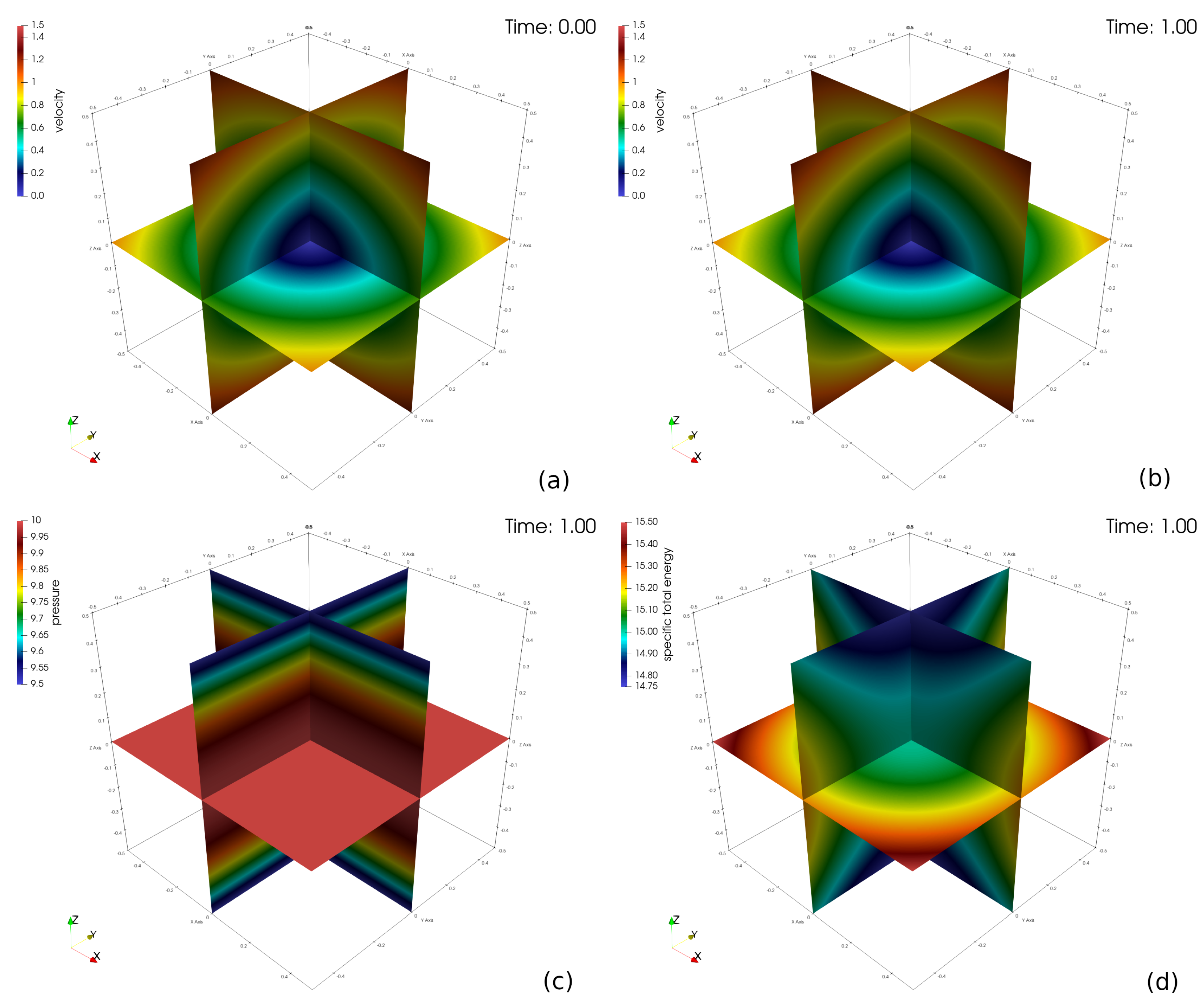
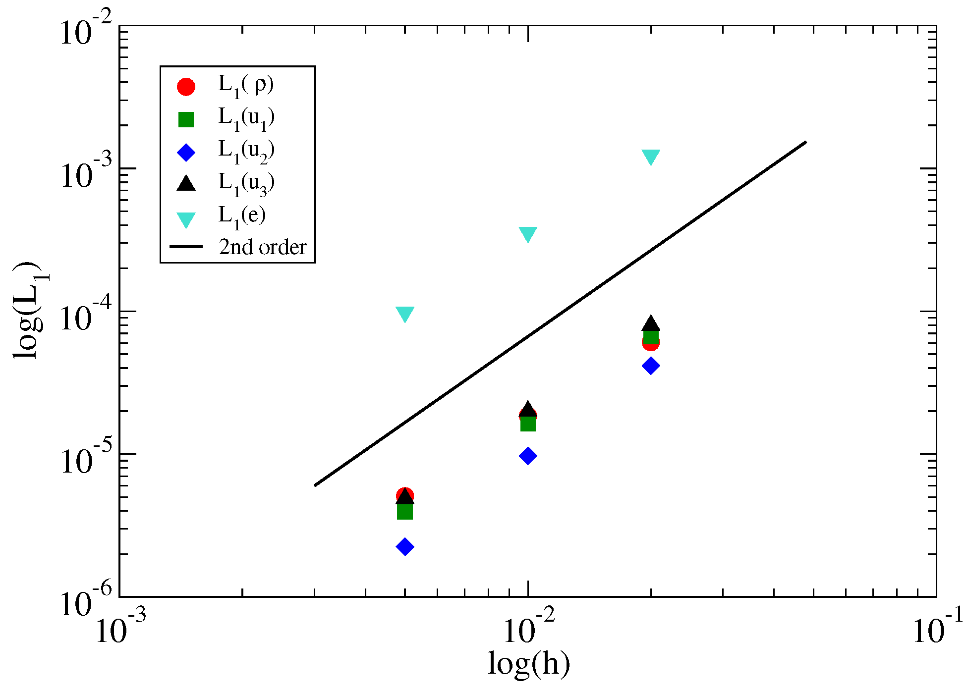
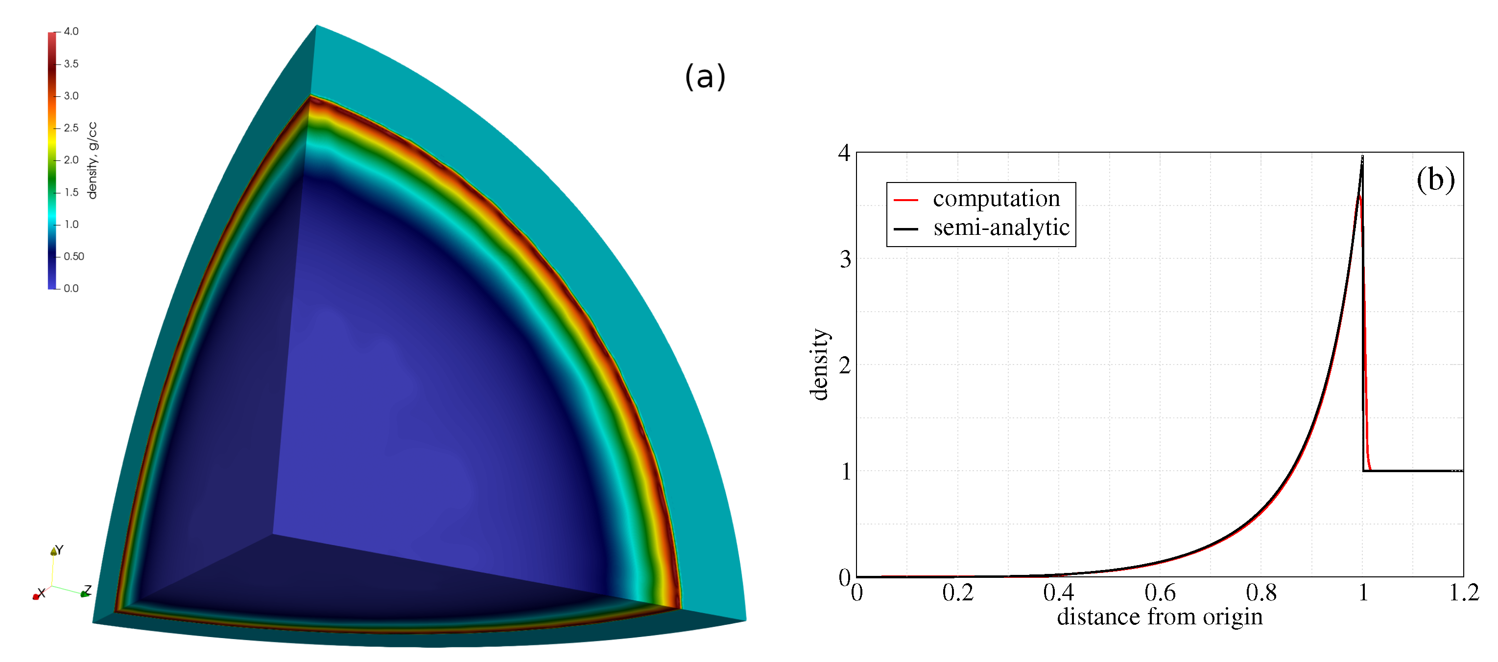
3.1. Verification
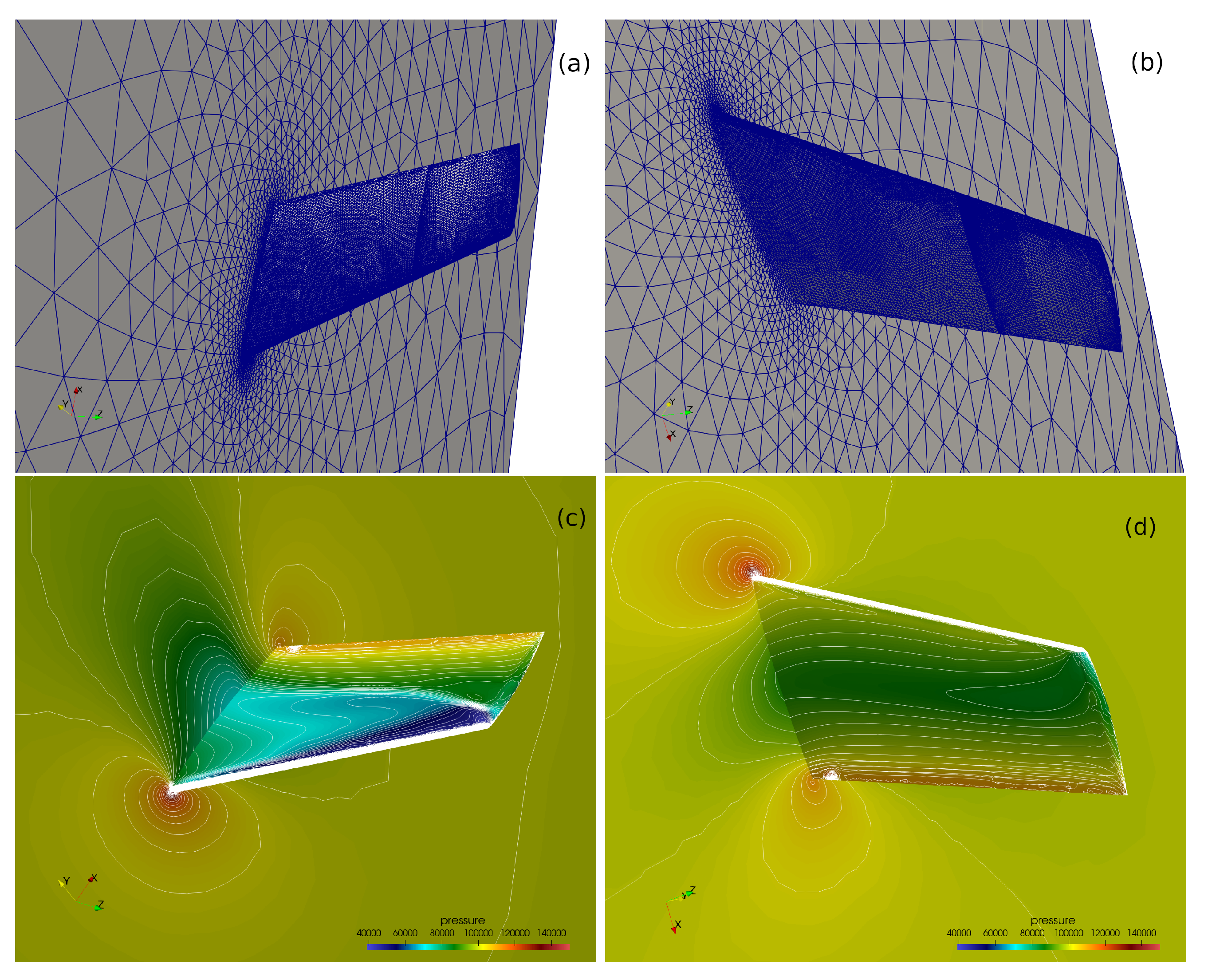
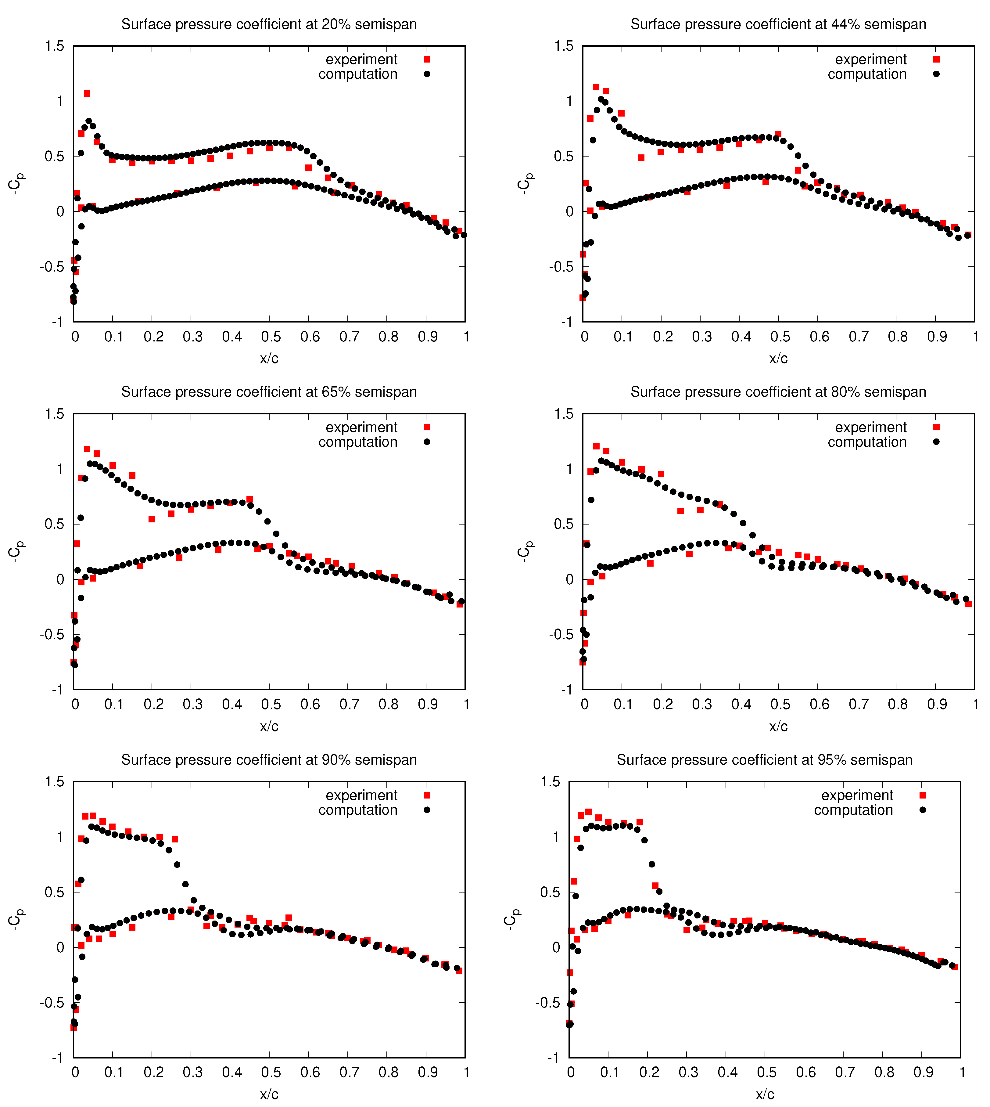
3.2. Validation
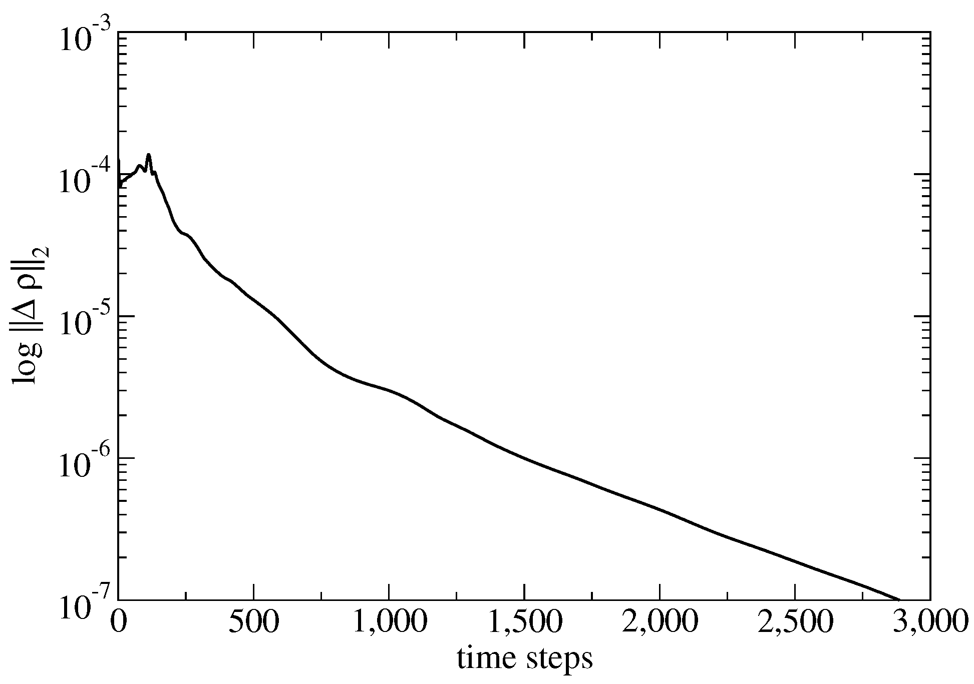
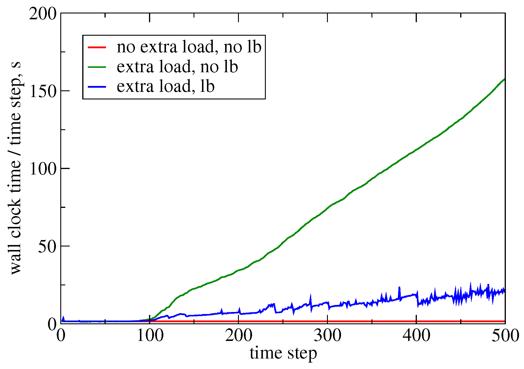
3.3. Automatic Load Balancing
4. Impact and Conclusions
Author Contributions
Funding
Data Availability Statement
Acknowledgments
Conflicts of Interest
References
- Luo, H.; Baum, J.D.; Löhner, R.; Cabello, J. Adaptive Edge-Based Finite Element Schemes for the Euler and Navier-Stokes Equations. In Proceedings of the 31st Aerospace Sciences Meeting, Reno, NV, USA, 1–14 January 1993. [Google Scholar]
- Luo, H.; Baum, J.D.; Löhner, R. Edge-based finite element scheme for the Euler equations. AIAA J. 1994, 32, 1183–1190. [Google Scholar] [CrossRef]
- Waltz, J. Derived data structure algorithms for unstructured finite element meshes. Int. J. Numer. Methods Eng. 2002, 54, 945–963. [Google Scholar] [CrossRef]
- Löhner, R.; Galle, M. Minimization of indirect addressing for edge-based field solvers. Commun. Numer. Methods Eng. 2002, 18, 335–343. [Google Scholar] [CrossRef]
- Löhner, R. Applied Computational Fluid Dynamics Techniques: An Introduction Based on Finite Element Methods; Wiley and Sons Ltd.: Chichester, UK, 2008. [Google Scholar]
- Acun, B.; Gupta, A.; Jain, N.; Langer, A.; Menon, H.; Mikida, E.; Ni, X.; Robson, M.; Sun, Y.; Totoni, E.; et al. Parallel Programming with Migratable Objects: Charm++ in Practice. In Proceedings of the International Conference for High Performance Computing, Networking, Storage and Analysis (SC ’14), New Orleans, LA, USA, 16–21 November 2014; pp. 647–658. [Google Scholar] [CrossRef]
- Waltz, J.; Morgan, N.; Canfield, T.; Charest, M.; Risinger, L.; Wohlbier, J. A three-dimensional finite element arbitrary Lagrangian-Eulerian method for shock hydrodynamics on unstructured grids. Comput. Fluids 2013, 92, 172–187. [Google Scholar] [CrossRef]
- Waltz, J. Microfluidics simulation using adaptive unstructured grids. Int. J. Numer. Methods Fluids 2004, 46, 939–960. [Google Scholar] [CrossRef]
- Davis, S.F. Simplified second-order Godunov-type methods. SIAM J. Sci. Stat. Comput. 1988, 9, 445–473. [Google Scholar] [CrossRef]
- Hirsch, C. Numerical Computation of Internal and External Flows: The Fundamentals of Computational Fluid Dynamics; Wiley and Sons: Chichester, UK; New York, NY, USA; Brisbane, Australia; Toronto, ON, Canada; Singapore, 2007. [Google Scholar]
- Waltz, J.; Canfield, T.; Morgan, N.; Risinger, L.; Wohlbier, J. Manufactured solutions for the three-dimensional Euler equations with relevance to Inertial Confinement Fusion. J. Comput. Phys. 2014, 267, 196–209. [Google Scholar] [CrossRef]
- Luo, H.; Baum, J.; Löhner, R. A Fast, Matrix-Free Implicit Method for Compressible Flows on Unstructured Grids. J. Comput. Phys. 1998, 146, 664–690. [Google Scholar] [CrossRef]
- Schmitt, V.; Charpin, F. Pressure Distributions on the ONERA-M6-Wing at Transonic Mach Numbers, Experimental Data Base for Computer Program Assessment; Report of the Fluid Dynamics Panel Working Group 04; Technical rep4ort, AGARD AR-138; 1979. Available online: https://www.sto.nato.int/publications/AGARD/AGARD-AR-138/AGARD-AR-138.pdf (accessed on 27 March 2023).
- Bakosi, J.; Bird, R.; Gonzalez, F.; Junghans, C.; Li, W.; Luo, H.; Pandare, A.; Waltz, J. Asynchronous distributed-memory task-parallel algorithm for compressible flows on unstructured 3D Eulerian grids. Adv. Eng. Softw. 2021, 160, 102962. [Google Scholar] [CrossRef]
- Li, W.; Luo, H.; Bakosi, J. A p-adaptive Discontinuous Galerkin Method for Compressible Flows using Charm++. In Proceedings of the AIAA Scitech 2020 Forum, Orlando, FL, USA, 6–10 January 2020. [Google Scholar]
- Sedov, L. Similarity and Dimensional Methods in Mechanics, 10th ed.; Elsevier: Amsterdam, The Netherlands, 1993. [Google Scholar] [CrossRef]


| Mesh | Points | Tetrahedra | h |
|---|---|---|---|
| 0 | 132,651 | 750,000 | 0.02 |
| 1 | 1,030,301 | 6,000,000 | 0.01 |
| 2 | 8,120,601 | 48,000,000 | 0.005 |
| Mesh | |||||
|---|---|---|---|---|---|
| 750 K | |||||
| 6 M | |||||
| 48 M | |||||
| Case | Extra Load | Total Time, s | Speed-Up |
|---|---|---|---|
| 0 | no | 825 | - |
| 1 | yes | 30,276 | - |
| 2 | yes | 4958 | 6.11× |
Disclaimer/Publisher’s Note: The statements, opinions and data contained in all publications are solely those of the individual author(s) and contributor(s) and not of MDPI and/or the editor(s). MDPI and/or the editor(s) disclaim responsibility for any injury to people or property resulting from any ideas, methods, instructions or products referred to in the content. |
© 2023 by the authors. Licensee MDPI, Basel, Switzerland. This article is an open access article distributed under the terms and conditions of the Creative Commons Attribution (CC BY) license (https://creativecommons.org/licenses/by/4.0/).
Share and Cite
Bakosi, J.; Constans, M.; Horváth, Z.; Kovács, Á.; Környei, L.; Charest, M.; Pandare, A.; Rutherford, P.; Waltz, J. Complex-Geometry 3D Computational Fluid Dynamics with Automatic Load Balancing. Fluids 2023, 8, 147. https://doi.org/10.3390/fluids8050147
Bakosi J, Constans M, Horváth Z, Kovács Á, Környei L, Charest M, Pandare A, Rutherford P, Waltz J. Complex-Geometry 3D Computational Fluid Dynamics with Automatic Load Balancing. Fluids. 2023; 8(5):147. https://doi.org/10.3390/fluids8050147
Chicago/Turabian StyleBakosi, József, Mátyás Constans, Zoltán Horváth, Ákos Kovács, László Környei, Marc Charest, Aditya Pandare, Paula Rutherford, and Jacob Waltz. 2023. "Complex-Geometry 3D Computational Fluid Dynamics with Automatic Load Balancing" Fluids 8, no. 5: 147. https://doi.org/10.3390/fluids8050147