A Computationally Efficient Dynamic Grid Motion Approach for Arbitrary Lagrange–Euler Simulations

Abstract

The present article addresses the topic of grid motion computation in Arbitrary Lagrange–Euler (ALE) simulations, where a fluid mesh must be updated to follow the displacements of Lagrangian boundaries. A widespread practice is to deduce the motion for the internal mesh nodes from a parabolic equation, such as the harmonic equation, introducing an extra computational cost to the fluid solver. An alternative strategy is proposed to minimize that cost by changing from the parabolic equation to a hyperbolic equation, implementing an additional time derivative term allowing an explicit solution of the grid motion problem. A fictitious dynamic problem is thus obtained for the grid, with dedicated material parameters to be carefully chosen to enhance the computational efficiency and preserve the mesh quality and the accuracy of the physical problem solution. After reminding the basics of the ALE expression of the Navier–Stokes equations and describing the proposed hyperbolic equation for the grid motion problem, the paper provides the necessary characterization of the influence of the fictitious grid parameters and the analysis of the robustness of the new approach compared to the harmonic reference equation on a significant 2D test case. A 3D test case is finally extensively studied in terms of computational performance to highlight and discuss the benefits of the hyperbolic equation for ALE grid motion.

1. Introduction

Modeling the interaction between a fluid flow and a moving structure is essential in understanding a wide range of physical phenomena. In particular, it addresses problems coming from biology, such as the modeling of the cardiovascular system [1,2], as well as many industrial problems coming, for instance, from aeronautics [3,4] or nuclear industry [5,6,7].

Fluid–structure interaction classically requires coupling an Eulerian description for the fluid flow and a Lagrangian description for the structural motion. In many practical situations, the optimum between accuracy, numerical performance, and versatility is achieved through so-called partitioned coupling techniques, implementing a dedicated solver for both fluid and structure components [8,9,10,11]. Whatever the chosen coupling framework, a way to connect Eulerian and Lagrangian descriptions on the fluid–structure interface must be defined. The embedded boundary techniques, where meshes for fluid and structure are topologically disconnected [12,13] provide a set of robust approaches which do not constrain the fluid grid after discretization. The above fluid–structure connections are written in an approximate form, yielding specific issues related to the accuracy of the fluid solution in cells cut by the structural interface [14] that is out of the scope of the present research. On the contrary, following the structural motion for the best representation of fluid phenomena close to the wall precisely imposes switching from a strictly Eulerian description to an intermediate description allowing a moving grid for the fluid. The expansion of the interface motion from the structure to the points inside the fluid domain is arbitrary, with the primary objective of preserving the shapes of the fluid cells along the simulation, thus leading to the Arbitrary Lagrangian-Eulerian (ALE) description of the fluid flow [15].

Using the ALE description, an additional equation is introduced to deduce the motion of the whole fluid grid from the moving boundary conditions. A harmonic equation can easily be implemented for moderate structural motion. For larger displacements, more advanced techniques such as the biharmonic equation [16] or a fictitious elastic model for the grid [17,18] give more robust results. Several comparisons are available in the literature on the mesh motion techniques [19,20] and their impact on the fluid–structure solution [21]. These approaches, however, have all in common the need for an additional solver for the fluid grid introducing an extra computational cost in the fluid solver, related in particular to the solution of a parabolic problem defined on the complete fluid domain.

The purpose of the current paper is thus to propose a new and computationally efficient way to manage the grid problem. It is first implemented for the moderate displacement case, and the article does not aim specifically at enhancing the robustness of the grid motion in the case of large displacements. The proposed approach can, however, easily be derived for any grid motion equation, including those mentioned above, and designed to address the sizeable structural motion case. The idea is to transform the initial parabolic equation into a hyperbolic equation by adding a second-order time derivative that can then be solved with an explicit time integration scheme avoiding any large linear system solution. The computational advantages of the new grid motion algorithm are evaluated on test cases involving the resolution of a simple incompressible flow governed by the Navier–Stokes equation and obtained with TrioCFD open-source software (version 1.8.4, sourced from https://github.com/cea-trust-platform/TrioCFD-code, accessed on 22 August 2022, provided by CEA under BSD license) [22,23]. The physical solution of the tests will not be discussed since the behavior of the code on moving fluid grids is already fully validated for a wide range of flows, including turbulent flows [24,25], and the solution does not depend on the actual grid motion provided the aspect ratio of all cells remain in an acceptable range. On the contrary, the focus is given in the following to assessing the specific behavior of the grid motion resulting from introducing the dynamic term in the arbitrary equation. The proposed grid motion is analyzed in terms of both mesh quality evolution over time and computational efficiency.

The outline of this paper is as follows. Section 2 recalls the principle of the ALE description and its application to Navier–Stokes equations governing the incompressible flow of interest in the paper on a moving mesh. It also recalls the parabolic harmonic equation used for the mesh motion, taken as the reference method, and some short elements describing the time discretization of Navier–Stokes equations implemented in TrioCFD software (version 1.8.4, CEA, Saclay, France). Section 3 explicitly introduces the alternative hyperbolic equation for the mesh motion, with the details of its discretization in both space and time. Finally, Section 4, Section 5 and Section 6 introduce test cases of growing complexity. The simplest case in Section 4 aims at thoroughly understanding and characterizing the influence of the parameters appearing in the new hyperbolic mesh equation. The robustness of the methodology is assessed in Section 5 in a well-known geometric configuration taken from the literature. Finally, Section 6 provides extensive computational performance comparisons in a 3D configuration to highlight the practical benefits of the proposed work.

2. Reminder of Navier–Stokes Equations in ALE Representation

The Navier–Stokes equations are written on a fluid domain ${\Omega }_f$ and the moving motion of the boundary ${\Gamma }_i$ requests, as mentioned above, an ALE description first introduced in the next section, before recalling both the fluid flow governing equations and the mesh motion equation.

It is worth noticing here that the notation ${\Gamma }_i$ classically used to designate a portion of the boundary of domain ${\Omega }_f$ must not be confused with the fluid circulation, also often referenced to with the same symbol.

2.1. ALE Kinematic Description

The ALE description can be found in different sources [15,26,27]. Let ${\Omega }_f\left(t\right)$ be the fluid domain in motion and ${\widehat{\Omega }}_f$ a reference domain. An ALE map application $\mathcal{A}$ is defined as

$$\begin{array}{ccccc}\mathcal{A}& :& {\widehat{\Omega }}_f\times [0,T]& \to & {\Omega }_f\left(t\right)\\ & & (\widehat{\mathbf{x}},t)& \mapsto & (\mathbf{x},t)={\mathcal{A}}_t\left(\widehat{\mathbf{x}}\right).\end{array}$$

(1)

Application $\mathcal{A}$ is a diffeomorphism that allows for equivalence in the definition of fields between the reference domain and the moving domain. The mesh velocity is $\mathit{w}=\frac{\partial }{\partial t}{\mathcal{A}}_t$, $\mathit{F}={\nabla }_{\widehat{\mathit{x}}}{\mathcal{A}}_t$ is the transformation gradient and its determinant is $J=det\left(\mathit{F}\right)$. Defining $\mathit{q}$ a field in the moving domain ${\Omega }_f\left(t\right)$ and $\widehat{\mathit{q}}$ in the referential domain ${\widehat{\Omega }}_f$, both fields are related by

$$\forall \mathit{x}\in {\Omega }_f\left(t\right),\mathit{q}(\mathit{x},t)=\widehat{\mathit{q}}\circ {\mathcal{A}}_t^{-1}\left(\mathit{x}\right)=\widehat{\mathit{q}}\left({\mathcal{A}}_t^{-1}\left(\mathit{x}\right)\right),$$

(2)

$$\forall \widehat{\mathit{x}}\in {\widehat{\Omega }}_f,\widehat{\mathit{q}}(\widehat{\mathit{x}},t)=\mathit{q}\circ {\mathcal{A}}_t\left(\widehat{\mathit{x}}\right)=\mathit{q}\left({\mathcal{A}}_t\left(\widehat{\mathit{x}}\right)\right).$$

(3)

The ALE derivative in time $\frac{\partial }{\partial t}{|}_{\mathcal{A}}$ is introduced as

$$\frac{\partial \mathit{q}}{\partial t}{|}_{\mathcal{A}}(\mathit{x},t)=\frac{\partial \widehat{\mathit{q}}}{\partial t}({\mathcal{A}}_t^{-1}\left(\mathit{x}\right),t)=\frac{\partial \widehat{\mathit{q}}}{\partial t}(\widehat{\mathit{x}},t).$$

(4)

Finally, the following relation between the Eulerian time derivative and the ALE time derivative holds

$$\frac{\partial \mathit{q}}{\partial t}{|}_{\mathcal{A}}(\mathit{x},t)=\frac{\partial \mathit{q}}{\partial t}(\mathit{x},t)+(\mathit{w}(\mathit{x},t)·\nabla )\mathit{u}(\mathit{x},t).$$

(5)

2.2. Standard Navier–Stokes Equations

The fluid is assumed to be homogeneous, Newtonian, and incompressible. The flow is characterized by its velocity $\mathit{u}:{\widehat{\Omega }}_f\times [0,T]\to {\mathbb{R}}^n$ and its pressure $p:{\widehat{\Omega }}_f\times [0,T]\to \mathbb{R}$ and governed by the following Navier–Stokes equations (in Eulerian form)

$$\left\{\begin{array}{cc}\hfill & \nabla ·\mathit{u}=0\mathrm{in}{\widehat{\Omega }}_f,\\ \hfill & {\displaystyle {\rho }_f\frac{\partial \mathit{u}}{\partial t}+{\rho }_f(\mathit{u}·\nabla )\mathit{u}-\nabla ·{\mathit{\sigma }}_f(\mathit{u},p)=\mathbf{0}\mathrm{in}{\widehat{\Omega }}_f.}\end{array}\right.$$

(6)

where ${\rho }_f$ is the density of the fluid, ${\mathit{\sigma }}_f=-p{\mathcal{I}}_d+2{\mu }_f\mathit{ϵ}\left(\mathit{u}\right)$ is the fluid Cauchy stress tensor with ${\mu }_f$ the fluid dynamic viscosity and $\mathit{ϵ}(\mathit{u})=\frac{1}{2}(\nabla \mathit{u}+\nabla {\mathit{u}}^T)$.

2.3. Navier–Stokes Equation in ALE Form

The ALE form of the Navier–Stokes equations is based on the relation between the Eulerian and ALE (5). Introducing the ALE time derivative (still in Eulerian coordinate) yields

$$\left\{\begin{array}{cc}\hfill & \mathit{w}=\mathbf{EXT}\left({\mathit{w}}_{|{\Gamma }_i}\right),\\ \hfill & \nabla ·\mathit{u}=0\mathrm{in}{\Omega }_f\left(t\right),\\ \hfill & {\displaystyle {\rho }_f\frac{\partial \mathit{u}}{\partial t}{|}_{\mathcal{A}}+{\rho }_f(\mathit{u}-\mathit{w})·\nabla \mathit{u}-\nabla ·{\mathit{\sigma }}_f(\mathit{u},p)=\mathbf{0}\mathrm{in}{\Omega }_f\left(t\right).}\end{array}\right.$$

(7)

where EXT denotes any reasonable extension operator of the velocity at the interface ${\Gamma }_i$ in the fluid domain. This formulation is called non-conservative form, from which the conservative form can be derived (see [2,26])

$$\left\{\begin{array}{cc}\hfill & \mathit{w}=\mathbf{EXT}\left({\mathit{w}}_{{\Gamma }_i}\right),\\ \hfill & \nabla ·\mathit{u}=0\mathrm{in}{\Omega }_f\left(t\right)\\ \hfill & {\displaystyle {\rho }_f\frac{\partial J\mathit{u}}{\partial t}{|}_{\mathcal{A}}+J\left[\nabla ·\left(\mathit{u}\otimes (\mathit{u}-\mathit{w}){\rho }_f\right)-\nabla ·{\mathit{\sigma }}_f(\mathit{u},p)\right]=\mathbf{0}\mathrm{in}{\Omega }_f\left(t\right).}\end{array}\right.$$

(8)

Developing the expression and using the definition of ${\mathit{\sigma }}_f$ give the final expression used for discretization

$$\left\{\begin{array}{cc}\hfill & \mathit{w}=\mathbf{EXT}\left({\mathit{w}}_{{\Gamma }_i}\right),\\ \hfill & \nabla ·\mathit{u}=0\mathrm{in}{\Omega }_f\left(t\right),\\ \hfill & {\displaystyle {\rho }_f\frac{\partial J\mathit{u}}{\partial t}{|}_{\mathcal{A}}+J\left[({\rho }_f\left[(\mathit{u}·\nabla )\mathit{u}-(\mathit{w}·\nabla )\mathit{u}\right]-{\mu }_f\Delta \mathit{u}+\nabla p\right]=\mathbf{0}\mathrm{in}{\Omega }_f\left(t\right).}\end{array}\right.$$

(9)

2.4. Additional Mesh Equation

Among the numerous techniques found in the literature to expand the motion imposed by a Lagrangian border to a fluid grid, one frequently encountered and easy to implement is the Harmonic equation, appearing in many fluid–structure interaction studies [9,28]. The velocity is computed by solving the system

$$\left\{\begin{array}{cc}\hfill & -\Delta \mathit{w}=0\mathrm{in}{\Omega }_f\left(t\right),\\ \hfill & \mathit{w}={\mathit{w}}_{{\Gamma }_i}\mathrm{on}{\Gamma }_i\left(t\right).\end{array}\right.$$

(10)

This equation currently exhibits two main drawbacks. The first one is that it does not support large displacements, potentially leading to excessively deformed mesh cells. This can be avoided by switching to a biharmonic equation [16] or a fictitious elastic model affected by the grid [17,18,20]. These solutions are significantly more challenging to implement than the harmonic equation and a comparison between these models is available in [19]. Addressing this topic is outside the scope of the current paper. The second problem, common to all approaches above relying on parabolic equations, is, on the contrary, the specific object of the article and comes from the need for the implicit solution of an additional solver over the complete fluid grid. It induces an additional computational cost of the same order of magnitude as the cost related to the physical solver, and the article’s purpose is thus reduce it drastically under the obvious constraint of preserving the accuracy of the physical solution.

2.5. Discretization of Navier–Stokes Equations

The current introductive section is closed by providing insights regarding the solution of the ALE Navier–Stokes equations, implemented in TrioCFD open-source software (version 1.8.4, CEA, Saclay, France) [22]. Space discretization of (9) is based on the hybrid Finite Element-Volume method for tetrahedral grids [23]. The discretization operators are given by $D,M,A,L\left(\mathit{u}\right)$, and G, corresponding to the discrete divergence, the mass matrices, non-linear diffusion and gradient matrix operators. The expression of these matrices can be found in [29]. Time discretization is performed through an implicit Euler scheme. System (9) then writes

$$\left\{\begin{array}{cc}\hfill & \nabla ·{\mathit{u}}^{n+1}=0\mathrm{in}{\Omega }_f\left(t\right),\\ \hfill & {\displaystyle M\frac{J^{n+1}{\mathit{u}}^{n+1}-J^n{\mathit{u}}^n}{\Delta t_f}+J^{n+1}\left[\right(L\left({\mathit{u}}^n\right){\mathit{u}}^{n+1}-L\left({\mathit{u}}^n\right){\mathit{w}}^{n+1}}\\ \hfill & {\displaystyle -A{\mathit{u}}^{n+1}+G{\mathit{p}}^{n+1}]=\mathbf{0}\mathrm{in}{\Omega }_f\left(t\right).}\end{array}\right.$$

(11)

With ${\mathit{u}}^{n+1},{\mathit{w}}^{n+1},p^{n+1}$ the discrete fluid velocity, mesh velocity, and pressure respectively.

The time step for the fluid is $\Delta t_f$. In TrioCFD, a multi-step technique projection-correction [30,31] is use to solve the system (11).

In order to reduce the computation cost of solving a parabolic equation for the grid motion, the proposed alternative is to transform it into a hyperbolic equation that can be explicitly solved.

2.6. Hyperbolic Equation for the Grid Motion

Starting from the parabolic harmonic equation, a hyperbolic equation is derived by adding a second-order time dependency, transforming the grid motion problem from a quasi-static problem to a wave propagation problem with imposed displacement at the boundary. The new equation writes

$$\frac{{\partial }^2\mathit{w}}{\partial t^2}-c_g^2\Delta \mathit{w}=\mathbf{0}\mathrm{in}{\Omega }_f\left(t\right),$$

(12)

where $c_g$ is the wave velocity.

This approach inherits from structural dynamics and introduces new pseudo-physical parameters to adjust and control the dynamic response of the grid, namely the fictitious density ${\rho }_g$ and the fictitious stiffness $k_g$ of the grid. These parameters are related to the wave velocity through the relation $c_g=\sqrt{\frac{k_g}{{\rho }_g}}$, yielding

$${\rho }_g\frac{{\partial }^2\mathit{w}}{\partial t^2}-k_g\Delta \mathit{w}=\mathbf{0}\mathrm{in}{\Omega }_f\left(t\right).$$

(13)

Finally, a damping coefficient $d_g$ is added to the model to help control its response further so that the complete hyperbolic equation to consider for the grid is

$$\left\{\begin{array}{cc}\hfill & {\displaystyle {\rho }_g\frac{{\partial }^2\mathit{w}}{\partial t^2}+d_g\frac{\partial \mathit{w}}{\partial t}-k_g\Delta \mathit{w}=\mathbf{0}\mathrm{in}{\Omega }_f\left(t\right),}\\ \hfill & \mathit{w}={\mathit{w}}_{{\Gamma }_i}\mathrm{on}{\Gamma }_i\left(t\right),\\ \hfill & \mathit{w}=\mathbf{0}\mathrm{on}\partial {\Omega }_f\left(t\right)\setminus {\Gamma }_i\left(t\right),\end{array}\right.$$

(14)

with ${\mathit{w}}_{{\Gamma }_i}$ a specified velocity of the moving border.

2.7. Weak Form of the Hyperbolic Grid Motion Problem

Introducing $V=H^1(\Omega )$ and $\mathit{V}={\left(H^1(\Omega )\right)}^3$, the weak form of the previous problem is classically obtained by multiplying (14) by a test function $\mathit{v}\in {\left(H_0^1\left({\Omega }_f\right)\right)}^3$ and integrating on the domain, resulting in

$${\rho }_g{\int }_{{\Omega }_f}\frac{{\partial }^2\mathit{w}}{\partial t^2}·\mathit{v}d\mathit{x}+d_g{\int }_{{\Omega }_f}\frac{\partial \mathit{w}}{\partial t}·\mathit{v}d\mathit{x}+k_g{\int }_{{\Omega }_f}\Delta \mathit{w}·\mathit{v}d\mathit{x}=\mathbf{0}.$$

(15)

Using the Green formula and assuming ${\mathit{v}}_{|\partial {\Omega }_f}=\mathbf{0}$ yields the expected weak form to be discretized in the next section:

Find $\mathit{w}\in \mathit{V}$ with $\mathit{w}={\mathit{w}}_{{\Gamma }_i}$ on ${\Gamma }_i$, such that

$$\forall \mathit{v}\in {\left(H_0^1\left({\Omega }_f\right)\right)}^3,{\rho }_g{\int }_{{\Omega }_f}\frac{{\partial }^2\mathit{w}}{\partial t^2}·\mathit{v}d\mathit{x}+d_g{\int }_{{\Omega }_f}\frac{\partial \mathit{w}}{\partial t}·\mathit{v}d\mathit{x}+k_g{\int }_{{\Omega }_f}\nabla \mathit{w}:\nabla \mathit{v}d\mathit{x}=\mathbf{0}.$$

(16)

2.8. Space Discretization

Given a triangulation ${\mathcal{T}}_h$ of the domain ${\Omega }_f$ with $h\in ]0,1]$ a distance referring to the level of refinement, ${\mathcal{T}}_h$ is associated to a vector subspace $V_h\subset V$ which is the approximation of the space solution such that

$$\underset{h\to 0}{lim}{V}_h=V.$$

(17)

A ${\mathbb{P}}_1$ finite element approximation and the corresponding shape functions ${\left\{{\varphi }_i\right\}}_{i=1,\cdots ,N_h}$ are used to define $V_h$ a space of dimension $N_h$

$$V_h=\{v_h\in C^0(\Omega )|v_h{|}_{\tau }\in {\mathbb{P}}_1\forall \tau \in {\mathcal{T}}_h\}.$$

(18)

One approximate field then can be expressed by a projection onto the created subspace with the new unknowns $({\mathit{\alpha }}_{h,1}\left(t\right),\cdots ,{\mathit{\alpha }}_{h,N_h}\left(t\right))$

$$\forall (t,\mathit{x})\in ([t_0,t_{max}]\times {\Omega }_f),{\mathit{w}}_h(t,x)=\sum _{i=1}^{N_h}{\mathit{\alpha }}_{h,i}\left(t\right){\varphi }_i\left(\mathit{x}\right).$$

(19)

Each unknown is a vector corresponding to the three directions of space, ${\mathit{\alpha }}_{h,i}={({\alpha }_{h,i}^x,{\alpha }_{h,i}^y,{\alpha }_{h,i}^z)}^T$. Injecting the decomposition (19) of ${\mathit{w}}_h$ into the weak form (16) produces

$$\begin{array}{cc}\hfill & {\displaystyle {\rho }_g{\int }_{{\Omega }_f}\frac{{\partial }^2}{\partial t^2}\left(\sum _{i=1}^{N_h}{\mathit{\alpha }}_{h,i}{\varphi }_i\right)·\mathit{v}d\mathit{x}+d_g{\int }_{{\Omega }_f}\frac{\partial }{\partial t}\left(\sum _{i=1}^{N_h}{\mathit{\alpha }}_{h,i}{\varphi }_i\right)·\mathit{v}d\mathit{x}}\\ \hfill & {\displaystyle +k_g{\int }_{{\Omega }_f}\nabla \left(\sum _{i=1}^{N_h}{\mathit{\alpha }}_{h,i}{\varphi }_i\right):\nabla \mathit{v}d\mathit{x}=\mathbf{0}.}\end{array}$$

(20)

Using the linearity of the differential operators and setting $\mathit{v}=\mathbb{1}{\varphi }_j$ with $j=0,\cdots ,N_h$

$$\begin{array}{cc}\hfill & {\displaystyle {\rho }_g\sum _{i=1}^{N_h}\frac{{\partial }^2}{\partial t^2}{\mathit{\alpha }}_{h,i}·\mathbb{1}{\int }_{{\Omega }_f}{\varphi }_i{\varphi }_{j}d\mathit{x}+d_g\sum _{i=1}^{N_h}\frac{\partial }{\partial t}{\mathit{\alpha }}_{h,i}·\mathbb{1}{\int }_{{\Omega }_f}{\varphi }_i{\varphi }_{j}d\mathit{x}}\\ \hfill & {\displaystyle +k_g\sum _{i=1}^{N_h}{\mathit{\alpha }}_{h,i}·\mathbb{1}{\int }_{{\Omega }_f}\nabla {\varphi }_i·\nabla {\varphi }_{j}d\mathit{x}=\mathbf{0}.}\end{array}$$

(21)

This introduces the mass, damping, and stiffness matrices defined as

$$\begin{array}{cc}& {\displaystyle {\left(M_h\right)}_{ij}={\left(D_h\right)}_{ij}={\int }_{\Omega }{\varphi }_i{\varphi }_{j}d\mathit{x},}\\ & {\displaystyle {\left(K_h\right)}_{ij}={\int }_{\Omega }\nabla {\varphi }_i·\nabla {\varphi }_{j}d\mathit{x}.}\end{array}$$

(22)

Space discretization is then concluded by writing the system (21) in matrix form

$$\begin{array}{cc}\hfill & {\displaystyle {\rho }_g\left(\begin{array}{ccc}{M}_h& 0& 0\\ 0& M_h& 0\\ 0& 0& M_h\end{array}\right)\frac{{\partial }^2}{\partial t^2}\mathit{W}+d_g\left(\begin{array}{ccc}{D}_h& 0& 0\\ 0& D_h& 0\\ 0& 0& D_h\end{array}\right)\frac{\partial }{\partial t}\mathit{W}}\\ \hfill & {\displaystyle +k_g\left(\begin{array}{ccc}{K}_h& 0& 0\\ 0& K_h& 0\\ 0& 0& K_h\end{array}\right)\mathit{W}=\mathbf{0}.}\end{array}$$

(23)

With the solution vector $\mathit{W}$

$$\mathit{W}=\left[\begin{array}{c}{\left({\alpha }_{h,i}^x\right)}_{i=1,\cdots ,N_h}^T\\ {\left({\alpha }_{h,i}^y\right)}_{i=1,\cdots ,N_h}^T\\ {\left({\alpha }_{h,i}^z\right)}_{i=1,\cdots ,N_h}^T\end{array}\right].$$

(24)

2.9. Time Discretization

The time interval of interest $[0,T]$ is subdivided into smaller intervals such that $t_0=0<t_1<\cdots <t_N=T$ with $\Delta t=t_{n+1}-t_n$. For the sake of clarity, the following notations are now used: ${\mathit{W}}^n=\mathit{W}\left(t_n\right)$, ${\dot{\mathit{W}}}^n=\frac{\partial }{\partial t}{\mathit{W}}^n$ and ${\ddot{\mathit{W}}}^n=\frac{{\partial }^2}{\partial t^2}{\mathit{W}}^n$. Matrix system (23) now writes for one space direction and at time $t_{n+1}$

$${\rho }_g{M}_h{\ddot{\mathit{W}}}^{n+1}+d_g{D}_h{\dot{\mathit{W}}}^{n+1}+k_g{K}_h{\mathit{W}}^{n+1}=\mathbf{0}.$$

(25)

Time derivatives are approximated using the Central Difference explicit scheme from the Newmark family

$$\left\{\begin{array}{ccc}\hfill {\mathit{W}}^{n+1}& \approx & {\mathit{W}}^n+\Delta t{\dot{\mathit{W}}}^n+\frac{\Delta t^2}{2}{\ddot{\mathit{W}}}^n,\hfill \\ \hfill {\dot{\mathit{W}}}^{n+1}& \approx & {\dot{\mathit{W}}}^n+\frac{\Delta t}{2}\left[{\ddot{\mathit{W}}}^{n+1}+{\ddot{\mathit{W}}}^n\right].\hfill \end{array}\right.$$

(26)

This yields a solution procedure in three steps.

(1) Prediction step: Please confirm if the bold should be retained. same as below compute the explicit displacement and a prediction of the mid-step velocity

$$\begin{array}{ccc}\hfill {\dot{\mathit{W}}}^{n+\frac{1}{2}}& =& {\dot{\mathit{W}}}^n+\frac{\Delta t}{2}{\ddot{\mathit{W}}}^n,\hfill \\ \hfill {\mathit{W}}^{n+1}& =& {\mathit{W}}^n+\Delta t{\dot{\mathit{W}}}^{n+\frac{1}{2}}.\hfill \end{array}$$

(27)

(2) Equilibrium solution: compute acceleration from

$${\rho }_g\left(M_h+\frac{\Delta t}{2}{D}_h\right){\ddot{\mathit{W}}}^{n+1}=-\left(d_g{D}_h{\dot{\mathit{W}}}^{n+\frac{1}{2}}+k_g{K}_h{\mathit{W}}^{n+1}\right).$$

(28)

The solution is explicitly provided when the matrices $M_h$ and $D_h$, which have here the same consistent expression (see Equation (23)), are made diagonal through a classical lumping process.

(3) End-of-step velocity update

$${\dot{\mathit{W}}}^{n+1}={\dot{\mathit{W}}}^{n+\frac{1}{2}}+\Delta t{\ddot{\mathit{W}}}^{n+1}.$$

(29)

2.10. Stability Condition for the Explicit Time Integration

The computation of a stability condition of the problem (25) classically involves an eigenvalue problem that is difficult to compute. A sufficient condition for the maximum time step is given by the Courant–Friedrich–Lewy condition (CFL, see, for instance [32]) for a one-dimensional propagation problem

$$\Delta t_{max}\le \frac{h}{c_g}.$$

(30)

Using the relation $c_g=\sqrt{\frac{k_g}{{\rho }_g}}$ yields

$$\Delta t_{max}<\alpha h\sqrt{{\displaystyle \frac{{\rho }_g}{k_g}}},$$

(31)

with $\alpha \in ]0,1[$ a security coefficient, needed to account for the approximate evaluation of the characteristic dimension h of the mesh cells when switching to the multidimensional case. Such a discretization strategy introduces two issues to consider carefully regarding numerical performance.

First, in the general case, during the simulations, the grid stability time step will be smaller than the time step prescribed for the physical fluid problem. In order to avoid penalizing the physical solution with the new grid problem formulation, a subcycling algorithm is implemented.

Second, even if only a matrix-vector product is now required at each time step for the grid motion problem, which is the precise point of switching to a hyperbolic equation, the solution of the grid problem is likely to remain computationally costly if too many subcycles are performed due to a low stability time step. This issue is addressed through the optimal choice of the fictitious mass, stiffness, and damping coefficients from Equation (14). The goal is then to maximize the stability time step with respect to the physical fluid time step while controlling the grid’s dynamic response and preserving the mesh quality.

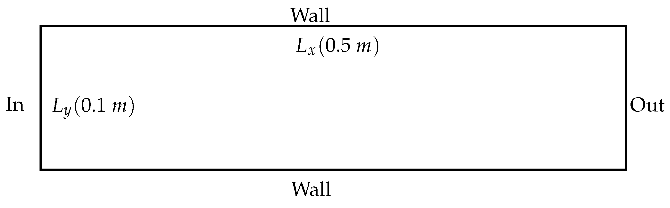
3. Basic Pseudo-1D Test to Characterize the Influence of Fictitious Material Coefficients

3.1. Test Setup

This first test case is straightforward and corresponds to the pseudo-1D compression of a rectangular fluid domain of length $L_x=0.5$ m and height $L_y=0.1$ m. Boundary conditions for the fluid problem are homogeneous Dirichlet conditions for the fluid velocity $\mathit{u}$ at the left (In) and homogeneous Neumann conditions at the right (Out). The setup and the boundary conditions are illustrated in Figure 1. For the grid problem, Equation (14), the compression corresponds to imposing a non-homogeneous Dirichlet condition on the left border and a homogeneous Neumann condition on the walls (up and down border). The domain is first compressed by imposing the motion of the left border with a maximal displacement of $0.05$ m, and it is then stretched back to its original configuration at the same velocity. The period of the border motion is $0.1$ s. Figure 2 shows the compression of the domain during a single period.

3.2. Analysis of the Influence of the Damping Coefficient

For a dynamic system like the one built for the new grid motion problem, the damping is expected to affect the wave traveling in the domain and can be tuned to have them vanish more or less quickly.

For this first analysis, mass and stiffness coefficients are chosen to ${\rho }_g=1000$ kg·m${}^{-3}$ and $k_g={10}^6$ Pa so that the wave velocity is set to $c_g=32$ m·s${}^{-1}$. This relatively low value compared to standard structural dynamics allows clear visualization of the grid motion waves in the computational domain, as illustrated in Figure 3. The effect of the damping coefficient is then relatively straightforward since a value close to zero $(d_g=1$ N·m${}^{-1}$·s) on the left results in significant compression/traction waves traveling in the grid, whereas as a significant value $(d_g={10}^5$ N·m${}^{-1}$·s) efficiently cancels the waves and retrieves a quasi-static motion of the grid in response of the moving boundary. When targetting quasi-static grid motion, a damping coefficient near the stiffness coefficient is the best choice.

3.3. Analysis of the Influence of the Mass and Stiffness Coefficients

Stiffness controls the forces exerted on the mesh nodes in response to the deformation of the mesh cells. Too low a stiffness will concentrate the deformation close to the moving walls, and too high a stiffness will enhance the grid’s dynamic response and lower the stability time step given by the CFL condition. As introduced in the previous paragraph, significant stiffness values are suitably associated with significant damping to prevent grid oscillations far from the imposed motion.

Figure 4 displays the largest internal angle for each mesh triangle at the maximum compression of the domain ( time $t=0.05$ s) for three values of the stiffness coefficients $k_g\in \{{10}^4,{10}^6,{10}^8\}$ Pa and the same density coefficient $({\rho }_g={10}^4$ kg·m${}^{-3}$). A high maximum internal angle for a triangle corresponds to an element with a bad aspect ratio. It could therefore impact the quality of the physical solution or even lead the simulation to stop. It is easily observed that the lowest stiffness coefficient excessively localizes the deformation close to the moving wall as expected. The global mesh motion becomes acceptable with the intermediate stiffness value, and the improvement provided by the highest value thus does not compensate for the additional penalization induced on the stability time step, ten times smaller following Equation (31).

Figure 5 shows the results for the same configurations as above, but at the final time, where the moving wall is back at its initial location. The observations are the same as before; only the mesh cells are elongated instead of crushed. At this time, only the highest stiffness coefficient leads to the grid returning to its initial shape. A slight residual shift is observed with a softer grid ($k_g={10}^6$ Pa), suggesting a low-frequency oscillation of the grid if the simulation is continued. However, the amplitude of the latter is moderate and does not affect the quality of the physical solution, highlighting the choice left to the users for the optimum trade-off between numerical performance (i.e., highest possible stability time step) and controlled grid motion.

Finally, Figure 6 shows the influence of the density coefficient affected the grid, with values ${\rho }_g\in \{{10}^3,{10}^4,{10}^5\}$ kg·m${}^{-3}$ used jointly with a stiffness coefficient $k_g={10}^6$ Pa. In this case, the chosen density has a minimal effect on the shapes of the mesh cells at maximum grid compression, which can be attributed to the relatively slow wall motion. It must, however, be recalled that increasing the grid density also improves the stability time step.

4. 2D Test Case Derived from Turek’s Benchmark with Imposed Motion

The previous section analyzed the influence of the different parameters of Equation (14), emphasizing the importance of the damping coefficient and a well-chosen stiffness. It is essential to choose the stiffness carefully to obtain both a qualitative grid movement and the least restrictive CFL condition. Thus, this section compares two grids, one soft and one stiff, with the results obtained from the harmonic Equation (10).

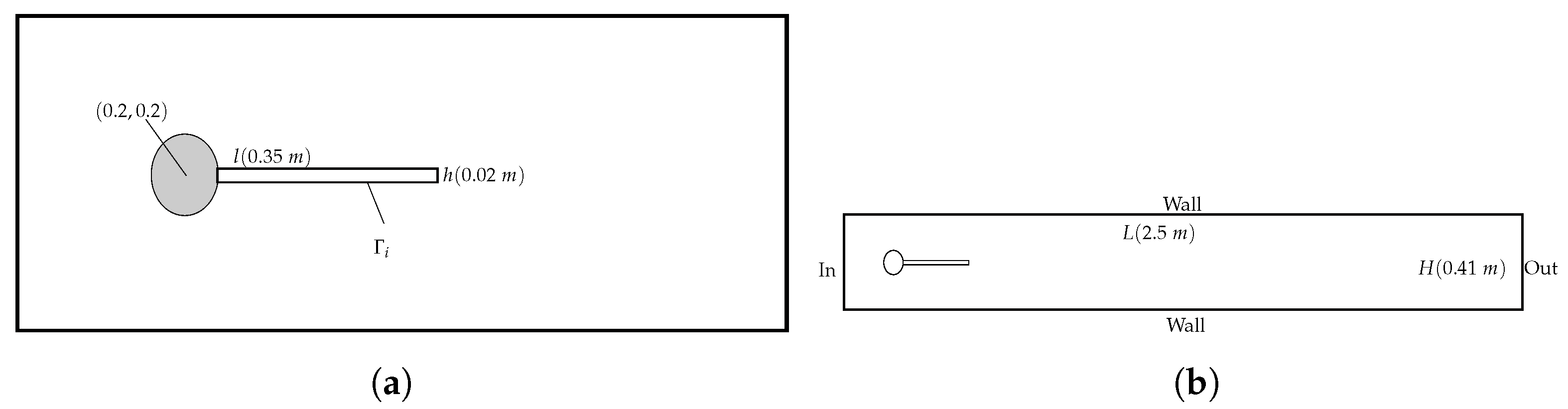
4.1. Presentation of the Turek Test Case

The Turek benchmark is a classical validation test case for fluid–structure interaction solvers [33,34]. In this test case, the fluid flows around an elastic obstacle clamped to a rigid stationary cylinder (see Figure 7). The fluid domain length is $L=2.5$ m, and its height is $H=0.41$ m. The cylinder center coordinates are $(0.2,0.2)$ m, and its radius is $0.05$ m. The elastic structure, denoted by ${\Gamma }_i$ has length $l=0.35$ m and height $h=0.02$ m.

4.2. Boundary Conditions and Parameters

The fluid is initially at rest, ${\Gamma }_i$ is flexible, and points on its lateral boundary are imposed a simple harmonic displacement of the form $w_{{\Gamma }_i}=\left(0,\varphi \left(x\right)\right)$, with

$$\varphi \left(x\right)=\gamma \sum _{i=1}^k\frac{{\alpha }_i}{sup|V_i|}{V}_i\left(x\right)cos\left({\omega }_{i}t\right),$$

(32)

where $\gamma$ is the amplitude of the displacement, x the longitudinal coordinate, $V_i\left(x\right)$ is the i-th bending mode of vibration of an Euler-Bernoulli beam with clamped-free boundary conditions, and $N_i=sup\left(\left|V_i\left(x\right)\right|,x\in \left[0,l\right]\right)$ its infinite norm, ${\omega }_i$ the angular frequency, t the time and ${\sum }_{i=1}^k{\alpha }_i=1$. The elastic obstacle is referred to as the beam from now on.

Two sets of properties are considered for the hyperbolic grid motion: one called soft and the other called stiff. The damping coefficients are set according to the previous analysis, and all the parameters are summarized in

Table 1. Grids parameters of the Turek test case.

	${\mathit{\rho }}_{\mathit{g}}$	${\mathit{k}}_{\mathit{g}}$	${\mathit{d}}_{\mathit{g}}$	$\mathbf{\Delta }\mathit{t}$
Stiff grid	${10}^3$	${10}^8$	${10}^7$	∼$\left[1\times {10}^{-6},2\times {10}^{-6}\right]$
Soft grid	${10}^3$	${10}^6$	${10}^6$	∼$\left[1\times {10}^{-5},2\times {10}^{-5}\right]$

. A locally refined grid with ${10}^4$ triangles is used. Two different local sizes are defined in the meshing process: a small local size of $25\times {10}^{-4}$ m for elements close to the beam and a large global size $25\times {10}^{-3}$ m elsewhere. The fluid time step, $\Delta t_f$, is fixed to $2\times {10}^{-4}$. The grid time step varies between $1\times {10}^{-5}$ s and $2\times {10}^{-5}$ s for the soft grid and between $1\times {10}^{-6}$ s and $2\times {10}^{-6}$ s for the stiff grid (ten times lower in agreement with the same density and a stiffness multiplied by 100 for the soft grid).

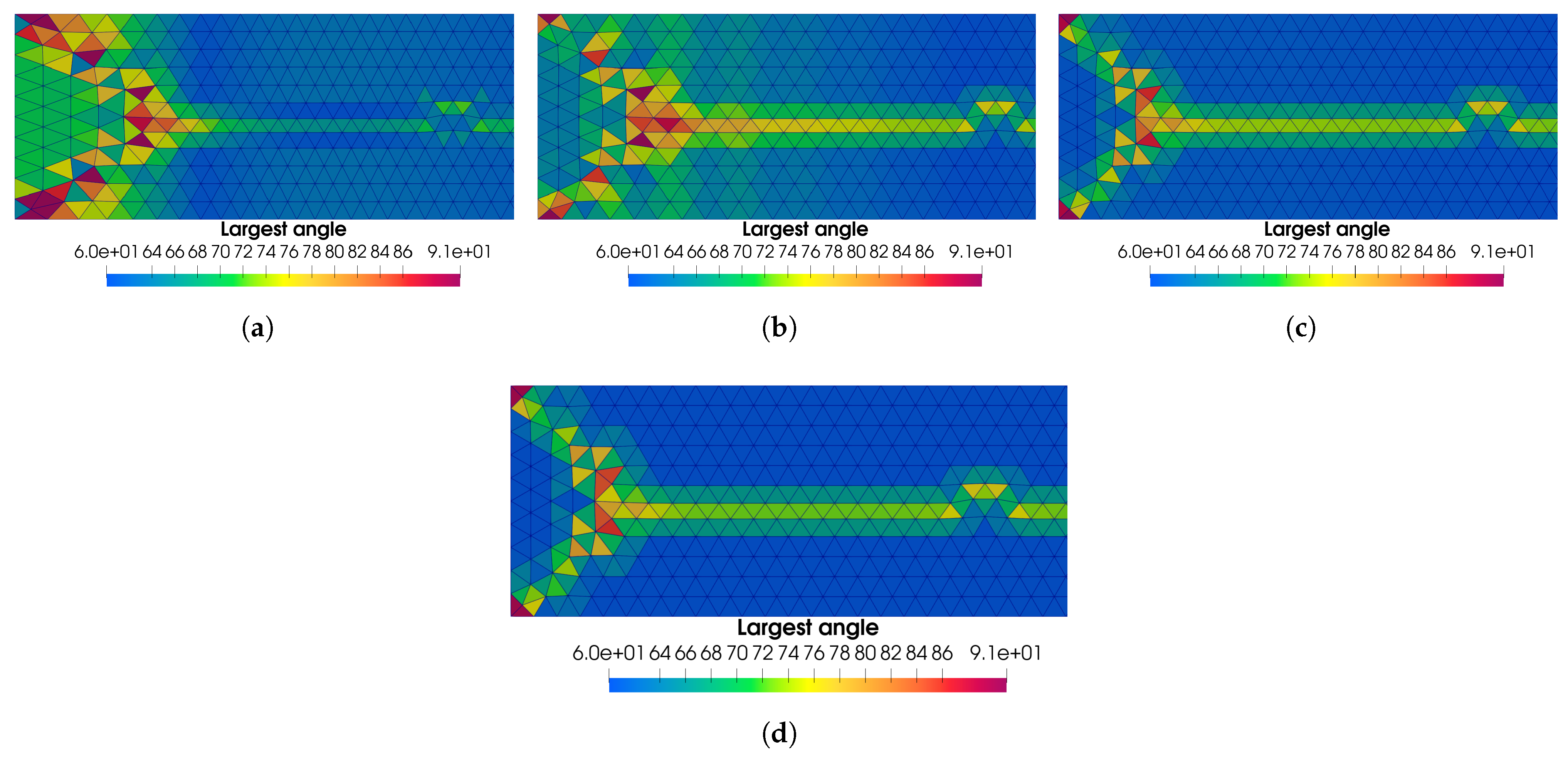
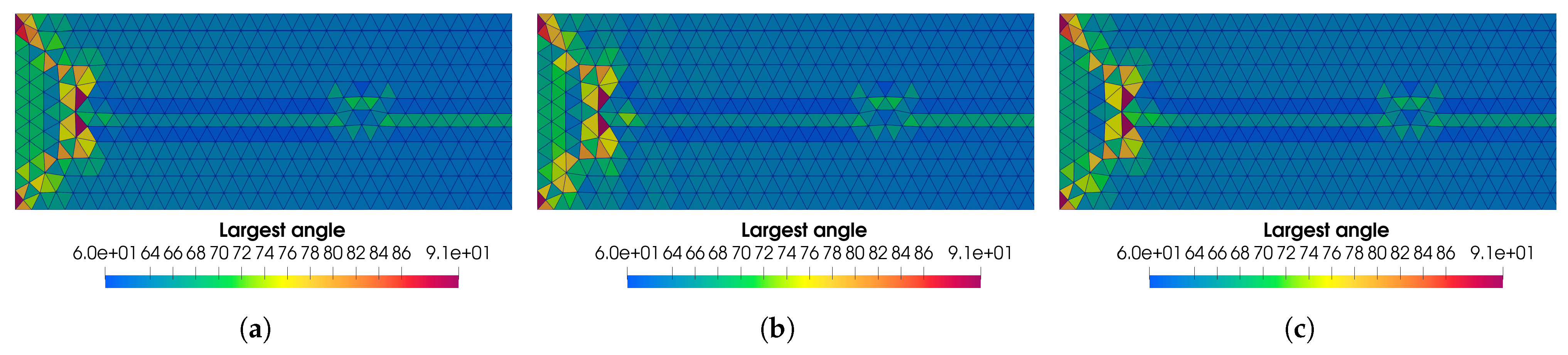
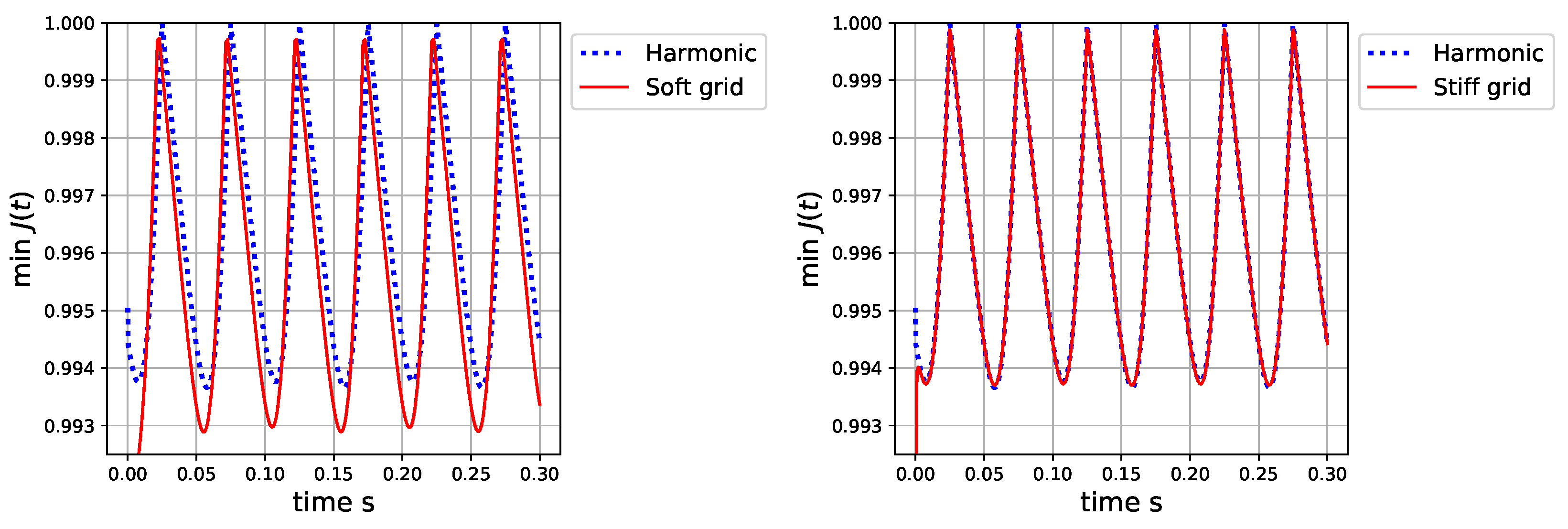
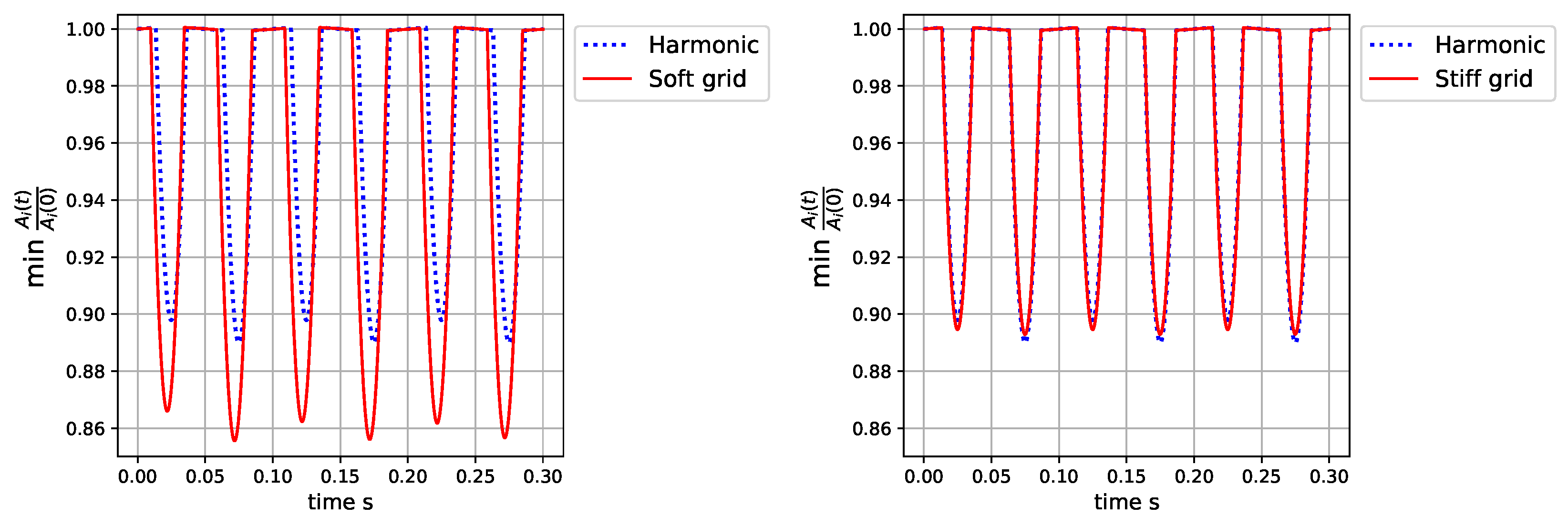
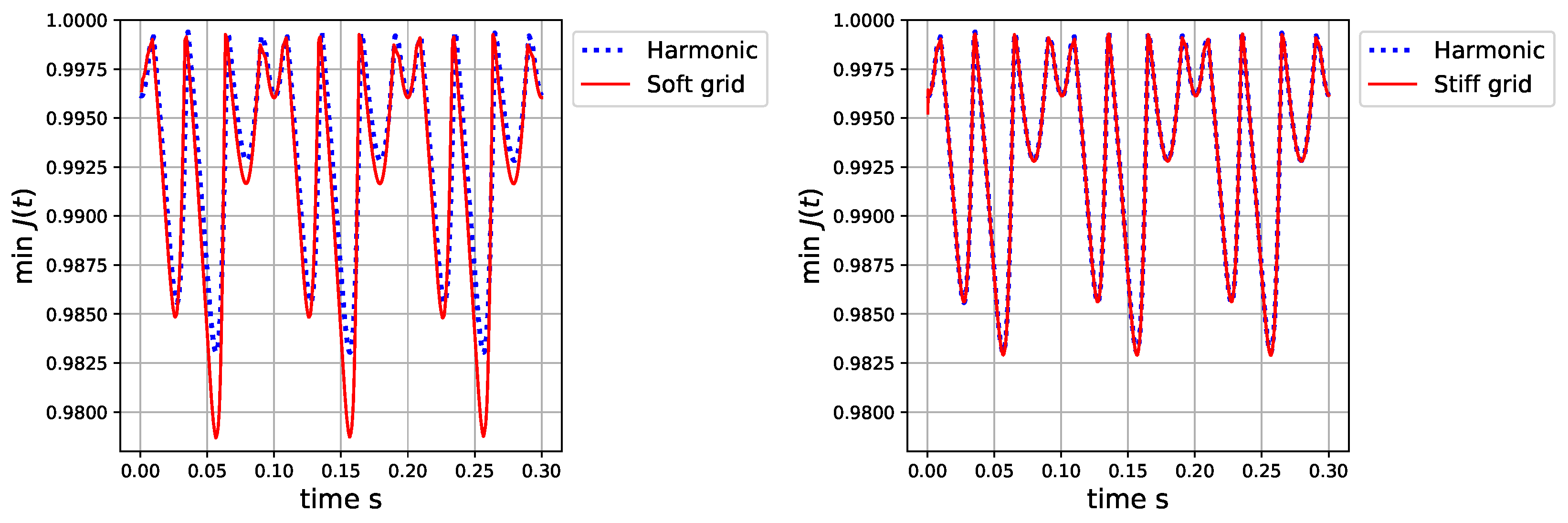
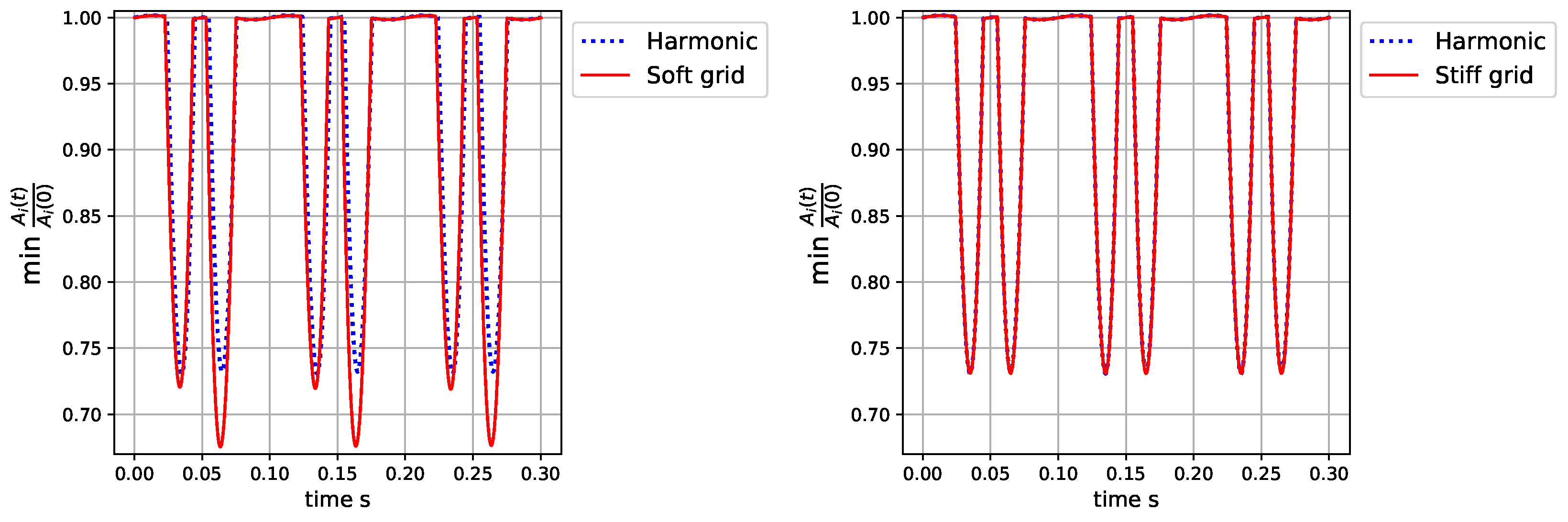
4.3. Analysis through a Comparison with the Harmonic Grid Motion

In this section, the dynamics of the two grids (stiff and soft) is analyzed through a comparison with the motion of the harmonic grid, described by Equation (10). As a first step, only the first bending mode of vibration of the clamped-free beam (i.e., $k=1$ in Equation (32)) is considered. The displacement amplitude is set to $\gamma =0.15$ m, and the imposed frequency is $\omega /\left(2\pi \right)=10$ Hz. Figure 8 illustrates the dynamics of the beam at different time steps.

Figure 9 plots the evolution of the minimum of the Jacobian determinant, J. The evolution of J represents a criterion of the quality of the mesh. Thus, the decrease of J denotes a degradation of the quality of the meshes. For the stiff grid, the curve fits perfectly with the minimum of the Jacobian determinant obtained with the harmonic equation. For the soft grid, a shift is observed. The minimum values of the curve are lower than that of the harmonic equation, which indicates a moderate extra-degradation of the grid quality. However, the minimum of the Jacobian determinant remains periodic and comes back close to 1 after each period, so the grid motion remains consistent with the harmonic equation.

Figure 10 plots the normalized minimum area cell’s grid evolution. As before, the stiff grid fits perfectly with the harmonic mesh movement, while the soft grid presents a shift. Soft grid cells have a smaller minimum area than harmonic grid cells. As a result, the soft grid is less accurate when the beam reaches its maximum amplitude. Despite this, the cells do not degenerate and return to their original shape at the end of each period, so the soft grid remains consistent for computations. Similarly, both quantities suggest that the motion of a still grid is close to the harmonic grid behavior.

Figure 11 and Figure 12, show how grid behavior evolves as beam motion is varied. The displacement imposed on the beam is calculated by considering the two first vibration modes of the clamped-free beam, i.e., $k=2$ in Equation (32). The amplitude of the displacement is $\gamma =0.15$ m, the imposed frequency are ${\omega }_1/\left(2\pi \right)=10$ Hz and ${\omega }_2/\left(2\pi \right)=20$ Hz, and the weight coefficients ${\alpha }_1=0.7$ and ${\alpha }_2=0.3$. Observations remain the same. The comparison with the harmonic grid remains unchanged even when additional vibration modes are considered, i.e., $k>2$ in Equation (32).

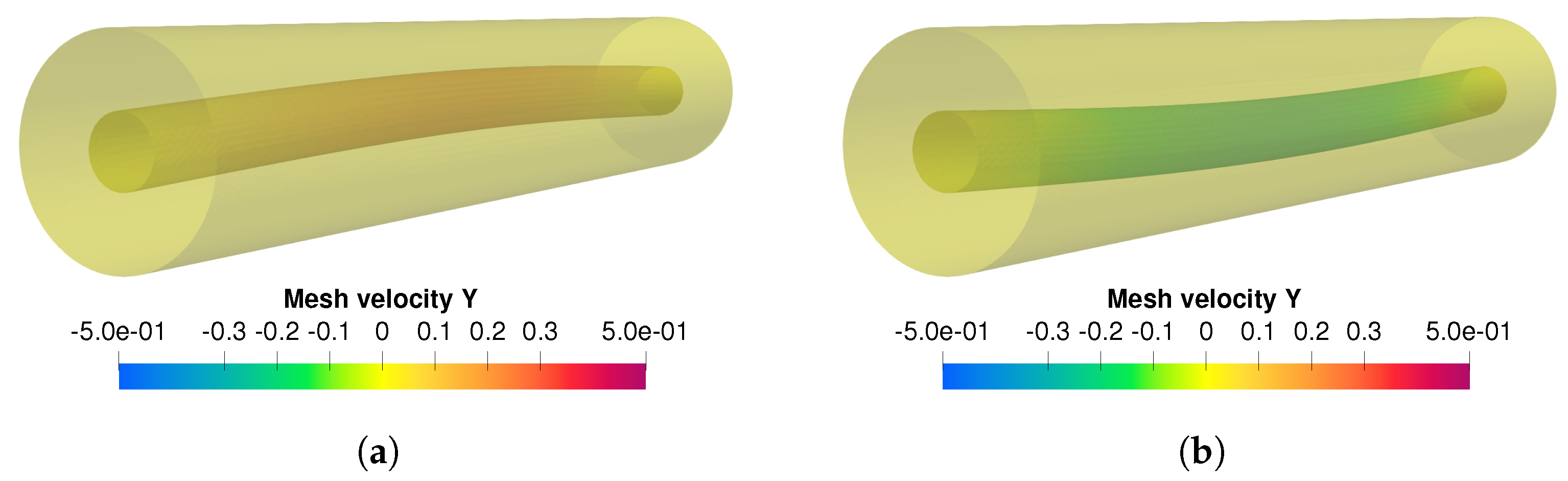
5. 3D Test Case for Computational Performance Analysis

The previous section discussed the effect of fictitious material coefficients in Equation (14) on the grid motion resulting from the hyperbolic problem. Afterward, the purpose of this section is to discuss the computational performance benefits of the proposed approach on significant meshes. A 3D configuration and intermediate mesh sizes (i.e., up to 2 million cells) are chosen to simultaneously exhibit reliable measures and tendencies for computational times and allow the consideration of several meshes and set of parameters in a reasonable time.

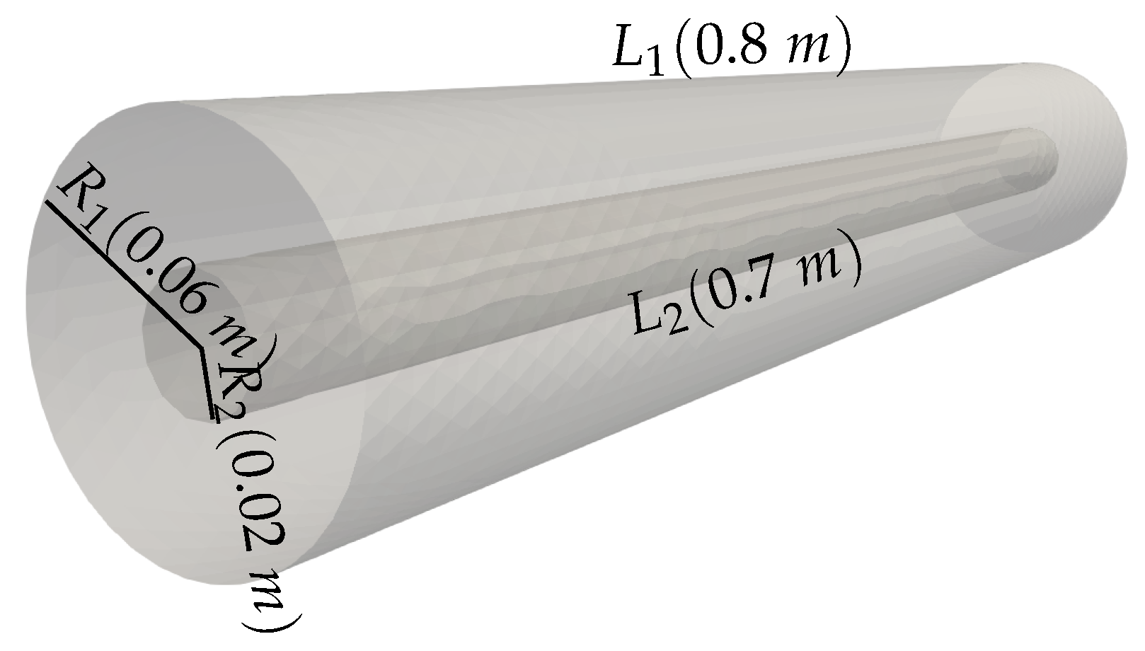
5.1. Description of the Test Case and Computational Parameters

The problem is three-dimensional, consisting of two coaxial cylinders separated by a fluid layer initially at rest. The external cylinder is rigid and fixed. The inner cylinder is flexible, and as in the previous section, points on its lateral boundary are imposed, on the $e_y$ direction, a simple harmonic displacement of the form

$$\varphi \left(x\right)=\gamma sin\left(\pi x/L\right)cos\left(\omega t\right),$$

(33)

corresponding to the first bending mode of vibration of an Euler-Bernoulli beam with pinned-pinned boundary conditions. The radii are $R_1=0.06$ m and $R_2=0.02$ m, and the lengths are $L_1=0.8$ m and $L_2=0.7$ m, the setup is illustrated in Figure 13. The simulations are performed with an imposed displacement of amplitude $\gamma =0.15$ m and a forcing frequency $\omega /\left(2\pi \right)=10$ Hz. Figure 14 shows the displacement of the pinned-pinned cylinder.

The case is solved with TrioCFD using a classic and efficient combination of solvers and algorithmic options for this problem, with results discussed in the next section. The time integration is here implicit for the velocity. The velocity problem is solved through the GMRES algorithm implemented in the program, whereas the pressure problem solution is obtained through the Preconditioned Conjugate Gradient (PCG) algorithm from the PETSc library (see https://petsc.org, accessed on 22 August 2022). The latter is used for the grid motion computed with the harmonic equation. All the simulations are performed using parallel processing and 8 Core Processing Units.

5.2. Analysis of the Computational Performance for the Grid Problem Solution

As a preamble to this section, it is essential to remark that the fraction of the total time of the simulations taken by the grid motion problem depends on many parameters associated with the solution of Navier–Stokes equations. It is, in particular, influenced by the choice between implicit and explicit time integration for the convective velocity problem. Moreover, the approach proposed in the current paper could also indifferently be applied to other sets of ALE equations, such as Euler equations for compressible fluids, with again another ratio between the time needed to update the grid and the total computation time. Hence, the focus is more oriented toward the performance of the grid motion solver itself, even if some insights regarding the influence of the fictitious grid parameters on the performance of the global fluid problem solution are also provided.

Four meshes with respectively $0.5$, $1.$, $1.5$, and $2.$ million tetrahedra are considered for the fluid domain. For the sake of simplicity, two already defined sets of fictitious grid parameters are selected for the cases with mesh motion solved by the new hyperbolic equation. They are labeled soft and stiff according to Table 1 in Section 4.2. Indicative time step ratios between the chosen fluid solver and the hyperbolic grid problem are given in

Table 2. Indicative time step ratios between the fluid problem and the hyperbolic problems for the selected fictitious grid parameters.

	Mesh 1	Mesh 2	Mesh 3	Mesh 4
Nb elements	$0.5\times {10}^6$	${10}^6$	$1.5\times {10}^6$	$2\times {10}^6$
$\Delta t_f$	$5.39\times {10}^{-4}$	$3.14\times {10}^{-4}$	$3.00\times {10}^{-4}$	$2.88\times {10}^{-4}$
$\Delta t$  soft   grid	$1.11\times {10}^{-5}$	$7.94\times {10}^{-6}$	$6.95\times {10}^{-6}$	$6.46\times {10}^{-6}$
$\Delta t$  stiff   grid	$1.11\times {10}^{-6}$	$7.94\times {10}^{-7}$	$6.95\times {10}^{-7}$	$6.46\times {10}^{-7}$
$\mathbf{Ratio} \mathit{soft} \mathbf{grid}$	49	40	43	45
$\mathbf{Ratio} \mathit{stiff} \mathbf{grid}$	486	395	431	446

. The fictitious speeds of sound for both grids, needed in the next section, are 32 m·s${}^{-1}$ and 316 m·s${}^{-1}$, respectively.

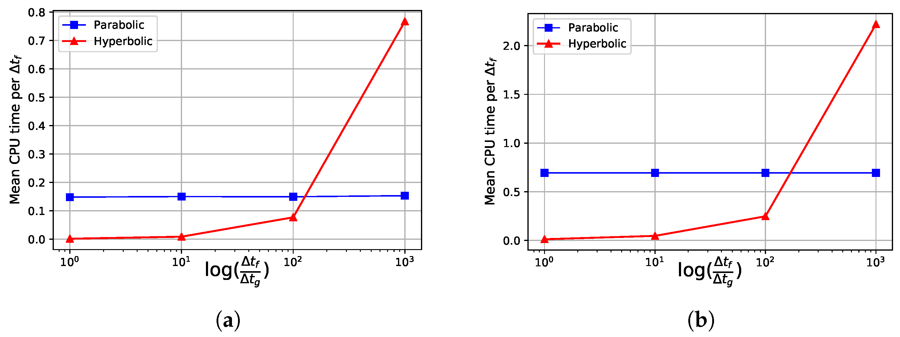
5.2.1. Study of the Critical Time Step Ratio Preserving the Performance of the Hyperbolic Grid Motion Solver

The first key topic of assessing regarding the computational relevance of the proposed hyperbolic solver of the grid motion problem is the critical time step ratio with the physical fluid problem, above which the original parabolic harmonic problem is less time-consuming.

This is independent of the considered fluid problem. The respective time steps for the physical problem set the steps when the harmonic grid problem is solved, and the hyperbolic problem parameters need to be chosen in the same stability domain, so that forced ratios between them are studied, with values 1, 10, 100 and 1000. Results are given in Figure 15 for the most refined mesh. Time is measured in terms of average time associated with the grid motion computational task per physical time step, labeled Mean CPU time per $\Delta t_f$ on the plots.

The critical time step ratio for the hyperbolic approach increases with the problem’s size and starts around 150 for the coarsest mesh to obtains close to 200 for the most refined one. This increase is related to the different evolution of the computational cost of the grid solver along with the mesh size for parabolic and hyperbolic approaches (see next section) and is likely to continue for bigger meshes, to the advantage of the hyperbolic grid motion. Given the ratios’ values in Table 2, the chosen fluid problem seems detrimental to the proposed approach. Only the soft grid appears competitive with the harmonic equation for the considered meshes. It is, however, only the consequence of the favored simplicity of the current test case, implementing, in particular, no initial flow or turbulence modeling. For instance, with an additional imposed flow at the average velocity of 2 m·s${}^{-1}$, the time step ratio resulting from the CFL condition would instead be given by the ratio between the speed of the sound in the grid problem and the average velocity in the physical fluid problem. In the proposed geometry, this would produce a ratio of 16 for the soft grid and 158 for the stiff grid, improving the competitiveness of the hyperbolic approach. Increasing the flow velocity to 5 m·s${}^{-1}$, thus entering the turbulent regime in the proposed geometry, and adding a transient turbulence model such as Large Eddy Simulation (see [35] among numerous references) would remain within very classical problems in the field of CFD simulation. It would further enhance the interest for the hyperbolic equation to solve the grid problem, with time step ratios going down to around 6 and 63 for the soft and stiff grids, respectively. The time step ratio is finally likely to go down to 1 and below if the proposed approach were to be applied to compressible flows, for which the parabolic harmonic equation then appears very penalizing for the ALE grid motion. The statements above are summarized in

Table 3. Competitiveness of the hyperbolic grid motion with respect to harmonic grid motion depending on the main features of various ALE problems in the proposed geometry.

Problem features	Simple laminar problem, fluid initially at rest	Low velocity initial flow (around 1 or 2 m·s${}^{-1}$), laminar regime	Higher velocity initial flow (>5 m·s${}^{-1}$), turbulent regime	Extension to compressible fluid models
Characteristic time step ratio	40 to 500 and more	15 to 300	5 to 60	Down to 1 or below
Competitiveness of hyperbolic equation	Critical (relevant for soft grid parameter, better with bigger meshes however)	Improved (for a wider range of grid parameters)	Strong	Crucial

.

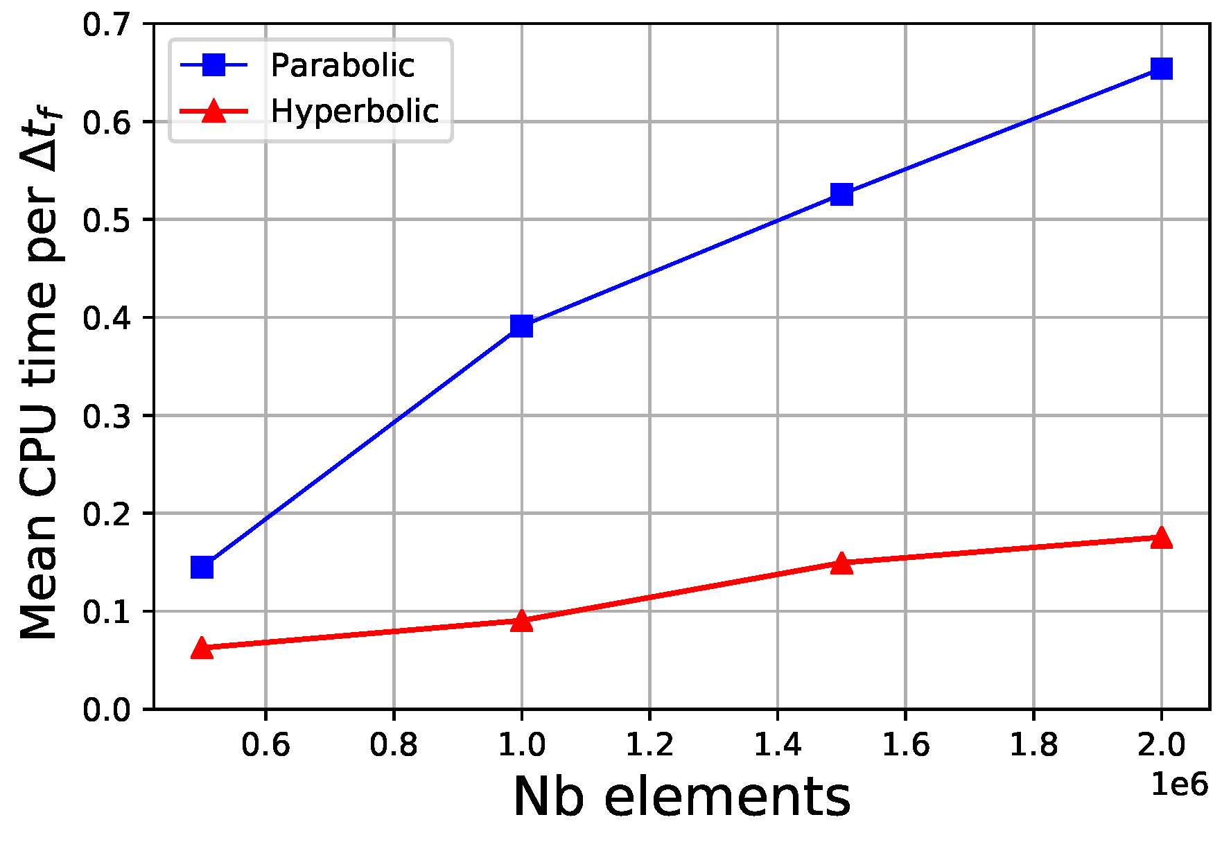
5.2.2. Evolution of the Computational Cost of the Grid Solver with the Mesh Size

Figure 16 provides a simple comparison of the evolution with the mesh size of the computational time needed to update the grid. Time is measured in the same manner as in the previous section. Although being established in the critical domain for competitiveness in terms of CFD features (see Table 3), this plot shows a significant advantage for the hyperbolic equation with soft grid parameters compared to the harmonic reference equation. The slope is already four times lower with the hyperbolic equation, and the evolution is likely to remain linear for bigger meshes due to only simple matrix-vector operations to perform. On the contrary, the evolution for the harmonic equation involving the solution of a linear system can be expected to be above linear, potentially increasing the gap in favor of the hyperbolic equation.

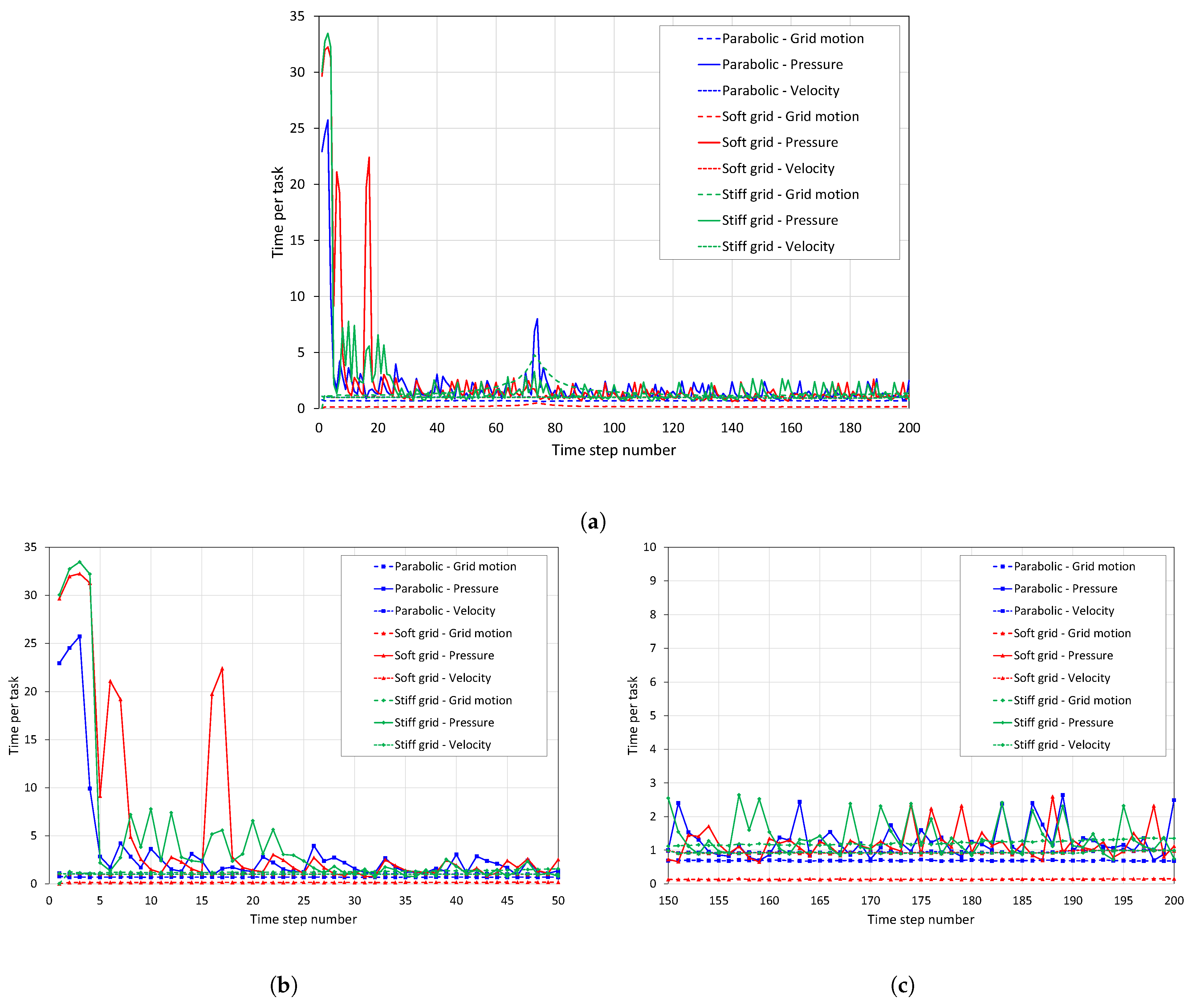
5.2.3. Study of Total Computation Time

The total computation time is analyzed based on a run with the most refined mesh and 200 time steps for a final time of $0.0576$ s. It corresponds to approximately half a period of the cylinder’s oscillation and is sufficient to obtain stable and reliable average costs per computational task involved in the resolution.

Figure 17 gives the evolution for each time step of the costs of the three main tasks, namely the evaluation of the displacements of all the grid points, named Grid Motion, the solution of the pressure problem ensuring the incompressibility of the fluid, named Pressure, and the implicit solution of the velocity problem, named Velocity. The plot for the sequence of 200 time steps yields three main observations:

• the costs for tasks Grid motion and Velocity are very stable,
• the most important cost is related to the Pressure task, and it exhibits some oscillations during the initial steps; this can be attributed to the velocity discontinuity at the initial step of the calculation,
• a stabilized regime is achieved after a certain number of steps (around 30).

Figure 17a exhibits a singular short peak around 75 time steps, but it is difficult to characterize since it involves the Pressure task with the parabolic grid motion only and to a lesser extent the Grid Motion task for the stiff grid only. This particular behavior would require extensive analysis and does not modify the main conclusions drawn in the following so that it is decided to focus on the other main aspects of the plot, shown in Figure 17b,c.

Regarding the initial phase in Figure 17b, the higher cost for the Pressure task at the beginning of the simulation comes from an increased number of iterations to reach convergence for the PCG algorithm, mainly due to the initial velocity jump to be accommodated by the pressure solver ensuring the incompressibility of the fluid. The hyperbolic equation for the grid problem amplifies this phenomenon, adding to the physical discontinuity a transient phase in the grid motion needed to propagate the discontinuous velocity from the boundary to the entire mesh. During this phase, the quality of the cells near the boundary can be degraded, and with it the conditioning of the matrix of the pressure system, resulting again in an increase in the number of iterations needed for the convergence of the PCG algorithm. The duration of the initial transient phase in terms of computational costs is logically all the more critical as the grid is soft.

Table 4. Computational times per time step in s and percentage of the total time for the different tasks.

	Harmonic Grid		Soft Grid		Stiff Grid
	With initial transient	Stabilized regime only	With initial transient	Stabilized regime only	With initial transient	Stabilized regime only
Grid Motion	$0.69$  $\left(\mathbf{19}\mathbf{\%}\right)$	$0.69$  $\left(\mathbf{23}\mathbf{\%}\right)$	$0.17$  $\left(\mathbf{5}\mathbf{\%}\right)$	$0.14$  $\left(\mathbf{6}\mathbf{\%}\right)$	$1.50$  $\left(\mathbf{32}\mathbf{\%}\right)$	$1.23$ $\left(\mathbf{35}\mathbf{\%}\right)$)
Pressure	$1.96$  $\left(\mathbf{54}\mathbf{\%}\right)$	$1.30$  $\left(\mathbf{44}\mathbf{\%}\right)$	$2.39$  $\left(\mathbf{68}\mathbf{\%}\right)$	$1.20$  $\left(\mathbf{52}\mathbf{\%}\right)$	$2.21$  $\left(\mathbf{47}\mathbf{\%}\right)$	$1.29$  $\left(\mathbf{27}\mathbf{\%}\right)$
Velocity	$0.98$  $\left(\mathbf{27}\mathbf{\%}\right)$	$0.97$  $\left(\mathbf{33}\mathbf{\%}\right)$	$0.98$  $\left(\mathbf{28}\mathbf{\%}\right)$	$0.97$  $\left(\mathbf{42}\mathbf{\%}\right)$	$0.98$  $\left(\mathbf{21}\mathbf{\%}\right)$	$0.96$  $\left(\mathbf{28}\mathbf{\%}\right)$
Total	$3.63$	$2.96$	$3.53$	$2.30$	$4.68$	$3.48$

gathers the average times per time step for the three computational tasks introduced above and the total time. Results differ slightly whether the initial transient phase is taken into account or not. Given the stability of the computational costs after the first 50 steps (except for the singular artifact seen around 75 steps affecting the various approaches differently), it appears legitimate to focus preferably on the stabilized regime to discuss the performance of the hyperbolic approach compared to the parabolic harmonic reference.

As expected, given the time step ratios between the fluid problem and the hyperbolic grid problem for the soft and stiff grids, respectively, only the former is competitive for the proposed test case. It then effectively cancels the cost of the grid motion while preserving the costs of the other computational tasks. The variation in the cost of the Pressure task in this case compared to the case with the harmonic grid motion is insignificant and results only from the residual oscillations in the convergence of the PCG algorithm for the Pressure task seen in Figure 17c.

However, the effect of the strategy implemented for the grid motion on the cost of the Pressure computational task, seen in the initial transient phase in Figure 17b, was not expected at this level. This has limited consequences in the present situation, and this effect will vanish for more extended simulations when the stabilized regime is preserved. It should be kept in mind and watched for problems that may exhibit other velocity discontinuities, for instance, from the structural behavior in fluid–structure interaction. This topic disappears if compressible flows are considered instead of an incompressible flow requesting an implicit solver for Pressure.

6. Recommended Strategy for the Optimal Choice of Parameters Introduced by the Hyperbolic Grid Motion

It is noteworthy that the new set of parameters introduced by the hyperbolic grid motion approach requests a prior appropriation and learning phase from the end-users to achieve optimal computational performance. This is a one-time investment that does not, in the general case, compete with the global efficiency of the approach. The relevant clues are provided in Section 3, Section 4 and Section 5, and once some optimal values are obtained for one problem, they are likely to serve as efficient default parameters for many cases in the same range of physics. In addition, over time, some understanding will be acquired about the grid’s response as a dynamic structural system, accelerating the calibration steps for new cases out of the range of already performed simulations.

It is pertinent to leverage the two significant observations made in the previous sections to initiate the appropriation process. However, the overall objective should be to determine fictitious material parameters that maximize grid stability while maintaining physical solution quality, namely, the fluid cell shape:

• Section 3.3 and Section 5.2.3 show that the quality of the mass and stiffness parameters is related to the motion of the structural boundaries, including both amplitude and velocity,
• Figure 16 shows that the efficiency of the hyperbolic approach for the grid motion increases with mesh refinement.

It is, therefore, strongly advised to conduct the first optimization of the fictitious parameters on a coarse version of the problem of interest. It will run quickly and likely exhibit sufficiently representative features in terms of structural motion to produce a robust set of mass and stiffness parameters. The performance in the last case will only be better than the one for the preliminary test.

Finally, it is reminded that tuning the fictitious damping is the way to kill any unwanted oscillation of the grid resulting from artificial wave propagation and that it has no influence on the stability thanks, to the formulation provided in Section 2.8.

7. Conclusions

This work introduces a new computationally efficient method for computing fluid grid motion from moving boundary conditions. Second-order time derivatives are used to transform the initial parabolic equation into a hyperbolic equation. The grid equation is resolved by employing an explicitly time-integrated scheme without addressing any additional large linear system. The respective influence of the fictitious grid parameters introduced with the hyperbolic equation, along with the global robustness of the proposed approach, are analyzed in detail with two dedicated small-size test cases. The new method’s performance concerning the parabolic reference approach for the grid motion is finally extensively studied through a last three-dimensional test case of significant size. The proposed strategy is practically able, with the right choice of parameters, to efficiently reduce and almost cancel the computational cost of updating the ALE fluid grid. The benefits are visible even for a test case whose chosen simplicity is placed in the critical domain for the competitiveness of the hyperbolic grid problem.

Considering that the merits of the hyperbolic model for the grid motion in ALE simulation are demonstrated in the current paper, the prospect for continuing this work is to address the related topic of the robustness of the grid motion in response to large boundary displacements. The basic process is to change the reference parabolic equation for more advanced models available in the literature and then transform it into another hyperbolic problem following the same steps as in the present article. Among the candidates for the following parabolic models, two, in particular, show great potential. On the one hand, the biharmonic equation [19] can significantly enhance the preservation of the shapes of the grid cells for large displacements, especially close to the moving boundary. It comes, however, with the need for quadratic finite element approximation within the grid problem solver, making it more complex to implement. Such a discretization is, for instance, currently unavailable with TrioCFD software (version 1.8.4, CEA, Saclay, France). On the other hand, replacing the harmonic equation with a mechanical problem introducing an entirely fictitious material better accounting for shear stress is also likely to enhance the robustness of the grid motion. If linear elastic materials are the first logical target, hyperelastic materials, such as Ogden material [36], should also be considered in a second step as a way to handle considerable grid deformation. Full mechanical models have the advantage of easy implementation with linear finite element approximation but also introduce additional parameters controlling the dynamics of the grid motion when converted into the hyperbolic framework, yielding the need for specific characterization in the same manner as performed in the present research.

References

1. Gerbeau, J.F.; Vidrascu, M.; Frey, P. Fluid–structure interaction in blood flows on geometries based on medical imaging. Comput. Struct. 2005, 83, 155–165. [Google Scholar] [CrossRef]
2. Formaggia, L.; Quarteroni, A.; Veneziani, A. (Eds.) Cardiovascular Mathematics: Modeling and Simulation of the Circulatory System; Number Volume 1 in Modeling, Simulation & Applications; Springer: Milan, Italy; Berlin/Heidelberg, Germany; New York, NY, USA, 2009. [Google Scholar]
3. Piperno, S.; Farhat, C. Partitioned procedures for the transient solution of coupled aeroelastic problems- Part II. Comput. Methods Appl. Mech. Eng. 2001, 190, 3147–3170. [Google Scholar] [CrossRef]
4. Lesoinne, M.; Farhat, C. Higher-Order Subiteration-Free Staggered Algorithm for Nonlinear Transient Aeroelastic Problems. AIAA J. 1998, 36, 1754–1757. [Google Scholar] [CrossRef]
5. Ricciardi, G. Fluid-structure interaction modelling of a PWR fuel assembly subjected to axial flow. J. Fluids Struct. 2016, 62, 156–171. [Google Scholar] [CrossRef]
6. Lagrange, R.; Piteau, P.; Delaune, X.; Antunes, J. Fluid-Elastic Coefficients in Single Phase Cross Flow: Dimensional Analysis, Direct and Indirect Experimental Methods. In Proceedings of the Volume 4: Fluid-Structure Interaction, San Antonio, TX, USA, 14–19 July 2019. [Google Scholar]
7. Lu, D.; Liu, A.; Shang, C.; Dang, J.; Hong, Y.; Xie, Q. Experimental investigation on fluid–structure-coupled dynamic characteristics of the double fuel assemblies in a fast reactor. Nucl. Eng. Des. 2013, 255, 180–184. [Google Scholar] [CrossRef]
8. Degroote, J. Partitioned simulation of fluid-structure interaction. Arch. Comput. Methods Eng. 2013, 20, 185–238. [Google Scholar] [CrossRef]
9. Fernández, M.A. Coupling schemes for incompressible fluid-structure interaction: Implicit, semi-implicit and explicit. SeMA J. 2011, 55, 59–108. [Google Scholar] [CrossRef]
10. Zhang, Q.; Hisada, T. Studies of the strong coupling and weak coupling methods in FSI analysis. Int. J. Numer. Methods Eng. 2004, 60, 2013–2029. [Google Scholar] [CrossRef]
11. Puscas, M.A.; Monasse, L. A three-dimensional conservative coupling method between an inviscid compressible flow and a moving rigid solid. SIAM J. Sci. Comput. 2015, 37, B884–B909. [Google Scholar] [CrossRef]
12. Monasse, L.; Daru, V.; Mariotti, C.; Piperno, S.; Tenaud, C. A conservative coupling algorithm between a compressible flow and a rigid body using an embedded boundary method. J. Comput. Phys. 2012, 231, 2977–2994. [Google Scholar] [CrossRef]
13. Puscas, M.A.; Monasse, L.; Ern, A.; Tenaud, C.; Mariotti, C. A conservative Embedded Boundary method for an inviscid compressible flow coupled with a fragmenting structure. Int. J. Numer. Methods Eng. 2015, 103, 970–995. [Google Scholar] [CrossRef]
14. Puscas, M.A.; Monasse, L.; Ern, A.; Tenaud, C.; Mariotti, C.; Daru, V. A time semi-implicit scheme for the energy-balanced coupling of a shocked fluid flow with a deformable structure. J. Comput. Phys. 2015, 296, 241–262. [Google Scholar] [CrossRef]
15. Donea, J.; Huerta, A.; Ponthot, J.P.; Rodríguez-Ferran, A. Arbitrary Lagrangian-Eulerian Methods. In Encyclopedia of Computational Mechanics; John Wiley & Sons, Inc.: Hoboken, NJ, USA, 2004. [Google Scholar]
16. Helenbrook, B.T. Mesh deformation using the biharmonic operator. Int. J. Numer. Methods Eng. 2003, 56, 1007–1021. [Google Scholar] [CrossRef]
17. Dwight, R.P. Robust mesh deformation using the linear elasticity equations. In Computational Fluid Dynamics 2006; Springer: Berlin/Heidelberg, Germany, 2009; pp. 401–406. [Google Scholar]
18. Faucher, V.; Bulik, M.; Galon, P. Updated VOFIRE algorithm for fast fluid–structure transient dynamics with multi-component stiffened gas flows implementing anti-dissipation on unstructured grids. J. Fluids Struct. 2017, 74, 64–89. [Google Scholar] [CrossRef]
19. Wick, T. Fluid-structure interactions using different mesh motion techniques. Comput. Struct. 2011, 89, 1456–1467. [Google Scholar] [CrossRef]
20. Stein, K.; Tezduyar, T.; Benney, R. Mesh Moving Techniques for Fluid-Structure Interactions With Large Displacements. J. Appl. Mech. 2003, 70, 58–63. [Google Scholar] [CrossRef]
21. Yigit, S.; Schäfer, M.; Heck, M. Grid movement techniques and their influence on laminar fluid–structure interaction computations. J. Fluids Struct. 2008, 24, 819–832. [Google Scholar] [CrossRef]
22. Angeli, P.E.; Bieder, U.; Fauchet, G. Overview of the TrioCFD code: Main features, V&V procedures and typical applications to nuclear engineering. In Proceedings of the 16th International Topical Meeting on Nuclear Reactor Thermal Hydraulics (NURETH-16), Chicago, IL, USA, 30 August–4 September 2015. [Google Scholar]
23. Angeli, P.E.; Puscas, M.A.; Fauchet, G.; Cartalade, A. FVCA8 benchmark for the Stokes and Navier-Stokes equations with the TrioCFD code—Benchmark session. In Proceedings of the Finite Volumes for Complex Applications VIII—Methods and Theoretical Aspects, Lille, France, 12–16 June 2017; pp. 181–202. [Google Scholar]
24. Bieder, U.; Rodio, M.G. Large Eddy Simulation of the injection of cold ECC water into the cold leg of a pressurized water reactor. Nucl. Eng. Des. 2019, 341, 186–197. [Google Scholar] [CrossRef]
25. Panunzio, D.; Puscas, M.A.; Lagrange, R. Vibrations of immersed cylinders. Simulations with the engineering open-source code TrioCFD. Test cases and experimental comparisons. C. R. Mécanique 2022, 350, 451–476. [Google Scholar] [CrossRef]
26. Nobile, F. Numerical Approximation of Fluid-Structure Interaction Problems with Application to Haemodynamics. Ph.D. Thesis, EPFL, Lausanne, Switzerland, 2001. [Google Scholar] [CrossRef]
27. Piperno, S. Simulation Numérique de Phénomènes d’Interaction Fluide-Structure. Ph.D. Thesis, École National des Ponts et Chaussées, Champs-sur-Marne, France, 1995. [Google Scholar]
28. Lohner, R.; Yang, C. Improved ALE mesh velocities for moving bodies. Commun. Numer. Methods Eng. 1996, 12, 599–608. [Google Scholar] [CrossRef]
29. Fiorini, C.; Després, B.; Puscas, M.A. Sensitivity equation method for the Navier-Stokes equations applied to uncertainty propagation. Int. J. Numer. Methods Fluids 2021, 93, 71–92. [Google Scholar] [CrossRef]
30. Guermond, J.L.; Minev, P.; Shen, J. An overview of projection methods for incompressible flows. Comput. Methods Appl. Mech. Eng. 2006, 195, 6011–6045. [Google Scholar] [CrossRef]
31. Temam, R. Une méthode d’approximation de la solution des équations de Navier-Stokes. Bull. Société Mathématique Fr. 1968, 96, 115–152. [Google Scholar] [CrossRef]
32. de Moura, C.A.; Kubrusly, C.S. The Courant–Friedrichs–Lewy (CFL) Condition. 80 Years after Its Discovery; Scientific Computation; Birkhäuser: Boston, MA, USA, 2013. [Google Scholar] [CrossRef]
33. Turek, S.; Hron, J.; Razzaq, M.; Wobker, H.; Schäfer, M. Numerical Benchmarking of Fluid-Structure Interaction: A Comparison of Different Discretization and Solution Approaches. In Fluid Structure Interaction II; Springer: Berlin/Heidelberg, Germany, 2010; pp. 413–424. [Google Scholar]
34. Razzaq, M.; Turek, S.; Hron, J.; Acker, J.; Weichert, F.; Grunwald, I.; Roth, C.; Wagner, M.; Romeike, B. Numerical simulation and benchmarking of fluid-structure interaction with application to hemodynamics. In Fundamental Trends in Fluid-Structure Interaction; World Scientific: Singapore, 2010; pp. 171–199. [Google Scholar]
35. Sagaut, P. Large Eddy Simulation for Incompressible Flows; Scientific Computation; Springer: Berlin/Heiderberg, Germany, 2006. [Google Scholar] [CrossRef]
36. Ogden, R.W. Large Deformation Isotropic Elasticity—On the Correlation of Theory and Experiment for Incompressible Rubberlike Solids. Proc. R. Soc. Lond. Ser. Math. Phys. Sci. 1972, 326, 565–584. [Google Scholar] [CrossRef]
Figure 1. Geometry for the pseudo-1D compression test case.
Fluids 08 00156 g001
Figure 2. Mesh motion in the first test case during a single period of 0.1 s. (a) Initial condition at t = 0 s. (b) Maximum compression of the domain at t = 0.05 s. (c) Return of the domain to the initial position t = 0.1 s.
Fluids 08 00156 g002
Figure 3. Evolution of the mesh velocity (in m·s 1 ) as a function of the damping coefficient d g . (Left): d g = 1 N·m·s 1 . (Right): d g = 10 5 N·m·s 1 . Time t = { 0.002 , 0.015 , 0.023 , 0.03 } s from top to bottom.
Fluids 08 00156 g003
Figure 4. Largest angle by element (in degrees) at maximum compression between several grids with different stiffness. The stiffness coefficient increases from the the left to the right. (a) Maximum compression; stiffness k g = 10 4 Pa. (b) Maximum compression; stiffness k g = 10 6 Pa. (c) Maximum compression; stiffness k g = 10 8 Pa.
Fluids 08 00156 g004
Figure 5. Largest angle by element (in degrees) at its return to the initial position ( t = 0.1 s) for different stiffness coefficients affected to the grid. The stiffness coefficient increases from the left and to the right. The last subpicture shows the initial grid mesh. (a) Return to the initial position; stiffness k g = 10 4 Pa. (b) Return to the initial position; stiffness k g = 10 6 Pa. (c) Return to the initial position; stiffness k g = 10 8 Pa. (d) Initial mesh.
Fluids 08 00156 g005
Figure 6. Largest angle by element (in degrees) at maximum compression between several grids with different density. The density increases between the left and right grid. (a) Maximum compression for grid ρ g = 10 3 kg·m 3 . (b) Maximum compression for grid ρ g = 10 4 kg·m 3 . (c) Maximum compression for grid ρ g = 10 5 kg·m 3 .
Fluids 08 00156 g006
Figure 7. Geometry for the Turek test case. (a) Zoom on the beam part. (b) The entire geometry of the domain.
Fluids 08 00156 g007
Figure 8. Turek test case with imposed displacement. Motion of the stiff grid. (a) Displacement of the beam at t = 0.025 s. (b) Displacement of the beam at t = 0.075 s.
Fluids 08 00156 g008
Figure 9. Evolution of the minimum of the Jacobian determinant, J, for the soft (left) and stiff (right) grids over three oscillation periods of the first bending mode of vibration of the clamped-free beam. The dashed lines correspond to the evolution of J for the harmonic grid.
Fluids 08 00156 g009
Figure 10. Evolution of the normalized minimum cells grid area for the soft (left) and stiff (right) grids over three oscillation periods of the first bending mode of vibration of the clamped-free beam. The dashed lines correspond to the evolution of J for the harmonic grid.
Fluids 08 00156 g010
Figure 11. Evolution of the minimum of the Jacobian determinant, J, for the soft (left) and stiff (right) grids over three oscillation periods of the bending mode of vibration of the clamped-free beam. The dashed lines correspond to the evolution of J for the harmonic grid.
Fluids 08 00156 g011
Figure 12. Evolution of the normalized minimum cells grid area for the soft (left) and stiff (right) grids over three oscillation periods. The dashed lines correspond to the evolution of J of the harmonic grid.
Fluids 08 00156 g012
Figure 13. Geometry for the 3D test case.
Fluids 08 00156 g013
Figure 14. Motion of the pinned-pinned inner cylinder. (a) Beam at its maximum compression upward at t = 0.025 s (mesh velocity in m·s 1 ). (b) Beam at its maximum compression downward at t = 0.075 s (mesh velocity in m·s 1 ).
Fluids 08 00156 g014
Figure 15. Evolution of the average time (in s) per fluid time step needed to solve the grid motion with respect to the time step ratio between the physical problem and the hyperbolic problem. The reference time associated to the parabolic harmonic equation is obviously independent from the ratio. (a) Results for the coarsest mesh 1. (b) Results for the most refined mesh 4.
Fluids 08 00156 g015
Figure 16. Evolution of the average time (in s) needed to solve the grid motion along with the mesh size.
Fluids 08 00156 g016
Figure 17. Evolution of the average computational times (in s) per main task and per time step during the simulation. (a) Results for the full sequence of 200 time steps; (b) Results for the first 50 time steps (i.e., initial transient). (c) Results for the last 50 time steps (i.e., stabilized regime).
Fluids 08 00156 g017