1. Introduction
A common problem in streamflow records from different regions around the world is the presence of gaps in the data that limit their usefulness for hydrological modeling, water resources management, and engineering applications [
1,
2]. Various factors can lead to missing discharge values in long-term flow-discharge datasets such as faulty or broken monitoring equipment, harsh weather conditions that affect the measurements, difficulty in accessing the measurement sites due to terrain or security issues, accidental absence of observers who collect the data, errors caused by human mistakes or negligence, budget limitations that constrain the data-collection and maintenance activities, and social or political unrest that disrupts normal operations. These factors can result in missing discharge values in long-term flow-discharge datasets [
2,
3]. This can result in information loss or misinterpretation of historical flow-regime changes and hydrological processes [
3,
4].
The reconstruction of historical streamflow data plays a vital role in water resource management, providing information about past water supplies [
5]. This knowledge is critical for comprehending the long-term variability of streamflow, which is necessary for sustainable water management. Historical streamflow data can also be used to evaluate the impact of human activities, such as the construction of dams and water usage, on water resources. Moreover, incorporating historical streamflow data into hydrological models can improve the accuracy of predicting future streamflow patterns and water availability [
6,
7,
8]. Therefore, accurately predicting the missing discharge values is crucial for dependable water resource management at the basin level.
Forecasting and backcasting the streamflow in the medium to long term is a complex task, owing to several factors such as human activities, changes in climate, and geographic characteristics. This complexity can be further compounded when dealing with streamflow data from gauges over a vast area, as the data may be sourced from rivers with regulated and unregulated flow patterns. Consequently, filling in data gaps can be challenging [
2,
6,
9].
Over the past few years, there has been a notable increase in research focused on streamflow reconstruction, with numerous scholars contributing to a more comprehensive understanding of this field. The utilization of a diverse range of methods and techniques by these researchers has resulted in a wealth of knowledge and insights into the intricate patterns and fluctuations of streamflow, as highlighted by recent studies [
10,
11,
12]. In a recent study by Thanh et al. [
3], six different machine-learning models were employed to reconstruct the daily average discharge in the Mekong River Basin and the Vietnamese Mekong Delta from 1980 to 2015. The models included the random forest regressor, Gaussian process regression, support vector regression, decision tree, least squares support vector machine, and multivariate adaptive regression spline. The accuracy of each model was evaluated by comparing it to stage-discharge rating curves. According to the authors, the decision tree model was not recommended for their region of interest. However, they reported that the Gaussian process regression and support vector regression models produced acceptable results. Arriagada et al. [
12] used the missforest method to address gaps in daily streamflow time series in a region with significant climatic variability. Unlike the random forest regression (RFR) method, missforest approached the problem of missing data as a prediction problem. The results indicated that the reconstructed daily streamflow time series of rivers with natural flow patterns were accurately simulated, though the performance was slightly lower for rivers affected by urban runoff and water diversion for irrigation. However, in cases of significant changes to the flow regime, such as hydropeaking, missforest was not successful in filling gaps in the daily streamflow series. The reconstructed hydrographs offer valuable information about the variability and changes in streamflow and their relationship with important climatic variables. In a study by Xu et al. [
11], a deep learning model called CNN-GRU was tested on various watersheds globally. The findings indicated that the model performed better in making monthly streamflow predictions in watersheds with large drainage areas (over 3000 km
2). The performance of the model improved as the training period was extended, with a training period of 25–35 years being adequate for the majority of watersheds.
Several studies have focused on developing predictive models for multiscale variables-driven streamflow modeling. One such study by Sun et al. [
13] proposed a framework that aimed to enhance runoff forecasting accuracy and support decision making. This framework, named RF-GPR-MV, utilized random forest (RF) and Gaussian process regression (GPR) integrated with multiscale variables, including hydrometeorological and climate predictors, as inputs. The RF component of the MVDSF framework improved forecasting performance, contributing an average of around 25%, with greater improvements observed for lead times exceeding three months. Szczepanek [
14] made a significant contribution by comparing the performance of three gradient-boosting models (XGBoost, LightGBM, and CatBoost) in forecasting daily streamflow in a mountainous catchment. The study utilized daily precipitation, upstream gauge station runoff, and two-day preceding observations as predictors, with a minimum of 12 years of training data required to achieve desirable results. Surprisingly, XGBoost, which is the most popular model, did not yield the best performance. The study found that when using default model parameters, CatBoost achieved the best results. However, the optimization of hyperparameters led to LightGBM yielding the best predicted results. Several other studies have investigated multivariable streamflow forecasting [
15,
16,
17].
The Athabasca River Basin (ARB) has been a vital contributor to the economy of Alberta province since the advent of the oil and gas industry in 1967. In addition to the oil and gas sector, the region is home to other important economic activities such as agriculture, forestry, mining, and tourism [
18]. The majority of the ARB, which spans approximately 82% of its total land area, is covered by a dense boreal forest [
19]. Despite its significance, the ARB has undergone substantial changes in recent decades, primarily due to human activities. Urban expansion and industrial commodity production, including agriculture expansion, forest degradation, and coal and oil mining, have all played a crucial role in transforming the region. These activities have led to rapid alterations in the ARB’s landscape, which have been intensified by the presence of natural hazards such as wildfires [
18,
20].
In many studies, a thirty-year baseline period covering the years 1961 to 1990 has been utilized for a variety of analyses and calculations of anomalies [
21,
22,
23,
24]. The Intergovernmental Panel on Climate Change (IPCC) [
25] has recommended this thirty-year time frame as a standard that can encompass a diverse range of climate variations, including extreme droughts, floods, and fluctuations in temperature during different seasons. To ensure comprehensive modeling and extension of the streamflow time series, the inclusion of this baseline period was made within the considered time frame of January 1960 to December 2021.
In this article, a machine-learning framework is introduced that has the ability to predict missing or incomplete data in monthly streamflow records with high accuracy. The framework achieves this by utilizing historical data from various monthly streamflow datasets within the same region. The framework is designed to identify the most suitable gap-free monthly streamflow datasets from multiple possible combinations. The performance of the resulting models is evaluated using cross validation and the coefficient of determination. Through this process, the streamflow time series for all hydrometric stations in the study is extended with a high level of accuracy. The organization of the remainder of this article is as follows: the study region, datasets, and framework for the reconstruction of monthly streamflow, which involves the use of 12 ensemble machine-learning models, are outlined in
Section 2.
Section 3 presents the results of the framework, accuracy metrics, and correlation analyses. The findings are discussed in
Section 4, and the paper concludes in
Section 5.
2. Materials and Methods
2.1. Study Region
The Athabasca River Basin (ARB) covers roughly 160,000 km
2, which is nearly a quarter of Alberta’s province [
26]. It includes a number of named and unnamed rivers and lakes. With a length of 1538 km, the Athabasca River stands out as the largest natural river in the province of Alberta, having no obstructions such as dams. Moreover, the river’s drainage basin extends beyond 150,000 square kilometers, making it a crucial waterbody in the region [
27]. The region has both cold and warm seasons. During the cold months, a significant amount of precipitation comes in the form of snow, while during the warm months, meltwater and rainfall merge to contribute to river streamflow. Water from smaller basins also joins the main river as it flows towards Lake Athabasca [
19,
28]. The ARB region is depicted in
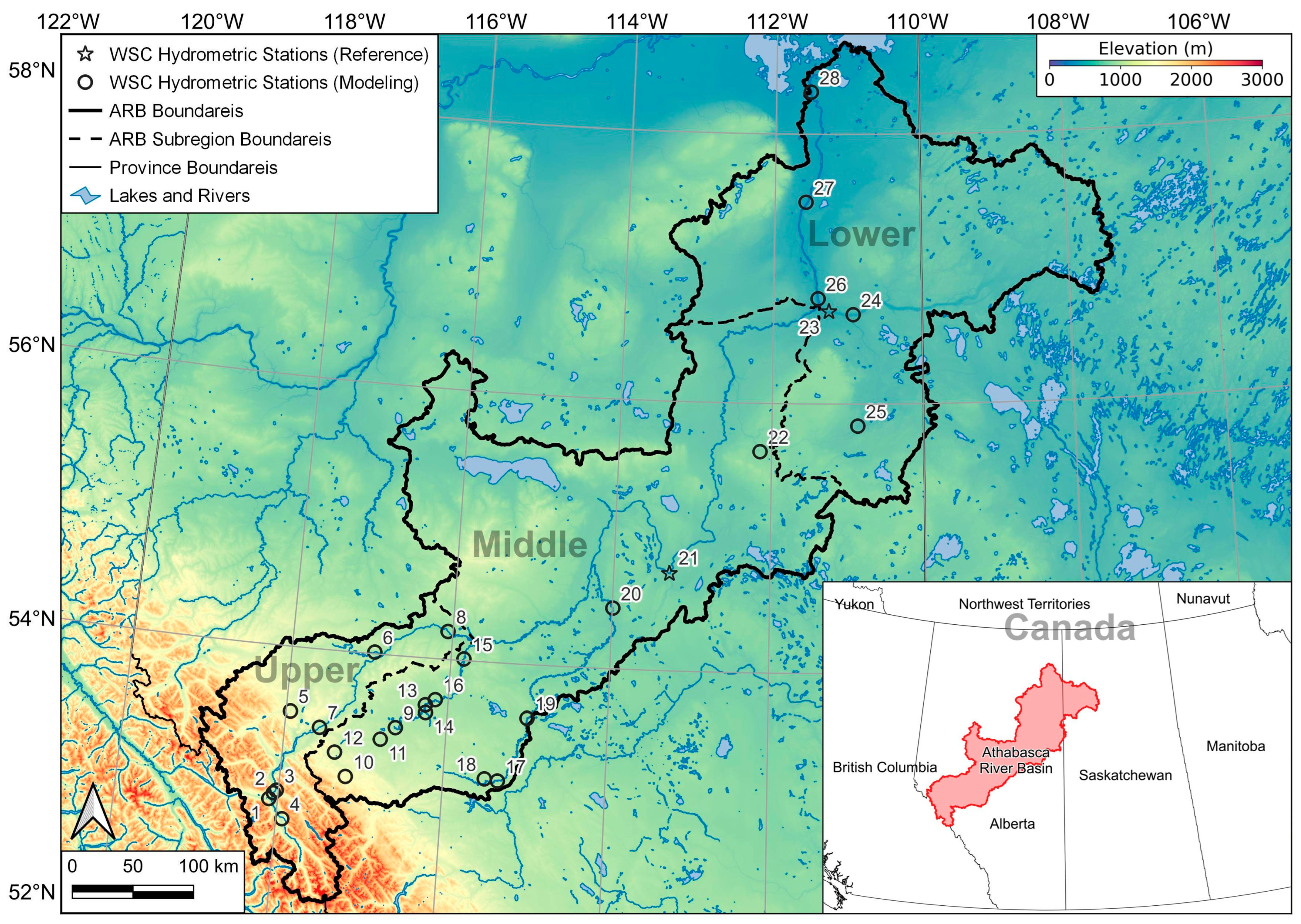
Figure 1, with the background gradient color generated using Shuttle Radar Topography Mission (SRTM) data sampled at 30 m. Based on varying climatic, hydrologic, and topographic traits, the ARB was classified into three hydro-physiographic areas, namely the lower ARB, middle ARB, and upper ARB [
29].
2.2. Streamflow Data
The streamflow data used in this study was acquired from the Water Survey of Canada (WSC) (
https://wateroffice.ec.gc.ca, accessed on 1 January 2023). The WSC collects concurrent hydrometric data, including streamflow and water level, from different hydrometric gauging stations across Canada. The hydrometric stations listed in
Table 1 were picked based on their record period, availability of continuous monthly streamflow data, the size of the drainage area (km
2), and their correlation with the rest of the stations selected in this study. The monthly streamflow time series for stations 07BE001 and 07CD001 were found to be continuous between January 1960 and December 2021 with no gaps and were used as the starting set for modeling the other monthly streamflow time series. WSC and the regional aquatics monitoring program (RAMP) (
http://www.ramp-alberta.org, accessed on 1 January 2023) data were fused for four stations (07CD005/S42, 07CE002/S29, 07DA041/S49, and 07DD001/S46) to eliminate minor gaps in the WSC data for these stations.
Figure 1 displays the geographical positions of these stations.
2.3. Methods
2.3.1. Modeling and Reconstructing Streamflow Time Series
Ensemble techniques are a way to enhance the performance of a predictive system by combining the predictions of multiple models. This is done through methods such as bagging, boosting, and stacking [
30]. A bagging method trains multiple models separately and combines their predictions by taking the average. A boosting method trains a sequence of models, with each model fixing the weaknesses of the previous model. A stacking method trains several models independently and then feeds their predictions into a higher- level model to make the final prediction [
30]. The random forest regressor (RFR), gradient boosting regressor (GBR), extra trees regressor (ETR), histogram-based gradient boosting regressor (HGBR), bagging regressor (BR), AdaBoost regressor (ABR) are some of the ensemble methods used for solving regression problems.
The RFR method involves the use of multiple decision-tree algorithms to generate predictions. It trains each tree on a separate part of the data, and the final prediction is made by taking the average of the predictions from all the trees in the forest. This method is effective for dealing with large amounts of data in high-dimensional spaces and is less susceptible to overfitting compared to a single decision tree [
31,
32].
The GBR is a regression method that employs the gradient-boosting algorithm, which combines weaker predictors, such as decision trees, to generate accurate predictions [
33,
34]. It continually improves the predictions by incorporating new decision trees that correct the errors of previous ones. GBR is acknowledged for its capacity to manage high-dimensional data, versatility, and resistance to overfitting, however, the training process of the model can be computationally intensive and take a considerable amount of time [
33,
34].
The ETR method builds an ensemble of decision trees, each of which is trained on a different part of the data. Unlike the random forest regressor, it chooses a random subset of features instead of considering all features when dividing a node. The final prediction is arrived at by taking the average of the predictions made by all the trees in the ensemble. This method can effectively handle large data sets in high-dimensional spaces and is less prone to overfitting than a standalone decision tree [
35,
36].
The HGBR is an adaptation of the gradient boosting regressor that uses histograms in place of traditional splitting methods. It generates more precise and flexible partitions by dividing the feature space into multiple bins through the use of histograms. HGBR can handle both categorical and continuous variables and is less impacted by the selection of hyperparameters, though the training process may be more demanding in terms of computational resources compared to the standard GBR [
35].
The BR is a method that utilizes multiple base models, each trained on a different part of the data, to make predictions. The final prediction is obtained by either averaging or taking a majority vote of the predictions from the base models. This technique helps to reduce the variance of complex models such as decision trees by introducing randomness in the training process and creating a combination of models [
35,
37].
The ABR is a technique for building a prediction model by training multiple versions of the same regressor, each time changing the weight of the instances based on the accuracy of the previous model. The final prediction is made by combining the predictions of all the regressors, with a focus on the instances that were more challenging to predict in the earlier models. This method helps to improve the accuracy of the model by iteratively adjusting the weight of the instances [
35,
38].
The split between the sizes of the training and testing sets is not predetermined and must be decided based on the amount of data available [
39]. For a small dataset, a larger proportion of the data should be designated for validation and testing, while for a larger dataset, a smaller proportion should be reserved for testing [
39]. To measure accuracy, the coefficient of determination (R
2) with 5-fold cross validation [
40] was utilized to evaluate the model’s performance on different portions of the data and detect any performance fluctuations. Each fold was divided into 70% for training and 30% for testing.
The optimal parameters were used to fine-tune the models, resulting in the creation of 12 models. The selection of the model with the highest accuracy on the test set was then performed. The development of the following 12 models took place at each step.
Random Forest Regressor (RFR);
Gradient Boosting Regressor (GBR);
Extra Trees Regressor (ETR);
Hist Gradient Boosting Regressor (HGBR);
RFR boosted with AdaBoost Regressor: RFR (ABR);
RFR boosted with Bagging Regressor: RFR (BR);
GBR boosted with AdaBoost Regressor: GBR (ABR);
GBR boosted with Bagging Regressor: GBR (BR);
ETR boosted with AdaBoost Regressor: ETR (ABR);
ETR boosted with Bagging Regressor: ETR (BR);
HGBR boosted with AdaBoost Regressor: HGBR (ABR);
HGBR boosted with Bagging Regressor: HGBR (BR).
Following a preliminary examination, it was discovered that the monthly streamflow data sets for 07BE001 and 07CD001 obtained from WSC had no gaps between January 1960 and December 2021. The list, including hydrometric stations 07BE001 and 07CD001, was referred to as the “non-gap list”, while the rest of the stations were in the “gap list”. The most correlated stations to 07BE001 and 07CD001 were identified through Pearson correlation, and initial modelings were performed using RFR for a streamflow time series from the gap list. A new round of modeling was initiated, whereby the station that exhibited the highest initial modeling score was chosen. For this station, a total of 12 models, as previously listed, were developed. Each of these 12 models underwent testing of all feasible feature combinations drawn from the nongap list. The model that achieved the highest test and train R2 scores was selected. The selected model was used to extend the available data to the full period of interest, and quality checks were conducted on the predicted values. If necessary, the number of features was adjusted based on Pearson correlation to improve the model’s performance. Once the model was deemed successful, the station was added to the nongap list and removed from the gap list. For every station in the gap list that remained, the procedure was repeated. In each iteration, the process started with the station having the best initial modeling score using the new nongap list.
A secondary iterative method was employed to improve the overall R
2 accuracy of the predictions. This involved using the original WSC/RAMP monthly streamflow time series, which had gaps, for the already extended time series that had the lowest R
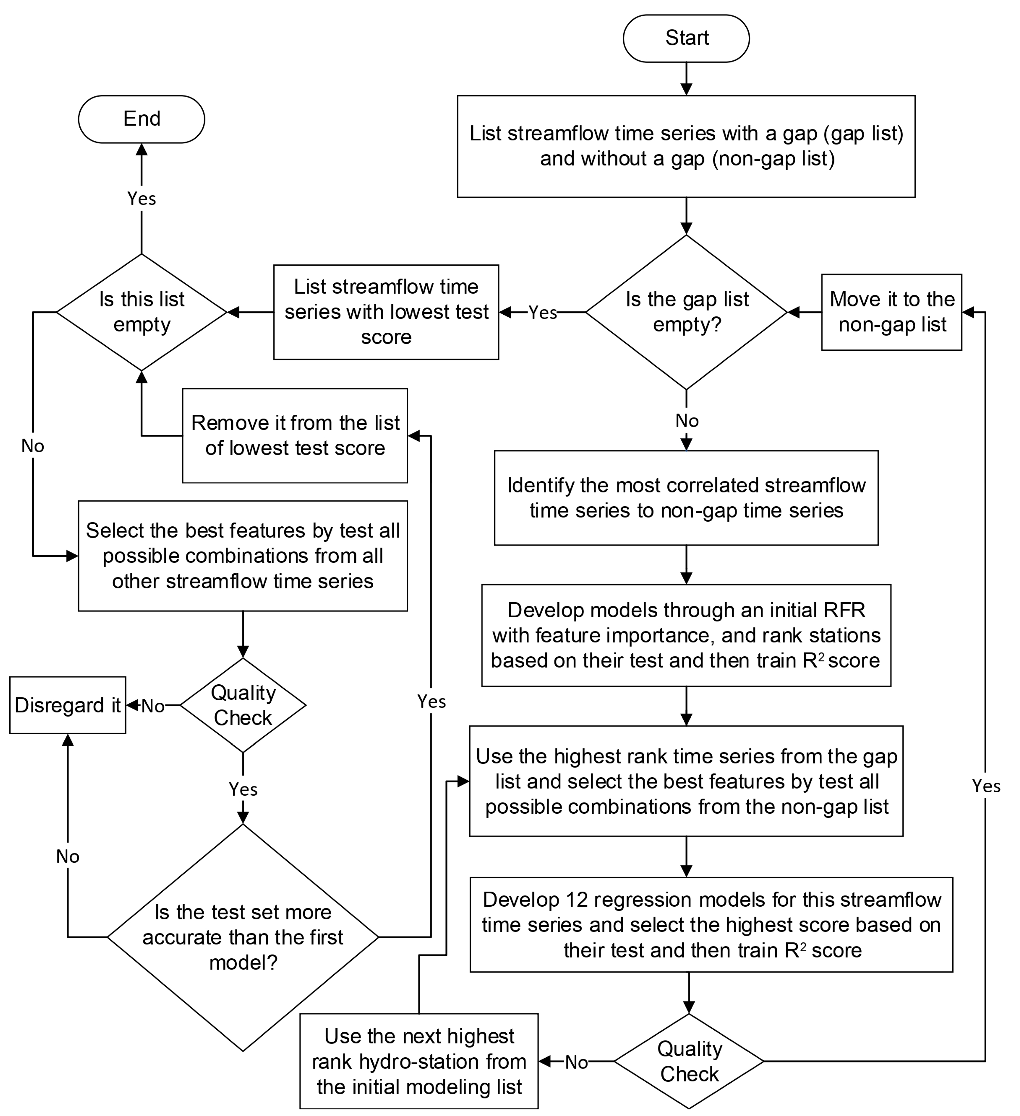
2 test score. This was done to enhance the level of modeling and precision of the predictions. If better accuracy metrics were achieved, quality control checks were conducted and, if satisfactory, the new extended time series replaced the previous one. The process of checking for improved results using the remaining 27 gap-free streamflow time series was repeated until no further improvements could be made. The workflow used for reconstructing each streamflow time series is illustrated in
Figure 2.
3. Results
3.1. Modeling and Reconstructing Streamflow Time Series
The historical monthly streamflow time series were reconstructed by following the procedure outlined in
Section 2.3.1 and in
Figure 2. Through this procedure, 26 streamflow time series were successfully reconstructed. R-squared (R
2) was used to assess the accuracy of the reconstructed streamflow time series.
The results of these metrics are summarized in
Table 2. The performance of each model was assessed using the coefficient of determination (R
2) and fivefold cross validation as the accuracy metric. The measured monthly streamflow data for each station was split into five train and test pairs, with each fold using 70% for training and 30% for testing. This process helped identify any fluctuations in the model’s performance. In
Table 2, the train and test scores are presented in the format of x.xx ±
, with the first component, x.xx, representing the mean of the R
2 scores obtained from the fivefolds, and the second component,
, reflecting the standard deviation of these scores. Additionally,
Table 2 presents the overall R
2 accuracy in its last column. This metric represents the R
2 score for all monthly streamflow data points that were measured and their corresponding predicted values across each streamflow time series and its associated predictive model.
The findings presented in
Table 2 indicate that GBR (BR) achieved the highest accuracy in seven out of the total instances, while ETR (BR) and GBR performed best in two cases. Among the seven GBR (BR) models, the overall R
2 score ranged from 0.9737 (for 07AG003) to 0.9968 (for 07AG007). The overall R
2 score for GBR models also had the lowest value of 0.9563 (for 07AA009) and the highest value of 0.9917 (for 07AA002). Additionally, the overall R
2 score for GBR models ranged from 0.9754 (for 07AC001) to 0.9911 (for 07AA002). The use of either BR or ABR improved the models, resulting in nearly 80% of the best models being based on these methods, with almost 73% of the models relying on gradient-boosted regression techniques such as GBR and HGBR.
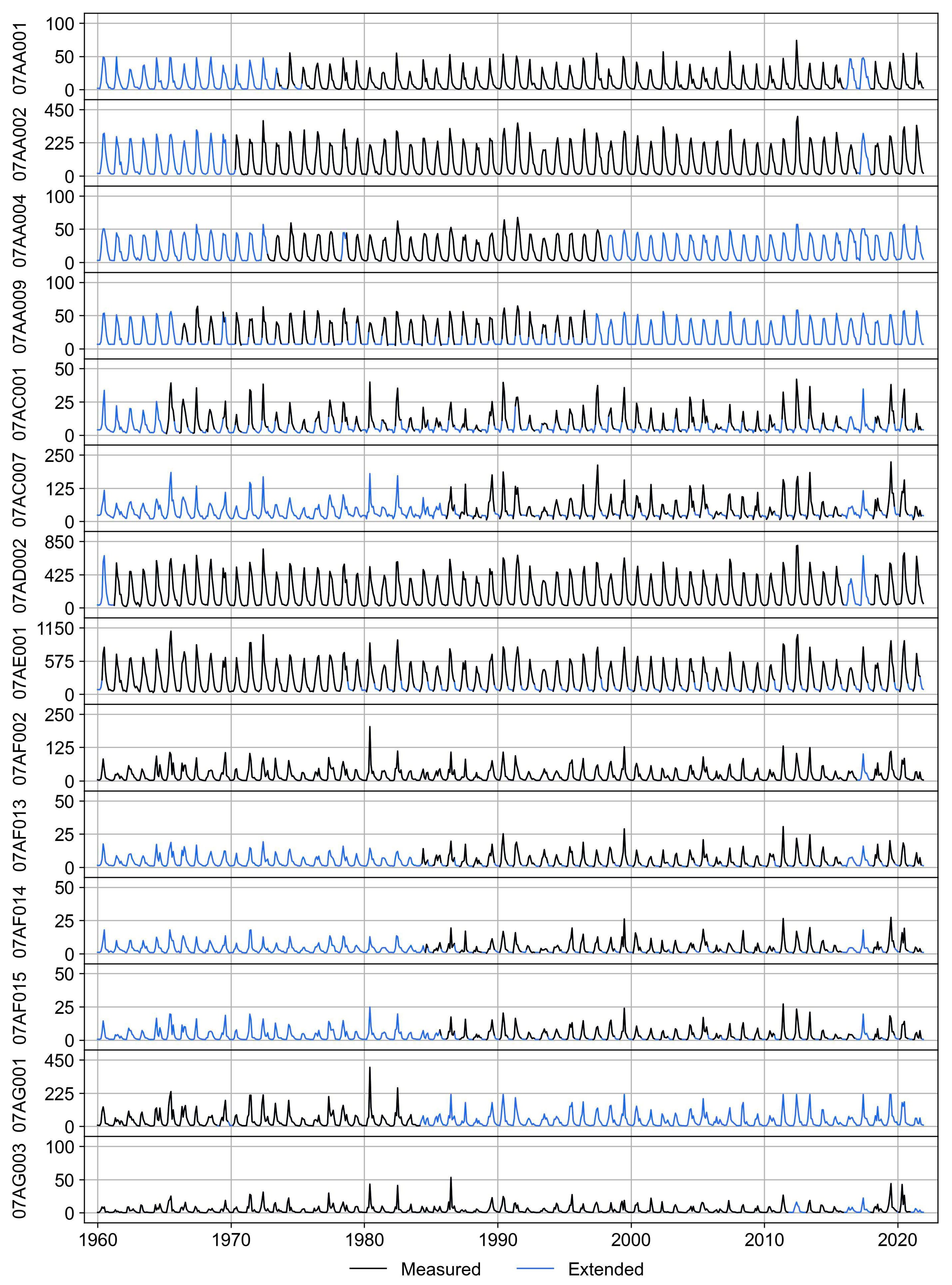
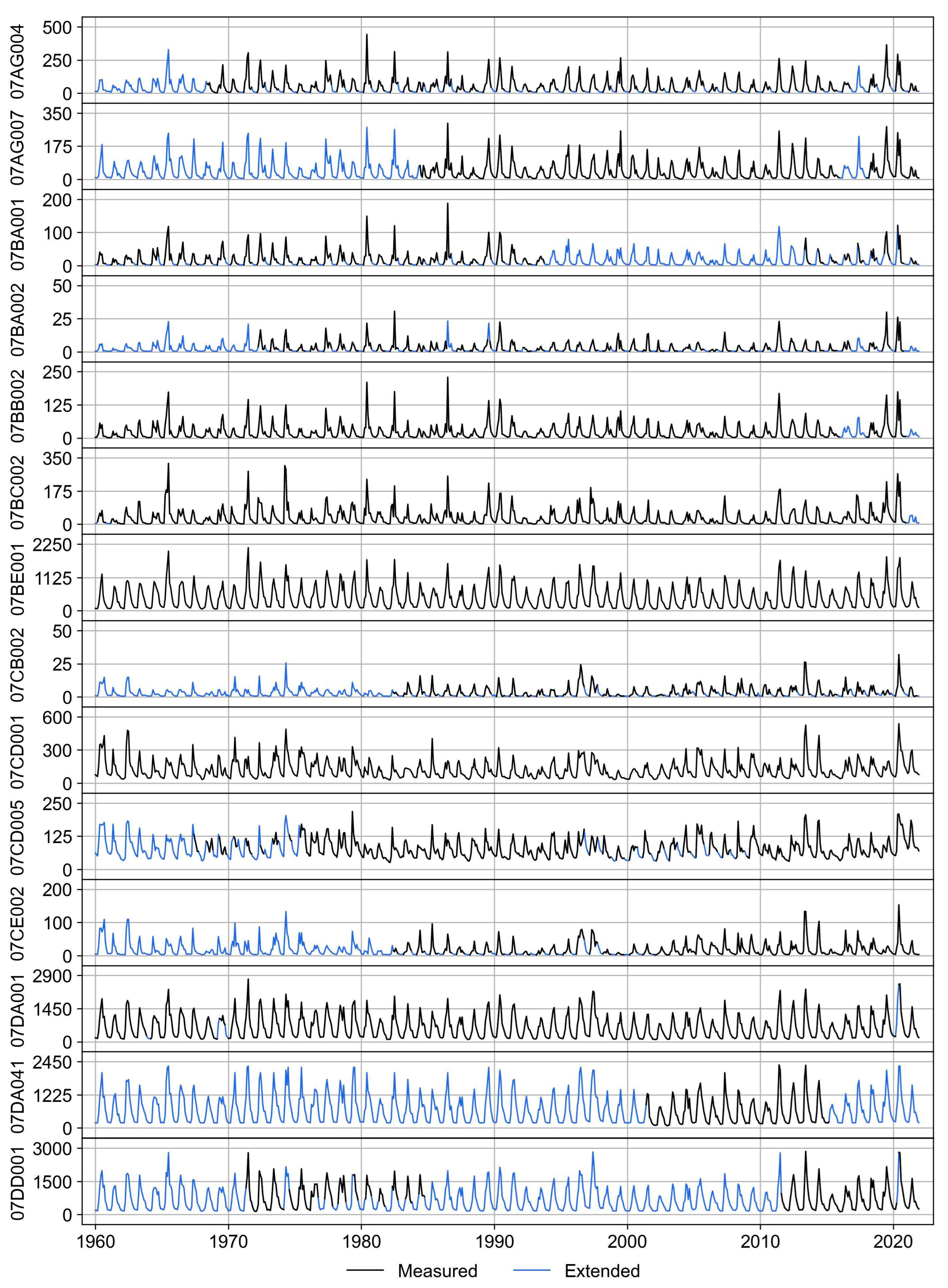
The monthly streamflow (m
3/s) time series, both measured and reconstructed, for each hydrometric station, are illustrated in
Figure 3 and
Figure 4. These figures provide a visual representation of reconstructed (extended) and measured monthly streamflow data. Sixteen of the 26 monthly streamflow time series contained more than 40% missing data during the period of interest. Notably, stations 07AF013, 07AG001, 07AF014, 07AF015, 07AC007, 07DD001, 07AA009, and 07DA041 had missing data exceeding 60% before the modeling process. Furthermore, stations 07DA001, 07DA041, and 07DD001 were positioned in the lower ARB region. Additionally, for each station,
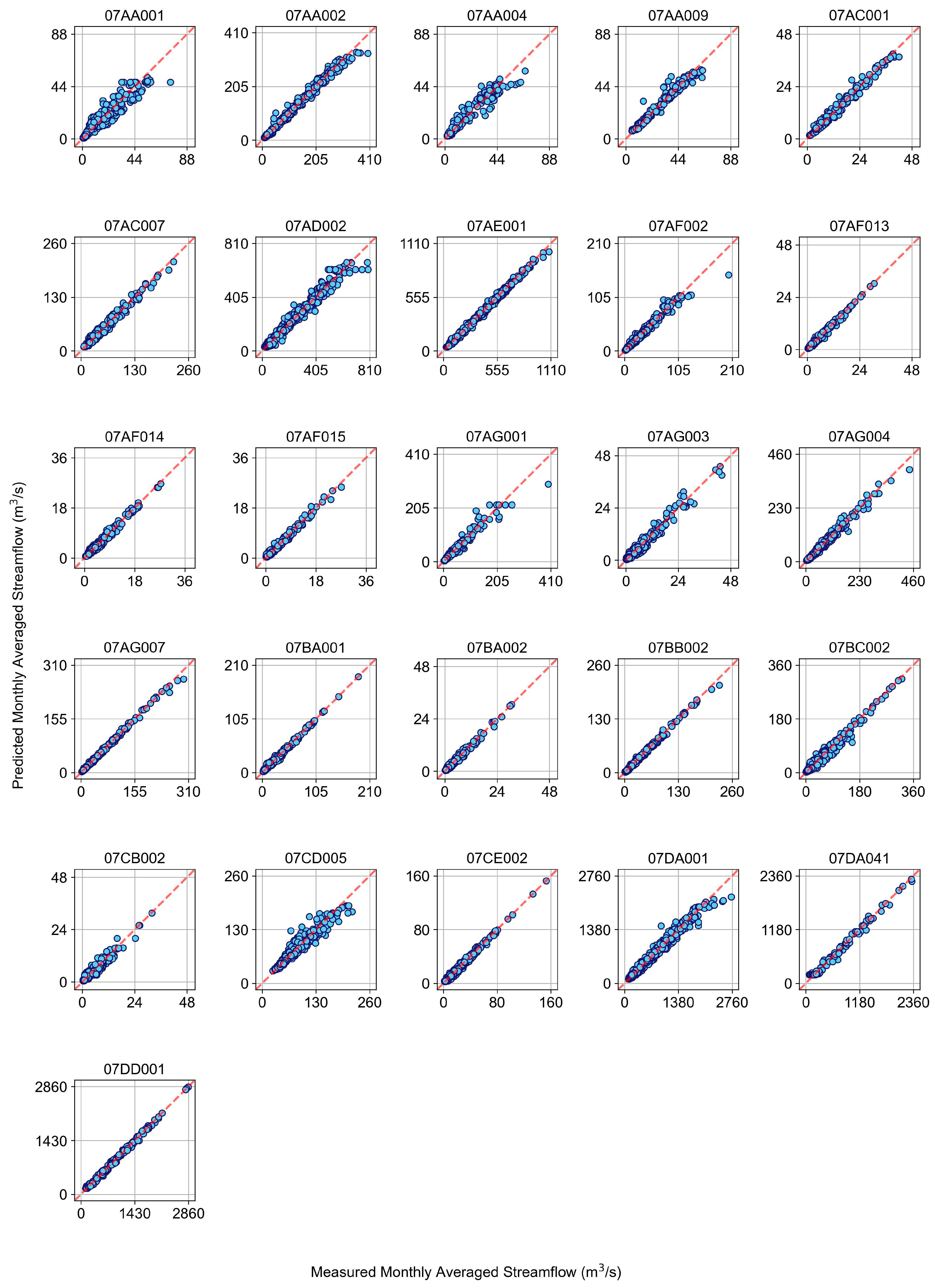
Figure 5 demonstrates the discrepancy between the predicted and measured monthly streamflow time series. The closeness of the blue dots to the red dashed line indicated the accuracy of the predictions, with the most accurate predictions located on the red dashed line. The accuracy of the predictions was measured using R
2 and displayed in the last column of
Table 2 and
Figure 5, indicating that the models with the highest overall R
2 scores also had more blue dots on or close to the red dashed line.
3.2. Analysis of Reconstructed Streamflow Time Series
A Pearson correlation estimates the linear association between two variables, denoted by the correlation coefficient, which ranges from −1 to 1. A positive correlation means that as one variable increases, the other variable also increases; a negative correlation means that as one variable increases, the other decreases. The magnitude of the correlation coefficient indicates the strength of the relationship, with values closer to 1 or −1 signifying a strong relationship, and values closer to 0 indicating a weak or no relationship [
41].
The extended monthly streamflow from
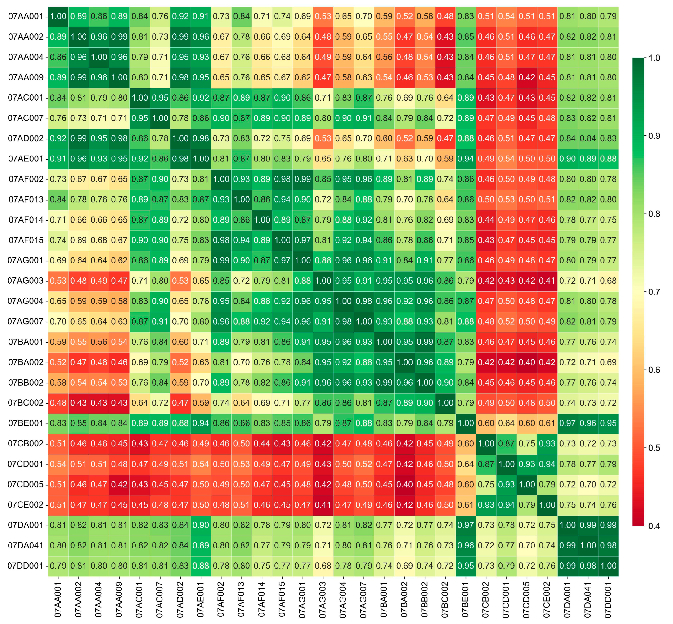
Section 3.1 was utilized to determine the most-correlated monthly streamflow time series. The Pearson correlation scores between 28 measured/extended monthly streamflow time series are displayed in
Figure 6. Accord- ing to
Figure 6, the minimum calculated correlation score between two distinct monthly streamflow time series was 0.40, and the top-five stations with the highest sum of Pearson correlations with the remaining stations were 07BE001, 07DA001, 07DA041, 07DD001, and 07AG007. These stations were all situated along the Athabasca River, the primary river in the ARB, except 07AG007 which was located along the McLeod River. Station 07BE001 was distinguished as a unique station in the ARB region due to its strong correlations (at least 0.60) with the other 27 stations analyzed. The station was located near the center of the ARB and was in close proximity to the Athabasca River.
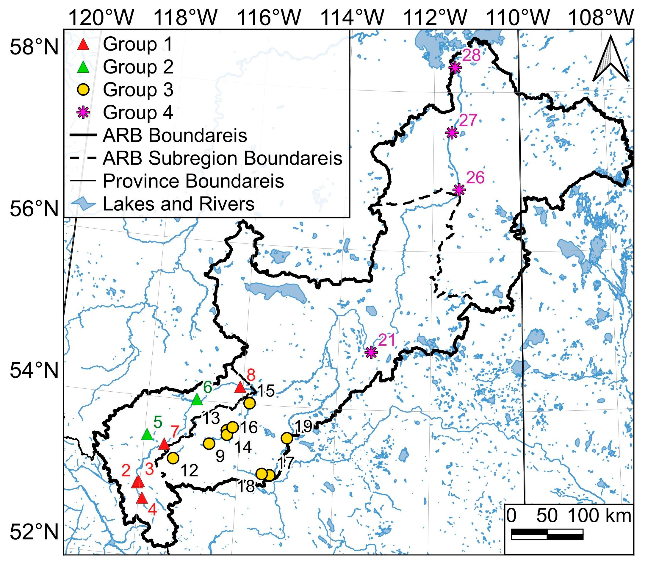
The map in
Figure 7 presents four groups of hydrometric stations, categorized based on their Pearson correlation of monthly streamflow. Group one contains five stations, 07AA002, 07AA004, 07AA009, 07AD002, and 07AE001, which were located in the vicinity of the Athabasca River and situated in the upper ARB region. Out of these, 07AA002, 07AA004, and 07AA009 had elevations in the range of 1000–1200 m, while 07AD002 had an elevation of 963 m and 07AE001 had an elevation of 735 m. Group two includes two stations, 07AC001 and 07AC007, which are located, respectively, on the northwest and north side of the upper ARB. Group three encompasses nine stations, 07AF002, 07AF015, 07AG001, 07AG003, 07AG004, 07AG007, 07BA001, 07BA002, and 07BB002. All were located in the middle ARB region. The stations 07BA001, 07BA002, and 07BB002 were situated along the Pembina River while the rest were located along the McLeod River. Group four includes three stations, 07BE001, 07DA001, and 07DA041, situated along the Athabasca River. Station 07BE001 was in the middle ARB, while the other two were in the lower part of the ARB.
4. Discussion
Our framework used for monthly streamflow reconstructions examined all possible combinations of gap-free historical data to choose the optimal model from 12 ensemble regression models to reconstruct monthly streamflow data for each station. Following this, the framework further refined the reconstructed streamflow time series by remodeling monthly streamflows for stations that had lower overall R2 scores. This iterative modeling was performed using the best models and feature combinations, provided there was room for improvement in the newly reconstructed streamflow time series. The task was challenging due to the complexity of the streamflow dynamics. The monthly streamflow for 07DA041 from January 2017 to December 2021 was very low (mostly less than 1 m3/s), which differed significantly from previous years’ records. This part of the 07DA041 dataset was treated as missing. The rest of the station data was used as it was available from the WSC website. On the other hand, the daily streamflow datasets for all stations were also acquired. In a few cases, minor differences were noted between the calculated monthly average through the daily streamflow data and the available monthly streamflow values. As the modelings were dependent on data quality, the monthly streamflow from WSC was utilized to ensure that any potential postprocessing done by the WSC data engineers was taken into consideration.
The monthly streamflow time series were reconstructed in this study following the procedure outlined in
Section 2.3. The accuracy of the reconstructed streamflow was assessed using the R
2 metric and fivefold cross validation. In general, stations that had higher Pearson correlations with other stations resulted in a higher R
2 accuracy on the test set for their best-performing model. Extreme sudden changes in some streamflow behavior resulted in lower accuracy for the models associated with these streamflows. For instance, 07AA001 showed a substantial discrepancy between the predicted (47.59 m
3/s) and measured (74.0 m
3/s) monthly streamflow values at one instance (June 2016). This large discrepancy led to a slightly lower R
2 value for the best-fit model using both the training and testing datasets. In June 2016, the recorded data was approximately 30% greater than the next-highest value (57.30 m
3/s) among all recorded data, while the median of all recorded data was 4.08 m
3/s. For 07CB002, except for the four months of July 1996 (24.30 m
3/s), May 2013 (26.30 m
3/s), June 2013 (25.90 m
3/s), and June 2020 (31.90 m
3/s), the majority of the recorded data were below 19 m
3/s with a median value of 3 m
3/s. This lower monthly streamflow made modeling for this station more challenging compared to other stations with higher R
2 scores. Regarding 07CD005, the monthly streamflow showed significant fluctuations, as demonstrated in
Figure 4. Despite these fluctuations, a great accuracy of 92.91% was achieved overall.
Unlike some of the modeling approaches used to reconstruct monthly stream flow, our approach was based on an iterative framework that involved two distinct sets of iterations. This allowed us to ensure that we selected the most effective features and achieved the highest possible performance. Additionally, by selecting from among 12 fine-tuned ensemble models, each with its own unique strengths and weaknesses, we were able to explore a variety of ensemble regression methods and identify the one with the highest degree of accuracy. We were able to create a highly accurate and reliable model that can be used to inform a range of important environmental-management decisions.
The five stations with the highest sum of Pearson correlations with the remaining stations were 07BE001, 07DA001, 07DA041, 07DD001, and 07AG007. With the exception of 07AG007, they were all located along the Athabasca River, the primary river in the ARB. Station 07AG007 was situated along the McLeod River. Furthermore, hydrometric stations were categorized into four groups based on their Pearson correlation of monthly streamflow. Group one contained five stations (07AA002, 07AA004, 07AA009, 07AD002, and 07AE001) located in the upper ARB region in the vicinity of the Athabasca River. Among them, 07AA002, 07AA004, and 07AA009 had elevations between 1000–1200 m, while 07AD002 and 07AE001 had elevations of 963 m and 735 m, respectively. Additionally, 07AA001, with an elevation of 1042 m and was also located in the vicinity of the Athabasca River, was highly correlated with the rest of the stations in Group One, though these correlations (0.86–0.92) were lower than those of the other stations in the group (around 0.95). Group Three included all middle ARB stations considered for the study, except for 07AF013, 07AF014, 07BC002, 07BE001, and 07CB002. We identified 07BE001 as a unique station in the entire ARB region due to its high correlations with most other stations considered in the study. While 07AF013 and 07AF014 had high correlation scores with the rest of the middle ARB stations (and some from the upper ARB), their correlations were not as high as those between stations in Group B (around 0.95). Group Four stations had the highest correlations with each other (at least 0.96), and the monthly streamflow for these stations could significantly influence each other. The monthly streamflow time series of 07DA001, 07DA041, and 07DD001, situated in the lower Athabasca River Basin, exhibited strong correlation (greater than 0.88) with 07AE001, which is located in the upper ARB subregion adjacent to the Athabasca River. The availability of reconstructed streamflow data facilitated the preceding analysis. Prior to reconstruction, a significant percentage of data from each time series was missing, making it impossible to calculate the Pearson correlation between a single station and all other stations in the study.
5. Conclusions
The framework for reconstructing monthly streamflow through various ensemble regression algorithms was presented in this article. The framework used for monthly streamflow reconstructions examined all possible combinations of gap-free historical data to choose the optimal model from 12 ensemble regression models to reconstruct monthly streamflow data for each station. Following this, the framework further refined the reconstructed streamflow time series by remodeling monthly streamflows for stations that had lower overall R2 scores. This iterative modeling was performed using the best models and feature combinations, provided there was scope for improvement in the newly reconstructed streamflow time series. The accuracy of the reconstructed streamflow was assessed using the R2 metric and fivefold cross validation.
Twenty-six monthly streamflow time series from different locations in the ARB region were analyzed. Out of the 26 time series that were analyzed, 16 of them had over 40% missing data during the relevant period. Notably, stations 07AF013, 07AG001, 07AF014, 07AF015, 07AC007, 07DD001, 07AA009, and 07DA041 had over 60 of their data missing before modeling. Additionally, the lower ARB region was where stations 07DA001, 07DA041, and 07DD001 were located.
According to the analysis of the 26 monthly streamflow, GBR (BR) achieved the highest accuracy in seven cases, while ETR (BR) and GBR performed the best in two cases. Among the seven GBR (BR) models, the lowest and highest overall R2 scores were 0.9737 (for 07AG003) and 0.9968 (for 07AG007), respectively. The overall R2 score for the GBR models ranged from the lowest score of 0.9563 (for 07AA009) to the highest score of 0.9917 (for 07AA002). Moreover, the overall R2 score for the GBR models also had the lowest score of 0.9754 (for 07AC001) and the highest score of 0.9911 (for 07AA002). The models improved when using either BR or ABR, with these methods accounting for nearly 80% of the best models, and gradient-boosted regression techniques such as GBR and HGBR were used in almost 73% of the models. Among the 12 models, stations 07AA002, 07AD002, and 07AE001 had a maximum difference of approximately 0.01 in their R2 accuracy scores at the iteration with the highest R2 accuracy score. Conversely, the stations 07CE002, 07BC002, 07BA002, 07AF014, 07CB002, and 07BA001 had a maximum difference of more than 0.1 in their R2 accuracy scores between their 12 models. In general, stations with higher Pearson correlations with other stations resulted in higher R2 accuracy on the test set for their best-performing model. Upon successfully reconstructing the monthly streamflow time series for the period of interest, January 1960–December 2021, the framework could be applied to other datasets in other regions.
The hydrometric stations were grouped into four categories based on their Pearson correlation of monthly streamflow. Group One consisted of five stations, 07AA002, 07AA004, 07AA009, 07AD002, and 07AE001, which were situated in the upper ARB region and in the vicinity of the Athabasca River. Among them, 07AA002, 07AA004, and 07AA009 were located at elevations ranging from 1000–1200 m, while 07AD002 and 07AE001 were at elevations of 963 m and 735 m, respectively. Group Two included two stations, 07AC001 and 07AC007, located on the northwest and north side of the upper ARB. Group Three comprised of nine stations, 07AF002, 07AF015, 07AG001, 07AG003, 07AG004, 07AG007, 07BA001, 07BA002, and 07BB002, all located in the middle ARB region. Among them, 07BA001, 07BA002, and 07BB002 were situated along the Pembina River, while the remaining stations were situated along the McLeod River. Group Four included three stations, 07BE001, 07DA001, and 07DA041, situated along the Athabasca River. Among them, 07BE001 was located in the middle ARB, while the other two were situated in the lower part of the ARB.
Author Contributions
Conceptualization, H.D. and Q.K.H.; methodology, H.D.; software, H.D.; validation, H.D., Q.K.H.; formal analysis, H.D.; investigation, H.D.; resources, Q.K.H.; data curation, H.D.; writing—original draft preparation, H.D.; writing—review and editing, H.D., Q.K.H.; visualization, H.D.; supervision, Q.K.H.; project administration, Q.K.H.; funding acquisition, Q.K.H. All authors have read and agreed to the published version of the manuscript.
Funding
This study was partially funded by a Discovery Grant from the Natural Sciences and Engineering Research Council of Canada to Q.K.H.
Data Availability Statement
The data used in this research are available in the public domain.
Acknowledgments
The authors would like to thank the Water Survey of Canada (WSC) for the river streamflow (discharge) data used in this research.
Conflicts of Interest
The authors declare no conflict of interest.
Abbreviations
| Athabasca River Basin | ARB |
| Shuttle Radar Topography Mission | SRTM |
| Water Survey of Canada | WSC |
| The Regional Aquatics Monitoring Program | RAMP |
| Random Forest Regressor | RFR |
| Gradient Boosting Regressor | GBR |
| Extra Trees Regressor | ETR |
| Hist Gradient Boosting Regressor | HGBR |
| RFR boosted with AdaBoost Regressor | RFR (ABR) |
| RFR boosted with Bagging Regressor | RFR (BR) |
| GBR boosted with AdaBoost Regressor | GBR (ABR) |
| GBR boosted with Bagging Regressor | GBR (BR) |
| ETR boosted with AdaBoost Regressor | ETR (ABR) |
| ETR boosted with Bagging Regressor | ETR (BR) |
| HGBR boosted with AdaBoost Regressor | HGBR (ABR) |
| HGBR boosted with Bagging Regressor | HGBR (BR) |
References
- Giustarini, L.; Parisot, O.; Ghoniem, M.; Hostache, R.; Trebs, I.; Otjacques, B. A user-driven case-based reasoning tool for infilling missing values in daily mean river flow records. Environ. Model. Softw. 2016, 82, 308–320. [Google Scholar] [CrossRef]
- Dembélé, M.; Oriani, F.; Tumbulto, J.; Mariéthoz, G.; Schaefli, B. Gap-filling of daily streamflow time series using Direct Sampling in various hydroclimatic settings. J. Hydrol. 2019, 569, 573–586. [Google Scholar] [CrossRef]
- Thanh, H.V.; Binh, D.V.; Kantoush, S.A.; Nourani, V.; Saber, M.; Lee, K.K.; Sumi, T. Reconstructing daily discharge in a megadelta using machine learning techniques. Water Resour. Res. 2022, 58, e2021WR031048. [Google Scholar] [CrossRef]
- Tencaliec, P.; Favre, A.C.; Prieur, C.; Mathevet, T. Reconstruction of missing daily streamflow data using dynamic regression models. Water Resour. Res. 2015, 51, 9447–9463. [Google Scholar] [CrossRef]
- Smith, K.A.; Barker, L.J.; Tanguy, M.; Parry, S.; Harrigan, S.; Legg, T.P.; Prudhomme, C.; Hannaford, J. A multi-objective ensemble approach to hydrological modelling in the UK: An application to historic drought reconstruction. Hydrol. Earth Syst. Sci. 2019, 23, 3247–3268. [Google Scholar] [CrossRef]
- Jiang, Y.; Bao, X.; Hao, S.; Zhao, H.; Li, X.; Wu, X. Monthly streamflow forecasting using ELM-IPSO based on phase space reconstruction. Water Resour. Manag. 2020, 34, 3515–3531. [Google Scholar] [CrossRef]
- Sahour, H.; Gholami, V.; Torkaman, J.; Vazifedan, M.; Saeedi, S. Random forest and extreme gradient boosting algorithms for streamflow modeling using vessel features and tree-rings. Environ. Earth Sci. 2021, 80, 1–14. [Google Scholar] [CrossRef]
- Gaire, N.P.; Zaw, Z.; Bräuning, A.; Sharma, B.; Dhakal, Y.R.; Timilsena, R.; Shah, S.K.; Bhuju, D.R.; Fan, Z.X. Increasing extreme events in the central Himalaya revealed from a tree-ring based multi-century streamflow reconstruction of Karnali River Basin. J. Hydrol. 2022, 610, 127801. [Google Scholar] [CrossRef]
- Vicente-Guillén, J.; Ayuga-Telléz, E.; Otero, D.; Chávez, J.; Ayuga, F.; García, A. Performance of a monthly Streamflow prediction model for Ungauged watersheds in Spain. Water Resour. Manag. 2012, 26, 3767–3784. [Google Scholar] [CrossRef]
- Hagen, J.S.; Leblois, E.; Lawrence, D.; Solomatine, D.; Sorteberg, A. Identifying major drivers of daily streamflow from large-scale atmospheric circulation with machine learning. J. Hydrol. 2021, 596, 126086. [Google Scholar] [CrossRef]
- Xu, W.; Chen, J.; Zhang, X.J. Scale effects of the monthly streamflow prediction using a state-of-the-art deep learning model. Water Resour. Manag. 2022, 36, 3609–3625. [Google Scholar] [CrossRef]
- Arriagada, P.; Karelovic, B.; Link, O. Automatic gap-filling of daily streamflow time series in data-scarce regions using a machine learning algorithm. J. Hydrol. 2021, 598, 126454. [Google Scholar] [CrossRef]
- Sun, N.; Zhang, S.; Peng, T.; Zhang, N.; Zhou, J.; Zhang, H. Multi-Variables-Driven Model Based on Random Forest and Gaussian Process Regression for Monthly Streamflow Forecasting. Water 2022, 14, 1828. [Google Scholar] [CrossRef]
- Szczepanek, R. Daily Streamflow Forecasting in Mountainous Catchment Using XGBoost, LightGBM and CatBoost. Hydrology 2022, 9, 226. [Google Scholar] [CrossRef]
- Liu, Z.; Zhou, P.; Chen, X.; Guan, Y. A multivariate conditional model for streamflow prediction and spatial precipitation refinement. J. Geophys. Res. Atmos. 2015, 120, 10–116. [Google Scholar] [CrossRef]
- Hunt, K.M.; Matthews, G.R.; Pappenberger, F.; Prudhomme, C. Using a long short-term memory (LSTM) neural network to boost river streamflow forecasts over the western United States. Hydrol. Earth Syst. Sci. 2022, 26, 5449–5472. [Google Scholar] [CrossRef]
- Hao, R.; Bai, Z. Comparative Study for Daily Streamflow Simulation with Different Machine Learning Methods. Water 2023, 15, 1179. [Google Scholar] [CrossRef]
- Afrin, S.; Gupta, A.; Farjad, B.; Ahmed, M.R.; Achari, G.; Hassan, Q.K. Development of land-use/land-cover maps using Landsat-8 and MODIS data, and their integration for hydro-ecological applications. Sensors 2019, 19, 4891. [Google Scholar] [CrossRef]
- Meshesha, T.W.; Wang, J.; Melaku, N.D.; McClain, C.N. Modelling groundwater quality of the Athabasca River Basin in the subarctic region using a modified SWAT model. Sci. Rep. 2021, 11, 13574. [Google Scholar] [CrossRef]
- Dastour, H.; Ghaderpour, E.; Zaghloul, M.S.; Farjad, B.; Gupta, A.; Eum, H.; Achari, G.; Hassan, Q.K. Wavelet-based spatiotempo- ral analyses of climate and vegetation for the Athabasca river basin in Canada. Int. J. Appl. Earth Obs. Geoinf. 2022, 114, 103044. [Google Scholar]
- Eum, H.I.; Dibike, Y.; Prowse, T. Comparative evaluation of the effects of climate and land-cover changes on hydrlogic responses of the Muskeg River, Alberta, Canada. J. Hydrol. Reg. Stud. 2016, 8, 198–221. [Google Scholar] [CrossRef]
- Lyra, A.; Imbach, P.; Rodriguez, D.; Chou, S.C.; Georgiou, S.; Garofolo, L. Projections of climate change impacts on central America tropical rainforest. Clim. Chang. 2017, 141, 93–105. [Google Scholar] [CrossRef]
- Mackin, F.; Flynn, R.; Barr, A.; Fernandez-Valverde, F. Use of geographical information system-based hydrological modelling for development of a raised bog conservation and restoration programme. Ecol. Eng. 2017, 106, 242–252. [Google Scholar] [CrossRef]
- Kerkhoven, E.; Gan, T.Y. Differences and sensitivities in potential hydrologic impact of climate change to regional-scale Athabasca and Fraser River basins of the leeward and windward sides of the Canadian Rocky Mountains respectively. Clim. Chang. 2011, 106, 583–607. [Google Scholar] [CrossRef]
- Carter, T.; Parry, M.; Harasawa, H.; Nishioka, S. IPCC Technical Guidelines for Assessing Climate Change Impacts and Adaptations; Department of Geography, University College London and Center for Global Environmental Research, National Institute for Environmental Studies: Tsukuba, Japan, 1994; Volume 59. [Google Scholar]
- Shrestha, N.K.; Wang, J. Current and future hot-spots and hot-moments of nitrous oxide emission in a cold climate river basin. Environ. Pollut. 2018, 239, 648–660. [Google Scholar] [CrossRef] [PubMed]
- Bawden, A.J.; Linton, H.C.; Burn, D.H.; Prowse, T.D. A spatiotemporal analysis of hydrological trends and variability in the Athabasca River region, Canada. J. Hydrol. 2014, 509, 333–342. [Google Scholar] [CrossRef]
- Zaghloul, M.S.; Ghaderpour, E.; Dastour, H.; Farjad, B.; Gupta, A.; Eum, H.; Achari, G.; Hassan, Q.K. Long Term Trend Analysis of River Flow and Climate in Northern Canada. Hydrology 2022, 9, 197. [Google Scholar] [CrossRef]
- Hatfield Consultants; Kilgour & Associates Ltd.; Klohn Crippen Berger Ltd. Western Resource Solutions. RAMP: Technical Design and Rationale. RAMP-Alberta.Org. 2009. Available online: http://www.ramp-alberta.org/UserFiles/File/RAMP_Design_&_Rationale.pdf (accessed on 2 February 2023).
- Drucker, H.; Cortes, C.; Jackel, L.D.; LeCun, Y.; Vapnik, V. Boosting and other ensemble methods. Neural Comput. 1994, 6, 1289–1301. [Google Scholar] [CrossRef]
- Breiman, L. Random forests. Mach. Learn. 2001, 45, 5–32. [Google Scholar] [CrossRef]
- Rodriguez-Galiano, V.; Sanchez-Castillo, M.; Chica-Olmo, M.; Chica-Rivas, M. Machine learning predictive models for mineral prospectivity: An evaluation of neural networks, random forest, regression trees and support vector machines. Ore Geol. Rev. 2015, 71, 804–818. [Google Scholar] [CrossRef]
- Friedman, J.H. Greedy function approximation: A gradient boosting machine. Ann. Stat. 2001, 29, 1189–1232. [Google Scholar] [CrossRef]
- Friedman, J.H. Stochastic gradient boosting. Comput. Stat. Data Anal. 2002, 38, 367–378. [Google Scholar] [CrossRef]
- Buitinck, L.; Louppe, G.; Blondel, M.; Pedregosa, F.; Mueller, A.; Grisel, O.; Niculae, V.; Prettenhofer, P.; Gramfort, A.; Grobler, J.; et al. API design for machine learning software: Experiences from the scikit-learn project. ECML PKDD Workshop: Languages for Data Mining and Machine Learning. arXiv 2013, arXiv:1309.0238. [Google Scholar]
- Geurts, P.; Ernst, D.; Wehenkel, L. Extremely randomized trees. Mach. Learn. 2006, 63, 3–42. [Google Scholar] [CrossRef]
- Louppe, G.; Geurts, P. Ensembles on random patches. In Machine Learning and Knowledge Discovery in Databases: European Conference, ECML PKDD 2012, Bristol, UK, 24–28 September 2012; Proceedings, Part I 23; Springer: Berlin/Heidelberg, Germany, 2012; pp. 346–361. [Google Scholar]
- Breiman, L. Pasting small votes for classification in large databases and on-line. Mach. Learn. 1999, 36, 85–103. [Google Scholar] [CrossRef]
- Collins, M.; Schapire, R.E.; Singer, Y. Logistic regression, AdaBoost and Bregman distances. Mach. Learn. 2002, 48, 253–285. [Google Scholar] [CrossRef]
- Eelbode, T.; Sinonquel, P.; Maes, F.; Bisschops, R. Pitfalls in training and validation of deep learning systems. Best Pract. Res. Clin. Gastroenterol. 2021, 52, 101712. [Google Scholar] [CrossRef]
- Lee Rodgers, J.; Nicewander, W.A. Thirteen ways to look at the correlation coefficient. Am. Stat. 1988, 42, 59–66. [Google Scholar] [CrossRef]
Figure 1.
A map of the Athabasca River Basin (ARB) is presented, showing the topography of the area through a gradient background color generated using shuttle radar topography mission (SRTM) data sampled at 30 m. The location of the ARB within Canada is illustrated in the right-corner window. The hydrometric stations designated for the reconstruction of streamflow data through modeling are indicated by circles, and the stations selected for reference in the modeling process are represented by stars. The numbers appearing on the map correspond to the custom IDs we have allocated to the hydrometric stations.
Table 1 contains a detailed inventory of the hydrometric stations we have assigned IDs to, along with their corresponding names.
Figure 2.
Reconstruction of streamflow time-series data through an iterative procedure using 12 ensemble regression methods. Initial gap list; 07AA001, 07AA002, 07AA004, 07AA009, 07AC001, 07AC007, 07AD002, 07AE001, 07AF002, 07AF013, 07AF014, 07AF015, 07AG001, 07AG003, 07AG004, 07AG007, 07BA001, 07BA002, 07BB002, 07BC002, 07BE001, 07CB002, 07CD001, 07CD005, 07CE002, 07DA001, 07DA041, and 07DD001. Initial nongap list: 07BE001 and 07CD001. In the development of models for each monthly streamflow time series, the optimal parameters were determined through a separate iterative process, and these parameters were subsequently utilized.
Figure 3.
The measured (solid black line) and extended (solid blue line) monthly streamflow (m3/s) time series through various regression (solid blue line) modeling Part 1.
Figure 3.
The measured (solid black line) and extended (solid blue line) monthly streamflow (m3/s) time series through various regression (solid blue line) modeling Part 1.
Figure 4.
The measured (solid black line) and extended (solid blue line) monthly streamflow (m3/s) time series through various regression (solid blue line) modeling Part 2.
Figure 4.
The measured (solid black line) and extended (solid blue line) monthly streamflow (m3/s) time series through various regression (solid blue line) modeling Part 2.
Figure 5.
Comparison of measured and predicted monthly streamflow (m3/s). The red dashed line represents the perfect prediction (y = x). The closer the blue circles are to this line, the more accurate the predictions.
Figure 5.
Comparison of measured and predicted monthly streamflow (m3/s). The red dashed line represents the perfect prediction (y = x). The closer the blue circles are to this line, the more accurate the predictions.
Figure 6.
A Pearson correlation table for extended monthly streamflow (m3/s) indicates the linear relationship between two variables, presenting the strength and direction of the relationship through a value ranging from −1 to 1.
Figure 6.
A Pearson correlation table for extended monthly streamflow (m3/s) indicates the linear relationship between two variables, presenting the strength and direction of the relationship through a value ranging from −1 to 1.
Figure 7.
Three groups were determined using the monthly streamflow correlations shown in
Figure 6. Each group consisted of monthly streamflows with a correlation of 0.95 or higher. Group 1: 07AA002, 07AA004, 07AA009, 07AD002, and 07AE001; Group 2: 07AC001 and 07AC007; Group 3: 07AF002, 07AF015, 07AG001, 07AG003, 07AG004, 07AG007, 07BA001, 07BA002, and 07BB002; Group 4: 07BE001, 07DA001, 07DA041, and 07DD001. The names and supplementary details of these stations are available in
Table 1. The numbers appearing on the map correspond to the custom IDs we have allocated to the hydrometric stations.
Table 1 contains a detailed inventory of the hydrometric stations we have assigned IDs to, along with their corresponding names.
Table 1.
A list of hydrometric stations utilized in this study. Stations with continuous monthly streamflow data from 1960 to 2022 are highlighted in gray to indicate their completeness. The IDs we have assigned to each hydrometric station in the maps used in this article are indicated by the symbol #.
| # | ID | Name | Available Data | Gross Drainage Area (km2) | Elevation (m) |
|---|
| 1 | 07AA001 | Miette River near Jasper | June 1914–December 2021 | 629 | 1042 |
| 2 | 07AA002 | Athabasca River near Jasper | September 1913–December 2021 | 3870 | 1041 |
| 3 | 07AA004 | Maligne River near Jasper | July 1916–December 1997 | 908 | 1026 |
| 4 | 07AA009 | Whirlpool River near the Mouth | May 1966–September 1996 | 598 | 1143 |
| 5 | 07AC001 | Wildhay River near Hinton | March 1965–October 2021 | 960 | 1259 |
| 6 | 07AC007 | Berland River near the Mouth | March 1986–October 2021 | 5660 | 865 |
| 7 | 07AD002 | Athabasca River at Hinton | April 1961–December 2021 | 9760 | 963 |
| 8 | 07AE001 | Athabasca River near Windfall | May 1960–September 2021 | 19,600 | 735 |
| 9 | 07AF002 | Mcleod River above Embarras River | November 1954–December 2021 | 2560 | 935 |
| 10 | 07AF013 | Mcleod River near Cadomin | May 1984–October 2021 | 330 | 1402 |
| 11 | 07AF014 | Embarras River near Weald | August 1984–October 2021 | 640 | 977 |
| 12 | 07AF015 | Gregg River near the Mouth | September 1985–October 2021 | 384 | 1225 |
| 13 | 07AG001 | Mcleod River near Wolf Creek | June 1914–March 1984 | 6310 | 841 |
| 14 | 07AG003 | Wolf Creek at Highway No. 16A | November 1954–December 2020 | 826 | 876 |
| 15 | 07AG004 | Mcleod River near Whitecourt | June 1968–October 2021 | 9110 | 732 |
| 16 | 07AG007 | Mcleod River near Rosevear | June 1984–December 2021 | 7140 | 827 |
| 17 | 07BA001 | Pembina River below Paddy Creek | April 1956–October 2021 | 2900 | 849 |
| 18 | 07BA002 | Rat Creek near Cynthia | April 1972–October 2020 | 606 | 874 |
| 19 | 07BB002 | Pembina River near Entwistle | June 1914–December 2020 | 4400 | 727 |
| 20 | 07BC002 | Pembina River at Jarvie | September 1957–December 2020 | 13,100 | 600 |
| 21 | 07BE001 | Athabasca River at Athabasca | May 1913–December 2021 | 74,600 | 513 |
| 22 | 07CB002 | House River at Highway No. 63 | June 1982–October 2021 | 781 | 632 |
| 23 | 07CD001 | Clearwater River at Draper | January 1931–December 2021 | 30,800 | 250 |
| 24 | 07CD005/S42 1 | Clearwater River above Christina River | September 1966–December 2021 | 17,000 | 264 |
| 25 | 07CE002/S29 1 | Christina River near Chard | June 1982–December 2021 | 4860 | 455 |
| 26 | 07DA001 | Athabasca River below Fort Mcmurray | October 1957–December 2021 | 133,000 | 246 |
| 27 | 07DA041/S49 1 | Eymundson Creek near the Mouth | June 2001–December 2021 | 319 | 238 |
| 28 | 07DD001/S46 1 | Athabasca River at Embarras Airport | May 1971–December 2021 | 155,000 | 221 |
Table 2.
Comparison of R2 scores for regression models on train and test sets with cross validation. Only the best model score, out of 12 models, is shown for each station. R2 is a measure of the goodness of fit of the regression model and values closer to 1 indicate a better fit. The last column represents the R2 score calculated between the measured monthly streamflow data and the predicted data corresponding to it.
| Station ID | Best Model | Train: R2 | Test: R2 | Overall: R2 |
|---|
| 07AA001 | HGBR (BR) | | | 0.9274 |
| 07AA002 | ETR (BR) | | | 0.9917 |
| 07AA004 | ETR | | | 0.9467 |
| 07AA009 | ETR (BR) | | | 0.9563 |
| 07AC001 | GBR (BR) | | | 0.9818 |
| 07AC007 | ETR (ABR) | | | 0.9752 |
| 07AD002 | HGBR (BR) | | | 0.9819 |
| 07AE001 | GBR (BR) | | | 0.9959 |
| 07AF002 | RFR (BR) | | | 0.9790 |
| 07AF013 | GBR | | | 0.9860 |
| 07AF014 | RFR (ABR) | | | 0.9798 |
| 07AF015 | GBR (BR) | | | 0.9846 |
| 07AG001 | RFR | | | 0.9497 |
| 07AG003 | GBR (BR) | | | 0.9737 |
| 07AG004 | GBR (BR) | | | 0.9840 |
| 07AG007 | GBR (BR) | | | 0.9968 |
| 07BA001 | GBR | | | 0.9911 |
| 07BA002 | RFR (ABR) | | | 0.9797 |
| 07BB002 | GBR (BR) | 1.00 ± 1.63 × 10⁻³ | 0.98 ± 7.20 × 10⁻³ | 0.9959 |
| 07BC002 | GBR | 0.98 ± 2.13 × 10⁻³ | 0.88 ± 1.86 × 10⁻² | 0.9754 |
| 07CB002 | HGBR (ABR) | 0.93 ± 5.91 × 10⁻³ | 0.87 ± 2.85 × 10⁻² | 0.9290 |
| 07CD005 | RFR (BR) | 0.92 ± 5.25 × 10⁻³ | 0.90 ± 1.85 × 10⁻² | 0.9291 |
| 07CE002 | GBR (ABR) | 0.99 ± 9.35 × 10⁻⁴ | 0.94 ± 1.18 × 10⁻² | 0.9904 |
| 07DA001 | ETR (BR) | 0.98 ± 2.86 × 10⁻³ | 0.97 ± 8.20 × 10⁻³ | 0.9792 |
| 07DA041 | HGBR (ABR) | 0.99 ± 1.86 × 10⁻³ | 0.97 ± 8.45 × 10⁻³ | 0.9901 |
| 07DD001 | GBR (ABR) | 1.00 ± 4.83 × 10⁻⁴ | 0.98 ± 7.92 × 10⁻³ | 0.9962 |
| Disclaimer/Publisher’s Note: The statements, opinions and data contained in all publications are solely those of the individual author(s) and contributor(s) and not of MDPI and/or the editor(s). MDPI and/or the editor(s) disclaim responsibility for any injury to people or property resulting from any ideas, methods, instructions or products referred to in the content. |
© 2023 by the authors. Licensee MDPI, Basel, Switzerland. This article is an open access article distributed under the terms and conditions of the Creative Commons Attribution (CC BY) license (https://creativecommons.org/licenses/by/4.0/).


