Article

Enhancing Flood Prediction Accuracy through Integration of Meteorological Parameters in River Flow Observations: A Case Study Ottawa River

1
École Nationale du Génie de l’Eau et de l’Environnement de Strasbourg, 1 Cr des Cigarières, Rue de la Krutenau, 67000 Strasbourg, France
2
Department of Soils and Agri-Food Engineering, Université Laval, Québec, QC G1V 0A6, Canada
3
Department of Civil Engineering, University of Ottawa, 161 Louis Pasteur Private, Ottawa, ON K1N 6N5, Canada
*
Authors to whom correspondence should be addressed.
Hydrology 2023, 10(8), 164; https://doi.org/10.3390/hydrology10080164
Submission received: 22 June 2023 / Revised: 26 July 2023 / Accepted: 8 August 2023 / Published: 10 August 2023

Abstract

:
Given that the primary cause of flooding in Ontario, Canada, is attributed to spring floods, it is crucial to incorporate temperature as an input variable in flood prediction models with machine learning algorithms. This inclusion enables a comprehensive understanding of the intricate dynamics involved, particularly the impact of heatwaves on snowmelt, allowing for more accurate flood prediction. This paper presents a novel machine learning approach called the Adaptive Structure of the Group Method of Data Handling (ASGMDH) for predicting daily river flow rates, incorporating measured discharge from the previous day as a historical record summarizing watershed characteristics, along with real-time data on air temperature and precipitation. To propose a comprehensive machine learning model, four different scenarios with various input combinations were examined. The simplest model with three parameters (maximum temperature, precipitation, historical daily river flow discharge) achieves high accuracy, with an R2 value of 0.985 during training and 0.992 during testing, demonstrating its reliability and potential for practical application. The developed ASGMDH model demonstrates high accuracy for the study area, with a significant number of samples having a relative error of less than 15%. The final ASGMDH-based model has only a second-order polynomial (AICc = 19,648.71), while it is seven for the classical GMDH-based model (AICc = 19,701.56). The sensitivity analysis reveals that maximum temperature significantly impacts the prediction of daily river flow discharge.

1. Introduction

1.1. Importance of Daily Discharge Forecasting

The analysis of daily discharge holds significant importance in the field of hydrology and water resource management due to its numerous practical applications. Daily discharge data provides crucial insights into the temporal variations in river flow, enabling effective management of water resources [1,2,3]. The availability of accurate and reliable daily discharge data is crucial for various applications, including flood forecasting, water allocation, irrigation planning, and hydropower generation. Flood forecasting models heavily rely on daily discharge data to assess and predict potential flood events, aiding in disaster management and mitigation strategies [4,5,6,7]. Water allocation decisions aimed at optimizing water resource distribution among different users depend on accurate daily discharge data [8,9,10]. Moreover, daily discharge data plays a critical role in irrigation planning, ensuring efficient water use in agricultural practices [11]. Additionally, hydropower generation, a key renewable energy source, relies on accurate daily discharge data to optimize power generation and ensure the sustainability of water resources [10]. Beyond water resource management, daily discharge data contributes to ecological studies and environmental assessments. It influences the health and functioning of aquatic ecosystems, affecting aquatic biodiversity and species composition [12,13]. Overall, the availability of reliable and accurate daily discharge data is paramount for effective water resource management, decision-making processes, and maintaining the ecological integrity of river systems [14].

1.2. Review of Existing Approaches

The existing approaches for estimating river flow discharge can be generally classified into two main groups: (1) Traditional physical hydrologic/hydraulic models, (2) machine learning models. Physical models for flood calculation take into account various factors such as topography, land use, rainfall data, river network characteristics, and hydraulic properties of the channels and floodplains [15,16]. They simulate water flow behavior in river systems and predict flood extents, water levels, and flow velocities [17,18]. By simulating the interactions between rainfall, runoff, and river systems, numerical models can provide valuable insights into flood dynamics and help in understanding the potential impacts of flooding. HEC-RAS (Hydrologic Engineering Center’s River Analysis System) [19,20], MIKE 11 [21,22], SWAT (Soil and Water Assessment Tool) [23] and are three widely used numerical models in the field of flood prediction. These models offer advanced capabilities, such as providing detailed spatial information on flood inundation, simulating hydraulic behavior, and assisting in flood risk assessment and emergency planning [24,25]. However, they do have some limitations. Numerical models require high-resolution input data and substantial computational resources to run effectively [26]. The calibration and validation process can be time-consuming, as it involves fine-tuning the model to match observed data. Additionally, these models heavily rely on accurate topographic [25,26,27] and bathymetric data, which can pose challenges in areas where such data is limited or unavailable.
Bruno et al. [19] utilized HEC-RAS and HEC-HMS to examine linked modeling in a small urban waterway. They employed detailed data to simulate flood events in this urban channel. The models were calibrated using historical data spanning 2015 to 2018. The input variables included flow sensors, water level, rain gauges, land cover, land use, and topographic information. Flood scenarios were generated using synthetic rainfall with return times of 5, 10, 50, and 100 years for a specific basin. The calibration process yielded highly accurate models. The authors noted that certain stretches of the channel are naturally predisposed to flooding, which is exacerbated by local conditions and changes in land use and coverage. Filianoti et al. [20] introduced a novel “performance matrix” to assess flood prediction accuracy achieved by various models, taking into account stakeholders’ opinions and different evaluation parameters. Additionally, they analyzed the advantages and disadvantages of software user experience. The authors evaluated four conceptual physical-based models for predicting floods in a midsized Mediterranean watershed in Southern Italy. According to their findings, HEC-HMS and MIKE 11 emerged as the most favorable computer models. These two models demonstrated superior performance due to their low complexity and computational requirements, alongside their user-friendly interface and accurate flood prediction capabilities. Yang et al. [23] utilized both hourly and daily rainfall data from a large number of stations as inputs for the SWAT model to simulate daily streamflow. The simulation findings indicated that the SWAT model, when fed with hourly rainfall inputs, outperformed the model with daily rainfall inputs in daily streamflow simulation. The primary reason for this superior performance was its enhanced ability to accurately simulate peak flows.
Recently, attention has been significantly increased towards models based on machine learning techniques in river calculation. These models have the capability to handle nonlinear relationships, capture intricate patterns, adapt to changing conditions, integrate diverse data sources, and effectively learn from historical flood data [28], meteorological inputs [29], topographic features [28], and other relevant variables. The application of machine learning in flood calculation has shown promising results in terms of improved accuracy, efficiency, and scalability [30]. Machine learning effectiveness is highly dependent on several factors that pose challenges. One such challenge is the need for extensive data preprocessing, including data cleaning, normalization, and feature engineering [31], to ensure the reliability and quality of the dataset. Furthermore, selecting relevant parameters and identifying the best input combination are critical challenges in applying machine learning techniques to flood calculation [32,33,34,35]. Another challenge lies in the model selection and tuning process. Various machine learning algorithms can be applied to flood calculation. The choice of the most suitable algorithm depends on the specific characteristics of the dataset and the nature of the problem. Additionally, model tuning, including parameter optimization and regularization techniques, is crucial to achieve the best performance and prevent overfitting or underfitting. Interpretability is another consideration in machine learning models for flood calculation. Interpreting complex machine learning models and extracting actionable insights from them can be a challenge, especially in critical decision-making processes.
In recent years, several machine learning models have been developed that utilize precipitation and temperature data to predict daily discharge, as evident in studies conducted by Kostić et al. [36], Stoichev et al. [37], and Stojković et al. [38]. As these models were evaluated by a variety of samples, they might suffer from certain limitations in peak flood prediction. The complex dynamics of river systems pose challenges for accurately capturing extreme events, which can result in underestimation or overestimation of peak discharge. Additionally, these models may exhibit limited applicability when applied to different geographical areas, as they are often developed and calibrated using data specific to a particular region. Recalibration efforts may be insufficient to overcome the inherent differences in hydrological processes across diverse locations. Another limitation is the constrained input selection and problem formulation in non-machine learning models. Additional variables, such as flow rate or average flow rate, cannot be readily included. This lack of flexibility restricts the model’s ability to incorporate valuable information and potential predictors. In contrast, machine learning models offer greater flexibility in defining inputs and have the capability to incorporate a wider range of variables. This adaptability allows researchers to include historical parameters and relevant meteorological variables in the modeling process, which can contribute to improved accuracy. By leveraging machine learning algorithms, the model can capture complex relationships and patterns in the data, leading to enhanced performance in daily discharge forecasting tasks.
In the realm of hydrology, Long Short Term Memory (LSTM) has gained significant popularity as a prominent deep learning approach, particularly for rainfall-runoff prediction. Nevertheless, there is a growing interest in employing techniques capable of addressing the problem through straightforward associations. Among these methods is the group method of data handling (GMDH). The GMDH has several potential benefits over LSTM networks. Here are some key differences and advantages of GMDH in contrast to LSTM:
Interpretability: GMDH is known for its transparent and interpretable nature. It builds a set of polynomial regression equations that explicitly represent the relationships between input variables and the output. This allows for easy interpretation and understanding of how each input variable contributes to the final prediction. In contrast, LSTM is a black-box model, and it can be challenging to interpret how the model arrives at its predictions, making it less transparent.
Data Efficiency: GMDH is known for its ability to handle smaller datasets effectively. It can create complex models with high accuracy even when the data is limited. LSTM, on the other hand, typically requires large amounts of data for training to achieve good generalization, which might be a limitation in scenarios where data availability is scarce.
Computational Efficiency: GMDH is generally computationally efficient and can rapidly derive models based on its self-organizing algorithm. LSTM, being a deep learning model, requires more computational resources and time for training, especially when dealing with large datasets and complex architectures.
Overfitting: GMDH is less prone to overfitting due to its self-organizing feature selection mechanism, which helps it find the best set of input features for a given problem. LSTM, on the other hand, can be prone to overfitting, especially if the model architecture is complex and the dataset is limited.
Feature Selection: GMDH automatically performs feature selection by determining the most relevant input variables for the model. In contrast, LSTM typically requires manual feature engineering, and selecting the most important features can be a challenging and time-consuming task.
Model Complexity: GMDH can build relatively simple and interpretable models that can be useful for some applications, especially when transparency and simplicity are desired. LSTM, as a deep learning model, has a higher level of complexity.
Previous research has shown that the Group Method of Data Handling (GMDH) technique can capture the nonlinear relationships between independent variables and the dependent variable [39]. However, this technique has certain limitations when applied to daily river flow prediction. Some limitations of the classical GMDH in daily river flow predictions are as follows:
  • Limited polynomial structure: The classical GMDH is restricted to first-order polynomials, which may not capture complex nonlinear relationships adequately. In contrast, the ASGMDH introduces a new polynomial scheme that allows for the inclusion of second and third-order polynomials, providing more flexibility and enhancing the model’s ability to capture nonlinear dynamics.
  • Fixed number of inputs: The classical GMDH has a fixed number of inputs in each polynomial, which limits its capacity to consider a broader range of variables. In ASGMDH, the number of inputs can vary, allowing for more comprehensive modeling by incorporating two or three different inputs in each polynomial.
  • Limited model types: The classical GMDH only offers 2nd-order polynomial models, which may not be sufficient to capture higher-order interactions and complex relationships in the data. ASGMDH introduces second and third-order polynomial models, resulting in a total of four model types, providing a more diverse and comprehensive range of modeling options.
To overcome these limitations, a modified version called the Adaptive Structure of GMDH (ASGMDH) has been introduced in this study. The ASGMDH not only modifies the main structure of the polynomial used in the classical GMDH but also incorporates a feature selection technique, improving the model’s performance and flexibility. The new polynomial scheme in ASGMDH allows for the inclusion of second and third-order polynomials with two or three different inputs in each polynomial. This leads to creating four distinct types of models, enabling a more comprehensive representation of the underlying relationships between variables. The authors have done the generalization structure of the GMDH in the projection of different hydrological variables, such as flood forecasting at the Saint-Charles River [40], daily water level prediction [41], forecasting monthly fluctuations of lake surface [42].

1.3. Research Objectives

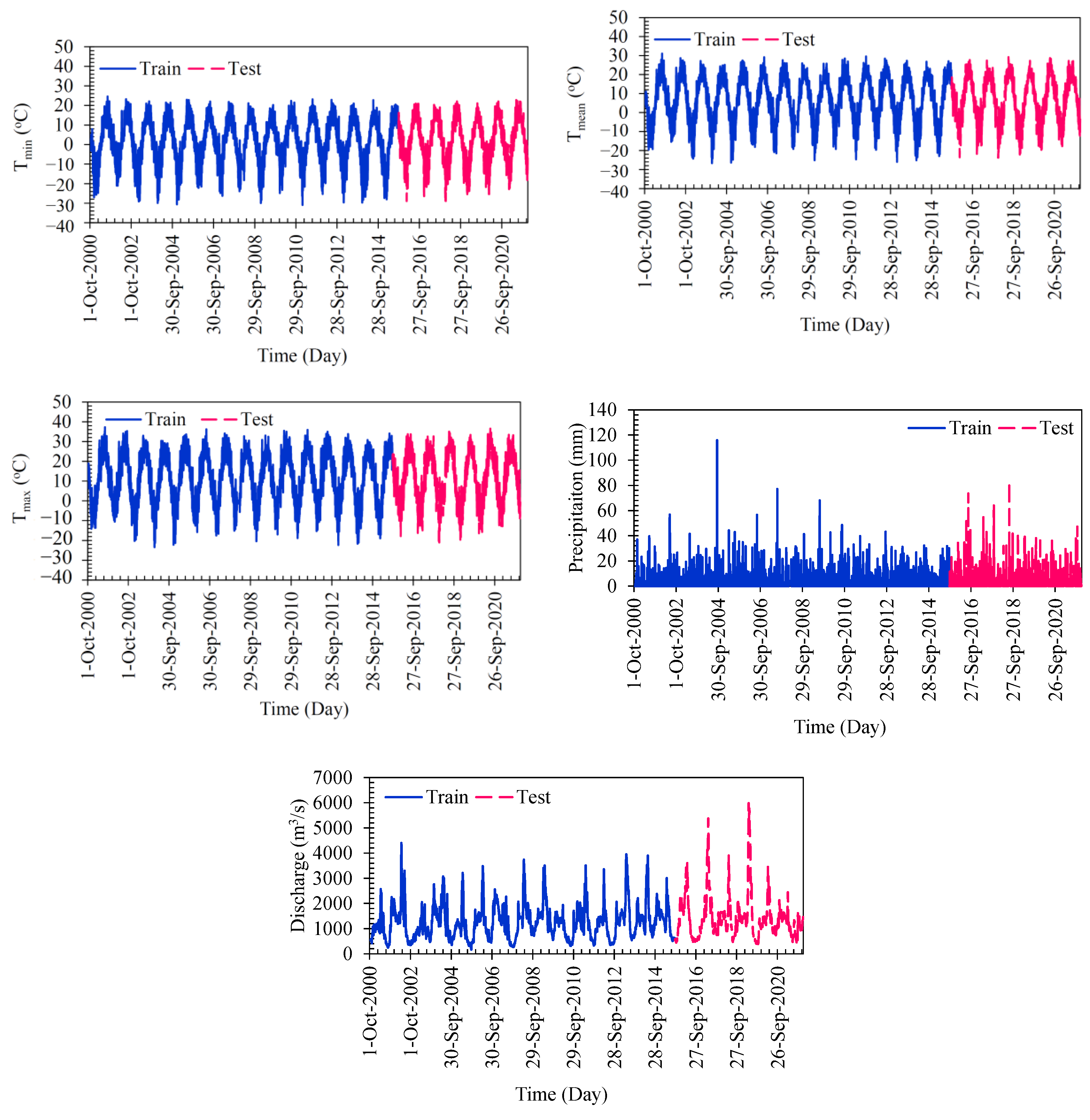
The main objective of this study is to develop a practical model for daily river flow modeling by fusing machine learning algorithms. In this study, the input variables used for daily river flow discharge forecasting include minimum, mean, and maximum temperature, precipitation, and discharge with a single lead time. The dataset utilized for model training and evaluation was collected from 21 October 2000, to 31 December 2021, encompassing a total of 7546 samples. Once the ASGMDH model was calibrated, its performance was thoroughly assessed through qualitative and quantitative evaluations. Additionally, uncertainty and reliability analyses were conducted to further scrutinize the model’s performance and provide insights into its reliability in real-world applications. Furthermore, the sensitivity of the developed model to each of the input variables was examined using partial derivative sensitivity analysis, enabling a better understanding of the significance of each variable in the modeling process. These comprehensive assessments and analyses contribute to a thorough understanding of the ASGMDH model’s capabilities and provide valuable insights for its practical application in daily river flow forecasting, supporting water resource management, and decision-making processes.

2. Materials and Methods

2.1. Study Area

The study area focuses on the Ottawa River, a prominent water body in Eastern Canada (Figure 1). The river flows through two Canadian provinces, Ontario and Quebec, serving as a natural boundary between them. With a length of 1271 km, it ranks as the second-longest river in Eastern Canada. The Ottawa River originates from Lake des Outaouais, situated in Quebec, approximately 250 km north of Ottawa, the capital city of Canada. The lake, located at an elevation of 430 m, serves as the source of the river. From there, the Ottawa River meanders through diverse landscapes, including forests, urban areas, and agricultural regions, before reaching its mouth at an elevation of 20 m. Notably, the Ottawa River holds significant hydrological importance as the primary tributary to the St. Lawrence River, one of the major waterways in North America. The river’s expansive watershed covers an area of approximately 146,300 km2. This extensive watershed encompasses various ecosystems and landforms, contributing to the complexity of the river’s hydrological processes. The Ottawa River exhibits significant variations in flow rates. The maximum observed discharge within our study period occurred on 1 May 2019, reaching a value of 5980 m3/s. Conversely, the minimum discharge occurred on 25 September 2005, with a value of 165 m3/s. These extreme values highlight the dynamic nature of the river and the wide range of flow conditions it experiences. Such variations in discharge emphasize the need for accurate prediction models to effectively manage and mitigate flood risks in the region.
Figure 2 visually represents the distribution of the five variables used in developing the machine learning model. These variables include river discharge (m3/s), minimum and maximum air temperatures (°C), mean temperature (°C), and precipitation (mm). The figure showcases how these variables vary over time in the study area, encompassing both the training and testing stages of the model. By examining the distribution of these variables, valuable insights can be gained regarding the dynamics and patterns of the study area’s hydrological and climatic conditions. The river discharge variable illustrates the fluctuation in water flow rates, highlighting high and low discharge periods. The air temperature variables, including the minimum, maximum, and mean temperatures, provide a comprehensive understanding of the area’s temperature range throughout the observed period. Additionally, the precipitation variable indicates the amount and variability of rainfall over time. The study area experienced a significant flood event in May 2019, which stands out as the most important flood in the recorded data. This flood was characterized by a river discharge of 5980 (m3/s) on the first of May. Analysis of the results revealed that the primary contributing factors to this flood were the high precipitation levels observed in April 2019, combined with a heatwave that occurred towards the end of May. The heatwave led to snow melting, exacerbating the flood event in the study area. Notably, all peak river flows in the area were observed during spring, indicating that spring floods are the most common occurrence in this region. This finding held significant importance for the development of the machine learning model. Unlike the conventional approach that primarily considers previous lags in daily river flow prediction, we incorporated temperature as an additional input parameter. This inclusion aimed to account for the impact of the heatwave-induced snow melting, a crucial natural event affecting flood prediction in the study area. By incorporating temperature into the predictive model, we aimed to capture the intricate relationship between temperature variations, snow melt, and subsequent river flow. This approach recognizes the unique hydrological dynamics of the study area and enables more accurate and reliable flood predictions. The integration of temperature as an input parameter aligns with the need to account for the specific factors influencing regional flood occurrences, providing a more comprehensive and robust prediction model. The data used for model development spanned from October 2000 until December 2021. The dataset was divided into two subsets: 70% of the data, covering the period from October 2000 to September 2015, was used for training, while the remaining 30% was allocated for testing purposes.
Table 1 summarizes the descriptive statistics of the variables at the training and testing stages. The maximum and minimum values in Table 1 reveal important insights about the range and extremities of the variables. Analyzing the discharge variable, we find that the maximum discharge recorded during the study period is 4400 (m3/s) in the training set and 5980 (m3/s) in the testing set. Conversely, the minimum discharge is 165 (m3/s) in the training set and 330 (m3/s) in the testing set. These extreme values indicate the potential for significant variations in water discharge, with the testing data exhibiting a wider range of values compared to the training data. Analyzing the discharge variable, we observe that the mean discharge values in the training and testing sets are 1261.72 (m3/s) and 1417.57 (m3/s), respectively. The median values provide a measure of the central tendency, with 1190 (m3/s) in the training set and 1260 (m3/s) in the testing set. The standard deviation is 690.84 (m3/s) for the training set and 886.25 (m3/s) for the testing set, indicating greater variability in discharge values in the testing data. Turning to the precipitation variable, we observe a maximum precipitation value of 115.8 (mm) in the training set and 83 (mm) in the testing set. Conversely, the minimum precipitation values are zero in the training and testing sets, indicating periods of no recorded precipitation in the study area. Examining the precipitation variable, we find that the mean values are 2.35 (mm) in the training set and 2.60 (mm) in the testing set. The standard deviation is 5.74 (mm) in the training set and 6.52 (mm) in the testing set, suggesting slightly higher variability in precipitation measurements in the testing data. Regarding the temperature variables (Tmax, Tmin, and Tmean), the maximum and minimum values provide insights into the temperature extremes experienced. The maximum values indicate the highest recorded temperatures, with 37.1 °C for Tmax, 36.4 °C for Tmin, and 30.9 °C for Tmean in the training set. Similarly, the testing set shows maximum values of 36.4 °C for Tmax, 36.4 °C for Tmin, and 29.1 °C for Tmean. On the other end of the spectrum, the minimum values represent the lowest recorded temperatures, with −23.2 °C for Tmax, −20.9 °C for Tmin, and −26.5 °C for Tmean in the training set, and −30.7 °C for Tmax, −28.9 °C for Tmin, and −23.7 °C for Tmean in the testing set. For the temperature variables (Tmax, Tmin, and Tmean), the mean values are relatively close in both sets, indicating consistency. The standard deviations are slightly higher in the testing set, implying greater variability in temperature measurements during the testing period. The skewness values, which are negative for all temperature variables, indicate a slight left-skewness in the distribution of temperature data.

2.2. Machine Learning Technique

The Group Method of Data Handling (GMDH) proposed by Ivakhnenko [43] is an inductive algorithm for mathematical modeling and data analysis. It is a self-organizing system that aims to construct a mathematical model based on input-output relationships in a given dataset. The GMDH algorithm is capable of solving complex nonlinear problems by automatically optimizing the structure and parameters of the model [41,44,45]. It employs a unique approach where a model is constructed as a network of interconnected neurons, where each neuron in a layer is formed by connecting different pairs of neurons from the previous layer using a quadratic polynomial. This process generates new neurons in subsequent layers, facilitating the modeling of complex relationships between inputs and outputs. This flexible representation enables GMDH to effectively map inputs to one or more outputs, making it a valuable tool for tackling intricate problems that require capturing nonlinear dynamics in various modeling and prediction tasks [46,47]. The GMDH algorithm is designed to minimize the computational error between the observed output variable yi and the predicted output y ^ i . It achieves this by constructing a model ( f ^ i ) that maps the input variables X = (x1, x2, x3, …, xn) (where n is the number of input variables) to the predicted output y ^ i . GMDH leverages its self-organizing capability to build a network of interconnected neurons, where each neuron represents a 2nd order polynomial function involving various combinations of the input variables. By optimizing the structure and parameters of this network, GMDH aims to achieve a model ( f ^ i ) that provides the closest approximation to the actual output (yi) based on the given inputs (xi1, xi2, xi3, …, xin). Thus, GMDH operates by minimizing the computational error between the observed and predicted output, resulting in an effective modeling approach, as shown in Figure 3.
By finding an optimal function, the GMDH-type neural network aims to minimize the squared difference between the actual output (yi) and the predicted output ( y ^ i ). This minimization objective can be expressed as:
O F = M i n y ^ i = 1 M ( y ^ i y i ) 2
where OF is the objective function, M is the total number of data samples, and yi and y ^ i are the ith samples of the actual and predicted output.
The relationship between input variables and the predicted output variable can be expressed using a complex discrete form of the Volterra functional series, known as the Kolmogorov-Gabor polynomial. This polynomial takes the form:
y ^ = q 0 + i = 1 M q i x i + i = 1 M j = 1 M q i j x i x j + i = 1 M j = 1 M k = 1 M q i j k x i x j x k +
where y ^ i is the predicted output value, {q0, qi, qij, qijk} ae unknown coefficients, xi, xj, and xk are ith, jth, and kth input variables (respectively), and M is the total number of data samples.
This polynomial captures the general connection between the input variables and the output variable, with each term representing the contribution of different combinations of the input variables. The coefficients (q0, qi, qij, qijk, ...) determine the impact of each term on the overall relationship. The Kolmogorov-Gabor polynomial provides a flexible and expressive representation for modeling complex nonlinear relationships between inputs and outputs, allowing for capturing intricate patterns and interactions within the data. This polynomial captures the general connection between the input variables and the output variable, with each term representing the contribution of different combinations of the input variables. The unknown coefficients (q0, qi, qij, qijk, ...) determine the impact of each term on the overall relationship. In the context of the given equation and description, the input vector X = (x1, x2, ..., xn) represents a collection of input variables. The unknown coefficients qᵢ (i = 1, 2, 3, 4, 5) in the equation correspond to the weights vectors or polynomial coefficients associated with each term in the polynomial series. These coefficients determine the influence and contribution of each input variable xi in the overall relationship between the inputs and the output variable. By adjusting the values of these coefficients, the model can capture the complex interactions and patterns between the inputs and outputs, enabling effective modeling and prediction of the relationship between the variables. The complete mathematical description can be simplified as a partial quadratic polynomials system consisting of two variables (neurons). The simplified form takes the following structure:
y ^ = G ( x i , x j ) = q 1 + q 2 x i + q 3 x j + q 4 x i 2 + q 5 x j 2 + q 6 x i x j
where xi and yi represent the input variables, while q0, q1, q2, q3, q4, and q5 are the unknown coefficients or weights associated with the polynomial terms. Each term in this equation represents the contribution of different combinations of the input variables and their quadratic forms. By adjusting the values of the coefficients, the model can effectively capture and represent the complex interactions and patterns between the input variables, resulting in improved modeling and prediction capabilities. In the basic form of the GMDH algorithm, all possible combinations of two independent variables from a total of n input variables (xi, i = 1, 2, 3, ..., M) are considered to construct a regression polynomial in the form of quadratic polynomials with only two variables that best fit the dependent observations (yi, i = 1, 2, ..., M) in a least-squares sense. The number of neurons in the first hidden layer is determined by the number of these combinations, which is given by (n,2) = n(n1)/2, (where n is the number of input variables). Therefore, n(n1)/2 neurons are built in the first hidden layer based on the observed data. Each neuron in the hidden layer represents a specific combination of two input variables. By systematically exploring all these combinations, the GMDH algorithm aims to construct a practical model that captures the underlying relationships and patterns in the data. The least-squares approach is used to optimize the fit between the model’s predictions and the actual observations, ensuring a robust and accurate data representation. Each neuron represents a combination of variables (xia, xin) from the input vector {(yi, xia, xib); (i = 1, 2, 3, ..., M) (a, b∈{1, 2, 3, ..., n})}. The model is defined as follows:
{ y 1 = q 0 + q 1 x 1 a + q 2 x 1 b + q 3 x 1 a x 1 b + q 4 x 1 a 2 + q 5 x 1 b 2 y 2 = q 0 + q 1 x 2 a + q 2 x 2 b + q 3 x 2 a x 2 b + q 4 x 2 a 2 + q 5 x 2 b 2 y M = q 0 + q 1 x M a + q 2 x M b + q 3 x M a x M b + q 4 x M a 2 + q 5 x M b 2
where yi represents the observed output variable for the ith observation, and Q = {q0, q1, q2, q3, q4, q5} is the vector of polynomial coefficients. The y values can be represented by the equation y = Aa. The matrix A represents the input variables:
A = [ 1 x 1 a x 1 b x 1 a x 1 b x 1 a 2 x 1 b 2 1 x 2 a x 2 b x 2 a x 2 b x 2 a 2 x 2 b 2 . . . . . . . . . . . . . . 1 x M a x M b x M a x M b x M a 2 x M b 2 ]
and y is the vector of observed output variables y = [y1, y2, y3, ..., yM]. The goal is to find the optimal coefficients Q = {q0, q1, q2, q3, q4, q5} that minimize the difference between predicted and observed output values.
The classical GMDH encounters several limitations in daily river flow predictions, including (i) Restriction to 2nd-order polynomial structure, (ii) Limitation in the number of variables that can serve as inputs to neurons (only two variables allowed), (iii) Limited use of neurons solely from adjacent layers. To overcome these limitations, a new scheme is introduced to assess the impact of more complex models on improving the predictive performance of GMDH. This modified GMDH model allows for generating 2nd and 3rd-order polynomials with two and three inputs, respectively, within each polynomial. As a result, three additional polynomial forms, in addition to the previously mentioned 2nd-order polynomial in Equation (3), are defined as follows:
y ^ = G ( x i , x j , x k ) = q 0 + q 1 x i + q 2 x j + q 3 x k + q 4 x i 2 + q 5 x j 2 + q 6 x k 2 + q 7 x i x j + q 8 x 1 x k + q 9 x j x k
y ^ = G ( x i , x j ) = q 0 + q 1 x i + q 2 x j + q 3 x i 2 + q 4 x j 2 + q 5 x i x j + q 6 x i x j 2 + q 7 x i 2 x j + q 8 x i 3 + q 9 x j 3
y ^ = G ( x i , x j , x k ) = q 0 + q 1 x 1 + q 2 x 2 + q 3 x 3 + q 4 x 1 2 + q 5 x 2 2 + q 6 x 3 2 + q 7 x 1 x 2 + q 8 x 1 x 3 + q 9 x 2 x 3 + q 10 x 1 3 + q 11 x 2 3 + q 12 x 3 3 + q 13 x 1 2 x 2 + q 14 x 1 2 x 3 + q 15 x 2 2 x 1 + q 16 x 2 2 x 3 + q 17 x 3 2 x 1 + q 18 x 3 2 x 2 + q 19 x 1 x 2 x 3
Based on these equations, it is evident that the 2nd-order polynomial with three inputs (Equation (6)) and the 3rd-order polynomial with two inputs (Equation (7)) each have ten unknown coefficients. However, the 3rd-order polynomial with three inputs (Equation (8)) has twenty unknown coefficients. This new scheme of GMDH is known as the Adaptive Structure of GMDH (ASGMDH), which can dynamically adapt and optimize itself based on the available data or changing input patterns. This adaptability enables the model to effectively capture and represent complex relationships and patterns in the data. By incorporating an adaptive structure into the GMDH method, the model can enhance its capacity to handle diverse datasets, optimize its performance, and improve its predictive accuracy. In the ASGMDH, an additional improvement is the automatic selection of input variables. This means that not all inputs are necessarily included in the final version of the model, which is a combination of one or more polynomials. Essentially, this method autonomously conducts feature selection during the process of generating optimal polynomials. This feature selection capability is beneficial because it allows the model to identify and incorporate only the most relevant input variables, thereby reducing dimensionality and potentially improving its predictive performance. By automatically selecting the inputs that contribute the most to the model’s accuracy, the ASGMDH optimizes the representation of the underlying relationships within the dataset.
The objective function of the ASGMDH is established using the corrected version of the Akaike Information Criteria (AICc) [48,49]. It comprises two primary components: an accuracy term and a complexity term. The accuracy term focuses on assessing the model’s ability to predict accurately. It takes into account how well the model captures the underlying patterns and relationships present in the dataset. This term aims to maximize the accuracy or goodness-of-fit of the model to the observed data. On the other hand, the complexity term accounts for the complexity or simplicity of the model. It penalizes overly complex models, thereby aiming to avoid overfitting and promote model parsimony. The complexity term discourages the inclusion of unnecessary variables or incredibly intricate model structures that may lead to decreased generalization performance on new, unseen data. Combining these two terms within the objective function, the ASGMDH seeks to strike a balance between accuracy and model complexity. The goal is to find the optimal model that achieves a good balance between capturing the patterns in the data while keeping the model as simple and interpretable as possible.
A I C c = M × L n ( 1 M i = 1 M ( Q A t Q P t ) 2 ) + 2 K M K M 1
where M is the number of samples, Q A t and Q P t are the actual and predicted (respectively) flow discharge at tth sample, and K is the number of tuned parameters of the desired model. All the codings for implementing the classical GMDH and ASGMDH have been done in MATLAB.

2.3. Statistical Measures

This paper used four statistical indices to evaluate and assess the performance of the machine learning models. The coefficient of Determination (R2) represents the proportion of the variance in the dependent variable (predicted values) that can be explained by the independent variables (input features). It ranges from 0 to 1, with a higher value indicating a better fit between the predicted and actual values. R2 is commonly used to measure the goodness of fit and overall performance of a model. A high R2 value suggests that the model captures a significant portion of the variability in the data. Normalized Root Mean Squared Error (NRMSE) measures the average magnitude of the residuals (differences between predicted and actual values) relative to the range of the dependent variable. It is calculated as the ratio of the root mean squared error to the range of the dependent variable. NRMSE provides a normalized measure of the model’s error, allowing for better comparison across different datasets. A lower NRMSE indicates a more accurate model, representing a smaller average deviation from the actual values. Mean Absolute Relative Error (MARE) measures the average relative difference between the predicted and actual values. It is calculated as the mean of the absolute differences divided by the mean of the actual values. MARE provides a measure of the average percentage error of the model. It is advantageous when the magnitude of the error relative to the actual values is important. A lower MARE indicates a more accurate model, representing a smaller average percentage deviation from the actual values.
R 2 = ( t = 1 M ( Q A t Q ¯ A ) ( Q P t Q ¯ P ) t = 1 M ( Q A t Q ¯ A ) 2 t = 1 M ( Q P t Q ¯ P ) 2 ) 2
N R M S E = 1 M t = 1 M ( Q A t Q P t ) 2 1 M t = 1 M Q A t
M A R E = 1 M t = 1 M | Q A t Q P t Q A t |
N S E = 1 t = 1 M ( Q A t Q P t ) 2 t = 1 M ( Q A t Q ¯ A ) 2
where M is the number of samples, Q A t and Q P t are the actual and predicted (respectively) flow discharge at tth sample, Q ¯ A and Q ¯ P are the average of the actual and predicted flow discharge, respectively. These four indices collectively comprehensively evaluate the model’s performance [50,51]. While R2 assesses the overall goodness of fit, NRMSE, MARE, and NSE, provide measures of the model’s accuracy, precision, and relative performance compared to a benchmark. By considering multiple indices, researchers can gain a more robust understanding of the model’s strengths and weaknesses, leading to improved model selection, refinement, and better overall accuracy.

2.4. Reliability Analysis

To gauge the reliability of measurements and determine whether the observed results are consistent and reproducible, the Reliability analysis (RA) can be performed. RA is a statistical method used to assess the consistency, stability, and dependability of measurements, scales, or tests. More precisely, it assesses whether a proposed model reaches an acceptable level of performance. The primary goal of RA is to determine the extent to which the measurements obtained from a particular approach are dependable and free from random error. It helps researchers or practitioners assess whether the approach consistently estimates what it intends to evaluate over time, across different conditions, or among different individuals. RA provides practitioners with valuable insights into the quality and consistency of applied tools, allowing them to make informed decisions regarding using specific approaches in their practice. It helps ensure the techniques employed are reliable, valid, and suitable for the intended analysis or interpretation. The RA is defined as follows:
R A = 100 M t = 1 M R t
where
R t = { 0 | Q A t Q P t Q A t | > α 1 | Q A t Q P t Q A t | α
where Q A t and Q P t are the actual and predicted (respectively) flow discharge at the tth sample, and α is the acceptable relative error. The value of α is project-dependent and can vary based on specific requirements. However, as a general guideline, it is often suggested that the maximum value of α should be set to 0.2 or 20% [40,52]. The current study examines various values for α, including 0.01, 0.02, 0.05, 0.1, 0.15, and 0.2.

2.5. Uncertainty Analysis

Uncertainty analysis is utilized to examine the expected range of a model or experiment, precisely the uncertainty interval (UI) that approximates the discrepancy between estimated and actual values. U95, a well-known technique for calculating the UI, is interpreted as follows: “Through repeated experimentation, the true value of the test result is expected to fall within the UI approximately 95 times out of 100 experiments” [52]. The definition of U95 is as follows:
U 95 = 1.96 M t = 1 M ( Q A t Q ¯ A ) 2 + t = 1 M ( Q A t Q P t ) 2
where Q A t and Q P t are the actual and predicted (respectively) flow discharge at the tth sample, and M is the total number of data samples.

3. Results and Discussions

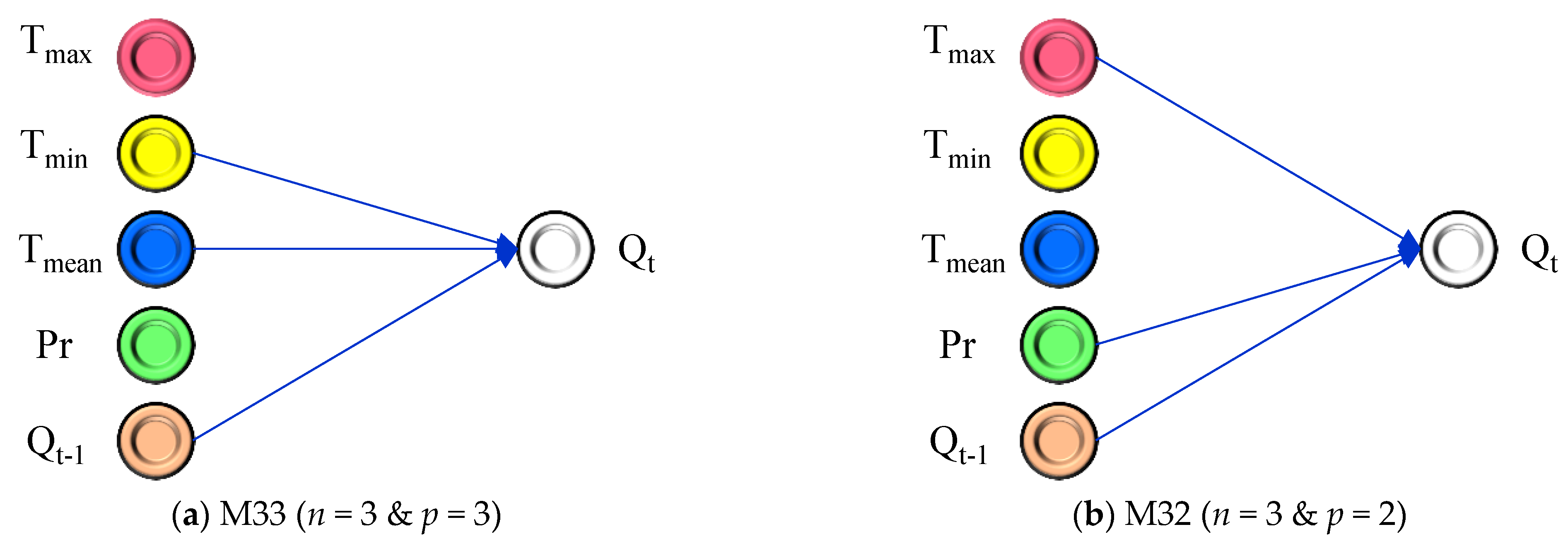
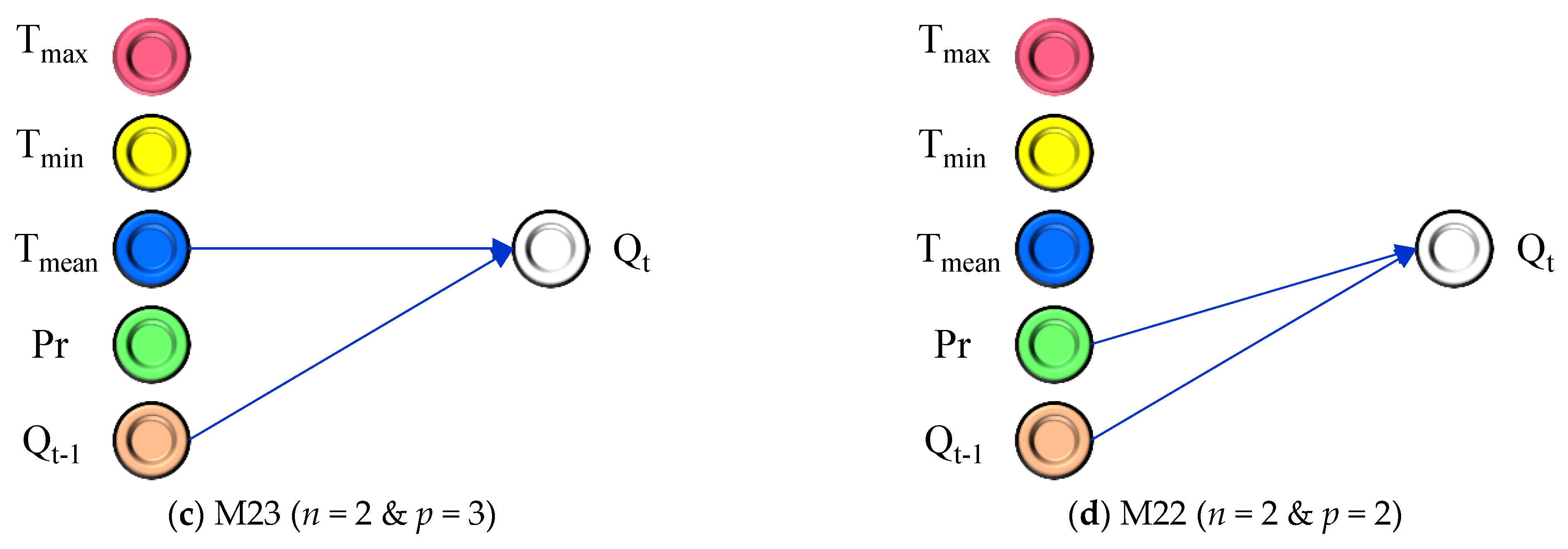
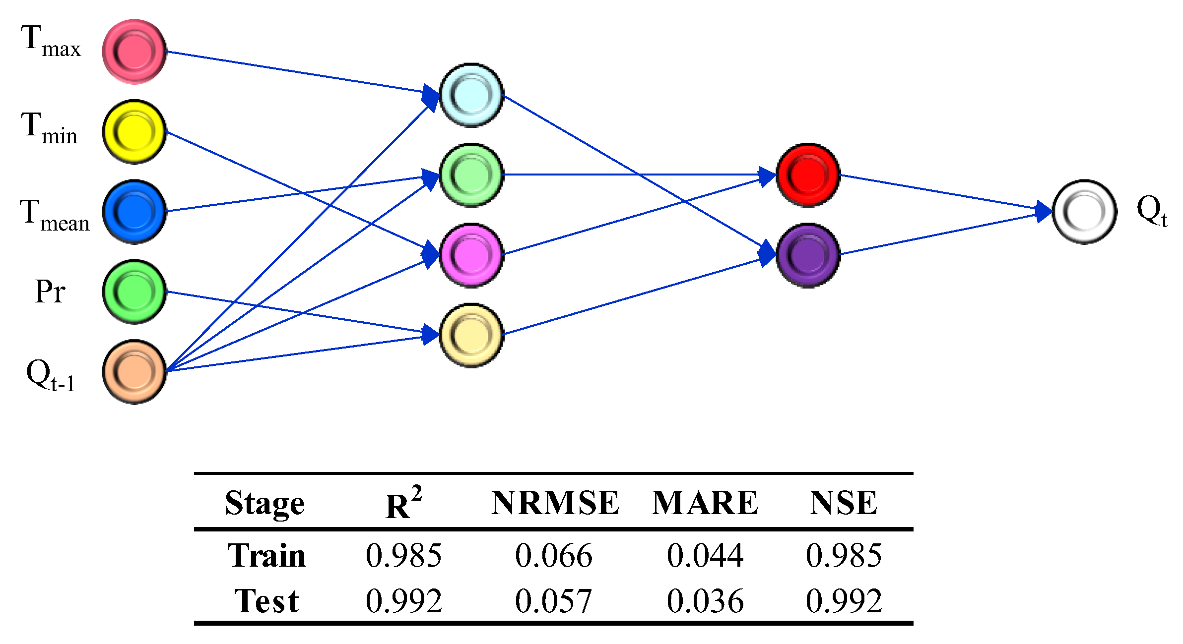
The river flow prediction in this study involved the consideration of five different inputs. These inputs included the measured discharge from the previous day, which served as a historical record summarizing watershed characteristics. Additionally, real-time data on air temperatures (minimum, maximum, and mean) and precipitation were incorporated. The development of the Adaptive algorithm, known as ASGMDH, introduced significant improvements to the traditional GMDH approach. ASGMDH allowed for the inclusion of second and third-order polynomials, with two or three different inputs in each polynomial. This enhancement resulted in four distinct scenarios, as illustrated in Figure 4. These scenarios not only improved the main structure of the polynomial used in the classical GMDH but also incorporated a feature selection technique. This feature selection technique enhanced the model’s performance and flexibility.
Figure 4 demonstrates the different combinations of variables used in each scenario. In the case of model M33, Tmin, Tmean, and Qt−1 were utilized to predict the output, employing a polynomial equation with a degree of three. In M32, Tmax, Pr, and Qt−1 were used with a polynomial equation of degree two. For model M23, Tmean and Qt−1 were combined in a polynomial equation of degree three. Lastly, in model M22, Pr and Qt−1 were employed with a polynomial equation of degree two. By incorporating these different scenarios, the ASGMDH model demonstrated improved adaptability and accuracy in predicting river flow. The selection of specific variables and the utilization of polynomial equations with varying degrees contributed to the model’s effectiveness in capturing the complex relationships within the data. As highlighted in Figure 4, it is evident that all the models have a single layer in their final structure. However, there are three key differences in the structure of these developed models: (i) the number of inputs in the generated polynomial, (ii) the polynomial degree for each one, and (iii) the type of input variables. Referring to Figure 4, the models with three inputs are M33 (Equation (13)) and M32 (Equation (14)), while the models with two input variables are M23 (Equation (15)) and M22 (Equation (16)). Additionally, the models M32 (Equation (14)) and M22 (Equation (16)) employ 2nd-order polynomials, whereas the models M33 (Equation (13)) and M23 (Equation (15)) utilize 3rd-order polynomials.
In the case of input variables for river flow discharge forecasting, it is observed that the selected inputs from the five provided options are below the maximum limit. Across all the developed models, which vary in polynomial types and the allowed number of inputs in each polynomial, different inputs have been identified as the most influential variables for daily river flow forecasting.
Q t = 51.95 + 1.07 × Q t 1 + 29.33 × T m e a n 28.30 × T min 16.07 E 3 × T m e a n × Q t 1   + 17.59 E 3 × T min × Q t 1 + 8.58 × T min × T m e a n 1.84 E 05 × Q t 1 2 4.54 × T m e a n 2   3 . 88 × T min 2 2.14 E 3 × T min × T m e a n × Q t 1 + 1.46 E 06 × T m e a n × Q t 1 2   + 9.67 E 4 × T m e a n 2 × Q t 1 1.42 E 06 × T min × Q t 1 2 0.53 × T min × T m e a n 2   + 1.03 E 3 × T min 2 × Q t 1 + 0.47 × T min 2 × T m e a n + 1.4 E 09 × Q t 1 3 + 0.194 × T m e a n 3 0.14 × T min 3
Q t = 25.07 + 0.98 × Q t 1 + 0.235 × P + 0.644 × T max   + 3.49 E 4 × P × Q t 1 1.79 E 4 × T max × Q t 1 + 21.97 E 3 × T max × P   + 2.29 E 06 × Q t 1 2 + 51.4 E 4 × P 2 54.05 E 3 × T max 2
Q t = 0.68 + 1.02 × Q t 1 1.398 × T m e a n + 14.59 E 4 × T m e a n × Q t 1   1.39 E 05 × Q t 1 2 + 0.144 × T m e a n 2 + 1.425 E 07 × T m e a n × Q t 1 2 14.47 E 5 × T m e a n 2 × Q t 1 + 1.64 E 09 × Q t 1 3 29 . 06 E 4 × T m e a n 3  
Q t = 3.157 + 0.998 × Q t 1 + 0.804 × P + 28.66 E 5 × P × Q t 1 1.87 E 6 × Q t 1 2 + 34.55 E 4 × P 2
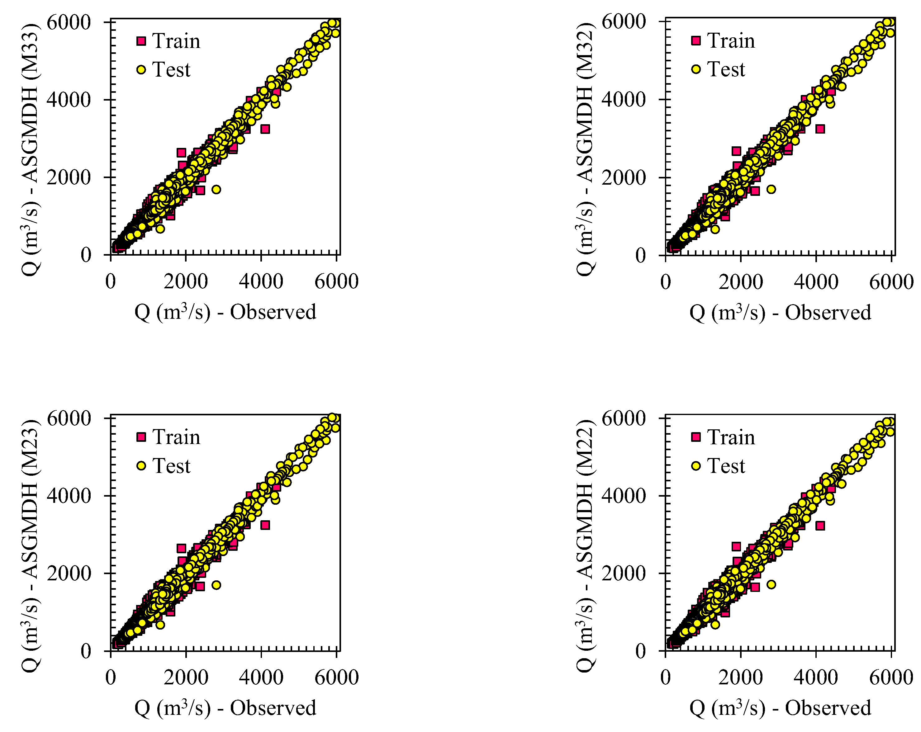
Scatter plots depicting the daily river flow discharge for four ASGMDH-based models during both the training and testing stages are presented in Figure 5. The grand line in the scatter plot represents a perfect match between the observed daily discharge values (Q) and the predicted values from all four equations in the train and test stages. A diagonal line signifies a strong positive linear relationship between observed and predicted values. Closer proximity to the grand line indicates a higher degree of agreement and a better fit of the equation to the observed data. The predicted values in all four scenarios follow almost the same prediction pattern compared to the observed values. The similarity in prediction patterns suggests that all four equations are capable of capturing the underlying patterns and trends in the observed daily discharge. This consistency in predictions further supports the reliability and effectiveness of the equations in estimating the daily discharge values.
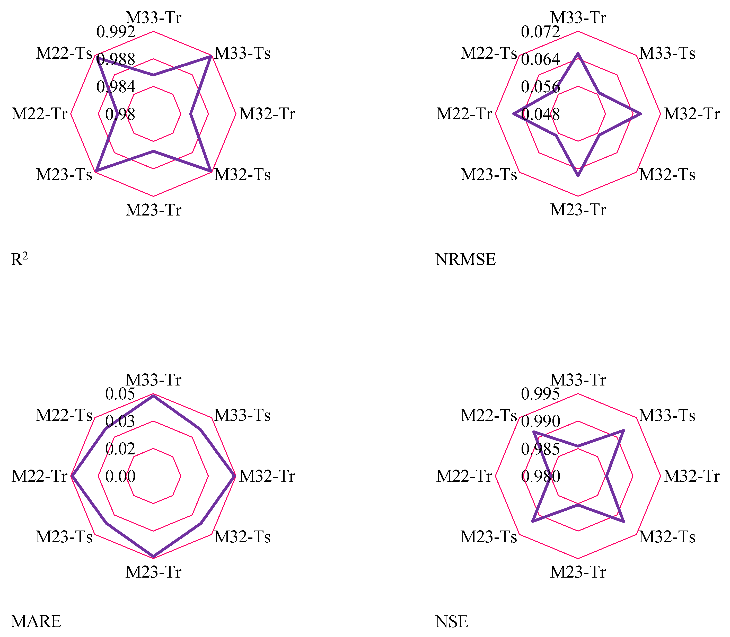
Figure 6 displays the statistical indices for the ASGMDH-based models developed for daily river flow forecasting. The R2 values for all models and datasets range from 0.985 to 0.992, indicating a strong correlation between the predicted and observed river flow values. The models explain a significant portion of the variance in the data, suggesting their effectiveness in capturing the underlying patterns. The NRMSE values for all models and datasets are relatively low, ranging from 0.057 to 0.067. This indicates that the models have a good level of accuracy in predicting river flow values, with small deviations from the observed data. The MARE values for all models and datasets range from 0.036 to 0.044, indicating a low average relative error in the predictions. The models perform well in estimating the river flow values with good precision. The NSE values for all models and datasets are high, ranging from 0.985 to 0.992. This indicates a strong agreement between the predicted and observed values, highlighting the models’ ability to accurately reproduce the observed river flow patterns. Overall, the statistical indices demonstrate the strong performance and accuracy of the developed models. The high R2, low NRMSE, MARE, and high NSE values indicate that the models can effectively capture the relationships between the input variables and river flow, providing reliable predictions. These results validate the effectiveness of the proposed ASGMDH approach for daily river flow modeling and emphasize its potential for practical applications in water resource management and decision-making processes.
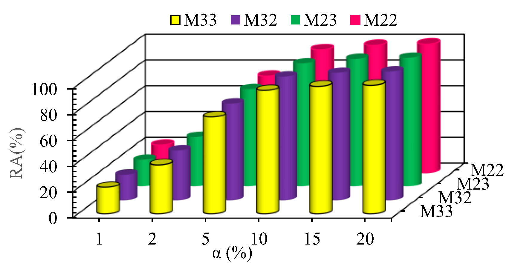
Figure 7 illustrates the reliability analysis results conducted for the ASGMDH-based models, considering different values of α as provided in Equation (15). The figure reveals a clear correlation between the α value and the reliability analysis (RA) value. Specifically, the models exhibit the highest (or lowest) RA values corresponding to the highest (or lowest) α values. Notably, the α values experience a relatively modest increase of less than 10%. For α values greater than or equal to 10, all models demonstrate an RA value exceeding 95%. These findings indicate the satisfactory performance of the presented ASGMDH models in accurately predicting daily river flow discharge. The RA values in Figure 7 offer more detailed insights into the model’s predictive performance. Approximately 20% of all predicted samples during the test mode exhibited a relative error of less than 1%, while 38% demonstrated a relative error of less than 2%. Furthermore, a significant proportion of samples, approximately 75%, exhibited a relative error of less than 5%. These results showcase the models’ ability to provide accurate predictions within a narrow margin of error. Additionally, the reliability analysis shows that more than 95% of all predicted samples during the test mode had a relative error of less than 10%. Moreover, approximately 98% of the samples demonstrated a relative error of less than 15%, while 99% exhibited a relative error of less than 20%. These findings indicate the high reliability and effectiveness of the developed ASGMDH models in accurately forecasting daily river flow discharge. The robust performance of the models, as evidenced by the high percentage of samples falling within the desired relative error thresholds, confirms their reliability in real-world flood prediction scenarios. These results provide valuable information to decision-makers in water resource management and related fields, as they can rely on the ASGMDH-based models to make informed decisions and implement effective flood mitigation and response strategies.
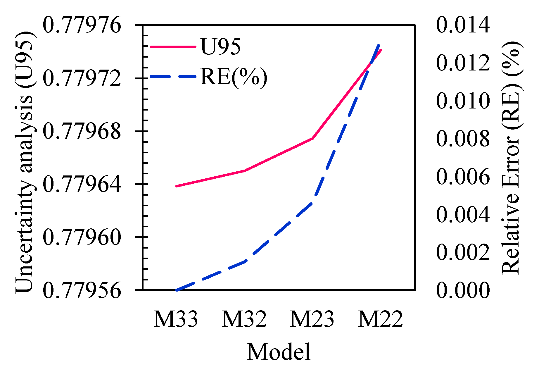
The U95 value is a measure of uncertainty and represents the upper 95% prediction interval around the predicted values. In the context of the ASGMDH-based models for daily river flow discharge, a lower U95 value indicates a narrower prediction interval. It suggests a higher level of confidence in the model’s predictions. Figure 8 presents the outcomes of the uncertainty analysis conducted on the ASGMDH-based models. The results showcase notable differences in the U95 values among the different models. Particularly, model M33, which is the most complex with 20 terms, exhibits the lowest U95 value, indicating higher confidence in its predictions. On the other hand, the simplest model, M22, consisting of only six terms, displays the highest U95 value, indicating a larger uncertainty in its predictions. A noteworthy comparison arises between two models of similar complexity, namely M33 and M32, consisting of ten terms. Surprisingly, M32, which employs a second-order polynomial with three inputs, demonstrates a lower U95 value compared to M23, which employs a third-order polynomial with two inputs. This unexpected result suggests that the predictive performance of M32 is superior, despite its lower model complexity. Furthermore, when comparing the U95 values of different models with the benchmark model M33, it is observed that the relative error values for all three cases are negligible, measuring less than 1%. These findings emphasize the high accuracy and reliability of the ASGMDH models in predicting daily river flow discharge, even for the models with lower complexity. Consequently, these results instill confidence in the effectiveness of the developed models and their capability to deliver accurate predictions with minimal uncertainty.
After evaluating the different developed models using the ASGMDH method, a model based on classical GMDH is introduced to facilitate a comparison with existing methods. Figure 9 represents the final structure of the classical GMDH model and its accuracy, where all input variables (Tmax, Tmin, Tmean, Pr, Qt−1) are included. The high R2 values indicate a strong correlation between the observed and predicted values in the training and testing stages. The low values of NRMSE and MARE suggest that the model has a small overall error, with the predicted values being close to the observed values. The NSE value of 0.985 in the training stage and 0.992 in the testing stage indicate a good model fit, where values close to 1 indicate a high level of accuracy.
However, in the presented ASGMDH models (Equations (17)–(20)), only two or three inputs are included in the final model structure. This indicates that the classical method, constrained by its limitations, fails to produce a simpler model. In contrast, the ASGMDH method employs the corrected Akaike Information Criterion (AICc) for small sample sizes to determine the final model structure, taking into account both model complexity and accuracy. This inherent feature selection capability of ASGMDH, combined with AICc, results in a simpler model with improved predictive performance. Adopting the AICc index provides a robust and objective approach for model comparison. By considering both simplicity and accuracy, it ensures that the selected model not only captures the underlying relationships in the data but also avoids overfitting and unnecessary complexity.
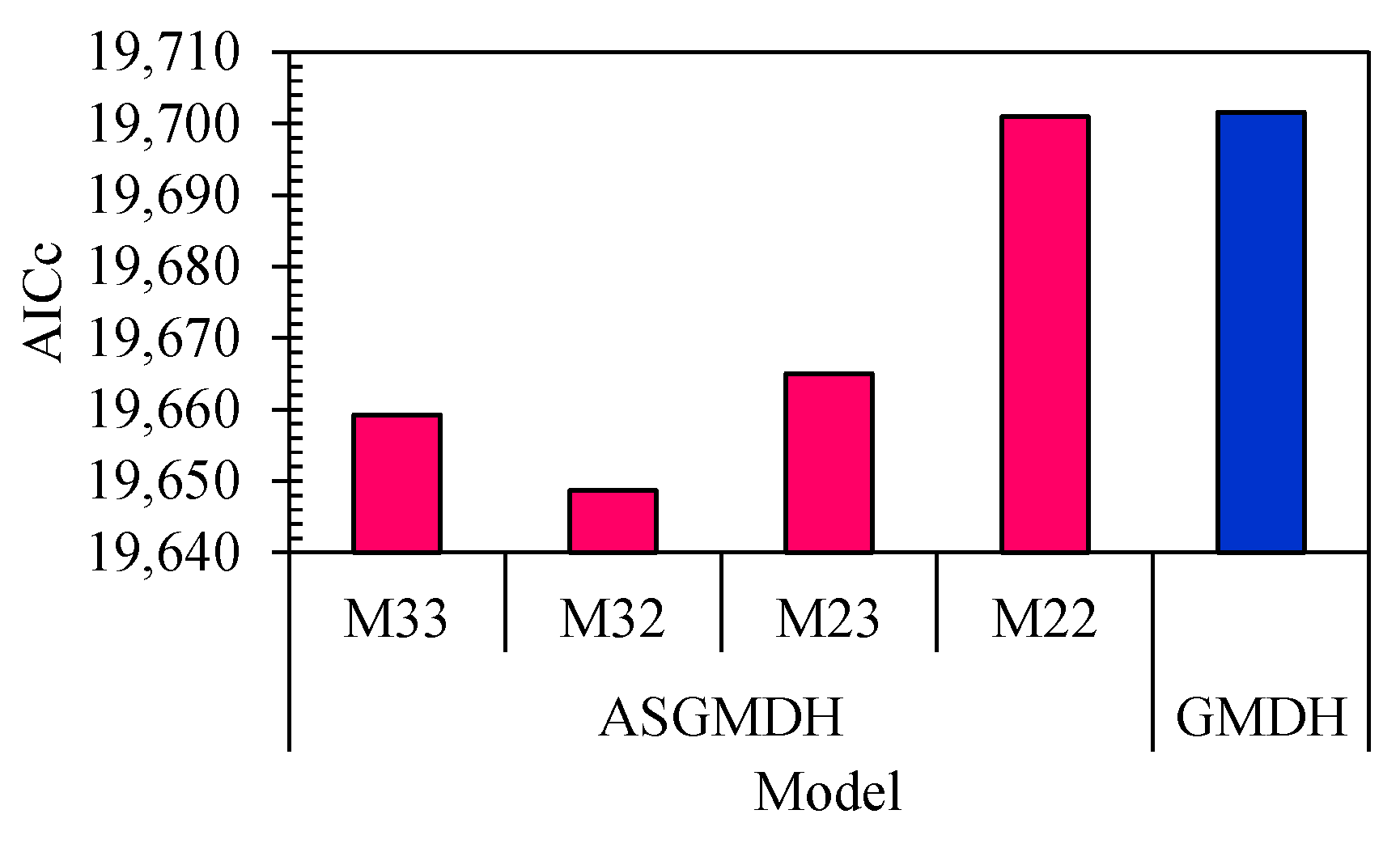
To ensure a fair comparison between the classical GMDH and ASGMDH models, the AICc index, which accounts for both simplicity and accuracy, is employed. The results depicted in Figure 10 clearly indicate that the majority of ASGMDH models have smaller AICc values compared to the GMDH model. This implies that the ASGMDH models achieve a better balance between model complexity and accuracy. Among the presented ASGMDH models, the lowest AICc value is attributed to M32, with a value of 19,648.71. Consequently, based on the AICc criterion, M32 is identified as the superior model in this study. The superiority of M32 based on the AICc criterion highlights the effectiveness of the ASGMDH method in producing a simpler yet accurate model for predicting daily river flow discharge. It is important to highlight that both models demonstrate exceptional speed in forecasting daily flow discharge. The execution time for each model is impressively quick, taking less than 2 s to complete.
To examine the changing pattern of daily river flow discharge in relation to the input variables in the ASGMDH-based model (M32), the analysis of sensitivity using the partial derivatives (PDSA) technique is utilized [53,54,55]. This approach entails assessing the sensitivity of the outcomes by measuring the partial difference between the output variable (Qt) and each individual input variable (Tmax, Pr, Qt−1). Notably, a larger partial derivative value indicates a more significant impact of the input variables on the results. When the partial derivative is positive, an increase in the input variables corresponds to a rise in the output variable, and vice versa. This approach of utilizing the PDSA technique provides valuable insights into the changing patterns of daily river flow discharge concerning the input variables. By quantifying the sensitivity of the model outputs, it enables a deeper understanding of the influence of each input variable, namely maximum temperature (Tmax), precipitation (Pr), and previous discharge (Qt−1), on the resultant river flow discharge (Qt). The magnitude and direction of the partial derivatives help identify the relative importance and directionality of the impacts.
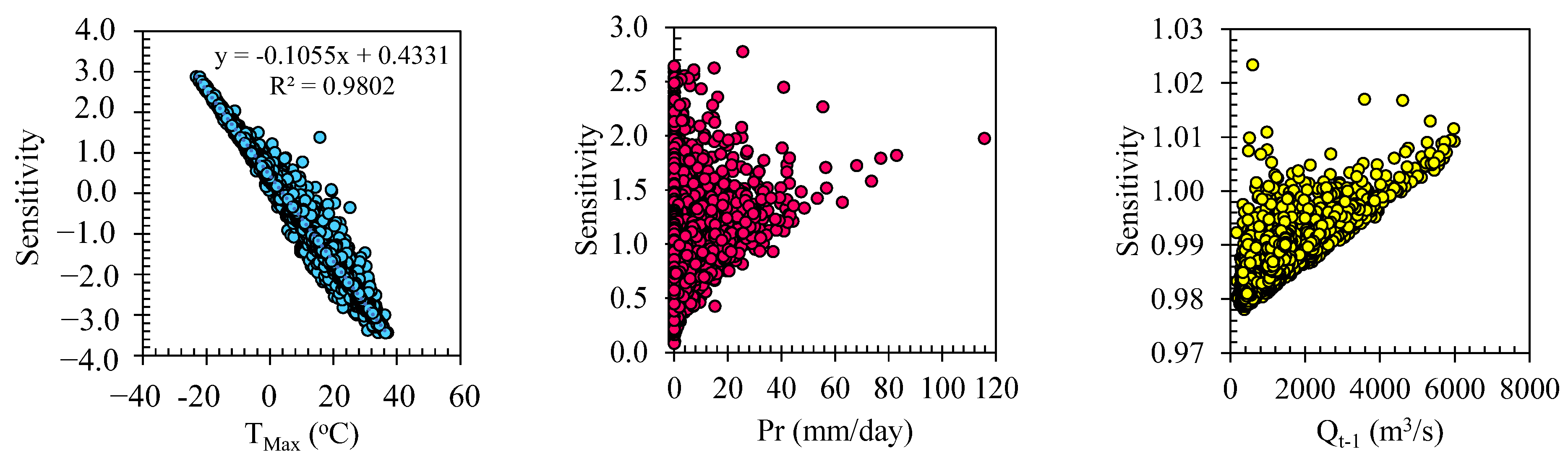
This sensitivity analysis sheds light on the intricate dynamics between the maximum temperature and river flow discharge in the ASGMDH-based model (M32). The observed linear relationship, with a negative slope, emphasizes the role of the maximum temperature as a critical driving factor for changes in daily flow discharge. Understanding this relationship enables researchers and practitioners to anticipate the effects of temperature variations on river systems and their potential impact on water resources management and flood risk assessment. These findings provide valuable insights into the model’s sensitivity and contribute to a more comprehensive understanding of the complex interplay between temperature and river flow dynamics. Figure 11 illustrates the sensitivity analysis of the ASGMDH-based model (M32) concerning the input variables utilized in the model. The graph displays the partial derivatives that reflect the sensitivity of the relationship investigated in this study, particularly concerning the maximum temperature. Overall, it can be observed that positive values of the maximum temperature correspond to negative sensitivity values, whereas negative values of the maximum temperature yield positive sensitivity values. This indicates a linear relationship with a slope of −0.1 between the maximum temperature threshold and sensitivity. As a result, when dealing with negative maximum temperature values, increasing the variable value lead to an increase in the flow discharge. Conversely, within the range of positive values, an increase in the maximum temperature result in a decrease in the daily flow discharge value calculated by the model. Indeed, suppose the model assigns greater importance to the maximum temperature value than the actual recorded value. In that case, it can lead to lower calculated flow discharge c than the expected values. This discrepancy occurs because the model becomes more sensitive to changes in the maximum temperature parameter, causing it to disproportionately influence the overall flow discharge prediction.
Among the variables examined, the maximum temperature demonstrates the highest sensitivity. The sensitivity values associated with the maximum temperature show a clear linear relationship, with negative values for positive maximum temperature values and positive values for negative maximum temperature values. This indicates that an increase in the maximum temperature leads to a decrease in the daily flow discharge, while a reduction in the maximum temperature corresponds to a rise in the discharge. Regarding precipitation, the sensitivity values consistently exhibit positive values across all ranges. For small precipitation values (Pr < 10 mm), the sensitivity values vary within the range of [0, 3]. As the precipitation value increases, the sensitivity becomes more constrained within the narrower range of [1, 2]. This suggests that precipitation positively impacts daily flow discharge, with larger precipitation events having a relatively more pronounced effect. Similarly, the sensitivity analysis reveals that Qt−1, the previous day’s flow discharge, also exerts a positive influence on the current day’s discharge. The sensitivity values for Qt−1 range from 0.97 to 1.03, indicating a relatively smaller sensitivity range compared to the other two variables. Nevertheless, an increase in the previous day’s discharge corresponds to a rise in the current day’s discharge, although the magnitude of this increase may vary across different domains. The sensitivity analysis on the input variables utilized in the developed ASGMDH-based model for daily river flow discharge prediction reveals that the maximum temperature exhibits the highest sensitivity among the variables. Following that, precipitation and Qt−1 rank as the second and third most influential variables, respectively.

4. Conclusions

This study highlights the significance of understanding flood prediction and management’s underlying factors and dynamics. Using the Adaptive Strcutre of Group Method of Data Handling (ASGMDH) model, with its explicit equations and optimization capabilities, valuable insights and accurate predictions were obtained. Notably, the sensitivity analysis revealed that the maximum temperature exhibited the highest sensitivity among the variables, followed by precipitation and Qt−1. This emphasizes the importance of considering temperature fluctuations and precipitation patterns when predicting and managing floods. Reliability and validity were ensured through a comprehensive reliability analysis, confirming the robustness of the proposed model. Furthermore, the uncertainty analysis of the ASGMDH models revealed notable differences in the U95 values across different models. Interestingly, the most complex model displayed the lowest U95 value, indicating its ability to provide more precise predictions. In addition, simpler models with fewer terms demonstrated superior predictive performance, suggesting that model complexity alone does not guarantee accuracy. This highlights the importance of model selection based on both complexity and accuracy considerations. Additionally, comparing ASGMDH models with the classical GMDH model using the AICc index demonstrated the superiority of the ASGMDH models. The ASGMDH models consistently outperformed the classical GMDH model, as indicated by their lower AICc values. The ASGMDH-based model shows a second-order polynomial (AICc = 19,648.71) in its final form, while the classical GMDH-based model has seven second-order polynomials (AICc = 19,701.56). This indicates that the ASGMDH models strike a better balance between accuracy and model complexity, offering a more robust and efficient approach for daily river flow discharge prediction. These models offer a reliable tool for water management practitioners and decision-makers, facilitating effective planning and decision-making in various water management applications. By gaining a deeper comprehension of the influence of temperature and the occurrence of spring floods, researchers and practitioners can enhance the effectiveness and applicability of machine learning techniques in flood prediction and management. The findings of this study highlight the importance of considering temperature fluctuations, precipitation levels, and historical discharge data in flood modeling. These insights, along with the reliable predictions provided by the ASGMDH model, empower decision-makers to make more accurate and effective decisions in flood management strategies, leading to improved mitigation and adaptation measures in the face of increasing flood risks. Given the valuable insights provided by the current study into historical discharge patterns, it is essential to consider the potential impact of climate change on the reliability and applicability of this model in the future. Therefore, as a natural extension of this research, the next step will comprehensively evaluate the developed model under various climate change scenarios. This evaluation will encompass the incorporation of climate projections and the utilization of the developed machine learning model, which has demonstrated promising capabilities in the current study. By integrating climate projections and advanced modeling techniques, we aim to assess the sensitivity of the model to changing climatic conditions and its ability to accurately predict future discharge patterns. This investigation is crucial, particularly for flood-prone areas along the Ottawa River, as it will enhance our understanding of the hydrological dynamics and provide a solid foundation for developing more robust and adaptive hydrological models in the face of an uncertain climate future. Moreover, this evaluation will enable us to identify the key drivers of change in discharge patterns, including the influence of climate dynamics and the intricate interactions within hydrological processes. By employing a numerical model, we can quantitatively analyze the interplay between these factors and gain insights into the mechanisms that govern the river’s response to changing climatic conditions.
The ultimate goal of this research is to improve our understanding of the Ottawa River’s hydrological behavior and its vulnerability to climate change. Refining and validating the model through this evaluation can enhance its reliability and applicability in flood forecasting and water resource management. This knowledge will empower decision-makers and stakeholders with valuable information to mitigate risks, develop effective adaptation strategies, and safeguard communities in the face of an uncertain climate future.

Author Contributions

Conceptualization, I.E. and H.B.; methodology, I.E. and H.B.; software, I.E.; validation, I.E.; formal analysis, I.E.; investigation, C.L., J.C., A.D., I.E. and H.B.; resources, C.L., J.C. and A.D.; writing—original draft preparation, C.L., J.C., A.D., I.E. and H.B.; writing—review and editing, H.B., I.E. visualization, I.E., C.L., J.C. and A.D.; supervision, H.B.; project administration, H.B.; funding acquisition, H.B. All authors have read and agreed to the published version of the manuscript.

Funding

This research was funded by Natural Sciences and Engineering Research Council of Canada (NSERC) Discovery Grant (#RGPIN-2020-04583) and the “Fond de Recherche du Québec-Nature et Technologies”, Québec Government (#B2X-315020).

Data Availability Statement

The Ottawa River flow rate data used in this study were provided by Government of Canada, https://eau.ec.gc.ca/map/index_f.html?type=historical?? (accessed on 10 May 2023).

Acknowledgments

The authors acknowledge the support of the Natural Sciences and Engineering Research Council of Canada (NSERC) Discovery Grant assessed on 1 May 2020 (#RGPIN-2020-04583) and the “Fond de Recherche du Québec- Nature et Technologies”, Québec Government assessed on 2 June 2022 (#B2X-315020). The last author (H.B.) would like to extend sincere gratitude to the International Research and Experiential Learning (IREX) office at the University of Ottawa and the International Office of ENGEES for their invaluable support in organizing and facilitating the visit of students from ENGEES to uOttawa.

Conflicts of Interest

The authors declare no conflict of interest.

References

  1. Belvederesi, C.; Dominic, J.A.; Hassan, Q.K.; Gupta, A.; Achari, G. Predicting river flow using an AI-based sequential adaptive neuro-fuzzy inference system. Water 2020, 12, 1622. [Google Scholar] [CrossRef]
  2. Mehedi, M.A.A.; Khosravi, M.; Yazdan, M.M.S.; Shabanian, H. Exploring Temporal Dynamics of River Discharge using Univariate Long Short-Term Memory (LSTM) Recurrent Neural Network at East Branch of Delaware River. Hydrology 2022, 9, 202. [Google Scholar] [CrossRef]
  3. Samui, P.; Yesilyurt, S.N.; Dalkilic, H.Y.; Yaseen, Z.M.; Roy, S.S.; Kumar, S. Comparison of different optimized machine learning algorithms for daily river flow forecasting. Earth Sci. Inf. 2023, 16, 533–548. [Google Scholar] [CrossRef]
  4. Le, X.-H.; Ho, H.V.; Lee, G.; Jung, S. Application of long short-term memory (LSTM) neural network for flood forecasting. Water 2019, 11, 1387. [Google Scholar] [CrossRef] [Green Version]
  5. Khanal, S.; Ridder, N.; De Vries, H.; Terink, W.; Van den Hurk, B. Storm surge and extreme river discharge: A compound event analysis using ensemble impact modeling. Front. Earth Sci. 2019, 7, 224. [Google Scholar] [CrossRef] [Green Version]
  6. Tehranirad, B.; Herdman, L.; Nederhoff, K.; Erikson, L.; Cifelli, R.; Pratt, G.; Leon, M.; Barnard, P. Effect of fluvial discharges and remote non-tidal residuals on compound flood forecasting in San Francisco Bay. Water 2020, 12, 2481. [Google Scholar] [CrossRef]
  7. Couasnon, A.; Eilander, D.; Muis, S.; Veldkamp, T.I.; Haigh, I.D.; Wahl, T.; Winsemius, H.C.; Ward, P.J. Measuring compound flood potential from river discharge and storm surge extremes at the global scale. Nat. Hazards Earth Syst. Sci. 2020, 20, 489–504. [Google Scholar] [CrossRef] [Green Version]
  8. Khatibi, R.; Sivakumar, B.; Ghorbani, M.A.; Kisi, O.; Koçak, K.; Zadeh, D.F. Investigating chaos in river stage and discharge time series. J. Hydrol. 2012, 414, 108–117. [Google Scholar] [CrossRef]
  9. Ismail, H.; Kamal, M.R.; Abdullah, A.F.B.; Jada, D.T.; Sai Hin, L. Modeling Future Streamflow for Adaptive Water Allocation under Climate Change for the Tanjung Karang Rice Irrigation Scheme Malaysia. Appl. Sci. 2020, 10, 4885. [Google Scholar] [CrossRef]
  10. Bonakdari, H.; Binns, A.D.; Gharabaghi, B. A comparative study of linear stochastic with nonlinear daily river discharge forecast models. Water Resour. Manag. 2020, 34, 3689–3708. [Google Scholar] [CrossRef]
  11. Rath, A.; Swain, P.C. Evaluation of performance of irrigation canals using benchmarking techniques–a case study of Hirakud dam canal system, Odisha, India. ISH J. Hydraul. Eng. 2020, 26, 51–58. [Google Scholar] [CrossRef]
  12. Williams, M.R.; King, K.W. Changing rainfall patterns over the Western Lake Erie Basin (1975–2017): Effects on tributary discharge and phosphorus load. Water Resour. Res. 2020, 56, e2019WR025985. [Google Scholar] [CrossRef]
  13. Carosi, A. Effects of Climate Change on Freshwater Biodiversity. Water 2022, 14, 3953. [Google Scholar] [CrossRef]
  14. Huang, R.; Li, T.; Zhao, L. Revisiting functional no-flow events in the Lower Yellow River. Int. J. Sediment Res. 2016, 31, 351–359. [Google Scholar] [CrossRef]
  15. Dwarakish, G.; Ganasri, B. Impact of land use change on hydrological systems: A review of current modeling approaches. Cogent Geosci. 2015, 1, 1115691. [Google Scholar] [CrossRef]
  16. Laks, I.; Sojka, M.; Walczak, Z.; Wróżyński, R. Possibilities of using low quality digital elevation models of floodplains in hydraulic numerical models. Water 2017, 9, 283. [Google Scholar] [CrossRef] [Green Version]
  17. Smith, G.; Wasko, C.; Miller, B. Modelling the influence of buildings on flood flow. In Proceedings of the 52th Floodplain Management Association Conference, Batemans Bay, NSW, Australia, 21–24 February 2012. [Google Scholar]
  18. Patel, D.P.; Ramirez, J.A.; Srivastava, P.K.; Bray, M.; Han, D. Assessment of flood inundation mapping of Surat city by coupled 1D/2D hydrodynamic modeling: A case application of the new HEC-RAS 5. Nat. Hazard. 2017, 89, 93–130. [Google Scholar] [CrossRef] [Green Version]
  19. Bruno, L.S.; Mattos, T.S.; Oliveira, P.T.S.; Almagro, A.; Rodrigues, D.B.B. Hydrological and Hydraulic Modeling Applied to Flash Flood Events in a Small Urban Stream. Hydrology 2022, 9, 223. [Google Scholar] [CrossRef]
  20. Erima, G.; Kabenge, I.; Gidudu, A.; Bamutaze, Y.; Egeru, A. Differentiated Spatial-Temporal Flood Vulnerability and Risk Assessment in Lowland Plains in Eastern Uganda. Hydrology 2022, 9, 201. [Google Scholar] [CrossRef]
  21. Filianoti, P.; Gurnari, L.; Zema, D.A.; Bombino, G.; Sinagra, M.; Tucciarelli, T. An evaluation matrix to compare computer hydrological models for flood predictions. Hydrology 2020, 7, 42. [Google Scholar] [CrossRef]
  22. Mentzafou, A.; Dimitriou, E. Hydrological Modeling for Flood Adaptation under Climate Change: The Case of the Ancient Messene Archaeological Site in Greece. Hydrology 2022, 9, 19. [Google Scholar] [CrossRef]
  23. Yang, X.; Liu, Q.; He, Y.; Luo, X.; Zhang, X. Comparison of daily and sub-daily SWAT models for daily streamflow simulation in the Upper Huai River Basin of China. Stoch. Environ. Res. Risk Assess. 2016, 30, 959–972. [Google Scholar] [CrossRef] [Green Version]
  24. Yang, X.; Grönlund, A.; Tanzilli, S. Predicting flood inundation and risk using geographic information system and hydrodynamic model. Geog. Inf. Sci. 2002, 8, 48–57. [Google Scholar] [CrossRef]
  25. Jakob, M.; Holm, K.; Lazarte, E.; Church, M. A flood risk assessment for the City of Chilliwack on the Fraser River, British Columbia, Canada. Int. J. River Basin Manag. 2015, 13, 263–270. [Google Scholar] [CrossRef]
  26. Gao, P.; Gao, W.; Ke, N. Assessing the impact of flood inundation dynamics on an urban environment. Nat. Hazard. 2021, 109, 1047–1072. [Google Scholar] [CrossRef]
  27. Hao, C.; Yunus, A.P.; Subramanian, S.S.; Avtar, R. Basin-wide flood depth and exposure mapping from SAR images and machine learning models. J. Environ. Manag. 2021, 297, 113367. [Google Scholar] [CrossRef]
  28. Soltani, K.; Ebtehaj, I.; Amiri, A.; Azari, A.; Gharabaghi, B.; Bonakdari, H. Mapping the spatial and temporal variability of flood susceptibility using remotely sensed normalized difference vegetation index and the forecasted changes in the future. Sci. Total Environ. 2021, 770, 145288. [Google Scholar] [CrossRef]
  29. Grégoire, G.; Fortin, J.; Ebtehaj, I.; Bonakdari, H. Forecasting Pesticide Use on Golf Courses by Integration of Deep Learning and Decision Tree Techniques. Agriculture 2023, 13, 1163. [Google Scholar] [CrossRef]
  30. Gholami, A.; Bonakdari, H.; Ebtehaj, I.; Shaghaghi, S.; Khoshbin, F. Developing an expert group method of data handling system for predicting the geometry of a stable channel with a gravel bed. Earth Surf. Process. Landf. 2017, 42, 1460–1471. [Google Scholar] [CrossRef]
  31. Ebtehaj, I.; Bonakdari, H. Bed load sediment transport estimation in a clean pipe using multilayer perceptron with different training algorithms. KSCE J. Civil Eng. 2016, 20, 581–589. [Google Scholar] [CrossRef]
  32. Ebtehaj, I.; Bonakdari, H. Discussion of “Model Development for Estimation of Sediment Removal Efficiency of Settling Basins Using Group Methods of Data Handling” by Faisal Ahmad, Mujib Ahmad Ansari, Ajmal Hussain, and Jahangeer Jahangeer. J. Irrig. Drain. Eng. 2021, 147, 07021021. [Google Scholar] [CrossRef]
  33. Bonakdari, H.; Ebtehaj, I. Discussion of “Time-Series Prediction of Streamflows of Malaysian Rivers Using Data-Driven Techniques” by Siraj Muhammed Pandhiani, Parveen Sihag, Ani Bin Shabri, Balraj Singh, and Quoc Bao Pham. J. Irrig. Drain. Eng. 2021, 147, 07021014. [Google Scholar] [CrossRef]
  34. Ebtehaj, I.; Bonakdari, H. Discussion of “Comparative Study of Time Series Models, Support Vector Machines, and GMDH in Forecasting Long-Term Evapotranspiration Rates in Northern Iran” by Afshin Ashrafzadeh, Ozgur Kişi, Pouya Aghelpour, Seyed Mostafa Biazar, and Mohammadreza Askarizad Masouleh. J. Irrig. Drain. Eng. 2021, 147, 07021005. [Google Scholar]
  35. Ebtehaj, I.; Zeynoddin, M.; Bonakdari, H. Discussion of “Comparative assessment of time series and artificial intelligence models to estimate monthly streamflow: A local and external data analysis approach” by Saeid Mehdizadeh, Farshad Fathian, Mir Jafar Sadegh Safari and Jan F. Adamowski. J. Hydrol. 2020, 583, 124614. [Google Scholar] [CrossRef]
  36. Kostić, S.; Stojković, M.; Prohaska, S.; Vasović, N. Modeling of river flow rate as a function of rainfall and temperature using response surface methodology based on historical time series. J. Hydroinform. 2016, 18, 651–665. [Google Scholar] [CrossRef]
  37. Stoichev, T.; Espinha Marques, J.; Almeida, C.; De Diego, A.; Basto, M.; Moura, R.; Vasconcelos, V. Simple statistical models for relating river discharge with precipitation and air temperature—Case study of River Vouga (Portugal). Front. Earth Sci. 2017, 11, 203–213. [Google Scholar] [CrossRef]
  38. Stojković, M.; Marjanović, D.; Rakić, D.; Ivetić, D.; Simić, V.; Milivojević, N.; Trajković, S. Assessment of water resources system resilience under hazardous events using system dynamic approach and artificial neural networks. J. Hydroinform. 2023, 25, 208–225. [Google Scholar] [CrossRef]
  39. Bonakdari, H.; Ebtehaj, I.; Gharabaghi, B.; Vafaeifard, M.; Akhbari, A. Calculating the energy consumption of electrocoagulation using a generalized structure group method of data handling integrated with a genetic algorithm and singular value decomposition. Clean Technol. Environ. Policy 2019, 21, 379–393. [Google Scholar] [CrossRef]
  40. Ebtehaj, I.; Bonakdari, H. Early Detection of River Flooding Using Machine Learning for the Sain-Charles River, Quebec, Canada. In Proceedings of the 39th IAHR World Congress, Granada, Spain, 19–24 June 2022. [Google Scholar]
  41. Ebtehaj, I.; Sammen, S.S.; Sidek, L.M.; Malik, A.; Sihag, P.; Al-Janabi, A.M.S.; Chau, K.-W.; Bonakdari, H. Prediction of daily water level using new hybridized GS-GMDH and ANFIS-FCM models. Eng. Appl. Comput. Fluid Mech. 2021, 15, 1343–1361. [Google Scholar] [CrossRef]
  42. Soltani, K.; Amiri, A.; Zeynoddin, M.; Ebtehaj, I.; Gharabaghi, B.; Bonakdari, H. Forecasting monthly fluctuations of lake surface areas using remote sensing techniques and novel machine learning methods. Theor. Appl. Climatol. 2021, 143, 713–735. [Google Scholar] [CrossRef]
  43. Ivakhnenko, A.G. Polynomial theory of complex systems. IEEE Trans. Syst. Man Cybern. 1971, SMC-1, 364–378. [Google Scholar] [CrossRef] [Green Version]
  44. Ebtehaj, I.; Bonakdari, H.; Khoshbin, F.; Bong, C.H.J.; Ab Ghani, A. Development of group method of data handling based on genetic algorithm to predict incipient motion in rigid rectangular storm water channel. Sci. Iran. 2017, 24, 1000–1009. [Google Scholar] [CrossRef] [Green Version]
  45. Mohanta, A.; Patra, K.C.; Sahoo, B.B. Anticipate Manning’s coefficient in meandering compound channels. Hydrology 2018, 5, 47. [Google Scholar] [CrossRef] [Green Version]
  46. Walton, R.; Binns, A.; Bonakdari, H.; Ebtehaj, I.; Gharabaghi, B. Estimating 2-year flood flows using the generalized structure of the Group Method of Data Handling. J. Hydrol. 2019, 575, 671–689. [Google Scholar] [CrossRef]
  47. Safari, M.J.S.; Ebtehaj, I.; Bonakdari, H.; Es-haghi, M.S. Sediment transport modeling in rigid boundary open channels using generalize structure of group method of data handling. J. Hydrol. 2019, 577, 123951. [Google Scholar] [CrossRef]
  48. Bhoria, S.; Sihag, P.; Singh, B.; Ebtehaj, I.; Bonakdari, H. Evaluating Parshall flume aeration with experimental observations and advance soft computing techniques. Neural Comput. Appl. 2021, 33, 17257–17271. [Google Scholar] [CrossRef]
  49. Ebtehaj, I.; Bonakdari, H.; Zeynoddin, M.; Gharabaghi, B.; Azari, A. Evaluation of preprocessing techniques for improving the accuracy of stochastic rainfall forecast models. Int. J. Environ. Sci. Technol. 2020, 17, 505–524. [Google Scholar] [CrossRef]
  50. Ebtehaj, I.; Bonakdari, H.; Zaji, A.H.; Azimi, H.; Khoshbin, F. GMDH-type neural network approach for modeling the discharge coefficient of rectangular sharp-crested side weirs. Eng. Sci. Technol. Int. J. 2015, 18, 746–757. [Google Scholar] [CrossRef] [Green Version]
  51. Zeynoddin, M.; Bonakdari, H.; Ebtehaj, I.; Esmaeilbeiki, F.; Gharabaghi, B.; Haghi, D.Z. A reliable linear stochastic daily soil temperature forecast model. Soil Tillage Res. 2019, 189, 73–87. [Google Scholar] [CrossRef]
  52. Ebtehaj, I.; Bonakdari, H. A reliable hybrid outlier robust non-tuned rapid machine learning model for multi-step ahead flood forecasting in Quebec, Canada. J. Hydrol. 2022, 614, 128592. [Google Scholar] [CrossRef]
  53. Ebtehaj, I.; Bonakdari, H.; Safari, M.J.S.; Gharabaghi, B.; Zaji, A.H.; Madavar, H.R.; Khozani, Z.S.; Es-haghi, M.S.; Shishegaran, A.; Mehr, A.D. Combination of sensitivity and uncertainty analyses for sediment transport modeling in sewer pipes. Int. J. Sediment Res. 2020, 35, 157–170. [Google Scholar] [CrossRef]
  54. Gholami, A.; Bonakdari, H.; Zeynoddin, M.; Ebtehaj, I.; Gharabaghi, B.; Khodashenas, S.R. Reliable method of determining stable threshold channel shape using experimental and gene expression programming techniques. Neural Comput. Appl. 2019, 31, 5799–5817. [Google Scholar] [CrossRef]
  55. Bonakdari, H.; Moradi, F.; Ebtehaj, I.; Gharabaghi, B.; Sattar, A.A.; Azimi, A.H.; Radecki-Pawlik, A. A non-tuned machine learning technique for abutment scour depth in clear water condition. Water 2020, 12, 301. [Google Scholar] [CrossRef] [Green Version]
Figure 1. The geographical location of the study area.
Hydrology 10 00164 g001
Figure 2. The time series of the applied variables at both the training and testing stages.
Hydrology 10 00164 g002
Figure 3. The schematic structure of GMDH for a provided set of input data.
Hydrology 10 00164 g003
Figure 4. The optimized structure of developed models.
Hydrology 10 00164 g004aHydrology 10 00164 g004b
Figure 5. Scatter plots of the daily river flow discharge for four ASGMDH-based models at the training and testing stages.
Hydrology 10 00164 g005
Figure 6. Statistical indices for the developed ASGMDH-based models in daily river flow forecasting.
Hydrology 10 00164 g006
Figure 7. The results of the reliability analysis for the developed ASGMDH-based models.
Hydrology 10 00164 g007
Figure 8. The results of the uncertainty analysis for the developed ASGMDH-based models.
Hydrology 10 00164 g008
Figure 9. The structure and statistical indices of the classical GMDH for daily river flow discharge forecasting.
Hydrology 10 00164 g009
Figure 10. Comparison of the ASGMDH and classical GMDH in daily river flow forecasting based on the AICc.
Hydrology 10 00164 g010
Figure 11. Sensitivity analysis results of the ASGMDH-based model (M32) show the influence of each input variable.
Hydrology 10 00164 g011
Table 1. The descriptive statistics of the variables at the training and testing stages.
IndexStageMeanMedSDSVKSMinMax
Q (m3/s)Train1261.71190690.84477,262.51.571.131654400
Test1417.61260886.25785,439.66.222.183305980
Pr (mm)Train2.3505.7432.9451.385.250115.8
Test2.606.5242.5632.554.79083
Tmax (°C)Train11.7912.712.58158.38−0.97−0.26−23.237.1
Test1212.312.28150.91−0.99−0.16−20.936.4
Tmin (°C)Train1.782.811.61134.75−0.64−0.45−30.724.6
Test2.072.211.13123.94−0.65−0.34−28.923.9
Tmean (°C)Train6.87.811.94142.66−0.85−0.36−26.530.9
Test7.047.611.55133.4−0.87−0.24−23.729.1
Pr = Precipitaiton; Q = Discharge; Med = Median; SD = Standard Deviation; SV = Sample Variance; K = Kurtosis; S = Skewness; Min = Minimum; Max = Maximum.
Disclaimer/Publisher’s Note: The statements, opinions and data contained in all publications are solely those of the individual author(s) and contributor(s) and not of MDPI and/or the editor(s). MDPI and/or the editor(s) disclaim responsibility for any injury to people or property resulting from any ideas, methods, instructions or products referred to in the content.

