Article

Evaluating Non-Stationarity in Precipitation Intensity-Duration-Frequency Curves for the Dallas–Fort Worth Metroplex, Texas, USA

1
Department of Crop & Soil Sciences, University of Georgia, Athens, GA 30602, USA
2
Department of Environmental & Sustainability Sciences, Texas Christian University, Fort Worth, TX 76129, USA
3
Department of Geological Sciences, Texas Christian University, Fort Worth, TX 76129, USA
4
Department of Geosciences, University of Arkansas, Fayetteville, AR 72701, USA
*
Author to whom correspondence should be addressed.
Hydrology 2023, 10(12), 229; https://doi.org/10.3390/hydrology10120229
Submission received: 23 October 2023 / Revised: 18 November 2023 / Accepted: 29 November 2023 / Published: 2 December 2023
(This article belongs to the Special Issue Trends and Variations in Hydroclimatic Variables)

Abstract

:
Extreme precipitation has become more frequent and intense with time and space. Infrastructure design tools such as Intensity-Duration-Frequency (IDF) curves still rely on historical precipitation and stationary assumptions, risking current and future urban infrastructure. This study developed IDF curves by incorporating non-stationarity trends in precipitation annual maximum series (AMS) for Dallas–Fort Worth, the fourth-largest metropolitan region in the United States. A Pro-NEVA tool was used to develop non-stationary IDF curves, taking historical precipitation AMS for seven stations that showed a non-stationary trend with time as a covariate. Four statistical indices—the Akaike Information Criterion (AIC), Bayesian Information Criterion (BIC), Root Mean Square Error (RMSE), and Nash–Sutcliffe Efficiency (NSE)—were used as the model goodness of fit evaluation. The lower AIC, BIC, and RMSE values and higher NSE values for non-stationary models indicated a better performance compared to the stationary models. Compared to the traditional stationary assumption, the non-stationary IDF curves showed an increase (up to 75%) in the 24 h precipitation intensity for the 100-year return period. Using the climate change adaptive non-stationary IDF tool for the DFW metroplex and similar urban regions could enable decision makers to make climate-informed choices about infrastructure investments, emergency preparedness measures, and long-term urban development and water resource management planning.

1. Introduction

Since 1901, precipitation intensity has steadily risen worldwide, averaging 2.54 mm per decade [1]. Moreover, the maximum daily precipitation has increased annually in nearly two thirds of global land areas since 1970 [2]. This trend has created wetter weather patterns in numerous regions, including central Africa, some parts of southwest Asia (e.g., Thailand and Taiwan), Central America, northern Australia, and eastern Europe between 1979 and 2010 [3]. These increases in precipitation are primarily seen in humid regions of the globe, potentially increasing flood intensity in more than 75% of those regions [4].
A comparison study performed over Europe and North America from 1951 to 1981 showed increased precipitation due to temperature rises, adding an average of 45% more extreme rainfall between 1982 and 2013 [5]. Extreme rainfall events and even shorter periods (hours or days) are the primary causes of flooding and infrastructure damage [6]. For example, the extreme precipitation (~203 mm in <4 h) incident in western Germany in July 2021 caused floods with 200 fatalities and the loss of millions of dollars’ worth of properties [7]. Further, the World Weather Attribution (WWA) noted that the intensity of extreme daily rainfall has increased by 3% to 19% compared to the preindustrial climate, which was 1.2 °C cooler than that in 2021, making western Germany events 500-year occurrence events [8]. Similarly, the Vietnam flood incidents of 2020 due to monsoon rainfall in Khanh Hoa province were triggered by precipitation of up to 360 mm in 48 h. Tropical storm Linfa, with 1520 mm rainfall, further exacerbated this event by flooding more than 100,000 houses, damaging highways, and causing 200 deaths, with a cumulative loss exceeding one billion United States dollars (USD) [9].
The impact of floods seems to be more severe in urban areas, as they lack natural defenses against flooding due to intensive land-use changes associated with urban development [10,11]. Hence, the frequency and severity of flood events in the United States (US), a rapidly urbanizing nation, have increased significantly due to the increase in precipitation by 5.08 mm per decade since 1900 [1], which is almost twice the average global increase of 2.54 mm per decade. Similarly, the US encountered several climate-related natural disasters exceeding one billion USD in losses yearly. In 2021 alone, the US experienced 20 climate-related billion-dollar disaster events, out of which 2 were related to floods (in Louisiana and California) due to extreme precipitation (~381 mm in 12 h) [12]. The Louisiana flood inundated around 500 buildings, blocking many roads, while the California flood caused dozens of landslides and debris damaging homes, vehicles, businesses, and infrastructure, along with the washing out of sections of major highways [12].
Similarly, other devastating flood events include the 2018 flooding in North Carolina, South Carolina, and Virginia, with an average rainfall of 444.5 mm for several days, causing a 40 billion USD loss of property and 53 deaths [13]. These examples show the vulnerability of infrastructure, property, and lives to extreme precipitation events that have become more frequent and severe in recent decades. Engineers and planners rely on a hydrological method called the intensity-duration-frequency (IDF) curve that helps to design infrastructure for potential design floods, such as 1000-year flood events.
The IDF curve is the mathematical relationship between the precipitation intensity (mm per hour) or depth (inches), event duration (anywhere from a few minutes to a few days, typically 1–24 h), and frequency, representing the average time between occurrences (e.g., once in two years, or a 50 percent chance each year). It measures how often a storm of a particular intensity occurs over a given period, which is crucial for designing drainage systems. IDF relationships were established in the 1930s [14] to quantify rainfall and help to plan and design various water resource projects. In 1961, Hershfield created the first geographical maps of rainfall contour to prepare rain depths for several return periods and durations [15]. Nowadays, the US Department of Transportation (US DOT) uses IDF curves to assist in designing highways, culverts, bridges, and other transportation structures and estimate the volume of detention basins and their outlet structures.
Similarly, the Federal Emergency Management Agency (FEMA) uses IDF curves to produce flood maps for the US [16]. FEMA flood maps provide awareness about the chances of flooding in an area by dividing the space into flood risk zones, indicating the frequency and severity of flooding. Due to its broader application in infrastructure design, planning, and flood mapping, the NOAA has developed IDF curves since the 1970s [17] and published them as NOAA Atlas 14: Precipitation Frequency Atlas of the US (hereafter Atlas 14). The primary purpose of Atlas 14 is to calculate annual exceedance probabilities (AEP) and average recurrence intervals (ARI) for precipitation durations ranging from 5 min to 60 days, with ARIs ranging from 1 to 1000 years. AEP is the chance or probability of a flooding event occurring annually, while ARI explains how often particular precipitation events have occurred in the past. Both ARI and AEP indicate the likelihood of a specific amount of precipitation with a particular potential of a flood occurring in the future.
Atlas 14 is published and updated periodically [18]. The updates include more recent and extended precipitation data sets, currently accepted statistical approaches, and improved spatial interpolation and mapping techniques. For example, the most recent Atlas 14 update was released in 2018 for Texas, US, including rainfall records from the 1870s to 2017, and published as volume 11, version 2 [18]. The updated Atlas 14 for Texas showed increased precipitation amounts compared to the older version developed using precipitation data until 2001. For example, in Austin, Texas, 100-year 24 h rainfall increased by 76 mm, and events previously categorized as 100-year occurrences have now become 25-year events.
Nevertheless, NOAA has yet to change its standardized approach to deriving the Atlas 14, i.e., based on historical precipitation data assumed to be stationary, which assumes that the average and variance of precipitation data remain consistent over time. In other words, a stationary assumption means an event with the return level of T-year will have a 1/T chance of occurrence in every given year. There will be no change in the frequency of event occurrence over time [19]. Generally, Atlas 14 is developed by fitting precipitation data on a generalized extreme value (GEV) based on an annual maximum precipitation series (AMS), the largest rainfall recorded annually at a particular location or station [20], or generalized Pareto distribution (GPD) based on peaks-over-threshold (POT) extremes. GEV distributions are commonly used to represent the probability density functions (PDFs) of AMS events. Once the GEV is fitted, the distribution can be inverted to calculate the magnitude of an event with any specified recurrence interval. The GEV distribution includes three parameters: location (μ), scale (σ), and shape (ξ). However, GEV and GPD calculation methodologies will differ when considering non-stationary assumptions. The non-stationary model is commonly applied to the GEV location parameter (μ). With stationarity, it is assumed that precipitation data will not show any increasing or decreasing trend. In other words, the data’s location parameter (μ) does not vary with time. However, many studies have widely observed increasing trends in extreme precipitation, even in places where total precipitation is not changing [21,22,23,24].
Moreover, with climate change, a naturally occurring process amplified since the Industrial Revolution due to increased anthropogenic activities, precipitation is conspicuously becoming non-stationary. Therefore, developing an IDF curve with a stationarity assumption may make the utility of such IDF curves questionable and less reliable for infrastructure design. Cheng et al. [25] also supported that using stationary assumptions could lead to underestimating extreme precipitation events by up to 60%, increasing the risk of infrastructure failure due to floods. Similarly, Soulis et al. [26] compared extreme precipitation trends in Ontario, Canada, from 1960 to 2010 and observed that, under non-stationary conditions, the intensity of extreme precipitation for 30 min and 24 h storms increased by 1.25% and 1.82% per decade, respectively.
Several studies across the globe have considered non-stationary assumptions to calculate changes in different duration–frequency values. For example, Wi et al. [27] applied non-stationary GEV and GPD models to analyze extreme precipitation frequency in South Korea. They found that the stationary model underestimated design storms for all return periods compared to the non-stationary model. While comparing GEV and GPD non-stationary models, the design storm estimated by GPD was generally smaller than the estimate derived from GEV. Cooley et al. [28] used a spatiotemporal Bayesian hierarchical modeling approach to develop an IDF curve in Colorado. They produced IDF curves of various return periods, including features that the 1973 NOAA atlas left out. Cheng et al. [29] developed a Bayesian-based framework to analyze non-stationary precipitation extremes. They found an increase in exceedance probability by 60% under the non-stationary climate.
Thus, the primary purpose of this study is to develop IDF curves incorporating non-stationary assumptions and then compare those IDF curves with Atlas 14 to quantify = potential changes and provide insight into the need for the augmentation of Atlas 14, taking an example of an urban area in the US.

2. Materials and Methods
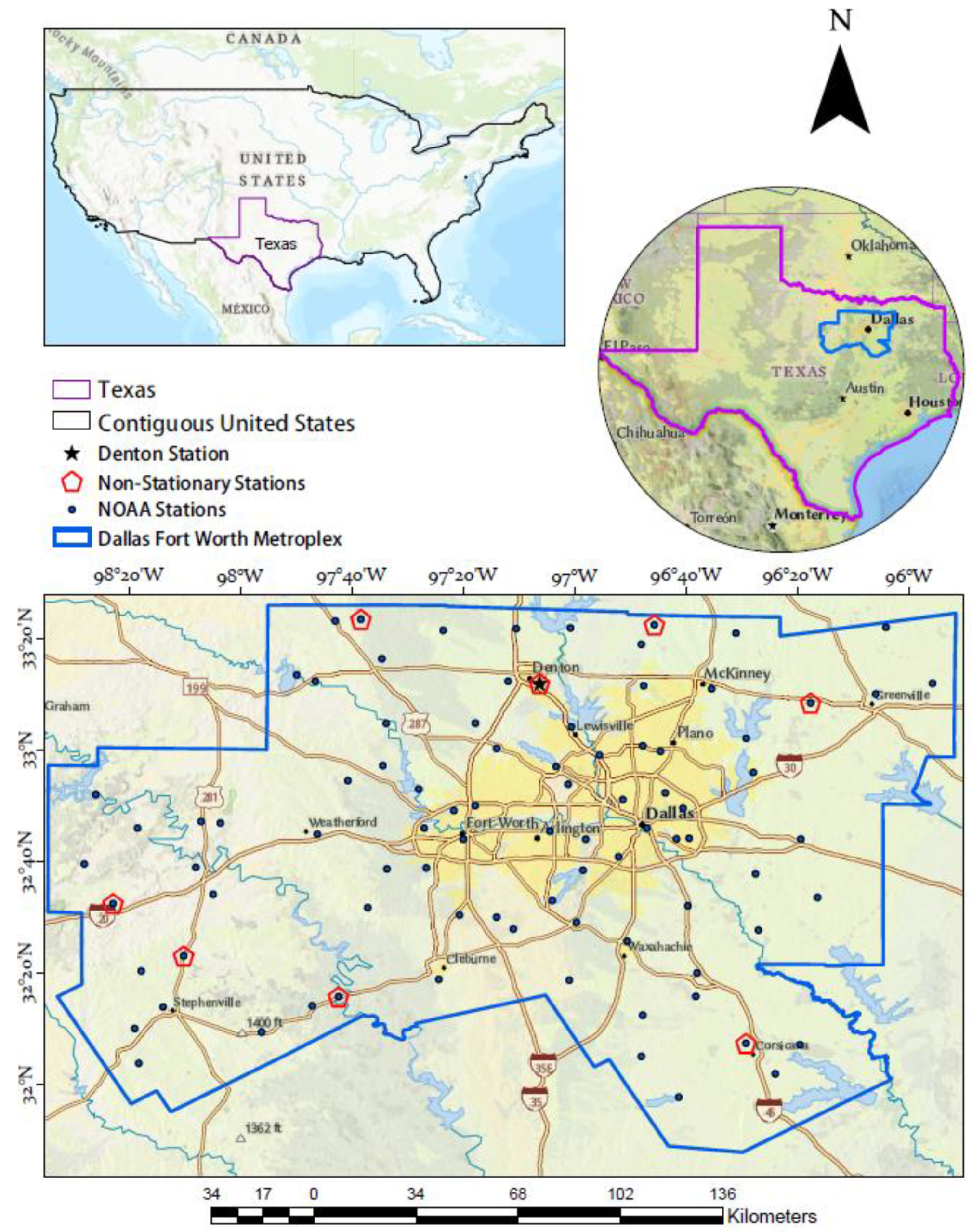
2.1. Study Area

The Dallas–Fort Worth (DFW) metropolitan area (Figure 1) lies in north central Texas, with 16 counties covering an area of 12,741 mi2 (~33,000 km2). It includes two major cities (Dallas and Fort Worth) and more than 100 smaller cities with a population of ~7.6 million (US Census Bureau’s 2020 census). Furthermore, by 2030, the population of DFW is projected to reach 9.1 million. Comparing the 1.52% population growth rate in the DFW area in 2021 with the 1.1% for Texas and 0.58% for the US, the DFW metroplex is one of the fastest-growing urban areas in the US. As a result, the urban development in DFW has increased, resulting in more impervious surfaces and vulnerability to flooding [30].
The DFW region, with an annual average rainfall of ~36 inches (914 mm), has flooded several times due to extreme precipitation. Between 1900 and 2010, there was an increase in average rainfall by 15% in the region [31]. In particular, extreme storm events increased by ~7% between 1960 and 2020 [32]. For example, on 24 May 1986, Fort Worth, the 2nd-largest city in the DFW metroplex, received 3.5 inches (88.9 mm) of rainfall in an hour, causing flash flooding that cost 2 million USD in damages and caused two fatalities [33]. Since then, the DFW metroplex has experienced at least four notable extreme precipitation events. On 24 May 2014, three inches (76.2 mm) of precipitation fell within 90 min, leading to the flooding of roads and infrastructure. May 2015, with a monthly rainfall of 16.5 inches (419.1 mm) and a daily downpour of three inches on 24 May, was the wettest May on record. This unusually high storm event resulted in flooding and accrued an estimated 1 billion USD in insured losses of properties and public infrastructure. On 16 January 2020, 4 inches (101.6 mm) of precipitation fell within 24 h in the region, causing flash floods, and most recently, on 22 August 2022, some parts of DFW recorded > 13 inches (>330 mm) of rainfall in 24 h, which was equivalent to a 0.1% chance of happening in a year as they were in a 1000-year flood event [34]. Despite this, the IDF curves (Atlas 14) developed for this region are based on a stationary assumption. Therefore, they may not provide adequate information to plan for resilient infrastructures that can withstand non-stationary precipitation trends and projected increases resulting from climate change.

2.2. Data and Key Steps

This study used the daily AMS of the historical precipitation data used by NOAA to develop their IDF curves or Atlas 14 [18]. AMS data from 88 stations in the study area were extracted from the NOAA Precipitation Frequency Data Server (PFDS) via their web portal (https://hdsc.nws.noaa.gov) (Access date on 11 March 2022). The study methods and key steps are shown in Figure 2.
Key steps include:
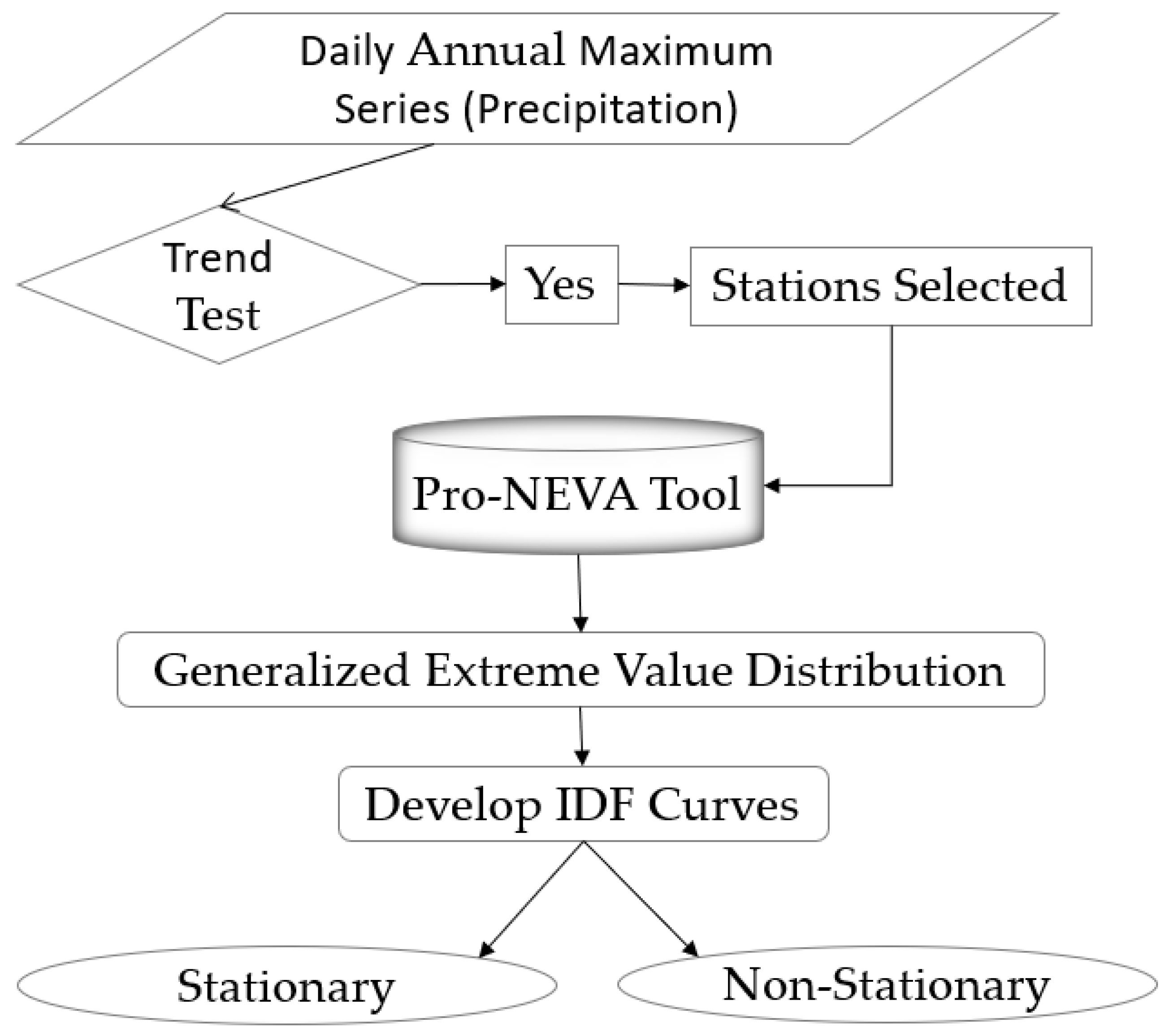
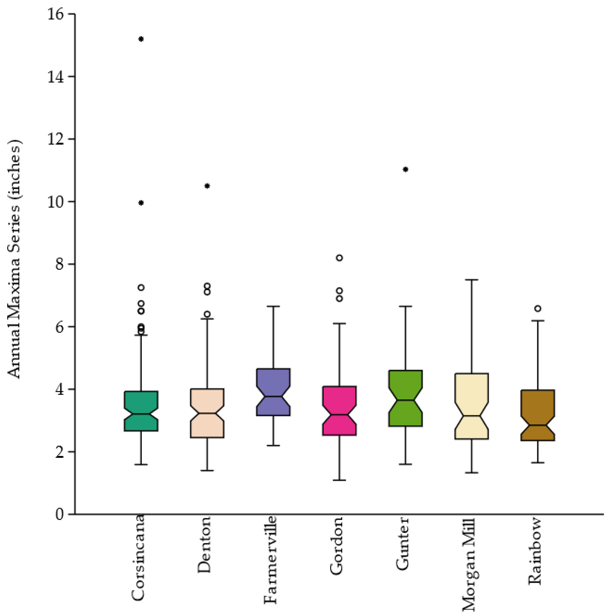
  • Following the methods of Atlas 14 [18], the daily duration the AMS data of 88 stations in the study area were used for developing historical IDF curves.
  • To determine whether the AMS data followed the stationary or non-stationary trend, two null-hypothesis significance trend tests, namely, Mann–Kendall (MK) [35] and Pettitt (PT) [36] used in hydrology and extreme analyses, were chosen. These two tests are popularly used and recommended in the hydrology and climate literature [29,37,38] for analyzing hydro-climatological time series data, including precipitation AMS [18]. Only those stations exhibiting a trend and change point detection were selected for developing IDF curves under non-stationary conditions.
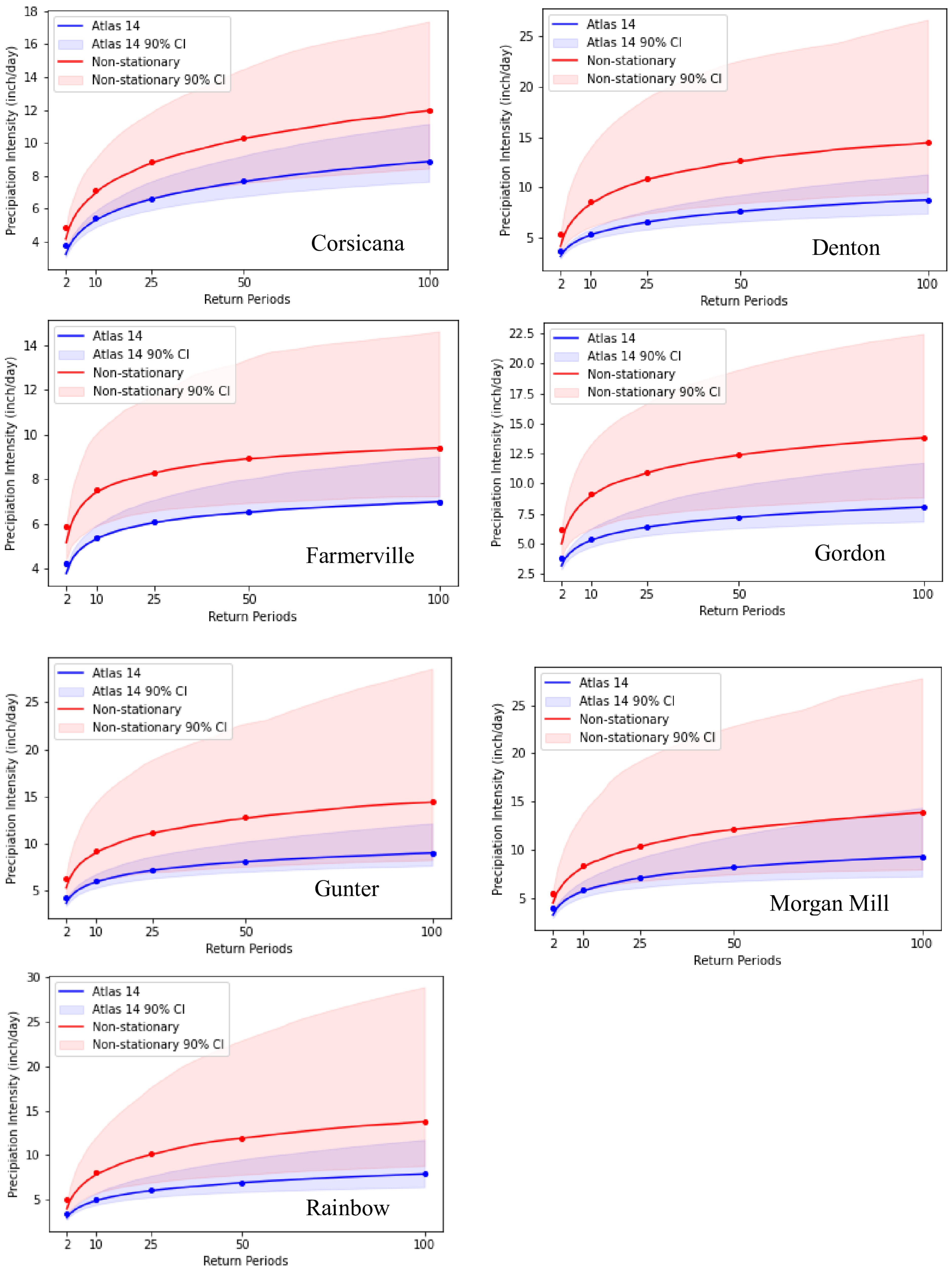
  • In this research, 24 h duration IDF curves were developed using Process-informed Non-stationary Extreme Value Analysis (ProNEVA) software (https://amir.eng.uci.edu/software.php#:~:text=Process%2Dinformed%20Nonstationary%20Extreme%20Value%20Analysis%20(ProNEVA)%20is%20a,change%20in%20statistics%20of%20extremes, accessed on 22 October 2023) [39], because a 24 h duration is one of the most commonly used durations for assessing rainfall intensity and designing drainage systems. It is also a duration of interest for flood management in many areas.
  • ProNEVA is a statistical modeling framework developed to estimate the frequency and magnitude of extreme events, such as floods and droughts, under stationary and non-stationary conditions. ProNEVA is a modified and the most recent version of the NEVA tool developed by Cheng et al. [25]. The GEV method was used for fitting the AMS distribution, as GEV is a commonly used distribution to model extreme events [40,41,42,43]. Moreover, NOAA used the GEV distribution function to develop Atlas 14. The GEV distribution had three parameters as explained by θ = (μ,σ,ξ), where the location parameter (μ) explains the center of the distribution, the scale parameter (σ) determines the size of deviations around the location parameter, and the shape parameter (ξ) governs the tail behavior of the GEV distribution. In this study, the location and scale parameters were assumed to be linear functions of time to account for non-stationarity while keeping the shape parameter constant, because the shape parameter is known to be difficult to precisely estimate, even in the stationary case [20,39]. Pro-NEVA uses the Bayes theorem for estimating GEV parameters under the non-stationary assumption. According to the Bayes theorem, the probability of an event occurring given some prior knowledge and new evidence is proportional to the product of the prior probability and the likelihood of the evidence given the event [44]. The Bayes approach is beneficial when there is incomplete or uncertain information and decisions must be based on probabilities [45]. It also offers uncertainty in the parameter estimates, yielding more realistic estimations [46]. Cheng et al. [25] provided detailed explanations of the application of the Bayes theorem in generating non-stationary IDF curves.
  • Non-stationary IDF curves were developed for stations (Figure 1) that showed a trend (step 2) using the historical AMS data for each station as used in Atlas 14 and applying the GEV distribution to be consistent with the method used in Atlas 14. As the ProNEVA tool uses the Bayes theorem for estimating the GEV, prior parameters’ (μ,σ,ξ) values were calculated for each station, as listed in Table 1, and were used to develop the IDF curves for each station. This study used time as a covariate for the non-stationary assumption.
  • The performance of non-stationary and stationary models was evaluated using four statistical indices—the Akaike Information Criterion (AIC), Bayesian Information Criterion (BIC), Root Mean Square Error (RMSE), and Nash–Sutcliffe Efficiency (NSE)—available in ProNEVA. AIC [47] and BIC [48] are probabilistic statistical measures to quantify model performance in hydro-climatological studies [49]. RMSE and NSE are the two most commonly used coefficients of the goodness of fit to select models based on minimum residual [50]. The selection of the final model in ProNEVA is based on the performance of the combination of all four statistical metrics—the AIC, BIC, RMSE, and NSE—that maximize the posterior distribution [39].
Then, the resulting IDF curves were compared to see if any differences could be observed in the intensity of storm events for a particular return period (e.g., a 24 h or 100-year storm event). For each station, the percentage change in the intensity of the extreme precipitation of the non-stationary-based IDF curves was calculated against Atlas 14 of the respective station. The fitted GEV distribution was sampled 10,000 times to obtain 10,000 estimates of a given rainfall depth for a given recurrence interval to indicate the uncertainty range at the 90% confidence interval.

3. Results

The results of the null hypothesis significant trend tests showed that, out of the 88 stations used in Atlas 14 for the DFW metroplex, Pettitt’s test showed a trend in twelve stations, and the MK test showed a trend in eight stations. Overall, seven stations (Corsicana, Denton, Farmersville, Gordon, Gunter, Morgan Mill, and Rainbow) showed a trend in Pettitt’s and MK tests statistically significant (p ≤ 0.05) as shown in Table A1. General statistical information about the annual maxima precipitation of these seven stations is presented in Figure A1 as a side-by-side box and whisker plot. Then, stationary and non-stationary IDF curves were developed for these seven stations. The non-stationary model was more successful than the stationary model at most stations. The lower AIC and BIC values, as well as lower RMSE values and higher NSE values for the non-stationary model (Table 1), suggested a better performance of non-stationary models over stationary models.
It was found that, with the stationary assumption, the rainfall intensities for all return periods (2-year, 10-year, 20-year, 50-year, and 100-year) were underestimated, as shown in Figure 3 and Table 2, representing the Corsicana, Denton, Farmersville, Gordon, Gunter, Morgan Hill, and Rainbow stations. For the Corsicana station, the 24 h rainfall intensity under the non-stationary condition increased by 30.8%, 32.7%, 33.3%, 34.2%, and 35.3% for the 2-year, 10-year, 20-year, 50-year, and 100-year periods, respectively, compared to the stationary Atlas 14. For the Denton station, the 24 h rainfall intensity under the non-stationary condition increased by 29.4%, 58.1%, 63.6%, 65.4%, and 65.4% for the 2-year, 10-year, 20-year, 50-year, and 100-year periods, respectively, compared to stationary Atlas 14. For the Farmersville station, the 24 h rainfall intensity under the non-stationary condition increased by 37.2%, 39.0%, 37.1%, 36.7%, and 34.5% for the 2-year, 10-year, 20-year, 50-year, and 100-year periods, respectively, compared to stationary Atlas 14. For the Gordon station, the 24 h rainfall intensity under the non-stationary condition increased by 55.5%, 69.9%, 70.1%, 71.3%, and 71.6% for the 2-year, 10-year, 20-year, 50-year, and 100-year periods, respectively, compared to stationary Atlas 14 (Figure 3). For the Gunter station, the 24 h rainfall intensity under the non-stationary condition increased by 43.8%, 53.3%, 55.9%, 57.1%, and 60.3% for the 2-year, 10-year, 20-year, 50-year, and 100-year periods, respectively, compared to stationary Atlas 14. For the Morgan Mill station, the 24 h rainfall intensity under the non-stationary condition increased by 41.9%, 44.2%, 45.8%, 49.2%, and 49.5% for the 2-year, 10-year, 20-year, 50-year, and 100-year periods, respectively, compared to stationary Atlas 14. For the Rainbow station, the 24 h rainfall intensity under the non-stationary condition increased by 33.7%, 58.9%, 65.5%, 71.9%, and 74.3% for the 2-year, 10-year, 20-year, 50-year, and 100-year periods, respectively, compared to stationary Atlas 14. For all stations except for Farmersville, there was a systematic underestimation of the 24 h precipitation intensity under the stationary condition from shorter to longer return periods by 14.6–120%.

4. Discussion

While most stations in the DFW region showed stationary trends with time, it is critical to acknowledge the non-stationarity behavior of other stations to assess the risks associated with extreme events, especially in the face of rapidly changing climatic conditions. Ignoring potential risks may prove costly to coupled human–natural systems [51,52]. For instance, Underwood et al. [53] stated that non-stationary precipitation events (e.g., due to the changing climate) could add roughly 22 to 36 billion USD in transportation and other infrastructure costs related to pavement maintenance and new construction in the US by 2070. Further, required mitigation measures and damages associated with a non-stationary climate are often exacerbated by growing and unsustainable urban growth; therefore, assessment studies should not discount low-probability events [54,55,56].
It is difficult, yet critical, to isolate the reasons for the non-stationary behavior of these seven stations (Figure 1) without further research. Climatic and hydrological data analysis techniques, such as the MK and Pettit tests, have been extensively explored in the scientific literature. Nonetheless, these tests present some differences, as underscored by Gholami et al. [57]. While the MK test might not have a high sensitivity toward sudden changes, the Pettit test can detect them [58]. These abrupt changes may arise from several sources, including but not limited to climate regime shifts, anthropogenic activities such as the construction of dam and reservoir systems, changes in land coverage and use, agricultural practices, river water displacement, the relocation of meteorological stations, alterations in variable calculation methods and observation time, or the modification of large-scale atmospheric circulation [59,60,61,62,63,64,65].
However, some potential reasons related to stations’ locations, physical environments, landforms, vegetation, and rural–urban fringe-creating unique microclimates might offer some insights. The Corsicana station, located on the southeastern side of the DFW metroplex, displayed non-stationarity. One potential reason for this trend could be a usually increasing west–east precipitation gradient in Texas and the US [22]. Moreover, Corsicana is located in a low-lying area with numerous creeks and streams and is surrounded by larger water bodies such as Richland-Chambers Reservoir, Navarro Mills Lake, and Lake Bardwell [66]. These water bodies, along with varied landscapes, could have created a microclimate contributing to the non-stationary trend. However, other nearby stations with water bodies in their periphery did not display a non-stationary trend, indicating the influence of other factors for the non-stationary trend.
One such factor could be the highly urbanized location of Corsicana. According to Liu and Niyogi [67], urbanization modifies the rainfall amount and intensity within different areas of a city, resulting in an increase in the mean precipitation downwind of the city by 18%, over the city by 16%, and on the left and right of the city by 2% and 4%, respectively. Potential changes in rainfall patterns in urban areas [68] could be attributed to the interaction of factors such as aerosol emissions, surface roughness, and heat storage [69]. The Denton station is situated in an urbanized area close to Lewisville Lake. Additionally, it has a diverse topography with rolling hills. Most likely, the local topography, the large lake effect, and its urban growth could be potential contributing factors to the observed non-stationary trend. Some studies have suggested that location-specific topography and slopes that alter humidity, wind motion, and direction could affect local extreme precipitation variability [70,71]. The stations of Gordon, Rainbow, and Morgan Mill, situated in southwestern DFW, are adjacent to mountains on the western side (Clayton and Palo Pinto Mountains) and numerous streams and lakes on the eastern side, which may have added orographic effects and caused erratic and higher precipitation events [72]. Furthermore, issues related to the screening and quality control (correction of missing, underestimated, or erroneously recorded events) of the AMS data by NOAA [18] could also be a potential factor. NOAA used a combination of data sources (nearby gauges, storm reports, storm data, and radar data) to determine unconstrained 24 h annual maximum values for extreme events. Therefore, trend tests (stationary or non-stationary) may be subject to data mining and quality control methods.
With the non-stationary models, the benchmark 100-year return period showed an increase of 34.5 to 74.3%, and the most frequently occurring 2-year storm event indicated an increase of up to 55% compared to the Atlas 14. These findings in the DFW metroplex are consistent with studies in other metropolitan regions in the US and elsewhere. For example, a study conducted by Cheng and Aghakouchak [25] at White Sands National Monument Station, New Mexico, found that non-stationary IDF curves produced higher rainfall intensities than stationary IDF curves. The authors observed that the stationary assumption underestimated extreme precipitation by as much as 60% in a 2 h duration, 2-year return period rainfall, which could potentially increase the frequency of flood risks and infrastructure failure several folds. Another study conducted by Soumya et al. [73] in Kerala, India, found that non-stationary IDF curves had higher rainfall intensities than stationary IDF curves, with an increase in rainfall intensity of greater than 50% for the 100-year return period under a non-stationary assumption compared to that of a stationary assumption. Similarly, a study conducted in the metropolitan region of Ontario, Canada, revealed similar findings. The authors found that, for the return period of 50–100 years, the standard stationary-based IDF curves needed to be updated by 2 to 44% to reflect the increases associated with non-stationary-based IDF curves [74].
While incorporating non-stationary assumptions into IDF curve development provides benefits, some limitations should be considered. First, the consideration that non-stationary assumptions require more complex statistical approaches and modeling techniques than including stationary assumptions. Moreover, non-stationary assumptions may produce results with higher uncertainties when including GCM-based future climate scenarios with inherent GCM-specific and resolution-related uncertainties [75,76,77]. In contrast, stationary assumptions are more straightforward to apply than non-stationary assumptions, mainly because they do not need to account for changes in climate and weather patterns over time. Therefore, stationary assumptions may be appropriate in those cases limited by data availability and with evidence of no long-term climate change [78]. Unfortunately, the cost of stationarity assumptions can be pretty high and burdensome, as stationary IDF curves can lead to inaccurate estimates of extreme rainfall events in areas prone to long-term climate change, land-use change, and other meteorological factors [79]. Therefore, it is crucial to detect a trend in precipitation over time and space and consider local factors before deciding on the appropriate method for the IDF curve development.

Study Limitations and Research Direction

While time could be one of the covariates in the development of non-stationary IDF curves, as performed in several other studies [80,81,82] and this study, it has limitations. First, time as a covariate alone may not adequately capture the complex changes in the meteorological, hydrological, and environmental factors that can affect the intensity and frequency of extreme rainfall events [81]. Second, the precipitation time series data may only sometimes have a sufficient resolution to capture the fine-scale variations in extreme rainfall events. Third, changes in the urban and suburban landscape, such as land use and land cover changes, with a varying intensity of growth from mixed-use development to single-family homes to different sizes of open spaces, can affect the intensity and frequency of extreme rainfall events but cannot be adequately captured by time alone [79]. Fourth, the limited data availability (e.g., the lack of continuous hourly, sub-daily, and daily precipitation data for several decades) can pose a challenge in estimating non-stationary IDF curves using only time as a covariate [78].
However, the limitation of using time as the only covariate can be addressed using other essential covariates, such as temperature, humidity, greenhouse gas concentrations, urban extent, and ocean–atmosphere oscillations. Including these covariates could improve the accuracy of estimating the intensity and frequency of extreme rainfall events. Among these covariates, temperature is a crucial factor affecting extreme rainfall events’ amount and intensity. Warmer temperatures can increase the moisture-holding capacity of the atmosphere, leading to more intense rainfall events. Studies have demonstrated that incorporating temperature into non-stationary IDF curve development can improve the accuracy of estimates for extreme rainfall events [81,83]. Topography is another covariate that can significantly impact extreme rainfall events’ intensity and frequency. Steep slopes may experience more intense rainfall due to increased airflow and uplift convergence.
In contrast, flat terrain may experience more frequent but less intense rainfall due to slow runoff and longer water residence time in the soil [83]. Incorporating land use and land cover changes, such as urbanization or deforestation, into non-stationary IDF curve development can also help to account for differences in surface properties, such as the albedo effect, which can affect the intensity and frequency of extreme rainfall events [79,81]. Also, large-scale atmospheric circulation patterns, such as El Niño-Southern Oscillation (ENSO) or North Atlantic Oscillation (NAO), can influence the intensity and frequency of extreme rainfall events. Incorporating these patterns into non-stationary IDF curve development can help to capture the effects of climate variability and improve estimates for extreme rainfall events [84,85].
Using the covariates above and time can improve the accuracy of non-stationary IDF curve development and help to prepare planners for extreme events in rapidly growing and larger metropolitan areas like the DFW metroplex. Overall, non-stationary IDF curves can provide valuable information to planners in urban areas like DFW, helping them to better prepare for and respond to extreme rainfall events. However, although our research findings are consistent with several studies conducted in different regions, caution should be exercised when interpreting these results. It is recommended that further research, particularly the use of other covariates and the use of the recently released CMIP-6 climate projections with robust downscaling and bias correction methods, and the development of IDF curves at different durations (sub-hourly and sub-daily, etc.), can be used to better understand the implications of these findings for flood risk management in the DFW metroplex.

5. Conclusions

The DFW metroplex is in a region prone to frequent severe thunderstorms and flash floods, with many communities and infrastructure systems being vulnerable to these extreme events. Our study revealed a non-stationary trend in seven stations’ long-term precipitation AMS in the DFW metroplex. Non-stationarity in these stations could be attributed to factors related to differences in localized microclimate, land uses, and topographic variations. The currently available IDF curves for the region do not consider this non-stationarity and, therefore, show an underestimation of precipitation intensities. The consequences of this kind of underestimation could be quite severe when most of the infrastructure is designed based on traditional, stationary IDF curves. Using non-stationary IDF curves could capture local events and effects, making it possible to estimate the probability of extreme events in a changing climate. This information may help planners to prepare for extreme events by identifying areas and infrastructure systems vulnerable to flooding and developing mitigation measures and resilient systems such as flood control and early warning systems.

Supplementary Materials

The following supporting information can be downloaded at: https://www.mdpi.com/article/10.3390/hydrology10120229/s1, File S1: Raw data and python script.

Author Contributions

Conceptualization, B.G. and G.K.; methodology, G.K. and L.C.; software, B.G. and G.K.; validation, G.K., E.G., L.C. and B.G.; formal analysis, B.G.; investigation, G.K., B.G., L.C. and E.G.; resources, G.K. and L.C.; data curation, B.G. and G.K.; writing—original draft preparation, B.G.; writing—review and editing, G.K., E.G., L.C. and B.G.; visualization, B.G. and G.K.; supervision, G.K.; project administration, G.K.; funding acquisition, G.K. All authors have read and agreed to the published version of the manuscript.

Funding

This work was supported in part by a grant from the TCU Research and Creative Activities Fund (FY2023-2024 TCU). Publication charges for this article were supported by the TCU Library Open Access Fund. There was no additional external funding received for this study.

Data Availability Statement

Publicly available datasets were analyzed in this study. This data can be found here [https://hdsc.nws.noaa.gov] (Access date on 11 March 2022). The data and python scripts are available as Supplementary Material.

Conflicts of Interest

The authors declare no conflict of interest. The funders had no role in the design of the study; in the collection, analyses, or interpretation of data; in the writing of the manuscript; or in the decision to publish the results.

Appendix A

Table A1. Results of the Mann–Kendall and Pettit’s tests at the 0.05 significance level.
StationMann–Kendall TestPettit’s Test
p-Valuez-Statisticp-ValueU-Statistic
Corsicana0.00392.88600.00181299
Denton0.01852.35600.00171067
Farmerville0.00442.84900.0179313
Gordon0.00642.72870.0170453
Gunter0.02892.18490.0246295
Morgan Mill0.02372.26170.0308347
Rainbow0.01242.49900.0229560
Figure A1. A side-by-side box and whisker plot showing annual maxima precipitation for seven stations. Circles and stars indicate outliers outside 1.5 and 3.0 times the interquartile range, respectively.
Hydrology 10 00229 g0a1

References

  1. NOAA. Climate at a Glance. Available online: https://www.ncei.noaa.gov/access/monitoring/climate-at-a-glance/ (accessed on 14 January 2023).
  2. Sarkar, S.; Maity, R. Global climate shift in 1970s causes a significant worldwide increase in precipitation extremes. Sci. Rep. 2021, 11, 11574. [Google Scholar] [CrossRef] [PubMed]
  3. Damberg, L.; AghaKouchak, A. Global trends and patterns of drought from space. Theor. Appl. Climatol. 2014, 117, 441–448. [Google Scholar] [CrossRef]
  4. Tabari, H. Climate change impact on flood and extreme precipitation increases with water availability. Sci. Rep. 2020, 10, 13768. [Google Scholar] [CrossRef] [PubMed]
  5. Fischer, E.M.; Knutti, R. Observed heavy precipitation increase confirms theory and early models. Nat. Clim. Chang. 2016, 6, 986–991. [Google Scholar] [CrossRef]
  6. Berg, P.; Moseley, C.; Haerter, J.O. Strong increase in convective precipitation in response to higher temperatures. Nat. Geosci. 2013, 6, 181–185. [Google Scholar] [CrossRef]
  7. Dewan, A. Germany’s Deadly Floods Were up to 9 Times More Likely Because of Climate Change, Study Estimates; CNN Newssource Sales, Inc.: Atlanta, GA, USA, 2021. [Google Scholar]
  8. Kreienkamp, F.; Philip, S.Y.; Tradowsky, J.S.; Kew, S.F.; Lorenz, P.; Arrighi, J.; Belleflamme, A.; Bettmann, T.; Caluwaerts, S.; Chan, S.C. Rapid Attribution of Heavy Rainfall Events Leading to the Severe Flooding in Western Europe during July 2021; World Weather Atribution: Location, UK, 2021. [Google Scholar]
  9. Luu, L.N.; Scussolini, P.; Kew, S.; Philip, S.; Hariadi, M.H.; Vautard, R.; Van Mai, K.; Van Vu, T.; Truong, K.B.; Otto, F.; et al. Attribution of typhoon-induced torrential precipitation in Central Vietnam, October 2020. Clim. Chang. 2021, 169, 24. [Google Scholar] [CrossRef]
  10. Allan, R.P.; Barlow, M.; Byrne, M.P.; Cherchi, A.; Douville, H.; Fowler, H.J.; Gan, T.Y.; Pendergrass, A.G.; Rosenfeld, D.; Swann, A.L.S.; et al. Advances in understanding large-scale responses of the water cycle to climate change. Ann. N. Y. Acad. Sci. 2020, 1472, 49–75. [Google Scholar] [CrossRef]
  11. Walsh, J.; Wuebbles, D.; Hayhoe, K.; Kossin, J.; Kunkel, K.; Stephens, G.; Thorne, P.; Vose, R.; Wehner, M.; Willis, J.C. 2: Our changing climate. In Climate Change Impacts in the United States: The Third National Climate Assessment; U.S. Global Change Research Program: Washington, DC, USA, 2014; pp. 19–67. [Google Scholar]
  12. NOAA. US Billion-Dollar Weather and Climate Disasters. 2023. Available online: https://www.doi.org/10.25921/stkw-7w73 (accessed on 23 June 2023).
  13. Paul, S.; Ghebreyesus, D.; Sharif, H.O. Brief Communication: Analysis of the Fatalities and Socio-Economic Impacts Caused by Hurricane Florence. Geosciences 2019, 9, 58. [Google Scholar] [CrossRef]
  14. Bernard, M.M. Formulas for rainfall intensities of long duration. Trans. Am. Soc. Civ. Eng. 1932, 96, 592–606. [Google Scholar] [CrossRef]
  15. Hershfield, D.M. Rainfall Frequency Atlas of the United States; Technical Paper; US Dept of Commerce National Oceanic and Atmospheric Administration National Weather Service: Gray, ME, USA, 1961; Volume 40, pp. 1–61. [Google Scholar]
  16. NOAA. NOAA Updates Texas Rainfall Frequency Values: Data Is Used in Infrastructure Design and Flood Risk Management. Available online: https://www.noaa.gov/media-release/noaa-updates-texas-rainfall-frequency-values (accessed on 14 November 2022).
  17. Miller, J.F.; Frederick, R.H.; Tracey, R.J. Precipitation-Frequency Atlas of the Western United States; Soil Conservation Service, Engineering, Division; U.S. Department of Commerce, National Oceanic and Atmospheric Administration, National Weather Service: Silver Spring, ML, USA, 1973. [Google Scholar]
  18. Perica, S.; Pavlovic, S.; Laurent, M.; Trypaluk, C.; Unruh, D.; Wilhite, O. Precipitation-Frequency Atlas of the United States, Texas; NOAA Atlas; NOAA, National Weather Service: Silver Spring, MD, USA, 2018; Volume 14. [Google Scholar]
  19. Tank, A.M.G.K.; Können, G.P. Trends in Indices of Daily Temperature and Precipitation Extremes in Europe, 1946–99. J. Clim. 2003, 16, 3665–3680. [Google Scholar] [CrossRef]
  20. Coles, S. An Introduction to Statistical Modeling of Extreme Values; Springer: London, UK, 2013. [Google Scholar]
  21. Alexander, L.V.; Zhang, X.; Peterson, T.C.; Caesar, J.; Gleason, B.; Klein Tank, A.M.G.; Haylock, M.; Collins, D.; Trewin, B.; Rahimzadeh, F.; et al. Global observed changes in daily climate extremes of temperature and precipitation. J. Geophys. Res.—Atmos. 2006, 111, D05109-n/a. [Google Scholar] [CrossRef]
  22. Easterling, D.R.; Arnold, J.; Knutson, T.; Kunkel, K.; LeGrande, A.; Leung, L.R.; Vose, R.; Waliser, D.; Wehner, M. Precipitation Change in the United States; NASA: Washington, DC, USA, 2017.
  23. Groisman, P.Y.; Knight, R.W.; Easterling, D.R.; Karl, T.R.; Hegerl, G.C.; Razuvaev, V.N. Trends in Intense Precipitation in the Climate Record. J. Clim. 2005, 18, 1326–1350. [Google Scholar] [CrossRef]
  24. Kunkel, K.E. North American trends in extreme precipitation. Nat. Hazards 2003, 29, 291–305. [Google Scholar] [CrossRef]
  25. Cheng, L.; AghaKouchak, A. Nonstationary precipitation intensity-duration-frequency curves for infrastructure design in a changing climate. Sci. Rep. 2014, 4, 7093. [Google Scholar] [CrossRef] [PubMed]
  26. Soulis, E.D.; Sarhadi, A.; Tinel, M.; Suthar, M. Extreme precipitation time trends in Ontario, 1960–2010. Hydrol. Process. 2016, 30, 4090–4100. [Google Scholar] [CrossRef]
  27. Wi, S.; Valdés, J.B.; Steinschneider, S.; Kim, T.-W. Non-stationary frequency analysis of extreme precipitation in South Korea using peaks-over-threshold and annual maxima. Stoch. Environ. Res. Risk Assess. 2016, 30, 583–606. [Google Scholar] [CrossRef]
  28. Cooley, D.; Nychka, D.; Naveau, P. Bayesian Spatial Modeling of Extreme Precipitation Return Levels. J. Am. Stat. Assoc. 2007, 102, 824–840. [Google Scholar] [CrossRef]
  29. Cheng, L.; AghaKouchak, A.; Gilleland, E.; Katz, R.W. Non-stationary extreme value analysis in a changing climate. Clim. Chang. 2014, 127, 353–369. [Google Scholar] [CrossRef]
  30. Feng, B.; Zhang, Y.; Bourke, R. Urbanization impacts on flood risks based on urban growth data and coupled flood models. Nat. Hazards 2021, 106, 613–627. [Google Scholar] [CrossRef]
  31. Winguth, A.; Lee, J.H.; Ko, Y. Climate Change/Extreme Weather Vulnerability and Risk Assessment for Transportation Infrastructure in Dallas and Tarrant Counties; University of Texas at Arlington: Arlington, TX, USA, 2015. [Google Scholar]
  32. Nielsen-Gammon, J.; Escobedo, J.; Ott, C.; Dedrick, J.; Van Fleet, A. Assessment of Historic and Future Trends of Extreme Weather in Texas, 1900–2036; Texas A&M University: College Station, TX, USA, 2020; p. 40. [Google Scholar]
  33. Lanning-Rush, J.; Asquith, W.H.; Slade, R.M., Jr. Extreme Precipitation Depths for Texas, Excluding the Trans-Pecos Region; U.S. Geological Survey: Austin, TX, USA, 1998. [Google Scholar]
  34. Dey, S.D.; Douglas, E. Flooding Hits Dallas-Fort Worth as Some Areas Receive More Than 13 Inches of Rain; The United Press International: Washington, DC, USA, 2022. [Google Scholar]
  35. Kendall, M.G. Rank Correlation Methods, 2nd ed.; Hafner Pub. Co.: New York, NY, USA, 1955. [Google Scholar]
  36. Pettitt, A.N. A Non-Parametric Approach to the Change-Point Problem. Appl. Stat. 1979, 28, 126–135. [Google Scholar] [CrossRef]
  37. Sam, M.G.; Nwaogazie, I.L.; Ikebude, C. Non-Stationary Trend Change Point Pattern Using 24-Hourly Annual Maximum Series (AMS) Precipitation Data. J. Water Resour. Prot. 2022, 14, 592–609. [Google Scholar] [CrossRef]
  38. Um, M.-J.; Heo, J.-H.; Markus, M.; Wuebbles, D.J. Performance Evaluation of four Statistical Tests for Trend and Non-stationarity and Assessment of Observed and Projected Annual Maximum Precipitation Series in Major United States Cities. Water Resour. Manag. 2018, 32, 913–933. [Google Scholar] [CrossRef]
  39. Ragno, E.; AghaKouchak, A.; Cheng, L.; Sadegh, M. A generalized framework for process-informed nonstationary extreme value analysis. Adv. Water Resour. 2019, 130, 270–282. [Google Scholar] [CrossRef]
  40. Hossain, I.; Khastagir, A.; Aktar, M.N.; Imteaz, M.A.; Huda, D.; Rasel, H.M. Comparison of estimation techniques for generalised extreme value (GEV) distribution parameters: A case study with Tasmanian rainfall. Int. J. Environ. Sci. Technol. 2022, 19, 7737–7750. [Google Scholar] [CrossRef]
  41. Park, J.S.; Kang, H.S.; Lee, Y.S.; Kim, M.K. Changes in the extreme daily rainfall in South Korea. Int. J. Climatol. 2011, 31, 2290–2299. [Google Scholar] [CrossRef]
  42. Rypkema, D.; Tuljapurkar, S. Modeling extreme climatic events using the generalized extreme value (GEV) distribution. In Handbook of Statistics; Elsevier: Amsterdam, The Netherlands, 2021; Volume 44, pp. 39–71. [Google Scholar]
  43. Zalina, M.D.; Desa, M.N.M.; Nguyen, V.T.V.; Kassim, A.H.M. Selecting a probability distribution for extreme rainfall series in Malaysia. Water Sci. Technol. 2002, 45, 63–68. [Google Scholar] [CrossRef]
  44. Swinburne, R. Bayes’ Theorem; Oxford University Press: Oxford, UK; New York, NY, USA, 2004; Volume 194, pp. 250–251. [Google Scholar]
  45. Barber, D. Bayesian Reasoning and Machine Learning; Cambridge University Press: Cambridge, UK, 2012. [Google Scholar]
  46. Robert, C.P. The Bayesian Choice: From Decision-Theoretic Foundations to Computational Implementation; Springer: New York, NY, USA, 2007. [Google Scholar]
  47. Akaike, H. A new look at the statistical model identification. IEEE Trans. Autom. Control 1974, 19, 716–723. [Google Scholar] [CrossRef]
  48. Schwarz, G. Estimating the Dimension of a Model. Ann. Stat. 1978, 6, 461–464. [Google Scholar] [CrossRef]
  49. Aho, K.; Derryberry, D.; Peterson, T. Model selection for ecologists: The worldviews of AIC and BIC. Ecology 2014, 95, 631–636. [Google Scholar] [CrossRef] [PubMed]
  50. Sadegh, M.; Moftakhari, H.; Gupta, H.V.; Ragno, E.; Mazdiyasni, O.; Sanders, B.; Matthew, R.; AghaKouchak, A. Multihazard Scenarios for Analysis of Compound Extreme Events. Geophys. Res. Lett. 2018, 45, 5470–5480. [Google Scholar] [CrossRef]
  51. Markolf, S.A.; Chester, M.V.; Helmrich, A.M.; Shannon, K. Re-imagining design storm criteria for the challenges of the 21st century. Cities 2021, 109, 102981. [Google Scholar] [CrossRef]
  52. Ren, H.; Hou, Z.J.; Wigmosta, M.; Liu, Y.; Leung, L.R. Impacts of Spatial Heterogeneity and Temporal Non-Stationarity on Intensity-Duration-Frequency Estimates-A Case Study in a Mountainous California-Nevada Watershed. Water 2019, 11, 1296. [Google Scholar] [CrossRef]
  53. Underwood, B.S.; Guido, Z.; Gudipudi, P.; Feinberg, Y. Increased costs to US pavement infrastructure from future temperature rise. Nat. Clim. Chang. 2017, 7, 704–707. [Google Scholar] [CrossRef]
  54. Chen, X.; Zhang, H.; Chen, W.; Huang, G. Urbanization and climate change impacts on future flood risk in the Pearl River Delta under shared socioeconomic pathways. Sci. Total Environ. 2021, 762, 143144. [Google Scholar] [CrossRef]
  55. Sterzel, T.; Luedeke, M.K.B.; Walther, C.; Kok, M.T.; Sietz, D.; Lucas, P.L. Typology of coastal urban vulnerability under rapid urbanization. PLoS ONE 2020, 15, e0220936. [Google Scholar] [CrossRef] [PubMed]
  56. Zhou, Q.; Leng, G.; Su, J.; Ren, Y. Comparison of urbanization and climate change impacts on urban flood volumes: Importance of urban planning and drainage adaptation. Sci. Total Environ. 2019, 658, 24–33. [Google Scholar] [CrossRef]
  57. Gholami, H.; Moradi, Y.; Lotfirad, M.; Gandomi, M.A.; Bazgir, N.; Hajibehzad, M.S. Detection of abrupt shift and non-parametric analyses of trends in runoff time series in Dez River Basin. Water Sci. Technol. Water Supply 2022, 22, 1216–1230. [Google Scholar] [CrossRef]
  58. Wijngaard, J.B.; Klein Tank, A.M.G.; Können, G.P. Homogeneity of 20th century European daily temperature and precipitation series. Int. J. Climatol. 2003, 23, 679–692. [Google Scholar] [CrossRef]
  59. Alley, R.B.; Marotzke, J.; Nordhaus, W.D.; Overpeck, J.T.; Peteet, D.M.; Pielke, R.A.; Pierrehumbert, R.T.; Rhines, P.B.; Stocker, T.F.; Talley, L.D.; et al. Abrupt Climate Change. Sci. (Am. Assoc. Adv. Sci.) 2003, 299, 2005–2010. [Google Scholar] [CrossRef]
  60. Hare, S.R.; Mantua, N.J. Empirical evidence for North Pacific regime shifts in 1977 and 1989. Prog. Oceanogr. 2000, 47, 103–145. [Google Scholar] [CrossRef]
  61. Potter, K.W. Evidence for nonstationarity as a physical explanation of the Hurst Phenomenon. Water Resour. Res. 1976, 12, 1047–1052. [Google Scholar] [CrossRef]
  62. Potter, K.W. Annual precipitation in the northeast United States: Long memory, short memory, or no memory? Water Resour. Res. 1979, 15, 340–346. [Google Scholar] [CrossRef]
  63. Swanson, K.L.; Tsonis, A.A. Has the climate recently shifted? Geophys. Res. Lett. 2009, 36, L06711-n/a. [Google Scholar] [CrossRef]
  64. Villarini, G.; Smith, J.A.; Serinaldi, F.; Ntelekos, A.A. Analyses of seasonal and annual maximum daily discharge records for central Europe. J. Hydrol. 2011, 399, 299–312. [Google Scholar] [CrossRef]
  65. Zuo, Q.; Guo, J.; Ma, J.; Cui, G.; Yang, R.; Yu, L. Assessment of regional-scale water resources carrying capacity based on fuzzy multiple attribute decision-making and scenario simulation. Ecol. Indic. 2021, 130, 108034. [Google Scholar] [CrossRef]
  66. Cox, S. A Developed Ideal Emergency Management Program Setting and Plan: A Case Study of Navarro County; Texas State University: San Marcos, TX, USA, 2006. [Google Scholar]
  67. Liu, J.; Niyogi, D. Meta-analysis of urbanization impact on rainfall modification. Sci. Rep. 2019, 9, 7301. [Google Scholar] [CrossRef]
  68. Patra, S.; Sahoo, S.; Mishra, P.; Mahapatra, S.C. Impacts of urbanization on land use/cover changes and its probable implications on local climate and groundwater level. J. Urban Manag. 2018, 7, 70–84. [Google Scholar] [CrossRef]
  69. Song, X.; Mo, Y.; Xuan, Y.; Wang, Q.J.; Wu, W.; Zhang, J.; Zou, X. Impacts of urbanization on precipitation patterns in the greater Beijing-Tianjin-Hebei metropolitan region in northern China. Environ. Res. Lett. 2021, 16, 14042. [Google Scholar] [CrossRef]
  70. Li, X.; Hu, Q. Spatiotemporal Changes in Extreme Precipitation and Its Dependence on Topography over the Poyang Lake Basin, China. Adv. Meteorol. 2019, 2019, 1253932. [Google Scholar] [CrossRef]
  71. Zhao, Y.; Chen, D.; Li, J.; Chen, D.; Chang, Y.; Li, J.; Qin, R. Enhancement of the summer extreme precipitation over North China by interactions between moisture convergence and topographic settings. Clim. Dyn. 2020, 54, 2713–2730. [Google Scholar] [CrossRef]
  72. Marra, F.; Armon, M.; Morin, E. Coastal and orographic effects on extreme precipitation revealed by weather radar observations. Hydrol. Earth Syst. Sci. 2022, 26, 1439–1458. [Google Scholar] [CrossRef]
  73. Soumya, R.; Anjitha, U.G.; Mohan, S.; Adarsh, S.; Gopakumar, R. Incorporation of non-stationarity in precipitation intensity-duration-frequency curves for Kerala, India. IOP Conf. Ser. Earth Environ. Sci. 2020, 491, 12013. [Google Scholar] [CrossRef]
  74. Ganguli, P.; Coulibaly, P. Does nonstationarity in rainfall require nonstationary intensity–duration–frequency curves? Hydrol. Earth Syst. Sci. 2017, 21, 6461–6483. [Google Scholar] [CrossRef]
  75. Agilan, V.; Umamahesh, N. Covariate and parameter uncertainty in non-stationary rainfall IDF curve. Int. J. Climatol. 2018, 38, 365–383. [Google Scholar] [CrossRef]
  76. Ragno, E.; AghaKouchak, A.; Love, C.A.; Cheng, L.; Vahedifard, F.; Lima, C.H.R. Quantifying Changes in Future Intensity-Duration-Frequency Curves Using Multimodel Ensemble Simulations. Water Resour. Res. 2018, 54, 1751–1764. [Google Scholar] [CrossRef]
  77. Silva, D.F.; Simonovic, S.P.; Schardong, A.; Goldenfum, J.A. Assessment of non-stationary IDF curves under a changing climate: Case study of different climatic zones in Canada. J. Hydrol. Reg. Stud. 2021, 36, 100870. [Google Scholar] [CrossRef]
  78. Chandra, R.; Saha, U.; Mujumdar, P. Model and parameter uncertainty in IDF relationships under climate change. Adv. Water Resour. 2015, 79, 127–139. [Google Scholar] [CrossRef]
  79. Singh, J.; Karmakar, S.; PaiMazumder, D.; Ghosh, S.; Niyogi, D. Urbanization alters rainfall extremes over the contiguous United States. Environ. Res. Lett. 2020, 15, 74033. [Google Scholar] [CrossRef]
  80. Agilan, V.; Umamahesh, N.V. Non-Stationary Rainfall Intensity-Duration-Frequency Relationship: A Comparison between Annual Maximum and Partial Duration Series. Water Resour. Manag. 2017, 31, 1825–1841. [Google Scholar] [CrossRef]
  81. Agilan, V.; Umamahesh, N.V. What are the best covariates for developing non-stationary rainfall Intensity-Duration-Frequency relationship? Adv. Water Resour. 2017, 101, 11–22. [Google Scholar] [CrossRef]
  82. Ouarda, T.B.M.J.; Yousef, L.A.; Charron, C. Non-stationary intensity-duration-frequency curves integrating information concerning teleconnections and climate change. Int. J. Climatol. 2019, 39, 2306–2323. [Google Scholar] [CrossRef]
  83. Roderick, T.P.; Wasko, C.; Sharma, A. An Improved Covariate for Projecting Future Rainfall Extremes? Water Resour. Res. 2020, 56, e2019WR026924. [Google Scholar] [CrossRef]
  84. Sun, Q.; Miao, C.; Qiao, Y.; Duan, Q. The nonstationary impact of local temperature changes and ENSO on extreme precipitation at the global scale. Clim. Dyn. 2017, 49, 4281–4292. [Google Scholar] [CrossRef]
  85. Whan, K.; Zwiers, F. The impact of ENSO and the NAO on extreme winter precipitation in North America in observations and regional climate models. Clim. Dyn. 2017, 48, 1401–1411. [Google Scholar] [CrossRef]
Figure 1. Dallas–Fort Worth metroplex (DFW) located in north central Texas, United States with precipitation stations (blue dots) and non-stationary-trend-exhibiting stations (red pentagons).
Hydrology 10 00229 g001
Figure 2. A schematic diagram showing study methodology and key steps.
Hydrology 10 00229 g002
Figure 3. Comparison between the non-stationary (red lines) and Atlas 14 (blue lines) at seven stations for one-day duration IDF curves, along with 90% confidence intervals for stationary (Atlas 14) and non-stationary models.
Hydrology 10 00229 g003
Table 1. Goodness of fit and model performance between stationary and non-stationary models for seven stations.
Stations ModelAkaike Information Criterion (AIC)Bayesian Information Criterion (BIC)Root Mean Square Error (RMSE)Nash–Sutcliffe Model Efficiency Coefficient (NSE)
CorsicanaStationary359.4367.73.150.95
Non-Stationary355.6369.42.440.97
DentonStationary329.0336.91.710.98
Non-Stationary325.9339.01.410.99
FarmersvilleStationary151.6157.41.520.97
Non-Stationary147.0156.71.580.97
GordonStationary221.1227.71.410.98
Non-Stationary216.4227.31.720.97
GunterStationary179.7185.52.380.94
Non-Stationary178.6188.32.790.92
Morgan MillStationary210.2216.31.610.97
Non-Stationary210.0220.32.370.95
RainbowStationary235.5242.51.850.97
Non-Stationary231.9243.71.530.98
Table 2. Difference between Atlas 14 (stationary) and non-stationary 24 h precipitation intensities for five return periods at seven stations in the Dallas–Fort Worth metroplex.
StationsPercentage Change (%) One-Day Precipitation Intensities at Five Return Levels
2-Year10-Year20-Year50-Year100-Year
Corsicana30.832.733.334.235.3
Denton29.458.163.665.465.4
Farmerville37.23937.136.734.5
Gordon55.569.970.171.371.6
Gunter43.853.355.957.160.3
Morgan Mill41.944.245.849.249.5
Rainbow 33.758.965.571.974.3
Disclaimer/Publisher’s Note: The statements, opinions and data contained in all publications are solely those of the individual author(s) and contributor(s) and not of MDPI and/or the editor(s). MDPI and/or the editor(s) disclaim responsibility for any injury to people or property resulting from any ideas, methods, instructions or products referred to in the content.

