
Differentiation of Multi-Parametric Groups of Groundwater Bodies through Discriminant Analysis and Machine Learning
 ,
,  , , , ,
Abstract
:1. Introduction
2. Materials and Methods
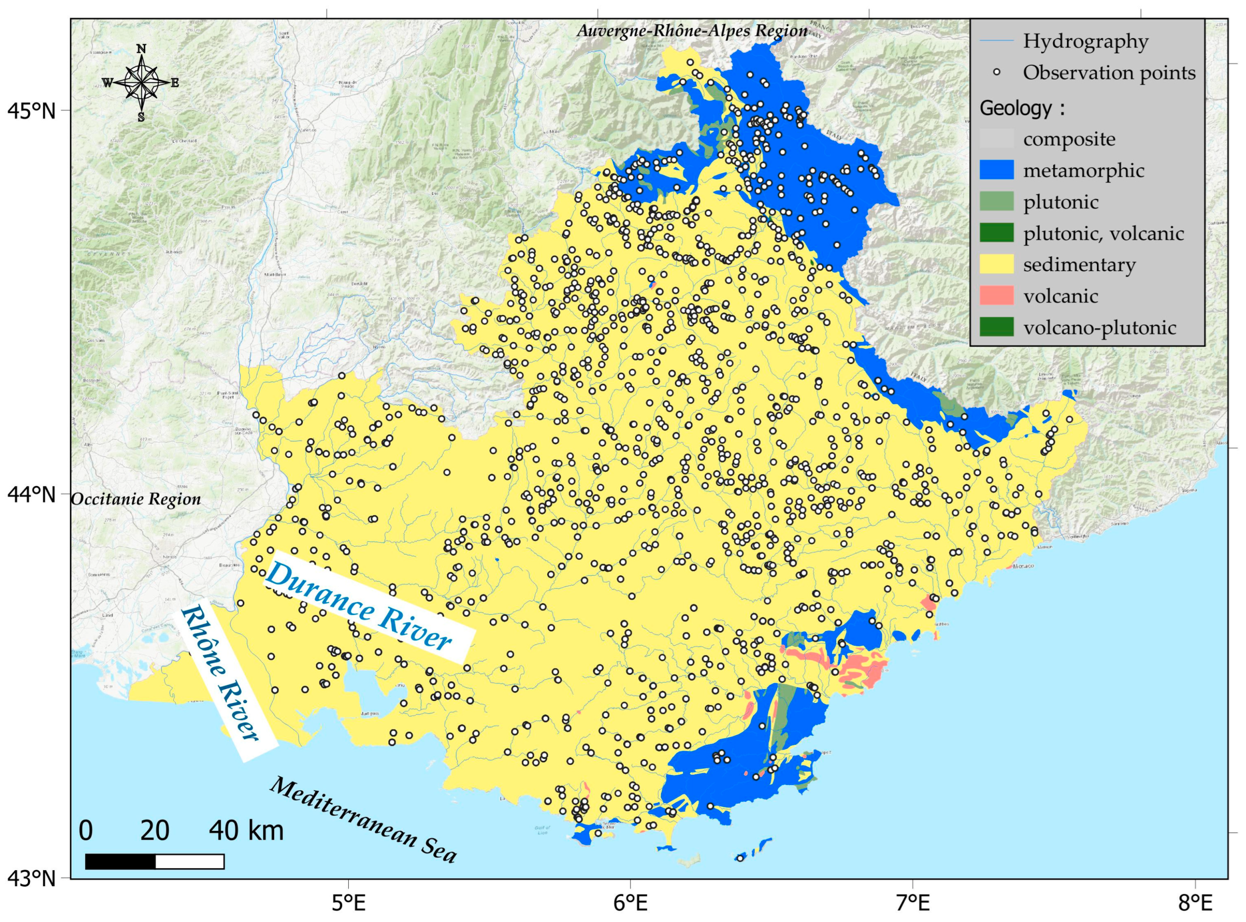
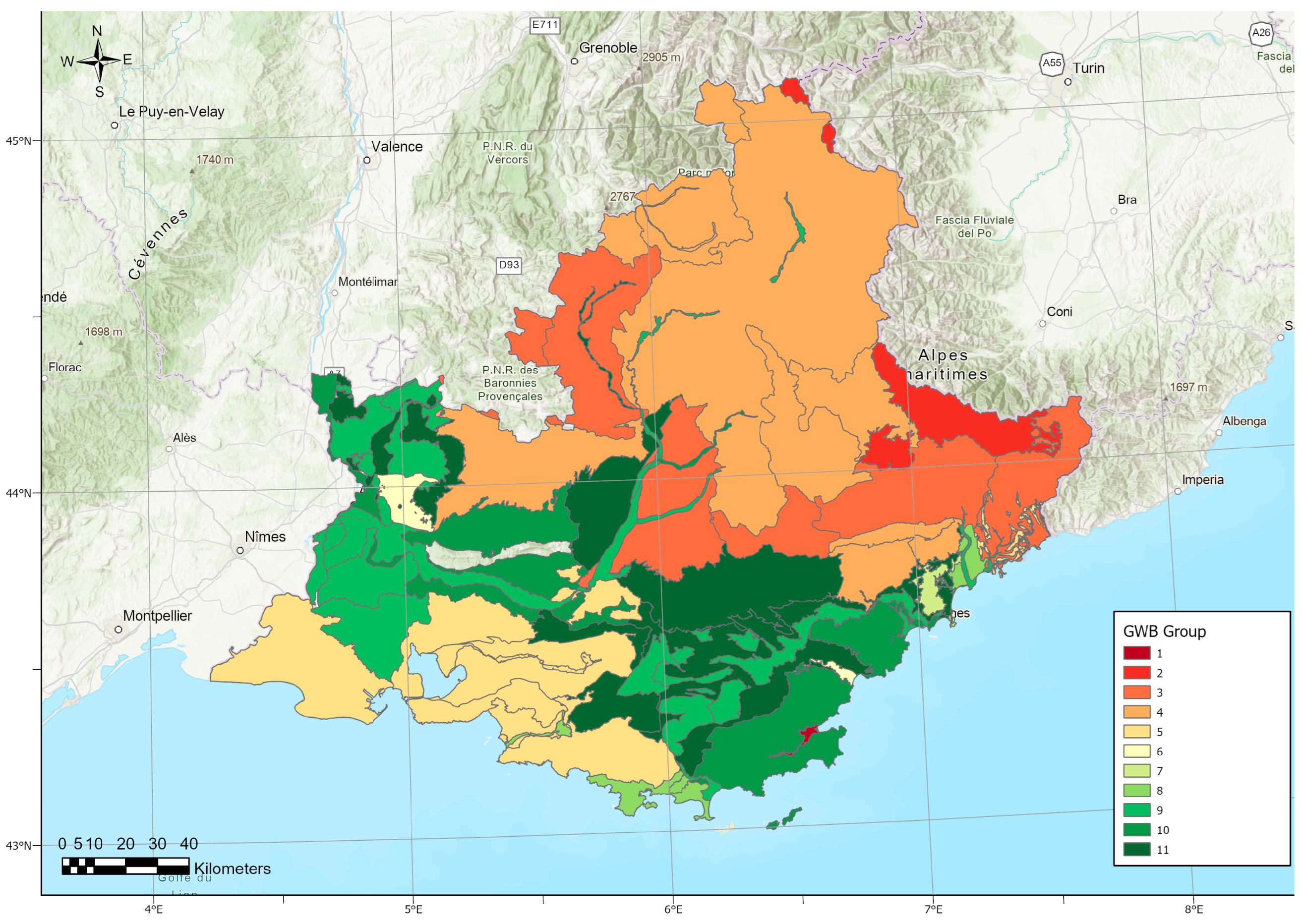
2.1. Study Area
2.2. SISE EAUX Database and Preliminary Processing
- Classical physico-chemical parameters (Electrical conductivity at 25 °C, pH, Total Dissolved Solids);
- Major ions (Ca2+, Mg2+, Na+, K+, HCO3−, SO42−, Cl−, NO3−) resulting from water-rock interactions and urban/agricultural pollution;
- Bacteriological parameters (Enterococcus, Escherichia coli), major indicators of faecal contamination.
- Trace elements such as metallic contaminants (Fe, Mn) sensitive to redox conditions, metalloids (As, B), and fluorine F.
2.3. Statistical and Machine Learning Methods
2.3.1. Discriminant Analysis Method
2.3.2. Machine Learning Methods
3. Results
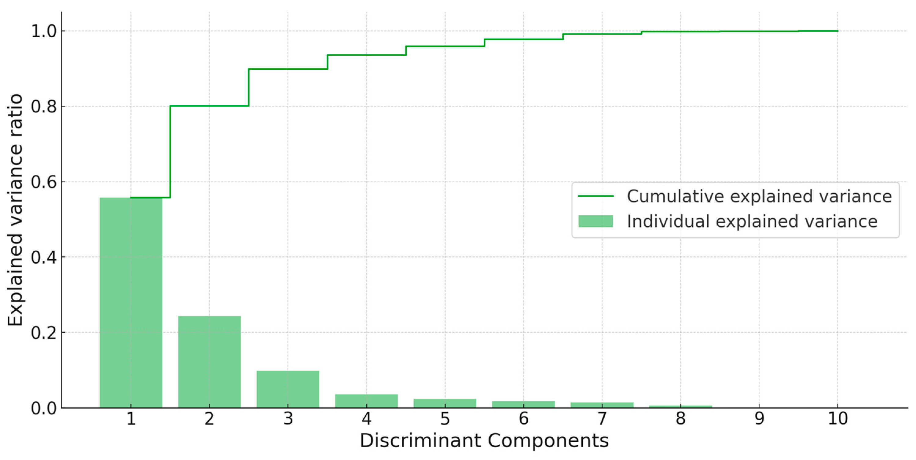
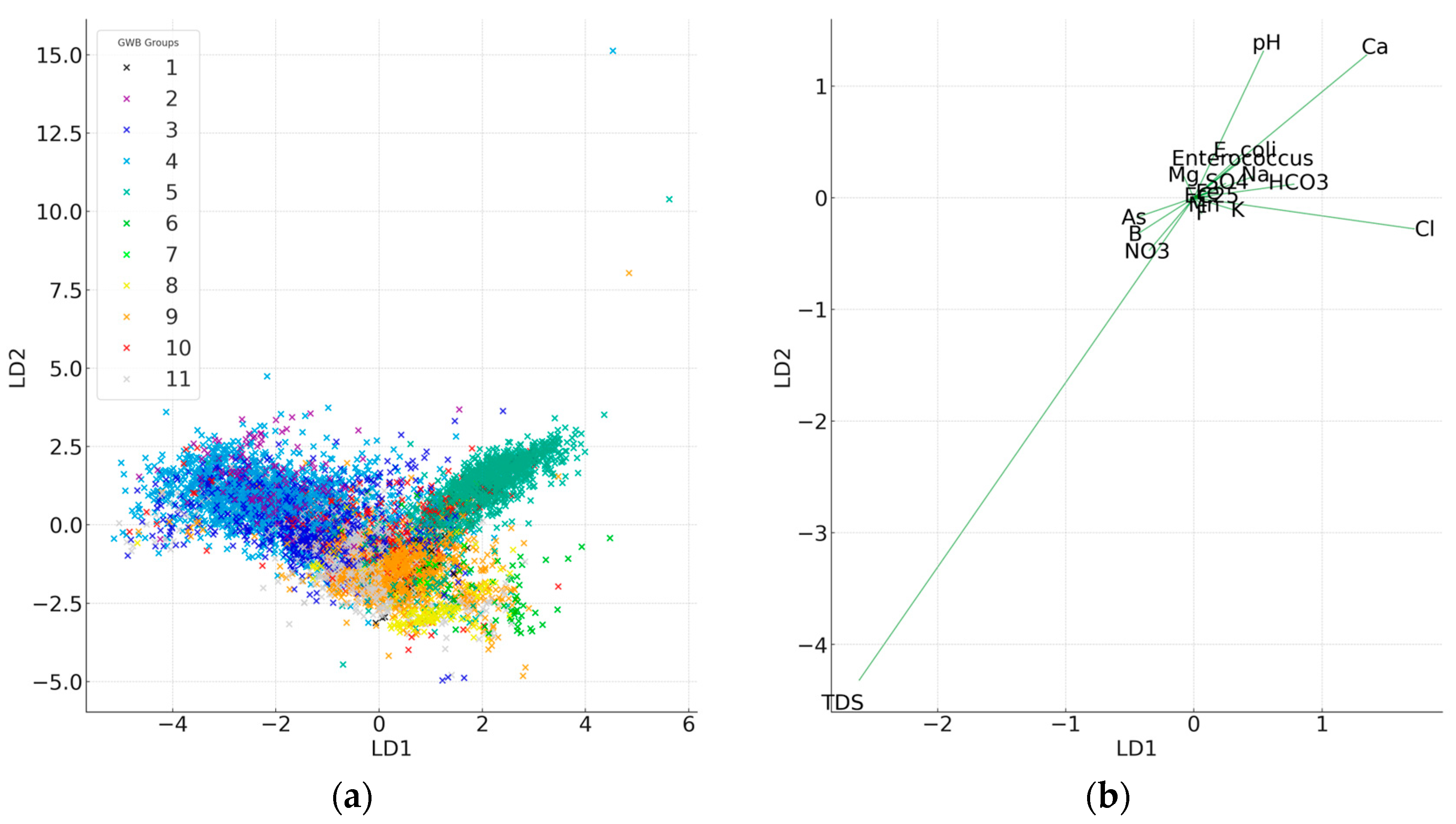
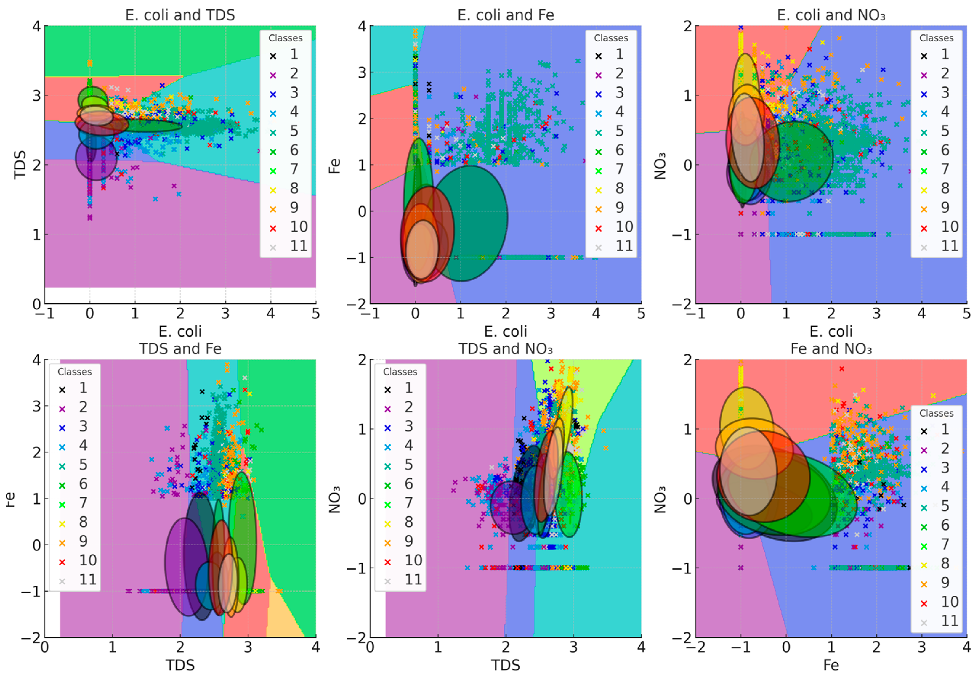
3.1. Discriminant Analysis
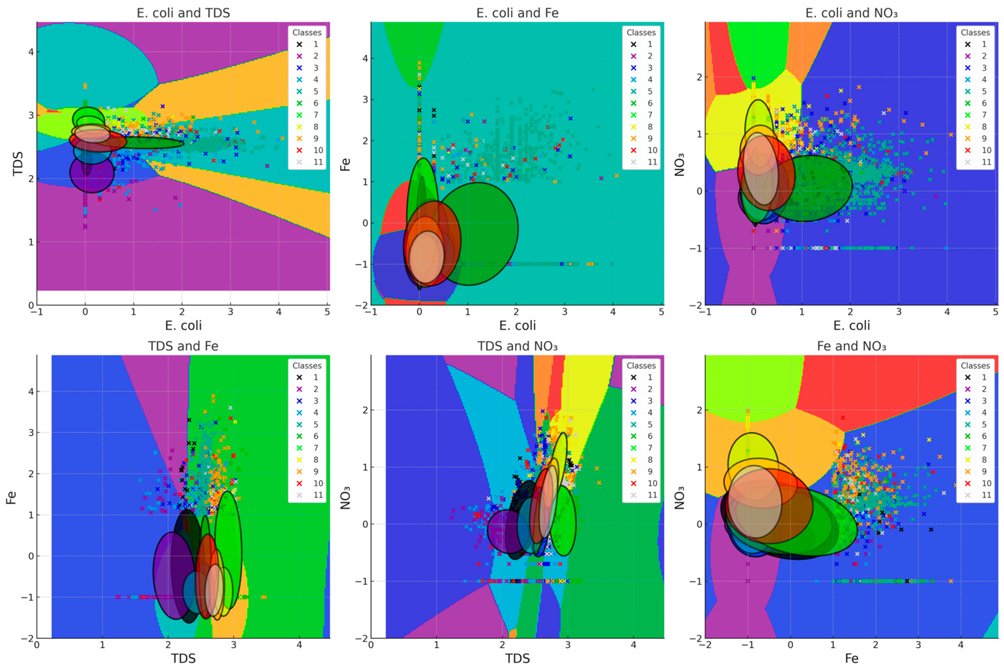
3.2. QDA Results
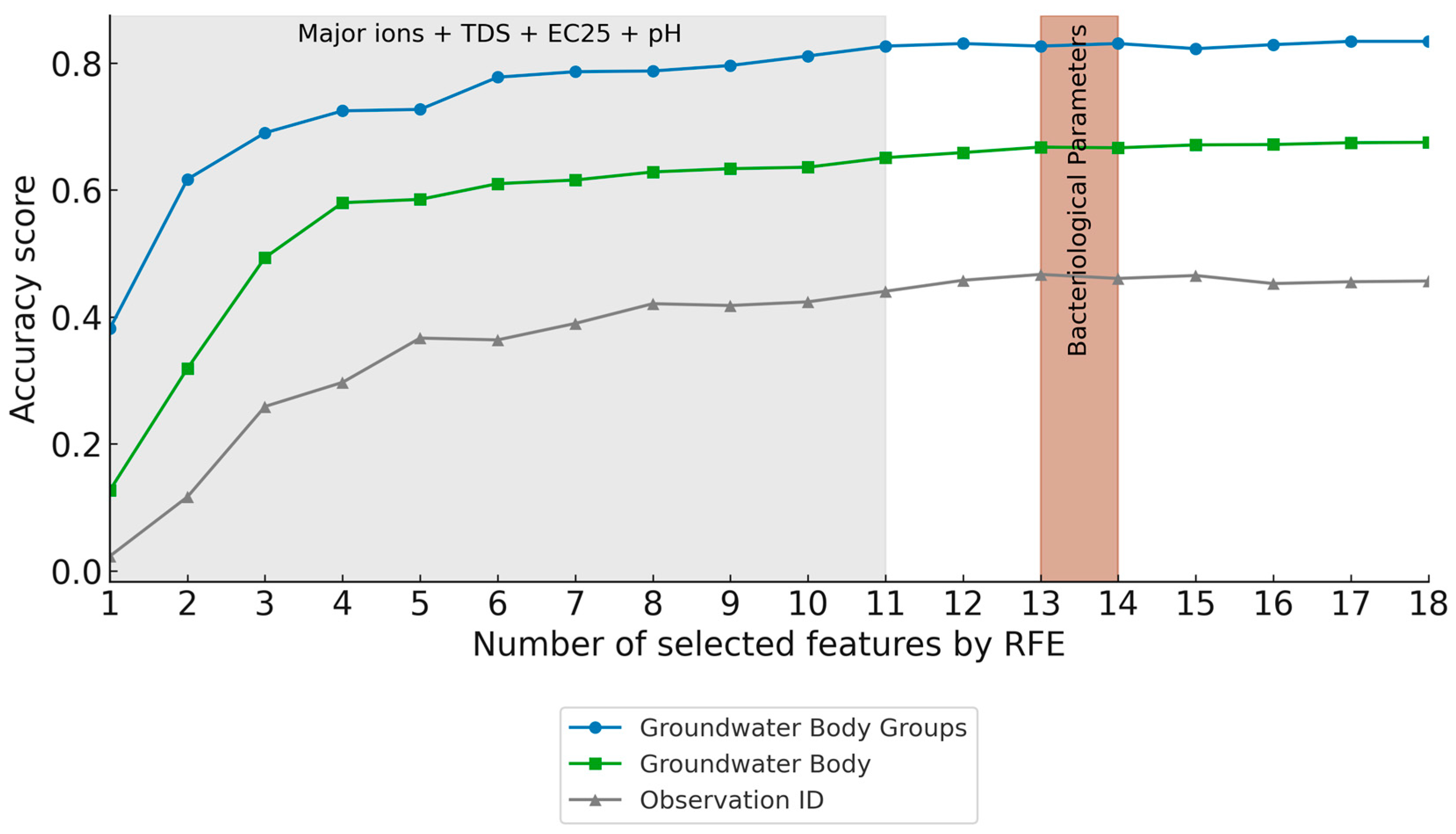
3.3. Machine Learning Based Methods
Feature Contribution
4. Discussion
4.1. Contrasting Water Quality
4.2. Disparities in Discrimination Depending on Parameters
5. Conclusions
Author Contributions
Funding
Data Availability Statement
Conflicts of Interest
References
- Korkka-Niemi, K. Cumulative Geological, Regional and Site-Specific Factors Affecting Groundwater Quality in Domestic Wells in Finland. Boreal Environ. Res. Monogr. 2001, 20, 1–20. [Google Scholar]
- Earman, S.; Dettinger, M. Potential Impacts of Climate Change on Groundwater Resources—A Global Review. J. Water Clim. Chang. 2011, 2, 213–229. [Google Scholar] [CrossRef]
- Barbieri, M.; Barberio, M.D.; Banzato, F.; Billi, A.; Boschetti, T.; Franchini, S.; Gori, F.; Petitta, M. Climate Change and Its Effect on Groundwater Quality. Environ. Geochem. Health 2023, 45, 1133–1144. [Google Scholar] [CrossRef] [PubMed]
- Lerner, D.N.; Harris, B. The Relationship between Land Use and Groundwater Resources and Quality. Land Use Policy 2009, 26, S265–S273. [Google Scholar] [CrossRef]
- Motlagh, A.M.; Yang, Z.; Saba, H. Groundwater Quality. Water Environ. Res. 2020, 92, 1649–1658. [Google Scholar] [CrossRef] [PubMed]
- Burri, N.M.; Weatherl, R.; Moeck, C.; Schirmer, M. A Review of Threats to Groundwater Quality in the Anthropocene. Sci. Total Environ. 2019, 684, 136–154. [Google Scholar] [CrossRef]
- European Commission Directive 2014/80/EU Amending Annex II to Directive 2006/118/EC of the European Parliament and of the Council on the Protection of Groundwater Against Pollution and Deterioration. Off. J. Eur. Union 2014, 52–55.
- European Commission Directive 2006/118/EC of the European Parliament and of the Council of 12 December 2006 on the Protection of Groundwater against Pollution and Deterioration. Off. J. Eur. Union 2006, 372, 19–31.
- European Commission Directive 2000/60/EC of the European Parliament and of the Council of 23 October 2000 Establishing a Framework for Community Action in the Field of Water Policy. Off. J. Eur. Communities 2000, 22, 2000.
- Allan, I.J.; Vrana, B.; Greenwood, R.; Mills, G.A.; Knutsson, J.; Holmberg, A.; Guigues, N.; Fouillac, A.-M.; Laschi, S. Strategic Monitoring for the European Water Framework Directive. TrAC Trends Anal. Chem. 2006, 25, 704–715. [Google Scholar] [CrossRef]
- Irish Working Group on Groundwater. Approach to Delineation of Groundwater Bodies, Guidance Document No.2. 2005. Available online: https://www.gsi.ie/documents/Groundwater%20Body%20Delineation.pdf (accessed on 28 November 2023).
- European Commission. Guidance Document No. 26. Guidance on Risk Assessment and the Use of Conceptual Models for Groundwater. 2010. Available online: https://op.europa.eu/en/publication-detail/-/publication/ab5b2e26-dabc-43aa-96ea-ef554b78eb09/language-en (accessed on 28 November 2023).
- European Commission. Guidance Document No. 22. Guidance on Implementing the Geographical Information System (GIS) Elements of the EU Water Policy. Tools and Services for Reporting under RBMP within WISE. Guidance on Reporting of Spatial Data for the WFD (RBMP); European Commission: Brussels, Belgium, 2009. [Google Scholar]
- European Commission. Guidance Document No 2: Identification of Water Bodies; European Commission: Brussels, Belgium, 2003. [Google Scholar]
- Duscher, K. Compilation of a Groundwater Body GIS Reference Layer. In Proceedings of the WISE GIS Workshop, Copenhagen, Denmark, 16–17 November 2010. [Google Scholar]
- Wendland, F.; Blum, A.; Coetsiers, M.; Gorova, R.; Griffioen, J.; Grima, J.; Hinsby, K.; Kunkel, R.; Marandi, A.; Melo, T.; et al. European Aquifer Typology: A Practical Framework for an Overview of Major Groundwater Composition at European Scale. Environ. Geol. 2008, 55, 77–85. [Google Scholar] [CrossRef]
- Tiouiouine, A.; Yameogo, S.; Valles, V.; Barbiero, L.; Dassonville, F.; Moulin, M.; Bouramtane, T.; Bahaj, T.; Morarech, M.; Kacimi, I. Dimension Reduction and Analysis of a 10-Year Physicochemical and Biological Water Database Applied to Water Resources Intended for Human Consumption in the Provence-Alpes-Cote d’azur Region, France. Water 2020, 12, 525. [Google Scholar] [CrossRef]
- Jabrane, M.; Touiouine, A.; Bouabdli, A.; Chakiri, S.; Mohsine, I.; Valles, V.; Barbiero, L. Data Conditioning Modes for the Study of Groundwater Resource Quality Using a Large Physico-Chemical and Bacteriological Database, Occitanie Region, France. Water 2022, 15, 84. [Google Scholar] [CrossRef]
- Lazar, H.; Ayach, M.; Barry, A.A.; Mohsine, I.; Touiouine, A.; Huneau, F.; Mori, C.; Garel, E.; Kacimi, I.; Valles, V.; et al. Groundwater Bodies in Corsica: A Critical Approach to GWBs Subdivision Based on Multivariate Water Quality Criteria. Hydrology 2023, 10, 213. [Google Scholar] [CrossRef]
- Tiouiouine, A.; Jabrane, M.; Kacimi, I.; Morarech, M.; Bouramtane, T.; Bahaj, T.; Yameogo, S.; Rezende-Filho, A.T.; Dassonville, F.; Moulin, M.; et al. Determining the Relevant Scale to Analyze the Quality of Regional Groundwater Resources While Combining Groundwater Bodies, Physicochemical and Biological Databases in Southeastern France. Water 2020, 12, 3476. [Google Scholar] [CrossRef]
- Mohsine, I.; Kacimi, I.; Abraham, S.; Valles, V.; Barbiero, L.; Dassonville, F.; Bahaj, T.; Kassou, N.; Touiouine, A.; Jabrane, M.; et al. Exploring Multiscale Variability in Groundwater Quality: A Comparative Analysis of Spatial and Temporal Patterns via Clustering. Water 2023, 15, 1603. [Google Scholar] [CrossRef]
- Jabrane, M.; Touiouine, A.; Valles, V.; Bouabdli, A.; Chakiri, S.; Mohsine, I.; El Jarjini, Y.; Morarech, M.; Duran, Y.; Barbiero, L. Search for a Relevant Scale to Optimize the Quality Monitoring of Groundwater Bodies in the Occitanie Region (France). Hydrology 2023, 10, 89. [Google Scholar] [CrossRef]
- Zhu, M.; Wang, J.; Yang, X.; Zhang, Y.; Zhang, L.; Ren, H.; Wu, B.; Ye, L. A Review of the Application of Machine Learning in Water Quality Evaluation. Eco-Environ. Health 2022, 1, 107–116. [Google Scholar] [CrossRef]
- He, S.; Wu, J.; Wang, D.; He, X. Predictive Modeling of Groundwater Nitrate Pollution and Evaluating Its Main Impact Factors Using Random Forest. Chemosphere 2022, 290, 133388. [Google Scholar] [CrossRef]
- Judeh, T.; Almasri, M.N.; Shadeed, S.M.; Bian, H.; Shahrour, I. Use of GIS, Statistics and Machine Learning for Groundwater Quality Management: Application to Nitrate Contamination. Water Resour. 2022, 49, 503–514. [Google Scholar] [CrossRef]
- Salem, S.B.H.; Gaagai, A.; Ben Slimene, I.; Ben Moussa, A.; Zouari, K.; Yadav, K.K.; Eid, M.H.; Abukhadra, M.R.; El-Sherbeeny, A.M.; Gad, M.; et al. Applying Multivariate Analysis and Machine Learning Approaches to Evaluating Groundwater Quality on the Kairouan Plain, Tunisia. Water 2023, 15, 3495. [Google Scholar] [CrossRef]
- Zounemat-Kermani, M.; Batelaan, O.; Fadaee, M.; Hinkelmann, R. Ensemble Machine Learning Paradigms in Hydrology: A Review. J. Hydrol. 2021, 598, 126266. [Google Scholar] [CrossRef]
- Haji-Aghajany, S.; Amerian, Y.; Amiri-Simkooei, A. Impact of Climate Change Parameters on Groundwater Level: Implications for Two Subsidence Regions in Iran Using Geodetic Observations and Artificial Neural Networks (ANN). Remote Sens. 2023, 15, 1555. [Google Scholar] [CrossRef]
- Lyons, K.J.; Ikonen, J.; Hokajärvi, A.-M.; Räsänen, T.; Pitkänen, T.; Kauppinen, A.; Kujala, K.; Rossi, P.M.; Miettinen, I.T. Monitoring Groundwater Quality with Real-Time Data, Stable Water Isotopes, and Microbial Community Analysis: A Comparison with Conventional Methods. Sci. Total Environ. 2023, 864, 161199. [Google Scholar] [CrossRef]
- Hastie, T.; Tibshirani, R.; Friedman, J. The Elements of Statistical Learning: Data Mining, Inference, and Prediction. 2009, Volume 2. Available online: https://link.springer.com/book/10.1007/978-0-387-84858-7 (accessed on 28 November 2023).
- Breiman, L. Random Forests. Mach. Learn. 2001, 45, 5–32. [Google Scholar] [CrossRef]
- Chen, T.; Guestrin, C. XGBoost: A Scalable Tree Boosting System. In Proceedings of the 22nd ACM SIGKDD International Conference on Knowledge Discovery and Data Mining, San Francisco, CA, USA, 13–17 August 2016; Association for Computing Machinery: New York, NY, USA, 2016; pp. 785–794. [Google Scholar]
- Quinlan, J.R. Induction of Decision Trees. Mach. Learn. 1986, 1, 81–106. [Google Scholar] [CrossRef]
- Schmidhuber, J. Deep Learning in Neural Networks: An Overview. Neural Netw. 2015, 61, 85–117. [Google Scholar] [CrossRef]
- Rish, I. An Empirical Study of the Naive Bayes Classifier. In Proceedings of the IJCAI 2001 Workshop on Empirical Methods in Artificial Intelligence, Seattle, WA, USA, 4–6 August 2001; pp. 41–46. [Google Scholar]
- Chery, L.; Laurent, A.; Vincent, B.; Tracol, R. Echanges SISE-Eaux/ADES: Identification Des Protocoles Compatibles Avec Les Scénarios d’échange SANDRE; Vincennes/Orléans, France. 2011. Available online: https://infoterre.brgm.fr/rapports/RP-59211-FR.pdf (accessed on 28 November 2023).
- Gran-Aymeric, L. Un Portail National Sur La Qualite Des Eaux Destinees a La Consommation Humaine. Tech. Sci. Méthodes 2010, 12, 45–48. [Google Scholar] [CrossRef]
- Pearson, K. LIII. On Lines and Planes of Closest Fit to Systems of Points in Space. Lond. Edinb. Dublin Philos. Mag. J. Sci. 1901, 2, 559–572. [Google Scholar] [CrossRef]
- Day, W.H.E.; Edelsbrunner, H. Efficient Algorithms for Agglomerative Hierarchical Clustering Methods. J. Classif. 1984, 1, 7–24. [Google Scholar] [CrossRef]
- Huberty, C.J. Discriminant Analysis. Rev. Educ. Res. 1975, 45, 543–598. [Google Scholar] [CrossRef]
- Ha, D.H.; Nguyen, P.T.; Costache, R.; Al-Ansari, N.; Van Phong, T.; Nguyen, H.D.; Amiri, M.; Sharma, R.; Prakash, I.; Van Le, H.; et al. Quadratic Discriminant Analysis Based Ensemble Machine Learning Models for Groundwater Potential Modeling and Mapping. Water Resour. Manag. 2021, 35, 4415–4433. [Google Scholar] [CrossRef]
- Singh, S.B.; Gupta, M.K.; Shukla, N.; Chaurasia, G.L.; Singh, S.; Tandon, P.K. Water purification: A brief review on tools and techniques used in analysis, monitoring and assessment of water quality. Green Chem. Technol. Lett. 2016, 2, 95–102. [Google Scholar] [CrossRef]
- Amiri, V.; Nakagawa, K. Using a Linear Discriminant Analysis (LDA)-Based Nomenclature System and Self-Organizing Maps (SOM) for Spatiotemporal Assessment of Groundwater Quality in a Coastal Aquifer. J. Hydrol. 2021, 603, 127082. [Google Scholar] [CrossRef]
- Wilson, S.R.; Close, M.E.; Abraham, P. Applying Linear Discriminant Analysis to Predict Groundwater Redox Conditions Conducive to Denitrification. J. Hydrol. 2018, 556, 611–624. [Google Scholar] [CrossRef]
- Ilić, I.; Puharić, M.; Ilić, D. Groundwater Quality Assessment and Prediction of Spatial Variations in the Area of the Danube River Basin (Serbia). Water Air Soil Pollut. 2021, 232, 117. [Google Scholar] [CrossRef]
- Ielpo, P.; Cassano, D.; Felice Uricchio, V.; Lopez, A.; Pappagallo, G.; Trizio, L.; de Gennaro, G. Identification of Pollution Sources and Classification of Apulia Region Groundwaters by Multivariate Statistical Methods and Neural Networks. Trans. ASABE 2013, 56, 1377–1386. [Google Scholar] [CrossRef]
- Sifaou, H.; Kammoun, A.; Alouini, M.-S. High-Dimensional Quadratic Discriminant Analysis Under Spiked Covariance Model. IEEE Access 2020, 8, 117313–117323. [Google Scholar] [CrossRef]
- DW Hosmer, D.J.; Lemeshow, S.; Sturdivant, R. Applied Logistic Regression; John Wiley & Sons: Hoboken, NJ, USA, 2013. [Google Scholar]
- Cover, T.; Hart, P. Nearest Neighbor Pattern Classification. IEEE Trans. Inf. Theory 1967, 13, 21–27. [Google Scholar] [CrossRef]
- Cortes, C.; Vapnik, V. Support-Vector Networks. Mach. Learn. 1995, 20, 273–297. [Google Scholar] [CrossRef]
- Schölkopf, B.; Smola, A. Learning with Kernels Support Vector Machines, Regularization, Optimization, and Beyond. 2002. Available online: https://direct.mit.edu/books/book/1821/Learning-with-KernelsSupport-Vector-Machines (accessed on 28 November 2023).
- Ke, G.; Meng, Q.; Finley, T.; Wang, T.; Chen, W.; Ma, W.; Ye, Q.; Liu, T.-Y. LightGBM: A Highly Efficient Gradient Boosting Decision Tree. In Proceedings of the Advances in Neural Information Processing Systems 30 (NIPS 2017), Long Beach, CA, USA, 4–9 December 2017; Guyon, I., Luxburg, U., Von Bengio, S., Wallach, H., Fergus, R., Vishwanathan, S., Garnett, R., Eds.; Curran Associates, Inc.: Red Hook, NY, USA, 2017; Volume 30. [Google Scholar]
- Ho, T.K. Nearest Neighbors in Random Subspaces. In Advances in Pattern Recognition; Amin, A., Dori, D., Pudil, P., Freeman, H., Eds.; Springer: Berlin/Heidelberg, Germany, 1998; pp. 640–648. [Google Scholar]
- Guyon, I.; Elisseeff, A. An Introduction to Variable and Feature Selection. J. Mach. Learn. Res. 2003, 3, 1157–1182. [Google Scholar]
- Li, F.; Yang, Y. Analysis of Recursive Feature Elimination Methods. In Proceedings of the 28th annual international ACM SIGIR Conference on Research and Development in Information Retrieval, Salvador, Brazil, 15–19 August 2005; ACM: New York, NY, USA, 2005; pp. 633–634. [Google Scholar]
- Strobl, C.; Boulesteix, A.-L.; Zeileis, A.; Hothorn, T. Bias in Random Forest Variable Importance Measures: Illustrations, Sources and a Solution. BMC Bioinform. 2007, 8, 25. [Google Scholar] [CrossRef] [PubMed]
- Baryannis, G.; Dani, S.; Antoniou, G. Predicting Supply Chain Risks Using Machine Learning: The Trade-off between Performance and Interpretability. Future Gener. Comput. Syst. 2019, 101, 993–1004. [Google Scholar] [CrossRef]
- Freitas, A.A. Automated Machine Learning for Studying the Trade-Off Between Predictive Accuracy and Interpretability. In Machine Learning and Knowledge Extraction; Holzinger, A., Kieseberg, P., Tjoa, A.M., Weippl, E., Eds.; Springer International Publishing: Cham, Switzerland, 2019; pp. 48–66. [Google Scholar]
- Dussart-Baptista, L. Transport Des Particules En Suspension et Des Bactéries Associées Dans l’aquifère Crayeux Karstique Haut-Normand. 2003. Available online: https://books.google.com.au/books/about/Transport_des_particules_en_suspension_e.html?id=paUEzgEACAAJ&hl=en&output=html_text&redir_esc=y (accessed on 28 November 2023).


| GWB Groups | ||||||||||||
|---|---|---|---|---|---|---|---|---|---|---|---|---|
| 1 | 2 | 3 | 4 | 5 | 6 | 7 | 8 | 9 | 10 | 11 | % | |
| 1 | 6 | 0 | 0 | 0 | 0 | 0 | 0 | 0 | 2 | 0 | 0 | 75 |
| 2 | 2 | 12 | 1 | 6 | 2 | 0 | 0 | 0 | 0 | 0 | 0 | 52.2 |
| 3 | 0 | 4 | 70 | 53 | 9 | 0 | 0 | 0 | 13 | 1 | 15 | 42.4 |
| 4 | 0 | 32 | 45 | 307 | 18 | 1 | 0 | 0 | 24 | 4 | 8 | 69.9 |
| 5 | 1 | 0 | 0 | 0 | 446 | 2 | 0 | 1 | 33 | 4 | 15 | 88.8 |
| 6 | 0 | 0 | 0 | 0 | 0 | 10 | 0 | 0 | 2 | 0 | 0 | 83.3 |
| 7 | 0 | 0 | 0 | 0 | 0 | 0 | 2 | 0 | 0 | 0 | 0 | 100 |
| 8 | 0 | 0 | 0 | 2 | 3 | 1 | 0 | 12 | 15 | 0 | 5 | 31.6 |
| 9 | 1 | 1 | 3 | 2 | 10 | 10 | 2 | 5 | 215 | 1 | 36 | 75.2 |
| 10 | 4 | 2 | 2 | 5 | 19 | 1 | 0 | 0 | 26 | 12 | 11 | 14.6 |
| 11 | 0 | 0 | 11 | 27 | 9 | 3 | 0 | 5 | 54 | 4 | 65 | 36.5 |
| GWB Groups | ||||||||||||
|---|---|---|---|---|---|---|---|---|---|---|---|---|
| 1 | 2 | 3 | 4 | 5 | 6 | 7 | 8 | 9 | 10 | 11 | % | |
| 1 | 2 | 0 | 0 | 0 | 0 | 0 | 0 | 1 | 1 | 4 | 0 | 25 |
| 2 | 0 | 16 | 2 | 3 | 0 | 0 | 0 | 0 | 0 | 2 | 0 | 70 |
| 3 | 0 | 3 | 122 | 14 | 7 | 0 | 0 | 2 | 11 | 4 | 2 | 74 |
| 4 | 0 | 23 | 173 | 185 | 3 | 0 | 0 | 2 | 36 | 7 | 10 | 42 |
| 5 | 1 | 0 | 1 | 3 | 455 | 0 | 0 | 10 | 24 | 6 | 2 | 91 |
| 6 | 0 | 0 | 0 | 0 | 0 | 9 | 0 | 0 | 3 | 0 | 0 | 75 |
| 7 | 0 | 0 | 0 | 0 | 2 | 0 | 0 | 0 | 0 | 0 | 0 | 0 |
| 8 | 0 | 0 | 2 | 0 | 3 | 0 | 0 | 27 | 5 | 1 | 0 | 71 |
| 9 | 0 | 1 | 10 | 2 | 30 | 3 | 0 | 55 | 172 | 6 | 7 | 60 |
| 10 | 0 | 2 | 5 | 2 | 28 | 1 | 0 | 1 | 18 | 21 | 4 | 26 |
| 11 | 0 | 0 | 32 | 11 | 7 | 3 | 0 | 28 | 76 | 8 | 13 | 7 |
| Classifier | Observation ID | GWB | GWB Groups |
|---|---|---|---|
| LDA | 0.41 | 0.40 | 0.67 |
| QDA | 0.001 | 0.17 | 0.59 |
| Classifier | Scale | ||
|---|---|---|---|
| Observation ID | GWB | GWB Groups | |
| Random Forest | 0.43 | 0.67 | 0.83 |
| Decision Tree | 0.26 | 0.49 | 0.74 |
| Neural Network | 0.33 | 0.46 | 0.71 |
| XGBoost | 0.34 | 0.57 | 0.75 |
| LightGBM | 0.09 | 0.14 | 0.80 |
| K-Nearest Neighbours | 0.20 | 0.48 | 0.73 |
| Ensemble (Subspace KNN) | 0.20 | 0.49 | 0.72 |
| Support Vector Machine | 0.22 | 0.42 | 0.68 |
| Kernal SVM | 0.05 | 0.33 | 0.66 |
| Logistic Regression | 0.14 | 0.39 | 0.65 |
| Gaussian Naive Bayes | 0.19 | 0.19 | 0.62 |
| Bernoulli Naive Bayes | 0.05 | 0.28 | 0.56 |
| Selected Features | |||||||||||||||||||
|---|---|---|---|---|---|---|---|---|---|---|---|---|---|---|---|---|---|---|---|
| TDS | Mg | SO4 | HCO3 | Na | Ca | Cl | NO3 | EC25 | pH | K | F | E. coli | Ent. | B | Fe | Mn | As | ||
| Total Number of Selected Parameters in RFE per iteration | 1 | 1 | |||||||||||||||||
| 2 | 0.57 | 0.43 | |||||||||||||||||
| 3 | 0.37 | 0.32 | 0.31 | ||||||||||||||||
| 4 | 0.26 | 0.26 | 0.24 | 0.24 | |||||||||||||||
| 5 | 0.21 | 0.21 | 0.2 | 0.19 | 0.19 | ||||||||||||||
| 6 | 0.17 | 0.18 | 0.17 | 0.16 | 0.17 | 0.15 | |||||||||||||
| 7 | 0.14 | 0.16 | 0.15 | 0.14 | 0.14 | 0.14 | 0.13 | ||||||||||||
| 8 | 0.13 | 0.14 | 0.13 | 0.13 | 0.12 | 0.12 | 0.12 | 0.11 | |||||||||||
| 9 | 0.11 | 0.13 | 0.12 | 0.12 | 0.11 | 0.11 | 0.1 | 0.1 | 0.1 | ||||||||||
| 10 | 0.1 | 0.12 | 0.11 | 0.1 | 0.1 | 0.1 | 0.1 | 0.1 | 0.09 | 0.08 | |||||||||
| 11 | 0.1 | 0.11 | 0.1 | 0.1 | 0.09 | 0.09 | 0.09 | 0.09 | 0.08 | 0.08 | 0.07 | ||||||||
| 12 | 0.09 | 0.11 | 0.1 | 0.09 | 0.09 | 0.09 | 0.08 | 0.08 | 0.08 | 0.07 | 0.07 | 0.05 | |||||||
| 13 | 0.09 | 0.1 | 0.09 | 0.09 | 0.08 | 0.08 | 0.08 | 0.08 | 0.08 | 0.07 | 0.06 | 0.06 | 0.04 | ||||||
| 14 | 0.08 | 0.1 | 0.09 | 0.09 | 0.08 | 0.08 | 0.08 | 0.08 | 0.08 | 0.07 | 0.06 | 0.05 | 0.03 | 0.03 | |||||
| 15 | 0.08 | 0.1 | 0.09 | 0.09 | 0.08 | 0.08 | 0.08 | 0.07 | 0.07 | 0.07 | 0.06 | 0.05 | 0.03 | 0.03 | 0.02 | ||||
| 16 | 0.08 | 0.1 | 0.09 | 0.09 | 0.08 | 0.08 | 0.08 | 0.08 | 0.07 | 0.06 | 0.05 | 0.04 | 0.03 | 0.03 | 0.03 | 0.01 | |||
| 17 | 0.08 | 0.1 | 0.09 | 0.09 | 0.08 | 0.08 | 0.08 | 0.08 | 0.06 | 0.06 | 0.05 | 0.04 | 0.03 | 0.03 | 0.02 | 0.02 | 0.01 | ||
| 18 | 0.08 | 0.09 | 0.09 | 0.08 | 0.08 | 0.08 | 0.07 | 0.07 | 0.07 | 0.06 | 0.06 | 0.04 | 0.03 | 0.03 | 0.03 | 0.02 | 0.01 | 0.004 | |
| Selected Features | |||||||||||||||||||
|---|---|---|---|---|---|---|---|---|---|---|---|---|---|---|---|---|---|---|---|
| TDS | Cl | Mg | SO4 | HCO3 | Na | Ca | NO3 | EC25 | pH | K | F | E. coli | Ent. | B | Fe | Mn | As | ||
| Total Number of Selected Parameters in RFE per iteration | 1 | 1 | |||||||||||||||||
| 2 | 0.6 | 0.4 | |||||||||||||||||
| 3 | 0.36 | 0.33 | 0.32 | ||||||||||||||||
| 4 | 0.27 | 0.26 | 0.24 | 0.24 | |||||||||||||||
| 5 | 0.19 | 0.23 | 0.21 | 0.19 | 0.18 | ||||||||||||||
| 6 | 0.17 | 0.18 | 0.18 | 0.17 | 0.16 | 0.15 | |||||||||||||
| 7 | 0.14 | 0.16 | 0.16 | 0.14 | 0.14 | 0.14 | 0.13 | ||||||||||||
| 8 | 0.12 | 0.14 | 0.14 | 0.13 | 0.12 | 0.13 | 0.12 | 0.10 | |||||||||||
| 9 | 0.10 | 0.13 | 0.14 | 0.12 | 0.11 | 0.12 | 0.10 | 0.09 | 0.09 | ||||||||||
| 10 | 0.09 | 0.13 | 0.13 | 0.11 | 0.10 | 0.11 | 0.09 | 0.09 | 0.08 | 0.08 | |||||||||
| 11 | 0.08 | 0.12 | 0.12 | 0.10 | 0.09 | 0.10 | 0.09 | 0.08 | 0.08 | 0.08 | 0.07 | ||||||||
| 12 | 0.08 | 0.11 | 0.11 | 0.10 | 0.09 | 0.09 | 0.08 | 0.07 | 0.07 | 0.07 | 0.07 | 0.05 | |||||||
| 13 | 0.08 | 0.11 | 0.10 | 0.09 | 0.09 | 0.09 | 0.08 | 0.07 | 0.07 | 0.07 | 0.07 | 0.05 | 0.04 | ||||||
| 14 | 0.08 | 0.10 | 0.10 | 0.09 | 0.08 | 0.09 | 0.08 | 0.07 | 0.07 | 0.07 | 0.07 | 0.05 | 0.03 | 0.03 | |||||
| 15 | 0.08 | 0.10 | 0.10 | 0.09 | 0.08 | 0.08 | 0.07 | 0.07 | 0.07 | 0.06 | 0.06 | 0.05 | 0.03 | 0.03 | 0.03 | ||||
| 16 | 0.07 | 0.10 | 0.10 | 0.09 | 0.08 | 0.09 | 0.07 | 0.07 | 0.07 | 0.06 | 0.06 | 0.05 | 0.03 | 0.03 | 0.02 | 0.01 | |||
| 17 | 0.07 | 0.10 | 0.10 | 0.09 | 0.08 | 0.08 | 0.07 | 0.07 | 0.07 | 0.06 | 0.06 | 0.05 | 0.03 | 0.03 | 0.02 | 0.01 | 0.01 | ||
| 18 | 0.07 | 0.10 | 0.10 | 0.09 | 0.08 | 0.08 | 0.07 | 0.07 | 0.07 | 0.07 | 0.06 | 0.05 | 0.03 | 0.03 | 0.02 | 0.01 | 0.01 | 0.006 | |
| Selected Features | |||||||||||||||||||
|---|---|---|---|---|---|---|---|---|---|---|---|---|---|---|---|---|---|---|---|
| TDS | Cl | Ca | Na | EC25 | pH | Mg | HCO3 | SO4 | K | NO3 | F | E. coli | Ent. | B | Fe | Mn | As | ||
| Total Number of Selected Parameters in RFE per iteration | 1 | 1 | |||||||||||||||||
| 2 | 0.57 | 0.43 | |||||||||||||||||
| 3 | 0.33 | 0.38 | 0.29 | ||||||||||||||||
| 4 | 0.26 | 0.28 | 0.24 | 0.22 | |||||||||||||||
| 5 | 0.19 | 0.26 | 0.19 | 0.18 | 0.18 | ||||||||||||||
| 6 | 0.16 | 0.22 | 0.16 | 0.17 | 0.13 | 0.15 | |||||||||||||
| 7 | 0.15 | 0.21 | 0.12 | 0.16 | 0.12 | 0.12 | 0.12 | ||||||||||||
| 8 | 0.12 | 0.19 | 0.12 | 0.14 | 0.11 | 0.11 | 0.10 | 0.11 | |||||||||||
| 9 | 0.10 | 0.18 | 0.10 | 0.13 | 0.10 | 0.11 | 0.10 | 0.11 | 0.09 | ||||||||||
| 10 | 0.10 | 0.17 | 0.09 | 0.12 | 0.09 | 0.10 | 0.09 | 0.09 | 0.08 | 0.08 | |||||||||
| 11 | 0.10 | 0.16 | 0.08 | 0.11 | 0.08 | 0.09 | 0.08 | 0.08 | 0.08 | 0.08 | 0.06 | ||||||||
| 12 | 0.09 | 0.15 | 0.08 | 0.11 | 0.08 | 0.09 | 0.07 | 0.09 | 0.08 | 0.07 | 0.06 | 0.04 | |||||||
| 13 | 0.08 | 0.15 | 0.08 | 0.10 | 0.08 | 0.08 | 0.07 | 0.08 | 0.07 | 0.07 | 0.06 | 0.04 | 0.03 | ||||||
| 14 | 0.08 | 0.14 | 0.08 | 0.10 | 0.08 | 0.08 | 0.07 | 0.08 | 0.07 | 0.07 | 0.06 | 0.04 | 0.03 | 0.02 | |||||
| 15 | 0.08 | 0.13 | 0.08 | 0.11 | 0.08 | 0.08 | 0.07 | 0.07 | 0.07 | 0.07 | 0.06 | 0.04 | 0.03 | 0.02 | 0.02 | ||||
| 16 | 0.07 | 0.14 | 0.08 | 0.11 | 0.08 | 0.08 | 0.07 | 0.08 | 0.07 | 0.07 | 0.06 | 0.04 | 0.03 | 0.02 | 0.02 | 0.01 | |||
| 17 | 0.08 | 0.14 | 0.07 | 0.10 | 0.08 | 0.08 | 0.07 | 0.07 | 0.07 | 0.07 | 0.05 | 0.04 | 0.03 | 0.03 | 0.02 | 0.01 | 0.01 | ||
| 18 | 0.07 | 0.14 | 0.07 | 0.10 | 0.08 | 0.08 | 0.07 | 0.07 | 0.07 | 0.08 | 0.05 | 0.04 | 0.03 | 0.02 | 0.02 | 0.01 | 0.01 | 0.006 | |
Disclaimer/Publisher’s Note: The statements, opinions and data contained in all publications are solely those of the individual author(s) and contributor(s) and not of MDPI and/or the editor(s). MDPI and/or the editor(s) disclaim responsibility for any injury to people or property resulting from any ideas, methods, instructions or products referred to in the content. |
© 2023 by the authors. Licensee MDPI, Basel, Switzerland. This article is an open access article distributed under the terms and conditions of the Creative Commons Attribution (CC BY) license (https://creativecommons.org/licenses/by/4.0/).
Share and Cite
Mohsine, I.; Kacimi, I.; Valles, V.; Leblanc, M.; El Mahrad, B.; Dassonville, F.; Kassou, N.; Bouramtane, T.; Abraham, S.; Touiouine, A.; et al. Differentiation of Multi-Parametric Groups of Groundwater Bodies through Discriminant Analysis and Machine Learning. Hydrology 2023, 10, 230. https://doi.org/10.3390/hydrology10120230
Mohsine I, Kacimi I, Valles V, Leblanc M, El Mahrad B, Dassonville F, Kassou N, Bouramtane T, Abraham S, Touiouine A, et al. Differentiation of Multi-Parametric Groups of Groundwater Bodies through Discriminant Analysis and Machine Learning. Hydrology. 2023; 10(12):230. https://doi.org/10.3390/hydrology10120230
Chicago/Turabian StyleMohsine, Ismail, Ilias Kacimi, Vincent Valles, Marc Leblanc, Badr El Mahrad, Fabrice Dassonville, Nadia Kassou, Tarik Bouramtane, Shiny Abraham, Abdessamad Touiouine, and et al. 2023. "Differentiation of Multi-Parametric Groups of Groundwater Bodies through Discriminant Analysis and Machine Learning" Hydrology 10, no. 12: 230. https://doi.org/10.3390/hydrology10120230