Article

Towards Reduced CNNs for De-Noising Phase Images Corrupted with Speckle Noise

1
LIUM EA 4023, Le Mans Université, Avenue Olivier Messiaen, 72085 Le Mans, France
2
LAUM CNRS 6613, Institut d’Acoustique-Graduate School (IA-GS), Le Mans Université, Avenue Olivier Messiaen, 72085 Le Mans, France
*
Author to whom correspondence should be addressed.
These authors contributed equally to this work.
Photonics 2021, 8(7), 255; https://doi.org/10.3390/photonics8070255
Submission received: 2 June 2021 / Revised: 29 June 2021 / Accepted: 30 June 2021 / Published: 3 July 2021
(This article belongs to the Special Issue Holography)

Abstract

:
Digital holography is a very efficient technique for 3D imaging and the characterization of changes at the surfaces of objects. However, during the process of holographic interferometry, the reconstructed phase images suffer from speckle noise. In this paper, de-noising is addressed with phase images corrupted with speckle noise. To do so, DnCNN residual networks with different depths were built and trained with various holographic noisy phase data. The possibility of using a network pre-trained on natural images with Gaussian noise is also investigated. All models are evaluated in terms of phase error with HOLODEEP benchmark data and with three unseen images corresponding to different experimental conditions. The best results are obtained using a network with only four convolutional blocks and trained with a wide range of noisy phase patterns.

1. Introduction

Digital holography and related speckle-based methods are very efficient techniques for the measurement of displacement fields and surface shape [1]. Due to contactless measurements, characterization of objects can be obtained with very good accuracy with speckle patterns. Numerical back propagation yields the reconstruction of amplitude and phase images of an object. Although this speckle pattern is quite useful for encoding, its drawback is that the reconstructed amplitude image suffers from speckle noise. Speckle noise in holographic phase data is very particular because it has non-Gaussian statistics and exhibits non-stationary properties, whereas generally, in amplitude images, this noise is considered multiplicative noise. Digital holography is based on coherent mixing of a reference wave and an object wave that results from light diffraction from an object. When the object surface is rough, speckles are included in the digital hologram. In the case of digital holographic microscopy, objects are generally transparent, and thus, there are no speckles in the phase images. In this paper, the case of a rough object surface producing speckles in phases extracted from holograms is considered. Metrological applications require the use of optical phases, so this paper focuses on phase changes over time. The quantity of interest is a phase difference between two instances, allowing us to follow the evolution of a phenomenon over time. Taking into account the Doppler effect, the phase difference is proportional to the displacement field of the object between the two instances. As the optical phase is calculated from the arctangent function, it is then wrapped. Phases must be unwrapped in order to access the physical kinematic quantities of an object [2]. For example, digital holography permits us to investigate complex acoustic phenomena by using the method of ultra-fast digital holography with a sampling rate up to 100 kHz [3,4,5]. Regarding image de-noising, algorithms are generally designed with the assumption of additive Gaussian noise and there is a real need for new de-noising approaches able to cope with speckle noise and complex fringe patterns. For a decade, the reference algorithms were related to non-local patch-based methods such as BM3D [6], wavelet-based methods such as DTDWT [7], and short-term Fourier transform algorithms such as the WFT2F [8].
Machine learning algorithms has shown a growing interest in signal and image processing within the most recent decade. In particular, neural networks are able to learn very complex functions from databases. In contrast with these traditional approaches, machine learning-based solutions such as convolutional neural networks (CNNs) use dataset examples and are able to learn how to invert very complex degradation functions [9]. They have been used to simulate wavelets and multiresolution analysis, shrinking and thresholding algorithms, sparse representations, block matching, and dictionary learning [10,11]. Many neural architectures have been developed for Gaussian noise such as residual learning for image recognition [12] and generative adversarial networks (GANs) [13]. Note that, in the field of digital holography and digital holography microscopy, several papers related to applications of CNN were published [14,15,16]. Currently, state-of-the-art image de-noising systems are dominated by DnCNN [17] and its recent modifications such as hierarchical residual learning HRLNet [18]. Residual networks learn to predict the residual image between clean and noisy inputs. It includes skip connections that consist of an identity mapping placed between two non-adjacent layers and helps to avoid the vanishing gradient problem when the network depth is high [12]. With residual learning very deep networks can be easily trained and an improved accuracy has been achieved for image classification and object detection. Several approaches were proposed in optical coherence tomography [19], in hyperspectral imaging [20], or using multiscale decompositions [21]. The problem of speckle decorrelation has also been approached using deep learning networks with conditional GANs [22]. While the amount and the diversity of natural images are huge and thus allow us to train deep networks with many parameters, when moving to phase data processing in digital holography, the quantity and the diversity are clearly reduced. Indeed, there is currently no way to obtain experimental phase data with speckle noise together with its clean version. That is the reason why simulated data is required. Image de-speckling ground-truth clean images have been generated from outputs of commercial optical coherent tomography scanners [22]. In [23], a database including 25 fringe patterns divided into 5 patterns and 5 different signal-to-noise ratios was generated with a realistic noise simulator [24] to foster the diversity of phase fringe patterns.
To improve de-noising performances, one solution is to go deeper, i.e., to add more layers to the network. However, with a higher capacity, two problems emerge: overfitting and vanishing or exploding gradients. The latter can be controlled by batch normalization and the use of skip connections such as in residual networks. However, the amount of data is crucial to avoid overfitting even with regularization techniques. The use of data augmentation usually helps in artificially increasing the amount of training data [25]. While it is known that a relation does exist between the network depth and the size of the convolutional filters (and consequently the receptive field) [26], the question of the necessity of depth has not been investigated much. In [27], the authors proposed quantification of the correspondence between features learnt by the network and its depth. DnCNN [12] has been designed following this approach.
The generalization power of machine learning algorithms is the “ability to perform well on previously unobserved inputs” [28]. To do so, data are usually split into training, development, and test sets, with the reminder consisting of unobserved inputs.
In previous work, the authors trained a DnCNN for holographic phase data with speckle de-noising [29]. This network reaches good performances with the benchmark data in comparison to other de-noising techniques such as BM3D or WFT2F on most of the evaluated phase images. In the present paper, networks are evaluated in terms of phase errors and generalization power defined as the “ability to perform well on previously unobserved inputs” [28]. The aim is to reduce the training time while reaching similar performances. To do so, databases for development and validation are presented in Section 2. The baseline de-noising algorithms and results are summarized in Section 3. The training protocols include networks with different depths on various phase image data (Section 4). With the advantage of fine-tuning using phase data corrupted with speckle noise, a network previously trained on natural noisy images is also investigated. The experimental results are discussed in Section 5.

2. Databases

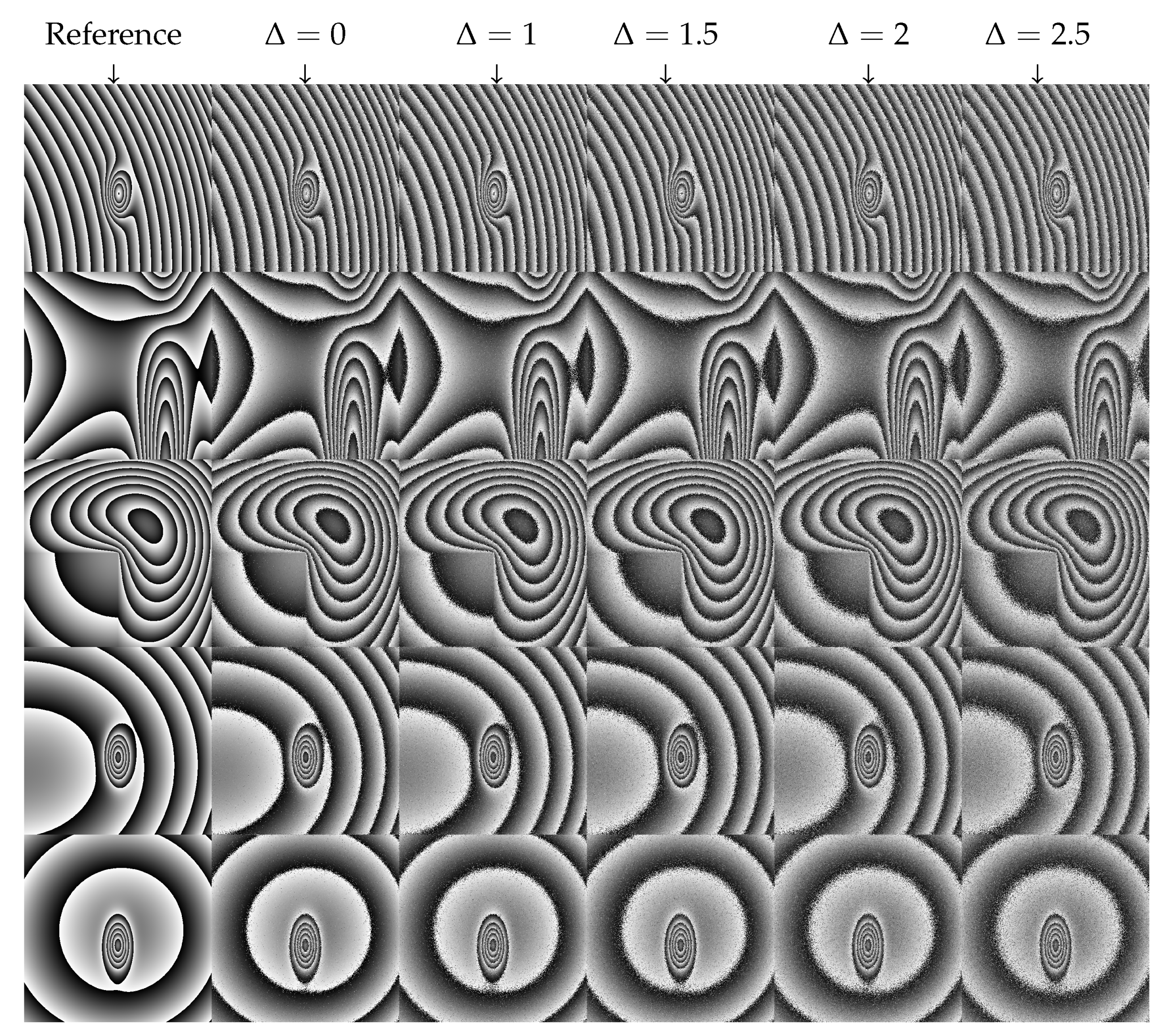
2.1. HOLODEEP Database

This database consists of five different types of noise-free phase fringe patterns and was used to train the models and for development purposes. Each pattern was degraded with realistic speckle decorrelation noise with statistics described in [23]. From each noise-free fringe pattern, five noisy fringe patterns controlled with a parameter, namely Δ , were generated with the simulator presented in [23], corresponding to different signal-to-noise-ratios (SNR) in the range [3 dB–12 dB]. The parameter Δ was used to mimic strongly degraded experimental phase data. The higher Δ , the smaller the SNR. In real conditions, there are several degradation sources that may induce more decorrelation noise than expected if all is perfect. As examples, the reconstruction of holographic data might not be perfectly in focus [30], the pixels could have a large active surface [3], the recording could have a low number of pixels or saturated pixels [31], the number of useful quantization bits could be insufficient [32], or there also could be wavelength changes between exposures [33]. As a consequence, all of these degradation sources have an increase in speckle decorrelation and then an increase in noise. Thus, using Δ is a useful way to obtain data with more noise in order to mimic possible experimental conditions. In the simulator described in [23], Δ corresponds to small changes in the wavelength between the two exposures. Therefore, adjusting Δ is useful to increase speckle decorrelation and thus to decrease the SNR in phase data. The simulated images, sized 1024 × 1024 pixels, were generated using Matlab and are available in the Matlab mat format or as tiff images. The 25 images used for training the models are shown in Figure 1.

2.2. DATAEVAL Database

This validation database consists of three images used for testing the model with images that have not been seen during the training or development processes. Two phase images, namely Test1 and Test2, were simulated using the simulator in Reference [23], similar to that for simulating the HOLODEEP database. The SNR of the two phases are respectively 3.05 dB (see Figure 2b) and 1.26 dB (see Figure 2e). These phase maps are not included in the HOLODEEP database. The last phase is an experimental noisy phase from vibration measured at 17 512 Hz, named Test3 with an SNR = 2.52 dB. The clean phase is shown in Figure 2g, the noisy phase is shown in Figure 2h, and the noisy phase obtained is shown in Figure 2i. The experimental setup and methodology to obtain such phase images is described in References [3,4]. The reader is invited to have a look at these papers for further details.

2.3. NATURAL Database

This database is generally used for natural gray-level image Gaussian de-noising. It consists of 400 images of size 180 × 180 . The RGB images are available at the link http://www.eecs.berkeley.edu/Research/Projects/CS/vision/grouping/BSR/BSR_bsds500.tgz (accessed on 2 June 2021). Noisy images were obtained by adding Gaussian noise with different SNR values (over 13 dB) directly to the clean images.

3. Baseline Approaches

The baseline results from the state-of-the-art are presented in Table 1. Phase error in radians was obtained from the HOLODEEP benchmark database and DATAEVAL images.

3.1. Signal Processing Approaches for Speckle De-Noising

Following the protocol described in [23], three algorithms from signal processing were tested: WFT2F, BM3D, and DtDWT. The results are given in terms of the standard deviation Δ ϕ of the phase error e i j defined in Equation (1), where N is the total number of pixels and e i j = ϕ d e n o i s e d ( i , j ) ϕ n o i s e f r e e ( i , j ) is the difference between the de-noised phase ϕ d e n o i s e d and the noise-free phase ϕ n o i s e f r e e at pixel ( i , j ) ,
Δ ϕ 2 = 1 N i , j e i j m e 2 ,
where m e is the average of e ( i , j ) over the set of pixels. Note that, since ϕ d e n o i s e d and ϕ n o i s e f r e e are calculated modulo 2 π , the difference e i j has to also be computed modulo 2 π according to e i j = arg [ exp ( i e i j ) ] .
The baseline results are given in terms of the average of Δ ϕ over the whole HOLODEEP database (i.e., 25 images sized 1024 × 1024 ) and with the three images of the DATAEVAL database. The results for the phase error Δ ϕ are summarized in Table 1.
The iteration number corresponds to how many times the noisy image has been processed by the de-noiser. From Table 1, one can be observed that only one iteration is required using WFT2F to obtain the best error at Δ ϕ = 0.026 rad with HOLODEEP because WTF2F uses a threshold on the decomposition 2D waveforms and the process ends after one iteration. Even with three iterations, the two other methods only reach Δ ϕ = 0.046 rad (DtDWT) and Δ ϕ = 0.068 rad (BM3D), thus confirming the best performance for WFT2F.

3.2. Deep Learning Approach for Speckle De-Noising

3.2.1. Data Augmentation

Since the training database might be not sufficiently extended, signal processing is used to increase it. For each original phase image, its cosine and sine versions ( × 2 ) are considered together with their transposed and phase shifted version ( π / 4 phase shift). This operation helps increase the number of original images by 8.

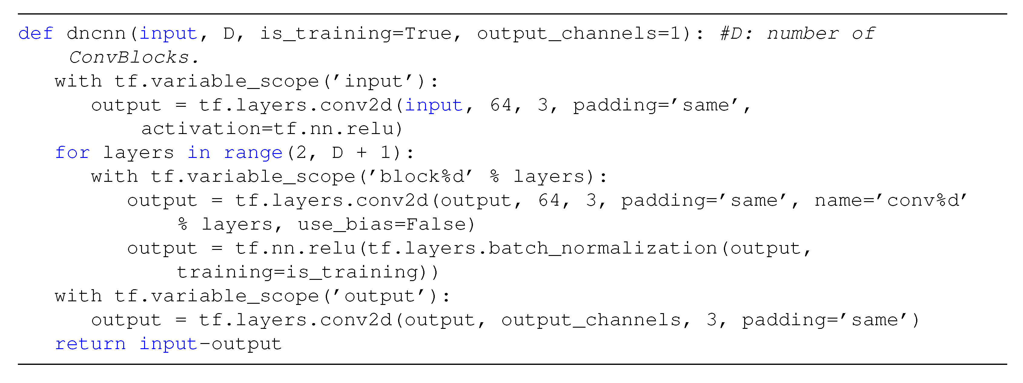
3.2.2. Baseline Implementation

The starting network considered in this section is the one proposed in [17], called DnCNN. It includes 59 layers organized upon a first input layer ( 3 × 3 convolutional layer and rectified linear units ReLU), 16 intermediate convolutional blocks (ConvBlocks: 3 × 3 × 64 convolutional layer, batch normalization and ReLU), and one output layer ( 3 × 3 × 64 convolutional layer), which is used to reconstruct the output noise. The de-noised image is the subtraction of the noisy image and the ouput noise. The loss function is an L2 loss between the reference and the predicted pixel values. The parameters of the training process are summarized in Table 2.
DnCNN network was pre-trained with 400 grey natural images sized 80 × 80 from the NATURAL database and optimized with the Adam algorithm. The blind Gaussian de-noiser was trained with a large set of noise levels, and a patch size of 50 × 50 . In the end, 128 × 3000 patches were cropped to train the model.
DL-3 [29] uses a pre-trained network https://www.mathworks.com/help/images/ref/dncnnlayers.html (accessed on 2 June 2021), which is then fine-tuned with data coming from the five fringe patterns, and a noise level fixed to two pixels per speckle grain in the simulator ( Δ = 0 ). The model was optimized using the stochastic gradient descent (SGD) algorithm. This situation corresponds to realistic digital online holographic recording conditions. Each phase image is then augmented eight times; thus, a total of 40 images sized 1024 × 1024 are used to adapt the model.

3.2.3. Baseline Results

The results obtained with DL-3 are reported in Table 1. The aforementioned deep learning model is compared to the signal processing approaches.
The results show that the DL-3 model slightly underperforms WFT2F on HOLODEEP with three iterations; however, the computation time is more interesting in the case of deep learning [34]. The addition of a noise estimator can further improve the performances. To be comparable with the baseline of de-noising algorithms, only one iteration is taken into account in the following experiments. From Table 1, with DL-3 and three iterations, the results are in the range of those from DtDWT and better than BM3D for phase maps Test1 and Test2 (speckle size at 4 pixels per grain). DL-3 was trained with only speckle grain at size 2, so this shows that the neural network can generalize with phase maps, which do not exactly correspond to the same trained speckle size.

4. Experimental Protocols

The global framework is presented in Figure 3, where the HOLODEEP database is used to train the networks. The evaluation metric is the phase error Δ ϕ computed between the predicted noise-free image and the noise-free reference (refer to Equation (1)).

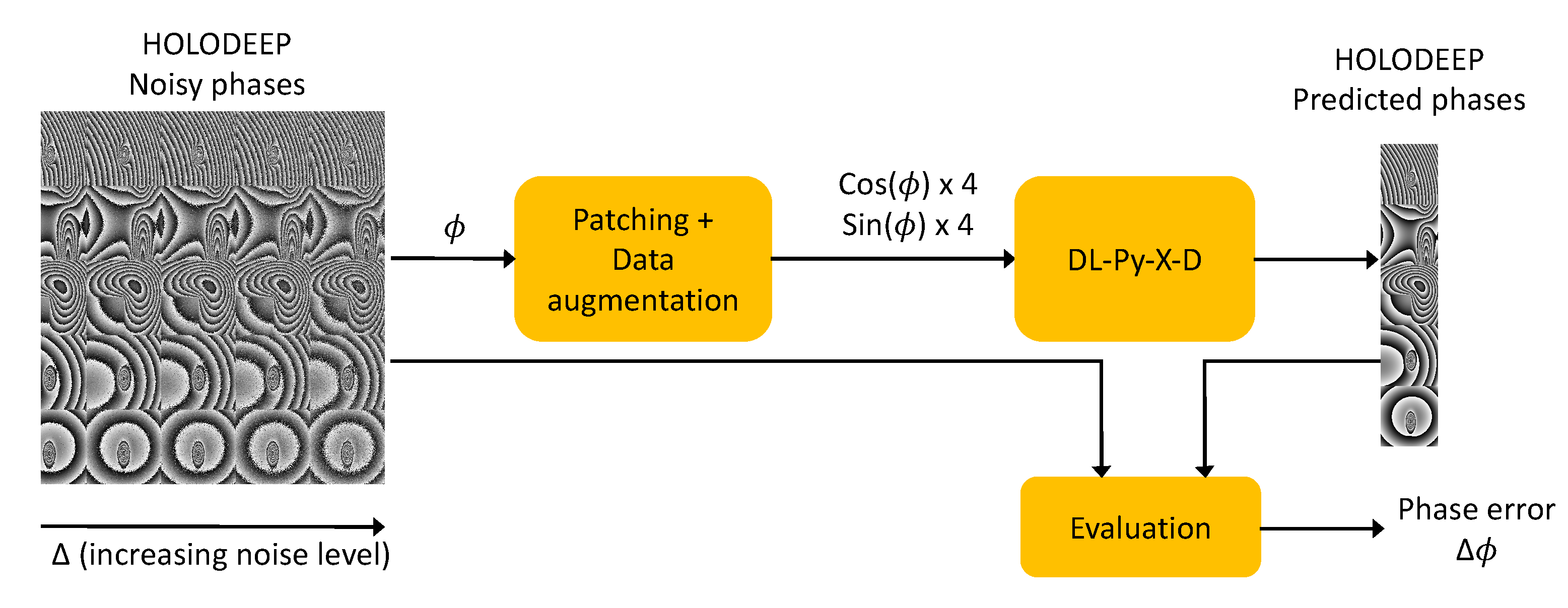
4.1. Data Pre-Processing and Implementation

The following experiments consider two independent parameters: the type of phase pattern (five patterns in the HOLODEEP database) and the level of speckle noise. For each original image sized 1024 × 1024 , candidate patches are extracted. These patches are sized 50 × 50 without any overlap. A random selection aims at extracting 384 patches per image. The seed is fixed once for all experiments in order to have reproducible patch selection. The whole patches are then shuffled in order to remove their dependency to a specific image. The cosine and sine input patches are normalized between 0 and 1.
A Tensorflow implementation was used as the starting point https://github.com/wbhu/DnCNN-tensorflow (accessed on 2 June 2021) and adapted with Matlab matrices as inputs https://git-lium.univ-lemans.fr/tahon/dncnn-tensorflow-holography/ (accessed on 2 June 2021). DL-Py is the Python implementation used in this paper. The architecture is described in Figure 4, where tf denotes the tensorflow library and D is the number of ConvBlocks. During the training step, the convergence is very fast in the first 10 epochs and then the loss function decreases continuously and slowly. The maximum number of epochs was fixed to 200 as the performances do not increase significantly with more epochs. However, due to cluster usage constraints, the training has to be stopped before the computing time overpasses a limit of 20 days. The number of epochs corresponding to the best phase error is included in Table 3. The final model is the one that reaches the best results with the development set. All models are trained on a cluster server with GPUs.

4.2. Evaluation Network Depth and Architecture

The network architecture slightly differs from the one proposed in the previous section. The model can be trained with different levels of noise (from Δ = 0 to 2.5), different noise-free phase fringe patterns (from 1 to 5), and different depths, i.e., different number of ConvBlocks ( D = 4 or 16). The following experiments intend to evaluate the influence of these factors on the de-noising performances of the deep learning models. The number of data and parameters used for training and evaluating the DL-Py networks are given in Table 2. The learning rate is set to L R = 0.001 , as it has been shown that this parameter has a large impact on the training duration and the results, with an Adam optimizer.
Depth of the network: Due to the high specificity of phase images, the goal is to ensure that the network does not overfit the training data. To do so, two different networks are trained, one with the original 16 ConvBlocks and the other with only 4 ConvBlocks. With the choice of four ConvBlocks as small model, training can be carried out rapidly while maintaining a certain level of complexity.
Noise level for training: Additionally, the network is supposed to be able to de-noise images that have a wide range of noise levels. Therefore, including various level of noise in the training data could help the network to do it. To do so, three networks are trained on different noise ranges.

4.3. Evaluation of a Pre-Trained Network

In a second step, how the network pre-trained on natural images with additional Gaussian noise can be better is estimated. Then, it is adapted to holographic phase images or to the direct use of a network trained entirely with holographic phase images.
Four hundred images of the NATURAL database are used to pre-train the network with the best architecture obtained in the previous section, i.e., four ConvBlocks (see Section 5). Once the network is pre-trained, a second fine-tuning stage is carried out using holographic images following the aforementioned protocol. The DL-nat-pt model corresponds to the model trained with natural images during 75 epochs, which seems reasonable regarding the 50 epochs used to train the original DnCNN [10]. Without fine-tuning, this model reaches Δ ϕ = 0.380 rad with the development set, which is not suitable at all for holographic images. The fine-tuning results are presented in the next section.

5. Results and Discussion

5.1. Network Depth and Architecture

The results obtained with HOLODEEP are summarized in Table 3. To help the reader, the model names the different parameters explicitly: DL-Py-X-D-z, with X being the maximum Δ in the training data, D being the depth of the model ( D = 4 or D = 16 ), and the optional z indicating if the model has been previously trained on natural images (pt).
When the training noise is Δ = 0 , the best results are obtained with a complex network (DL-Py-0-16, Δ ϕ = 0.057 rad). However, overall, the best results are obtained with only four ConvBlocks and a large range of training noise (DL-Py-2.5-4, Δ ϕ = 0.035 rad).
Introducing noise level diversity allows for drastically reducing the average phase error for all configurations. Especially the best configuration ( D = 4 ConvBlocks) lowers Δ ϕ from 0.058 rad ( Δ = 0 ) to 0.035 rad ( Δ = 0 2.5 ). This suggests that a reduced network trained with a large diversity is probably more generalizable than a deep network trained with very few data. One point remains uncertain: we are not sure whether the improvement observed on de-noising is due to the diversity of noise or to the larger amount of data used to train the network. The advantage of using a smaller number of layers is that the computation time is more than two times less.
An investigation of the results according to speckle noise level in the HOLODEEP images confirms that the higher the noise level, the higher the error in the restored phase map. Figure 5 details the values obtained during an evaluation on HOLODEEP according to their level of noise (parameter Δ ) with the three best models DL-Py-0-4 (train noise level Δ = 0 ), DL-Py-1.5-4 (train noise level Δ = 0 1.5 ), and DL-Py-2.5-4 (train noise level Δ = 0 2.5 ).
As aforementioned, DL-Py-2.5-4 is better on average than DL-Py-0-4 on HOLODEEP. However, the additional experiments show that this performance improvement is significantly more important on images with high noise level (−49% of relative reduction with Δ = 2.5 ) than with images with low noise (−31% with Δ = 0 ). These results underline the relevance of introducing a large diversity of patterns and noise levels during the training step if the application images to be processed also have high noise levels.

5.2. Pre-Training

Table 3 shows that the pre-trained model outperforms the initial models only when a small level of noise ( Δ = 0 ) is used for fine-tuning. This leads to the conclusion that pre-training the network on natural images helps to compensate for the lack of diversity in the specific training data and the relatively small amount of training data. Thse results confirm the advantage of using pre-trained models when the amount of specific target data is low [35].
Two hypotheses may explain the poor performances reached by the pre-trained model. The NATURAL and HOLODEEP databases differ on many points: additive Gaussian vs. multiplicative speckle noise and natural vs. wrapped phase images. Such a data difference could explain the poor performances obtained with pre-training: training a network with phase images using an initialization obtained on NATURAL database does not seem worthy in the present case. Therefore, training a network with phase data corrupted with speckle noise requires deeper investigated. The second hypothesis concerns the performance of the model trained on NATURAL data. Due to cluster usage constraints, the total number of epochs to train this model is 75 epochs. It aims to obtain a model performed on natural images. However, this number is higher than the 50 epochs used to train the original DnCNN model mentioned in [17] and the model might be too specific for natural images. As such models require a lot of resources to be trained, we did not have the opportunity to train it on a higher number of epochs. However, it is worth considering this aspect.

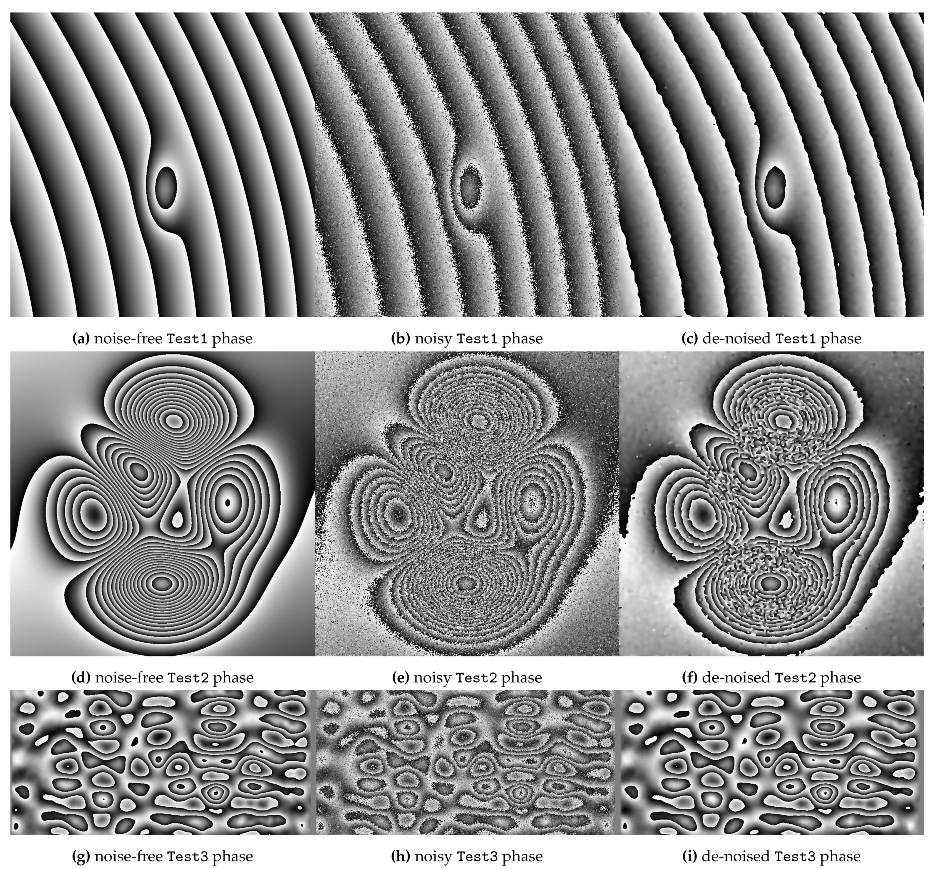
5.3. Evaluation on Target Images

Table 4 summarizes the performances obtained with the development and validation images. DL-Py-2.5-4 performs better on the training data HOLODEEP ( Δ ϕ = 0.035 rad) and on Test1 ( Δ ϕ = 0.072 rad). However, the performance is degraded when testing with Test2, which has a high level of noise, and with Test3, which is the phase image from vibration experiments. No clear answer can be given here. DL-Py-2.5-4 model is trained on a large number of data and noise; thus, it should be able to deal with a high level of noise. However, from the construction of the HOLODEEP database, there are a few redundancies in the phase images, and Test1 appears relatively similar to those in HOLODEEP while Test2 and Test3 are not. Therefore, the model might not be easily generalizeable to unseen images. Another hypothesis is that the structure of the model implies additive noise, which could be relevant for a small SNR but not for a high SNR where speckle noise is clearly multiplicative. The model that best generalized on test2 and Test3 is the one trained on a medium range of speckle noise (DL-Py-1.5-4). This model is even able to outperform the baseline WFT2F on the experimental vibration map Test3 phase image. Figure 2 shows how these images from DATAEVAL are de-noised by the best model. Therefore, the proposed networks are able to reach interesting performances in comparison to WFT2F, especially for some specific experimental images. These networks have the advantage of being faster to train than the DL-3 network as they only contains four ConvBlocks.
Regarding pre-trained models, it seems that they are not generalizable on unseen images except DL-Py-0-4-pt, which obtains Δ ϕ = 0.105 rad with Test3. Additional experiments show that models trained with more epochs can improve the performances on Test1 but degrade on Test2 and Test3.

6. Conclusions

This paper discusses holographic phase images de-noising and presents an alternative approach that is specific for speckle noise. The results show that a pre-trained model is not useful except when the amount and diversity of simulated data are low. In this case, the pre-training compensates for the lack of data. The experiments also demonstrate that the use of very deep networks is not necessary and that the use of four ConvBlocks yields reliable performances in comparison to WFT2F. Reduced networks also have the advantage of being faster to train. This study also addresses the issue of the generalization of the networks. It appears that WFT2F remains the best algorithm for phase images with a high level of noise (Test2). However, the best model is able to outperform the baseline of WFT2F with experimental data (Test3). The poor performance of DL-Py models with phase images with a high level of noise may be related to the additive hypothesis implemented in the network itself. A multiplicative model will be investigated in the future. Further work intends to improve speckle de-noising by combining the advantages of the two approaches following preliminary works on the addition of a noise estimator [34]. Other data augmentation functions will be implemented in order to increase the amount of training data. In addition, the construction of a new database with an increased diversity of fringe images would be of interest to train the networks with a high diversity of patterns.

Author Contributions

M.T. prepared the neural networks, S.M. and P.P. prepared the database and evaluation process. M.T., S.M. and P.P. analyzed the experimental results. All authors have read and agreed to the published version of the manuscript.

Funding

The research work has no external funding.

Institutional Review Board Statement

Not applicable.

Informed Consent Statement

Not applicable.

Data Availability Statement

HOLODEEP database is freely available [DOI:10.13140/RG.2.2.20819.78885].

Acknowledgments

We thank LIUM for authorization access to the GPU cluster.

Conflicts of Interest

The authors declare no conflict of interest.

References

  1. Picart, P.; Li, J. Digital Holography; John Wiley & Sons, Ltd.: London, UK, 2012. [Google Scholar]
  2. Ghiglia, D.C.; Pritt, M.D. Two-Dimensional Phase Unwrapping: Theory, Algorithms, and Software; Wiley: New York, NY, USA, 1998. [Google Scholar]
  3. Poittevin, J.; Gautier, F.; Pézerat, C.; Picart, P. High-speed holographic metrology: Principle, limitations, and application to vibroacoustics of structures. Opt. Eng. 2016, 55, 121717–121729. [Google Scholar] [CrossRef]
  4. Lagny, L.; Secail-Geraud, M.; Le Meur, J.; Montresor, S.; Heggarty, K.; Pezerat, C.; Picart, P. Visualization of travelling waves propagating in a plate equipped with 2D ABH using wide-field holographic vibrometry. J. Sound Vib. 2019, 461, 114925. [Google Scholar] [CrossRef]
  5. Meteyer, E.; Montresor, S.; Foucart, F.; Le Meur, J.; Heggarty, K.; Pezerat, C.; Picart, P. Lock-in vibration retrieval based on high-speed full-field coherent imaging. Sci. Rep. 2021, 11, 1–15. [Google Scholar] [CrossRef]
  6. Dabov, K.; Foi, A.; Katkovnik, V.; Egiazarian, K. Image denoising with block-matching and 3D filtering. In Proceedings of the SPIE, Image Processing: Algorithms and Systems, Neural Networks, and Machine Learning, San Jose, CA, USA, 16–18 January 2006; Volume 6064, p. 606414. [Google Scholar]
  7. Selesnick, I.W.; Baraniuk, R.G.; Kingsbury, N.C. The dual-tree complex wavelet transform. IEEE Signal Process. Mag. 2005, 22, 123–151. [Google Scholar] [CrossRef] [Green Version]
  8. Kemao, Q.; Wang, H.; Gao, W. Windowed Fourier transform for fringe pattern analysis: Theoretical analyses. Appl. Opt. 2008, 47, 5408–5419. [Google Scholar] [CrossRef]
  9. Jain, V.; Seung, S. Natural image denoising with convolutional networks. In Advances in Neural Information Processing Systems; Koller, D., Schuurmans, D., Bengio, Y., Bottou, L., Eds.; Curran Associates, Inc.: Red Hook, NY, USA, 2009; Volume 21, pp. 769–776. Available online: https://www.researchgate.net/publication/221620211_Natural_Image_Denoising_with_Convolutional_Networks (accessed on 2 June 2021).
  10. Zeng, T.; So, H.K.H.; Lam, E.Y. Computational image speckle suppression using block matching and machine learning. Appl. Opt. 2019, 58, B39–B45. [Google Scholar] [CrossRef]
  11. Krishnan, J.P.; Bioucas-Dias, J.M.; Katkovnik, V. Dictionary learning phase retrieval from noisy diffraction patterns. Sensors 2018, 18, 4006. [Google Scholar] [CrossRef] [Green Version]
  12. He, K.; Zhang, X.; Ren, S.; Sun, J. Deep residual learning for image recognition. In Proceedings of the 2016 IEEE Conference on Computer Vision and Pattern Recognition (CVPR), Las Vegas, NV, USA, 27–30 June 2016; pp. 770–778. [Google Scholar]
  13. Goodfellow, I.J.; Pouget-Abadie, J.; Mirza, M.; Xu, B.; Warde-Farley, D.; Ozair, S.; Courville, A.; Bengio, Y. Generative adversarial nets. In Proceedings of the 27th International Conference on Neural Information Processing Systems (NIPS)-Volume 2, Montreal, QC, Canada, 8–13 December 2014; MIT Press: Cambridge, MA, USA, 2014; pp. 2672–2680. [Google Scholar]
  14. Barbastathis, G.; Ozcan, A.; Situ, G. On the use of deep learning for computational imaging. Optica 2019, 6, 921–943. [Google Scholar] [CrossRef]
  15. Rivenson, Y.; Zhang, Y.; Günaydın, H.; Teng, D.; Ozcan, A. Phase recovery and holographic image reconstruction using deep learning in neural networks. Light Sci. Appl. 2018, 23, 17141. [Google Scholar] [CrossRef] [PubMed]
  16. Wang, F.; Wang, H.; Li, G.; Situ, G. Learning from simulation: An end-to-end deep-learning approach for computational ghost imaging. Opt. Express 2019, 27, 25560–25572. [Google Scholar] [CrossRef]
  17. Zhang, K.; Zuo, W.; Chen, Y.; Meng, D.; Zhang, L. Beyond a Gaussian denoiser: Residual learning of Deep CNN for image denoising. IEEE Trans. Image Process. 2017, 26, 3142–3155. [Google Scholar] [CrossRef] [Green Version]
  18. Shi, W.; Jiang, F.; Zhang, S.; Wang, R.; Zhao, D.; Zhou, H. Hierarchical residual learning for image denoising. Signal Process. Image Commun. 2019, 76, 243–251. [Google Scholar] [CrossRef]
  19. Choi, G.; Ryu, D.; Jo, Y.; Kim, Y.S.; Park, W.; Min, H.S.; Park, Y. Cycle-consistent deep learning approach to coherent noise reduction in optical diffraction tomography. Opt. Express 2019, 27, 4927–4943. [Google Scholar] [CrossRef] [PubMed] [Green Version]
  20. Yuan, Q.; Zhang, Q.; Li, J.; Shen, H.; Zhang, L. Hyperspectral image denoising employing a spatial spectral deep residual convolutional neural network. IEEE Trans. Geosci. Remote Sens. 2019, 57, 1205–1218. [Google Scholar] [CrossRef] [Green Version]
  21. Jeon, W.; Jeong, W.; Son, K.; Yang, H. Speckle noise reduction for digital holographic images using multi-scale convolutional neural networks. Opt. Lett. 2018, 43, 4240–4243. [Google Scholar] [CrossRef] [PubMed]
  22. Ma, Y.; Chen, X.; Zhu, W.; Cheng, X.; Xiang, D.; Shi, F. Speckle noise reduction in optical coherence tomography images based on edge-sensitive cGAN. Biomed. Opt. Express 2018, 9, 5129–5146. [Google Scholar] [CrossRef] [PubMed]
  23. Montrésor, S.; Picart, P. Quantitative appraisal for noise reduction in digital holographic phase imaging. Opt. Express 2016, 24, 14322–14343. [Google Scholar] [CrossRef]
  24. Montrésor, S.; Picart, P.; Sakharuk, O.; Muravsky, L. Error analysis for noise reduction in 3D deformation measurement with digital color holography. J. Opt. Soc. Am. B 2017, 34, B9–B15. [Google Scholar] [CrossRef]
  25. Perez, L.; Wang, J. The effectiveness of data augmentation in image classification using deep learning. arXiv 2017, arXiv:1712.04621. [Google Scholar]
  26. Simonyan, K.; Zisserman, A. Very deep convolutional networks for large-scale image recognition. In Proceedings of the 3rd International Conference on Learning Representations, ICLR 2015, San Diego, CA, USA, 7–9 May 2015; pp. 1–14. [Google Scholar]
  27. Han, Z.; Yu, S.; Lin, S.B.; Zhou, D.X. Depth selection for deep ReLU nets in feature extraction and generalization. IEEE Trans. Pattern Anal. Mach. Intell. 2020. [Google Scholar] [CrossRef]
  28. Goodfellow, I.; Bengio, Y.; Courville, A. Deep Learning; MIT Press: Cambridge, MA, USA, 2016. [Google Scholar]
  29. Montresor, S.; Tahon, M.; Laurent, A.; Picart, P. Computational de-noising based on deep learning for phase data in digital holographic interferometry. APL Photonics 2020, 5, 030802. [Google Scholar] [CrossRef] [Green Version]
  30. Picart, P.; Montresor, S.; Sakharuk, O.; Muravsky, L. Refocus criterion based on maximization of the coherence factor in digital three-wavelength holographic interferometry. Opt. Lett. 2017, 42, 275–278. [Google Scholar] [CrossRef] [PubMed]
  31. Picart, P.; Tankam, P.; Song, Q. Experimental and theoretical investigation of the pixel saturation effect in digital holography. J. Opt. Soc. Am. A 2011, 28, 1262–1275. [Google Scholar] [CrossRef] [PubMed]
  32. Poittevin, J.; Picart, P.; Gautier, F.; Pezerat, C. Quality assessment of combined quantization-shot-noise-induced decorrelation noise in high-speed digital holographic metrology. Opt. Express 2015, 23, 30917–30932. [Google Scholar] [CrossRef]
  33. Baumbach, T.; Kolenovic, E.; Kebbel, V.; Jüptner, W. Improvement of accuracy in digital holography by use of multiple holograms. Appl. Opt. 2006, 45, 6077–6085. [Google Scholar] [CrossRef]
  34. Montresor, S.; Tahon, M.; Laurent, A.; Picart, P. An iterative scheme based on deep learning combined with input noise estimator for phase data processing in digital holographic interferometry. In Proceedings of the Imaging and Applied Optics Congress, Washington, DC, USA, 22–26 June 2020; p. HTu4B.4. [Google Scholar]
  35. Macary, M.; Tahon, M.; Estève, Y.; Rousseau, A. On the use of self-supervised pre-trained acoustic and linguistic features for continuous speech emotion recognition. In Proceedings of the 2021 IEEE Spoken Language Technology Workshop (SLT), IEEE, Shenzhen, China, 19–22 January 2021; pp. 373–380. [Google Scholar]
Figure 1. HOLODEEP training phase images: five patterns (in lines) with simulated speckle noise with five values of Δ (in columns).
Photonics 08 00255 g001
Figure 2. Noise-free (left), noisy (middle), and de-noised (right) phase images from DATAEVAL. De-noising was performed using the DL-Py-1.5-4 model.
Photonics 08 00255 g002
Figure 3. Global overview of the training stage of the system.
Photonics 08 00255 g003
Figure 4. Python code with tensorflow framework (as tf), which defines the model architecture.
Photonics 08 00255 g004
Figure 5. Δ ϕ (rad) obtained on HOLODEEP with best model ( D = 4 ). Δ -AVG indicates the error averaged on the 25 images, Δ = X indicates the error averaged on the noisy images obtained with Δ = X .
Photonics 08 00255 g005
Table 1. Baseline standard deviation of the phase errors ( Δ ϕ in rad) obtained on the 25 images from the HOLODEEP database (in average) and individual images from DATAEVAL. Iter is the number of times that the image passes through the de-noiser.
Method# iterHOLODEEPDATAEVAL
25 ImagesTest1Test2Test3
WFT2F10.0260.0440.1640.105
DtDWT1–30.0460.0780.5190.214
BM3D1–30.0680.1130.5800.094
ine DL-310.0410.1070.5850.105
DL-330.0310.0780.5590.077
Table 2. Parameters used to train the networks. Δ lies for the simulated speckle noise.
DnCNN [17]DL-3 [29]DL-Py
original size 180 × 180 1024 × 1024 1024 × 1024
patch size 50 × 50 50 × 50 50 × 50
batch size128128128
learning rate0.1 to 0.0010.00060.001; 0.0005
# epochs501920<200
noise typeGaussianGauss+specklespeckle
noise σ [ 0 ; 55 ] , μ = 0 Δ = 0 Δ = 0 Δ = 0 1.5 Δ = 0 2.5
SNR (dB) range>137.32 − 11.467.32 − 11.465.08 − 11.463.10 − 11.46
# train images400 5 × 8 = 40 5 × 8 = 40 5 × 3 × 8 = 120 5 × 5 × 8 = 200
# patches 128 × 3000 = 384 k 384 × 40 = 15.3 k 384 × 40 = 15.3 k 384 × 120 = 46.1 k 384 × 200 = 76.8 k
Table 3. Phase errors ( Δ ϕ in rad), obtained with one iteration on HOLODEEP. The best configurations are presented in bold font. Three training sets are used, each corresponding to a larger diversity of noise, and the number of patches used to train the model in each case is given. The model names are given for each configuration. The best epoch is given relative to the total number of epochs used to train the model.
Trained on HOLODEEPPre-Trained
Δ (#patch)D1644
0 (15.3k)modelDL-Py-0-16DL-Py-0-4DL-Py-0-4-pt
BestEpoch/Max195/200200/200190/200
Δ ϕ 0.0570.0580.055
ine 0–1.5 (46.1k)modelDL-Py-1.5-16DL-Py-1.5-4DL-Py-1.5-4-pt
BestEpoch/Max70/70140/15085/95
Δ ϕ 0.0420.0400.045
ine 0–2.5 (76.8k)modelDL-Py-2.5-16DL-Py-2.5-4DL-Py-2.5-4-pt
BestEpoch/Max40/5090/9550/55
Δ ϕ 0.0380.0350.048
Table 4. Δ ϕ (rad) obtained on the HOLODEEP database (in average) and individual images from DATAEVAL with one iteration. The best epochs for the pre-trained and trained models on the HOLODEEP validation database.
MethodHOLODEEPDATAEVAL
25 ImagesTest1Test2Test3
WFT2F0.0260.0440.1630.105
DL-30.0410.1070.5850.105
DL-Py-0-40.0580.1420.6290.117
DL-Py-0-4-pt0.0550.1460.6290.105
DL-Py-1.5-40.0400.0950.5930.103
DL-Py-1.5-4-pt0.0450.1120.6090.111
DL-Py-2.5-40.0350.0720.5970.109
DL-Py-2.5-4-pt0.0480.0970.6600.134
Publisher’s Note: MDPI stays neutral with regard to jurisdictional claims in published maps and institutional affiliations.

