Article

Adaptation of the Standard Off-Axis Digital Holographic Microscope to Achieve Variable Magnification

1
Shanghai Institute of Optics and Fine Mechanics, Chinese Academy of Sciences, Shanghai 201800, China
2
School of Electrical and Electronic Engineering, University College Dublin, Dublin 4 Belfield, Ireland
3
Department of Electronic Engineering, Maynooth University, W23 Maynooth, Ireland
4
Institute of Micromechanics and Photonics, Warsaw University of Technology, 8 Sw. Andrzeja Boboli Street, 02-525 Warsaw, Poland
5
Department of Computer Science, Maynooth University, W23 Maynooth, Ireland
*
Author to whom correspondence should be addressed.
Photonics 2021, 8(7), 264; https://doi.org/10.3390/photonics8070264
Submission received: 24 May 2021 / Revised: 24 June 2021 / Accepted: 2 July 2021 / Published: 7 July 2021
(This article belongs to the Special Issue Holography)

Abstract

:
Traditional microscopy provides only for a small set of magnifications using a finite set of microscope objectives. Here, a novel architecture is proposed for quantitative phase microscopy that requires only a simple adaptation of the traditional off-axis digital holographic microscope. The architecture has the key advantage of continuously variable magnification, resolution, and Field-of-View, by simply moving the sample. The method is based on combining the principles of traditional off-axis digital holographic microscopy and Gabor microscopy, which uses a diverging spherical wavefield for magnification. We present a proof-of-concept implementation and ray-tracing is used to model the magnification, Numerical Aperture, and Field-of-View as a function of sample position. Experimental results are presented using a micro-lens array and shortcomings of the method are highlighted for future work; in particular, the problem of aberration is highlighted, which results from imaging far from the focal plane of the infinity corrected microscope objective.

1. Introduction

Holography [1,2] is an imaging methodology that involves separate processes for recording and replay in order to recover the image. For several decades, photographic films were required to record the holograms and the reconstruction process was also implemented optically; however, in the past two decades this approach has been superseded by the application of a digital area sensor to record the holograms, and the reconstruction process is performed using a set of computer algorithms that simulate optical replay [3,4]. Several architectures exist for optically recording a digital hologram. The off-axis technique, initially developed for the case of photographic film [2], enables separation of the noisy DC and twin terms that are inherent in holography. This approach was first used with digital sensors by Cuche et al. [5] whereby image reconstruction is numerical in nature and spatial filtering is achieved in the discrete Fourier transform domain to isolate the real image. Refocusing can also be achieved using numerical propagation algorithms [5,6,7,8].
Digital holographic microscopy [5,6] (DHM) is an extension of digital holography, whereby a coherently illuminated object wavefield is first magnified using a microscope objective before recording using digital holography. DHM enables the quantitative phase image of a microscopic sample to be recorded and has been shown to be a powerful technique for the analysis of biological cells [9,10]. Building on the work of Leith and Upatieks [2] in the area of material holography, arguably the most common architecture for implementing DHM is to use an off-axis reference beam [5], which results in the separation of the twin images in the discrete Fourier domain of the recorded digital image.
Digital in-line holographic microscopy [7,11,12,13,14,15] (DIHM) is a related technique using a much simpler architecture and is based on Gabor’s original setup [1]. In DIHM, a pinhole generates a diverging spherical wave, which is incident on a sample some small distance away. The resultant diffraction pattern is captured by a digital sensor and an image can be reconstructed numerically using a variety of different algorithms [7,11,16]. This approach has the advantage of continuously variable magnification/Field-of-View by moving the sample between the pinhole and the sensor, with low magnifications (when the sample is placed atop the sensor) still providing high resolution [17,18,19]. However, the reconstructed image is marred by the presence of the DC term and the twin image, which complicates retrieval of the phase image; furthermore, the method is applicable only to weakly scattering objects [15,20]. These problems can be overcome using a multi height approach [17,18,21,22] or more recently using deep learning in neural networks [19] to recover the phase image. However, such approaches are not easily applicable to dynamically changing scenes.
The objective of this letter is to present a proof-of-concept combination of the standard off-axis DHM and DIHM architectures. The proposed setup, described in Section 2, has the key advantage of DIHM relating to continuously variable magnification/Field-of-View by simply moving the sample, but overcomes the disadvantages listed above. It is shown that this can be achieved by a simple adaptation of a typical off-axis DHM system, which involves only the addition of a Fourier transforming lens before the sensor, as well as the adjustment of the condenser lens to provide diverging illumination; this latter idea is borrowed directly from the DIHM modality. In the sections that follow, the concepts of the A B C D ray-transfer matrix and ray-tracing are used to design a reconstruction algorithm and to estimate the Numerical Aperture and Field-of-View of the system for each object position.

2. Optical System

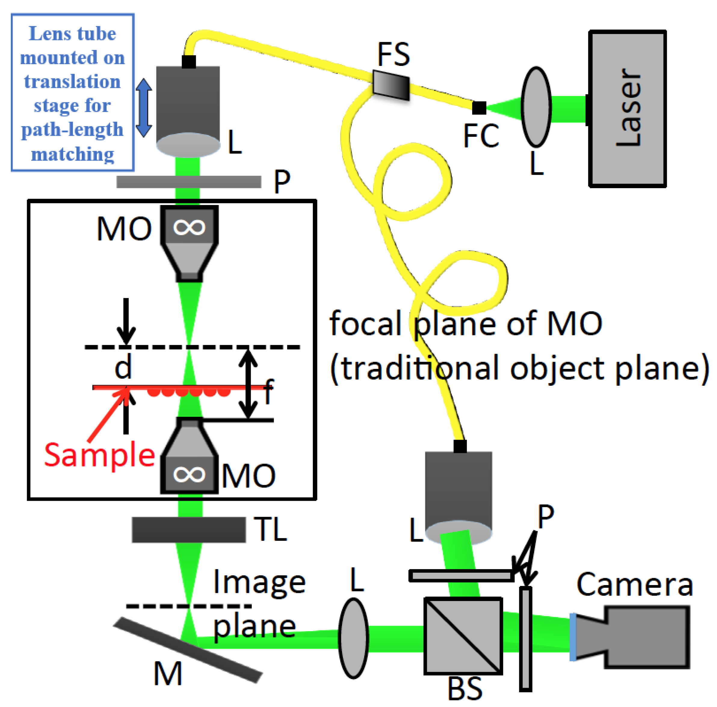
2.1. Experimental Setup

In Figure 1 the proposed optical setup is illustrated, which is based on a small adaptation of a traditional off-axis DHM setup that was previously described in ref. [23]. A laser diode source (CNI Laser MGL-III-532) operating at a power of 10 mW and with wavelength 532 nm is coupled into a single mode optical fiber (Thorlabs; FC532-50B-FC) that splits into two output fibers with a 50 / 50 power ratio. The first fiber output is collimated by a plano convex lens with focal length 5 cm and passed through a linear polariser (Thorlabs; LPVISE100-A) and a condenser lens (Olympus; UMplanFl 50 × / 0.8 ) to illuminate the sample. The fiber output and collimating lens are both fixed within a single lens tube, which is mounted on a translation stage (Thorlabs; CT1) and facilitates path length matching.
The condenser focuses a collimated beam to a diffraction limited spot at the focal plane of the MO, (Leitz; 32 × / 0.6 ) which has a Numerical Aperture of 0.6 and a working distance of 3.5 mm. Both the condenser and the MO are infinity corrected objectives, and are spatially separated by the sum of their working distances. The focused spot is, therefore, located in the focal plane of both objectives. The sample is positioned at some plane a distance d from this focused spot and is, therefore, illuminated by a diverging wavefield, similar to the case of DIHM. The sample is mounted on an electronic translation stage (ASI; MS-2000, LS-50, LX-4000). The wavefield that is scattered by the object passes through the MO, followed by a tube lens with focal length 200 mm (Thorlabs; TTL200) and a convex lens also with 200 mm focal length (Thorlabs; LB1945-A), which is positioned 200 mm from the (traditional) image plane at the back of the tube lens and 200 mm from the sensor plane; this latter lens performs an optical Fourier transformation between the image plane of the microscope and the sensor. A polarising cube beam splitter (Thorlabs; PBS252) combines the object wavefield with a reference wavefield, which is produced from the output of the second fiber, which is collimated by a lens and directed at the camera at a small angle. A second linear polariser (Thorlabs; LPVISE100-A) is positioned before the CMOS sensor (Basler; acA200-340 km), which has 2048 × 1088 pixels of size 5.5 μ m. The coherence length of the laser is 0.1 mm, which ensures that noise from back reflections is reduced; however, this requires that the path lengths are suitably matched, which is achieved using different fiber lengths for both paths. The final linear polariser ensures high hologram diffraction efficiency. All optical elements were obtained from Thorlabs with anti-reflection coating for the visible region. The angle of reference with respect to the camera normal, is selected to ensure separation of the twin images from the other terms in the spatial frequency domain [20]; this enables isolation of the real image by filtering using the discrete Fourier transform (DFT) [5]. This is possible if the support of the object wavefield in the spatial frequency domain is sufficiently limited and the frequency shift imparted by the angle of the reference is sufficiently large; for more details see Chapters 6 and 9 of Goodman [20]. In Section 3, image formation for this system is investigated based on diffraction theory, and it shown that the mapping between the object plane and the camera plane can be modeled by a simple Fresnel transform as well as a variable magnification that is equivalent to that provided by DIHM.

2.2. Comparison with Setup for Traditional Off-Axis Digital Holographic Microscopy

The optical system described above is based on an adaptation of the traditional off-axis DHM architecture, which is commercially employed by LynceeTec and others. The key features of this adaptation are as follows:
  • The distance between the condenser lens and the MO is altered to ensure that they are physically separated by a distance equal to the sum of their working distances. Since both objectives are infinity corrected objectives, this ensures that the focal planes of both objectives are coplanar. Furthermore, it ensures that a collimated laser beam that enters the back aperture of the condenser will result in a collimated laser beam exiting the back aperture of the MO.
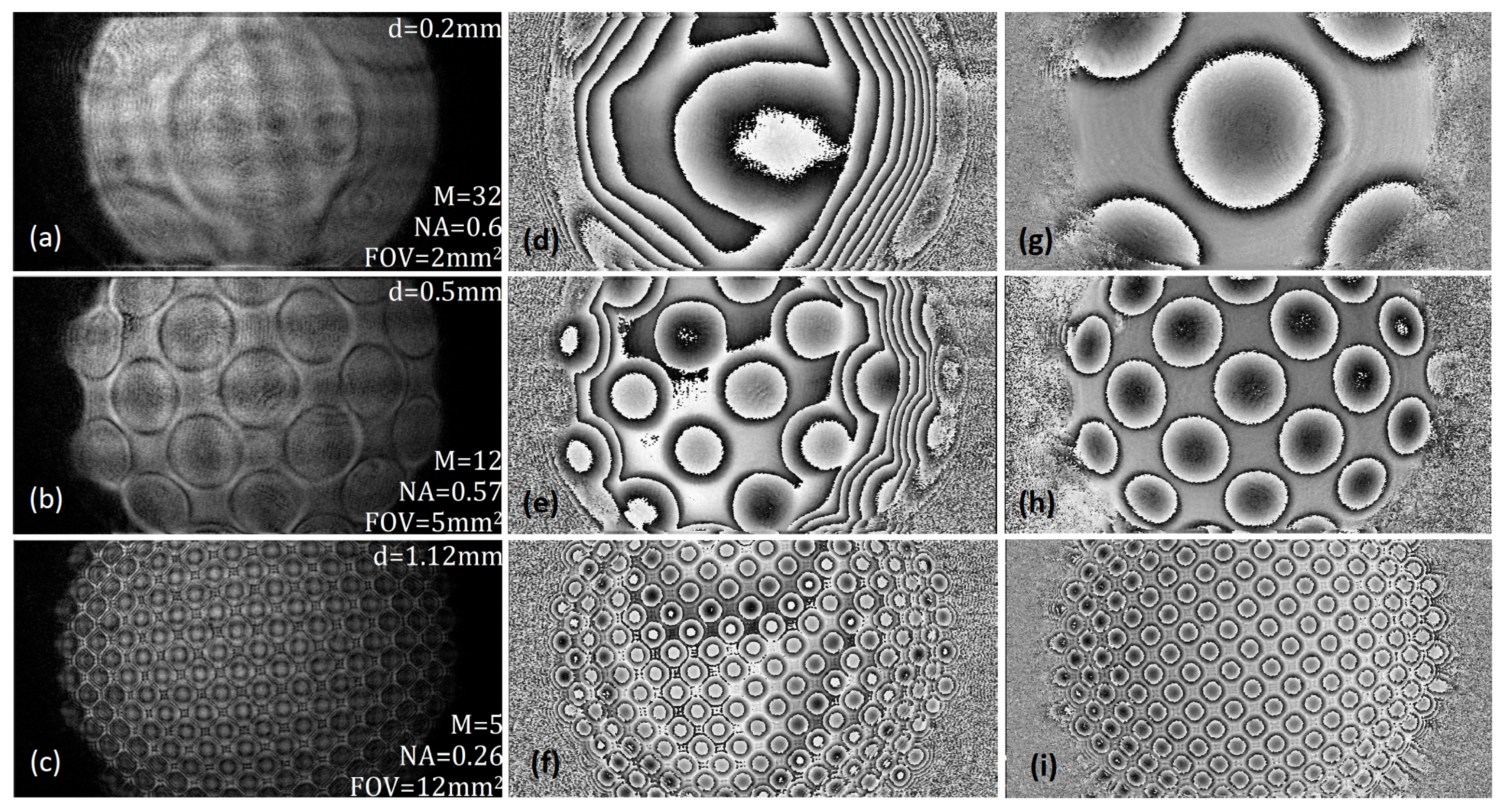
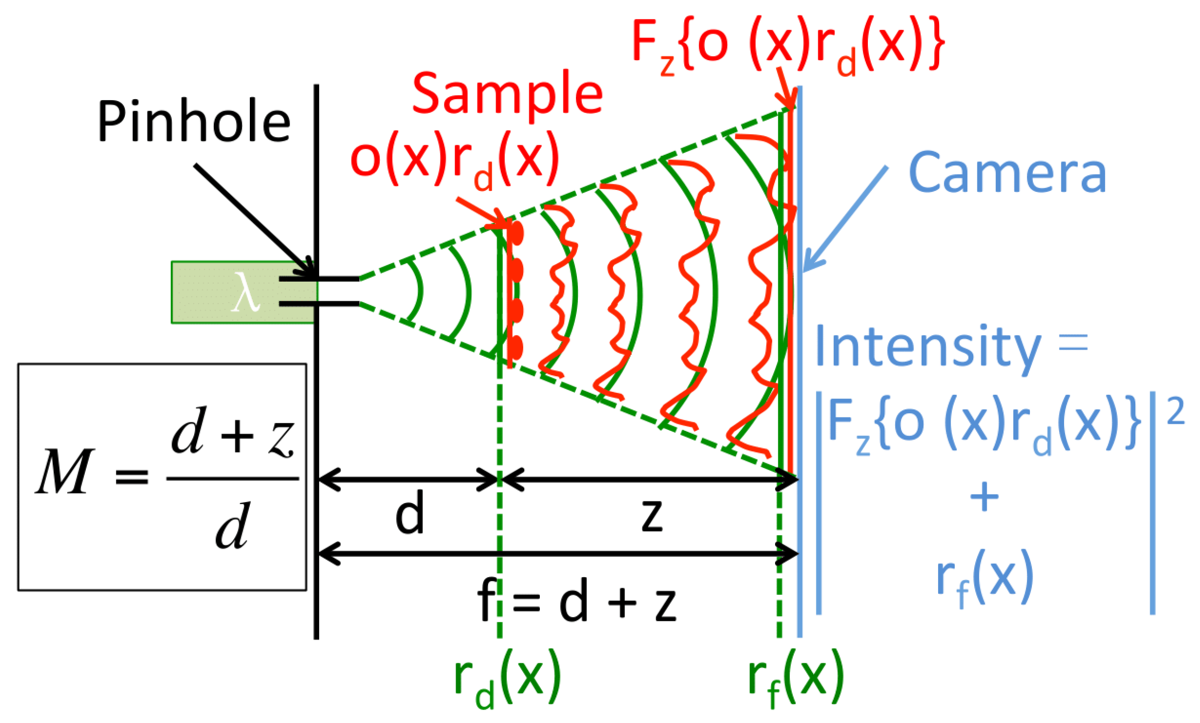
  • The sample is no longer limited to a single position at the focal plane of the MO as for the case of traditional off-axis DHM. Instead, the sample can occupy any plane between the focal plane of the MO and the surface of the MO. The location of the sample in this range will determine the magnification of the imaging system with a maximum value of infinity, when the sample is located at the focal plane, and a minimum value that must be less than unity, when the sample is located at the surface of the MO. The relationship between sample location and magnification is explored in more detail in Section 5.
  • The camera is not positioned in the traditional image plane of the microscope (i.e., at the focal plane of the tube lens). Instead, a Fourier transforming lens is inserted between the image plane and the camera plane. Thus, a collimated laser beam entering the condenser aperture, and exiting the back aperture of the MO, will be imaged onto the camera. This step guarantees that the full Field-of-View that is afforded by any given (variable) magnification can be captured by the system. This step also ensures that there will be a simple relationship between the object plane and camera plane for any arbitrary object location and resultant magnification, which is described in more detail in Section 4.

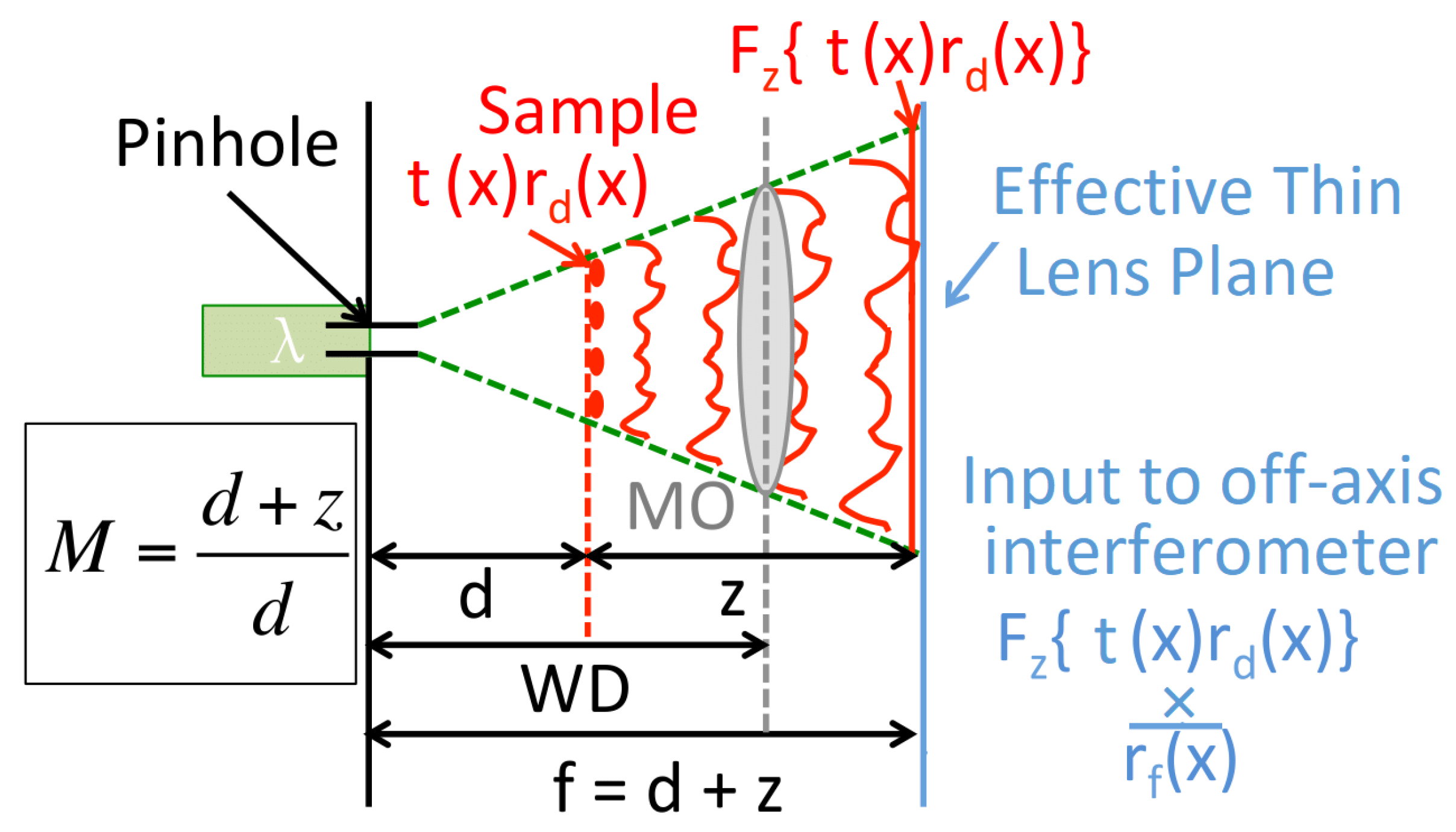
3. Extending the Principles of DIHM to Off-Axis DHM with a Microscope Objective

In this section, a model is presented that relates the object’s transmission function to the complex wavefield that is captured by the camera in Figure 1. This model facilitates the design of a numerical reconstruction algorithm in Section 4 as well as the derivation of the Magnification, Numerical Aperture, and Field-of-View of the microscope in Section 5, all of which vary continuously as a function of object position. Central to this model are the concepts of ray optics and diffraction theory, which are reviewed in Appendix A. The model presented here builds directly on the established model for DIHM, which is reviewed in detail in Appendix B.
An abstraction of the physical system described in the previous section is illustrated in Figure 2; a comparison of this figure with the equivalent figure for DIHM in Figure A1 reveals several features that are common to both. For both setups, a spherical beam emerges from a pinhole with a wavelength λ ; practically, this is generated using a beam focused by an MO as illustrated in Figure 1. Following propagation of a distance d, this diverging spherical field is incident upon an object, with transmittance t ( x ) , which is identical to the DIHM case shown in Figure A1. For the system proposed here, however, we do not need to make any assumption about the weakly scattering object as defined in Equation (A6), since we do not need to rely upon the unscattered wavefield r f ( x ) to generate an in-line interference pattern.
In the case of DIHM, an intensity pattern is recorded by a camera a further distance z away from the object plane, and this intensity pattern is assumed to contain an interference pattern between the wavefield scattered by the weak object and the unscattered field. For the system proposed here, a microscope objective (MO) replaces the camera, which we model as a thin lens in the same plane as the camera. In this way, we will demonstrate in the proceeding sections that it is an identical form of variable magnification can be obtained for the off-axis system as for the case of DIHM.
By positioning the MO (with focal length f) such that f = d + z , its effect can be approximated as a chirp function that is the conjugate of the unscattered wavefield in the interference pattern in DIHM, i.e., the field immediately after the thin-lens approximation can be described as t ( x ) r f * ( x ) , which is identical to the real image term in the DIHM hologram. The lens effectively collimates the diverging wavefield that has been scattered by the object, approximately limiting it to a light-tube [24] no matter the position of the object in the range of possible values of d. An off-axis interferometer is used to record this term in isolation, which can provide for a reconstruction of the quantitative phase image of t ( x / M ) as demonstrated in the following sections, in which the numerical reconstruction algorithm is derived and it shown that the overall opto-numerical system has a magnification M that is identical to the magnification term in DIHM.

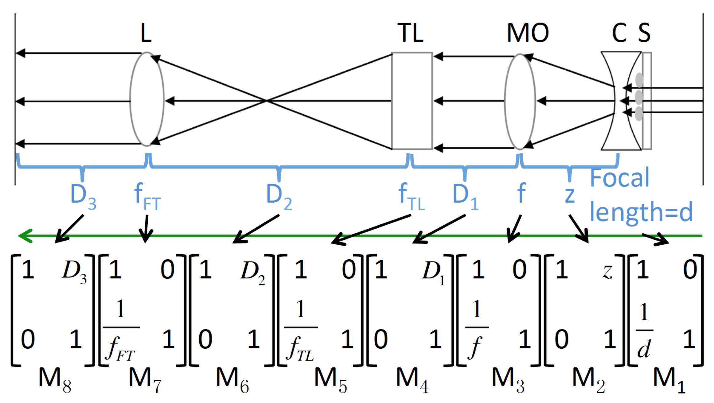
4. Numerical Reconstruction

The overall system that maps in the object plane to the sensor plane is illustrated in Figure 3. Contrary to convention, light is illustrated to propagate from the input (sample) plane on the right of the figure, towards the output (camera) plane on the left of the figure. The reason for this is to facilitate the correct ordering of the A B C D matrices that are associated with each of the different optical elements that make up the system, which are reviewed in Appendix A. The overall matrix product, which models the entire system, is shown immediately beneath the diagram of the system and arrows are used to relate each element to its corresponding matrix. Notably, only two types of matrix need to be considered here: the matrix for a thin lens and the matrix for Fresnel propagation.
The values of d, z, and f that appear in Figure 3 are equivalent to the d, z, and f parameters that appear in Figure 2. In Figure 3, plane wave illumination is assumed and, in this way, it is possible to describe the effect of the diverging illumination as being equivalent to the effect of a convex lens of positive focal length d. The focal length of the MO and the tube lens are represented by f and f T L , respectively, and the focal length of the third lens (performing an optical transform of the traditional image plane) is denoted f F T . D 1 , D 2 , and D 3 denote sections of free space between the MO and tube lens, between the tube lens and Fourier transforming lens, and between this latter lens and the camera plane, respectively. Matrices for each of the optical elements are shown directly below and are denoted as M 1 to M 8 from right to left as indicted in the figure. These matrices are also used in the next section, which deals with estimating the Numerical Aperture of the microscope for any given sample position by applying geometrical ray tracing. We define the following relationships between the various parameters:
f = z + d
D 2 = f T L + f F T
D 3 = f F T
f T L = f F T
The first of these relationships in Equation (1) is discussed in Appendix B in the context of DIHM. This relationship ensures that the first part of the optical system relates closely to the DIHM system (including the multiplication with the unscattered reference wavefront). The second and third relationships defined in in Equation (1) ensure that the lens f F T performs an optical Fourier transform between the traditional image plane and the camera plane and it becomes clear that the point source illumination will be transformed into a plane wave in the camera plane. If these three relationships are satisfied, it is straightforward to show that the matrix product, which represents the optical transformation between the sample plane and the camera plane, reduces to a simplified form as follows:
M 8 M 7 M 6 M 5 M 4 M 3 M 2 M 1 = M q M 0 1 M = 1 q 0 1 M 0 0 1 M
where
q = f T L z M + D 1
and M = d + z d = f d
The definition for the magnification, M, in Equation (3) is identical to the definition of magnification for the case of DIHM, except for the negative value, which simply implies image inversion. It is also interesting to note that this simplification is entirely independent of the value of D 1 , which is the distance between the microscope objective and the tube lens. This freedom is also found with any imaging system that uses infinity corrected microscope objectives such as the one used in this study. Based on Equation (5) and following from the discussion in Appendix A we may conclude that the relationship between the sample plane and the camera plane is simply a magnification of the object’s complex transmission function t ( x ) followed by a Fresnel transform with distance parameter q. It is possible to define a simple reconstruction algorithm by inverting the right hand side of Equation (5) as follows [25]:
1 M 0 0 M 1 q 0 1
Following the capture of a raw hologram and the spatial filtering step in the DFT domain [5], reconstruction, therefore, simply consists of simulating the Fresnel transform which consists of two DFT operations, which can be implemented in real time using the fast Fourier transform algorithm [25,26]. If the value of q is not known exactly, perhaps because the value of d or D 1 is not known precisely, then an autofocus algorithm can be applied [23,27,28].

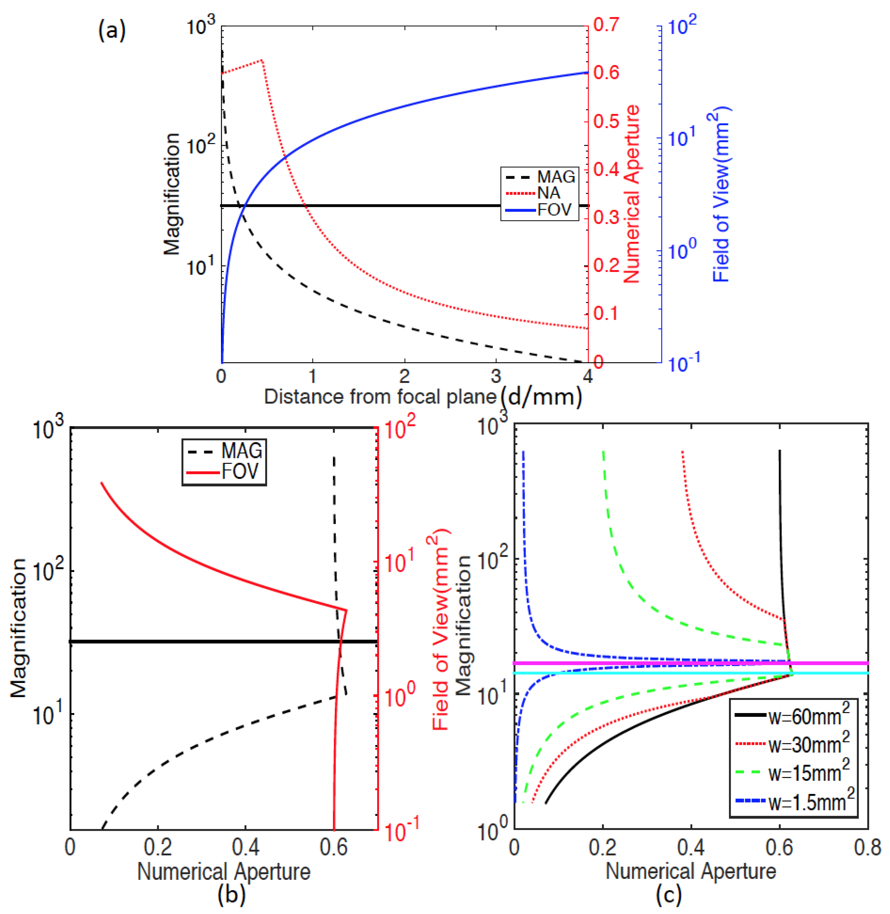
5. Numerical Aperture, Field-of-View, Magnification

The magnification of the system is determined by the position of the sample relative to the focused spot, and is given in Equation (3). A simple inspection of this equation reveals that the largest magnification that is achievable is infinity, M m a x = , which occurs when the sample is placed in the same plane as the point source, i.e., when d = 0 . The smallest magnification that is achievable occurs when the sample is placed as close as possible to the MO, i.e., at the largest possible value of d. The working distance, W D , of the MO will in general be shorter than the focal length of the MO, f. Therefore, the smallest magnification is given by:
M m i n = f f W D
which will always be greater than one. The ratio of the working distance to focal length varies significantly across microscope objectives. For the long working distance used in this study, the value of M m i n 2 . Using the value of M, it is also possible to calculate the Field-of-View, F o V , of the resultant image by simply dividing the sensor dimensions, w x and w y , by the magnification to provide (assuming the wavefield overfills the sensor area):
F o V = ( w x × w y ) / M 2
For the MO used in this study, the value for F o V will vary from 0, for the case of M m a x to ( w x × w y ) / 4 for the case of M m i n , i.e., it should be possible to record a Field-of-View approximately equal to one quarter of the area of the recording sensor. In Figure 4a the magnification and Field-of-View are both shown as a function of the sample position d. The MO used in this study has a Numerical Aperture of 0.6, a focal length of f = 6.25 mm and a working distance of 3.5 mm. The range of values of d over which the parameters M and F o V are calculated is from 0 mm up to 4 mm. It can be seen that M decreases rapidly from infinity at d = 0 to a value of M = 7 over the first 1 mm from the point source, while F o V increases rapidly over this range.
Although it is straightforward to define the magnification and Field-of-View as a function of sample positions, it is not immediately obvious how to define the Numerical Aperture of the imaging system. It can be expected that the NA will vary depending on the position of the sample plane relative to the MO, since this will change the angle that subtends the center of the object on the optical axis, to the edge of the MO. However, the rays that propagate at the most extreme angles into the MO, might not be captured by the apertures of one or more of the remaining optical elements. Therefore, in order to determine the NA for a given sample position, d, it is necessary to perform ray-tracing using the matrices for each of the optical elements in the system and to take into account the aperture of each optical element. This can be done systematically, such that for the center point on the sample, the maximum ray angle can be determined that will pass through each individual element and reach the detector. As an example, consider the tube lens T L in the setup. The position, x and angle θ of a ray that originates at the center of the sample (position x = 0 ) propagating at an angle θ can be calculated as follows [20]:
x cos 1 θ = M 2 M 1 0 cos 1 θ
Therefore, the position of the ray in the plane of the tube lens is given by:
x = B cos 1 θ
where B is the parameter from the A B C D ray-transfer matrix that is given by M 2 M 1 . The maximum value of x is given by the radius of the tube lens and in this way, the maximum ray angle from the sample center that can pass through the tube lens can be calculated. The same procedure can be applied for the third lens in the system f F T and for the sensor; the position of the ray in these two planes is also given by Equation (7) where the B parameters is taken from the two matrix products, M 6 M 5 M 4 M 3 M 2 M 1 and M 8 M 7 M 6 M 5 M 4 M 3 M 2 M 1 respectively. In practice, for the components used in this study, it was found that, in addition to the aperture of the MO, the limiting aperture was in general defined by the sensor aperture. The Numerical Aperture is also plotted as a function of sample position, d, in Figure 4a, in which it is predicted that the designed NA of the MO (0.6) can be approximately achieved for a range of different magnifications and FoVs. At a distance of d = 0.2 mm, the magnification of the system is predicted to be M = 32 , which is marked by a horizontal line in the figure; interestingly, this is the intended magnification of the MO, and at this position the NA is estimated to be slightly greater than the design value of 0.6 when used in the typical microscope configuration. From a position of d = 0.5 mm, corresponding to a magnification of M = 10 , the NA begins to drop rapidly as the value of d increases. At a value of d = f , which corresponds to a magnification of M = 1 , it can be seen that the NA has dropped to a value of 0.07 . In Figure 4b M and F o V are both plotted as a function of the Numerical Aperture. It can be seen that for a range of different magnifications, from 10 < M < the maximum NA of approximately 0.6 is predicted by this model. Below a value of M = 10 the NA drops in an approximately linear manner as a function of magnification. Conversely, the F o V decreases approximately linearly for values of 0.0 < NA < 0.6 . It was found that the sensor aperture played an important role in defining the relationship between the NA and the value of M; this relationship is illustrated in Figure 4c for a range of different square sensor area w mm 2 , where all other parameters are the same as those already defined. For the smallest sensor area investigated, w = 1.5 mm 2 it can be seen that the maximum NA of 0.6 can only be achieved for a particular sample position corresponding to a magnification of M = 10.8 denoted by the pink line in the figure. Deviation from this position to provide any other magnification is predicted to result in a sharp decrease in NA. This constraint relaxes as the sensor area is increased in the sense that the range of values of M that can provide the maximum NA widens as a function of w.

6. Preliminary Results Using a Micro-Lens Array

The results are shown for a micro array sample (SUSS MLA 18-00028 quartz, circ. lenses, quad. grid, pitch 110 μ m, ROC 6.188 mm ± 5 % , size 10 mm × 10 mm ± 0.05 mm , thickness 0.9 mm ). The sample was placed in a range of different positions and the results are shown in Figure 5 for three different values of d corresponding to magnifications of M = 32 , which is the design magnification of the MO, M = 12 , and M = 5 .
The reconstructed intensity and phase images are shown for the three cases in Figure 5a–f following spatial filtering with the DFT to isolate the real image, followed by simulation of Fresnel propagation of distance q using the spectral method as discussed in the previous sections. For the phase images shown in Figure 5d–f no attempt is made to perform aberration compensation. The sample position d is shown in the top right corner of each intensity image, and the values of NA and F o V are also shown in each intensity image, which have been calculated using the formula defined in Section 4 and Section 5.
The same set of results are shown in Figure 5g–i where in this case aberration compensation is applied using the method described in ref. [28], which makes use of a reference conjugated hologram. This form of aberration compensation is relatively simple, whereby a reference hologram is recorded with no sample, and the resulting complex hologram is divided into the hologram of the object prior to reconstruction. Although this attempt to compensate for aberrations clearly improves the phase image, it only partially corrects for overall aberration. The clear distortion in the intensity image (which should have approximately uniform amplitude) resulting from system aberration remain in the image. Unfortunately, it is not possible at this time to confirm the Numerical Aperture of the system experimentally for a range of magnifications due to the presence of this distortion.

7. Discussion

7.1. Aberration

Although the simple method of using a conjugated reference hologram did improve the phase aberration in the reconstructed image, there remained significant image distortion. Of particular concern is the fact that the MO is being used to image a sample that is placed far from the working distance at which the MO was designed to image, resulting in the projection of the image onto a curved surface. Additionally, of concern is the fact that the aberrations from two different microscope objectives are contributing to image distortion. The condenser is expected to produce an ideal diverging spherical wavefront (that we model as an ideal thin lens) at the sample plane, which will in practice contain aberrations which will also contribute to aberration in the image. Our initial results indicate that traditional methods of aberration compensation fail [28,29,30,31]. Additionally, recording holograms of point-source pinhole objects in order to determine the aberration in the image, which have been shown to be highly successful in aberration compensation for other DHM systems [32], indicate that the aberration is not spatially invariant across the sample plane; i.e., the aberration for a point in the centre of the object is different that for a point further away. Therefore, attempting to solve the problem of aberration using holograms of point sources becomes intractable considering that holograms would have to be applied from pinholes at every possible three-dimensional position that could be occupied by a sample, followed by a spatially variant convolution operation. It is likely that the projection of the image onto a curved surface is at the source of this problem and finding a method to fully compensate for the aberrations will be an important part of future work in order to move this work from a proof-of-concept to a reliable and usable tool for the life-science community.

7.2. Relationship of the Proposed System to Off-Axis DIHM

Recently the digital in-line holographic microscopy approach has been augmented with an off-axis reference beam that can separate the twin images and accurately retrieve the phase [33,34]. This approach uses two closely situated point sources, whereby one point source illuminates the object and the second provides the reference. Although this work is similar to our own in terms of providing off-axis holographic microscopy with variable magnification by moving the sample, there are some important differences: (i) Our proposed system is a simple adaptation of the common off-axis architecture. Lenless point-source methods such as those in [33,34] are limited in terms of Numerical Aperture/resolution by the absence of a high quality microscope objective and immersion medium; (ii) The double point sources method places a constraint on the sample whereby features within the sample cannot overlap with the reference point source path. Our system has no such limitation. For typical glass slides used in life-science, the microscopist will commonly wish to view a densely populated sample area of several cm 2 .

7.3. Laser Source

The type of laser used in the proposed setup is an interesting point of discussion. In recent years, there has been a shift away from sources with high-temporal coherence, which produce coherent noise in the image from scattering and reflections at various points in the optical system, towards laser sources with relatively short coherent lengths. The source used in this study is a relatively inexpensive laser diode (EUR 1k) with a bandwidth of approximately 1 nm and a coherence length of approximately 0.1 mm. Despite the short coherence length, it is straight forward to match the path lengths in the Mach-Zender architecture that is used in this study using a lens tube mounted on a cage-optics translation stage. The use of sources with larger bandwidths has been shown to produce very low noise phase images: a supercontinuum laser source with FWHM of 6.7 nm is used in a Michelson DHM setup in ref. [35], a filtered Zenon lamp with a bandwidth of 5 nm is used in the DIHM setup in ref. [36]. This latter system has also been demonstrated with filtered LED illumination. LED or Zenon illumination would not be suitable for the system proposed here, due to the requirement for high spatial coherence in the object and reference wavefields. However, it is likely that a supercontinuum laser with a bandwidth >1 nm would produce lower-noise images. The cost of such laser systems is, however, very high and we believe that the use of inexpensive diodes provides a benefit in terms of image quality and cost. It is likely that battery powered laser diodes costing <EUR 10 could be used with the proposed setup.

8. Conclusions

In conclusion, this letter outlines a novel architecture for off-axis digital holographic microscopy that has the capability to provide for continuously variable magnification over a range of values from approximately two times up to infinity, by simply moving the position of the sample in the setup along the optical axis. The experimental system, which comprises a small adaptation of a traditional setup for off-axis holographic microscopy, is described in detail and the ray-transfer matrix for the system is used to derive the relationship between the sample plane and the sensor plane. It is shown that this mapping reduces to a single magnification step and a Fresnel transform. The ray-transfer matrix of each component in the setup is used to calculate the largest angle of light from the center of the sample that could be recorded by the sensor, and in this way the Numerical Aperture of the system for each sample position and magnification is estimated. The preliminary experimental results clearly demonstrate a proof-of-concept implementation of the method by imaging a micro-lens array over a range of magnifications and Field-of-View.
The proposed method is compared directly with DIHM, which is a digital implementation of Gabor’s original invention. It is shown using the ray-transfer matrix that the principle of variable magnification for the proposed system is identical to the case of DIHM. Unlike DIHM, however, the proposed system produces quantitative phase images in a single capture and requires no preconditions on a weakly scattering object. An important consideration is that the proposed method will provide a large range of magnification only if there is a large working distance, i.e., a large range of travel in front of the microscope objective. This feature is provided by long working distance objectives such as the one used in this study. Microscope objectives with even longer working distances are available from other sources such as Mitutoyo and it will be interesting to see if other researchers investigate their potential in future work.
A significant shortcoming of the method is the manifestation of aberrations in the reconstructed image. These have been partially compensated using reference conjugate hologram that is applied in the hologram plane. Other more complicated methods, which are highly effective when imaging in the traditional object plane using off-axis DHM, appear to fail for the system proposed here; this problem appears to result from the projection of the recorded hologram onto a curved surface owing to the short distance between the sample and the MO. A more effective method of aberration compensation must be developed in order to ensure the usefulness of the method for practical applications.

Author Contributions

Conceptualization, X.F. and B.M.H.; methodology, X.F., B.M.H., K.O.; formal analysis, X.F., B.M.H., J.J.H., K.O., J.W.; resources, B.M.H.; writing—original draft preparation, X.F., B.M.H.; writing—review and editing, X.F., B.M.H., K.O., J.J.H., J.W.; supervision, B.M.H., K.O.; project administration, B.M.H.; funding acquisition, B.M.H. All authors have read and agreed to the published version of the manuscript.

Funding

This research was conducted in part with the financial support of Science Foundation Ireland (SFI) under Grant numbers 18/TIDA/6156 and 15/CDA/3667. John Healy acknowledges the support of the Irish Research Council and the National University of Ireland. Xin Fan, acknowledges the support of the John & Pat Hume Scholarship. Julianna Winnik acknowledges the support of the National Science Centre, Poland under Grant Number 2015/17/B/ST8/02220.

Institutional Review Board Statement

Not applicable.

Informed Consent Statement

Not applicable.

Conflicts of Interest

The authors declare no conflict of interest. The funders had no role in the design of the study; in the collection, analyses, or interpretation of data; in the writing of the manuscript, or in the decision to publish the results.

Appendix A. The Ray Transfer Matrix and Its Relationship to Wave Optics

In this subsection, we briefly review the concept of the ray transfer matrix, also known as the A B C D ray transfer matrix, which can be used to trace the direction and position of a geometrical ray as it pass through an optical system [20]. Each optical element in a complex optical system, including a section of free space, can be assigned an A B C D matrix. The overall A B C D ray transfer matrix for the entire system is given by the product of these individual matrices in the order in which they act on the input ray. The A B C D matrix is applied in Section 4 and Section 5 in order to: (i) to identify a suitable reconstruction algorithm for a novel digital holographic microscopy optical system and (ii) to estimate the magnification, Numerical Aperture, and Field-of-View of the system by tracing rays through the optical components and identifying the maximum ray angle from the object that can be captured by the recording camera. In order to illustrate the concept of the ray transfer matrix we must first familiarise ourselves with simple examples that form the of analysis in Appendix B as well as Section 4 and Section 5 in the main body of the paper:
A B C D = 1 z 0 1 ,
A B C D = M 0 0 1 / M ,
A B C D = 0 1 1 0 ,
and A B C D = 1 0 1 / f 1 .
These four matrices represent the A B C D ray transfer matrices for (i) propagation in free space (equivalent to a Fresnel transform acting on a complex wavefield in the paraxial approximation), (ii) a magnification system (scaling), (iii) a Fourier transform and (iv) a ‘thin’-lens [20], where z is the propagation distance, M is a magnification factor and f is the focal length of the lens [20,37]. It has been shown by Collins [37] that using the paraxial approximation, the integral transformation that models the diffraction between the input and output planes of the system, is given by the following equation:
F A B C D { g ( x ) } ( x ) = 1 i λ B + g x exp i π A x 2 2 x x + D x 2 λ B d x .
This integral relationship is known as the Linear Canonical Transform [38], where λ is the wavelength, x , and x represent the input and output coordinate systems. Substituting the A,B,C, and D parameters for free space propagation into Equation (A5) produces the Fresnel transform, which is explicitly defined in the next subsection. Using this simple relationship between geometrical optics and wave-optics it is possible to quickly define the integral transformation associated with any optical system by firstly calculating the overall A B C D matrix. We refer the reader to references [25,39,40] for a graphical interpretation of the effect of these matrices in Phase-Space. We also note that in ref. [25] a method for designing new algorithms associated with the discrete counterparts of the integral transformation is provided. For simplicity, we consider the one-dimensional case only.

Appendix B. Digital In-Line Holographic Microscopy and Variable Magnification

In this section, we briefly review the principles of DIHM, which form the basis for modelling the experimental system described in Section 2.1. In a DIHM recording system, an object is illuminated by a diverging spherical wave, usually originating from a small pinhole. The object scatters some of the light, thereby creating the object wave. Assuming the object is weakly scattering, the undiffracted light provides the reference wave. A typical setup for DIHM is shown in Figure A1. A spherical wave emerges from a pinhole with a wavelength λ . Following propagation of a distance d, this diverging spherical wavefield is incident upon a weakly scattering object with a transmission function approximated by [20]:
t ( x ) 1 + o ( x ) .
where the amplitude and phase of o ( x ) represent the absorption and phase-delay imparted by the object on the illumination. An intensity pattern is recorded from the resultant wavefield a further distance z away from the object plane.
Figure A1. Gabor DIHM setup with a spherically diverging beam, r ( x ) , emerging from a pinhole, illuminating a weakly scattering object with transmittance, t ( x ) = 1 + o ( x ) , a distance d away. Immediately behind this plane there is the object wavefield o ( x ) r d ( x ) , where the subscript d denotes the radius of the spherical wave in this plane. The interference pattern, between the unscattered component, r f ( x ) , and the propagated object wave, O ( x ) , is captured on a CCD a further d 2 away. The captured intensity is input to a numerical reconstruction algorithm.
Photonics 08 00264 g0a1
The diverging spherical wavefield from the point source can be described using Phasor notation in both the object plane, r d ( x ) , and the camera plane, r f ( x ) , as follows:
r d ( x ) = exp i π x 2 λ d r f ( x ) = exp i π x 2 λ f
where f = z + d . The field in the plane immediately after the object plane can, be described as r d ( x ) + r d ( x ) o ( x ) , i.e., the product of the illuminating spherical wavefield and the transmittance. Following a Fresnel propagation, the field in the camera plane can be described as O ( x ) + r f ( x ) , where O ( x ) represents the propagated object field as follows:
O ( x ) = F z o ( x ) r d ( x ) x = F z o ( x ) exp i π x 2 λ d x
and where F z denotes the operator for the Fresnel Transform, which is defined in the equation below:
F z { g ( x ) } x = 1 i λ z + g ( x ) exp i π [ x x ] 2 λ z d x
Using the properties of the Fresnel transform [8], it is possible to rewrite Equation (A8) as follows:
O ( x ) = exp i π x 2 λ d M F M z o x M x
where M = d / ( d + z ) = d / f . This indicates that the effect of illuminating the sample o ( x ) with a diverging spherical wavefield (with parameter d) followed by propagation of distance z is equivalent to first magnifying the sample o ( x ) by a factor M, followed by propagation a distance M z , followed by multiplying the result by a chirp function with parameter d M . This result can be confirmed using the following matrix decomposition:
1 z 0 1 1 0 1 / d 1 = 1 0 1 / M d 1 1 M z 0 1 M 0 0 1 / M
The matrices on the left of the equals sign in the above equation relate to Equation (A8), while the matrices on the right side relate to Equation (A10) based on the principles described in Appendix A. It is straightforward to show that the relationship in Equation (A11) is true if M = d / ( d + z ) .
If the complex valued O ( x ) can be retrieved from the recorded intensity pattern on the camera, the magnified image o ( x / M ) can be numerically reconstructed by firstly multiplying by a discrete chirp function with parameter d M followed by computation of the Fresnel transform a distance z M . Several algorithms have been developed for reconstruction that make use of this matrix decomposition [7] as well as others. However, it is not straightforward to recover O ( x ) in isolation from the recorded intensity pattern, which is given by:
I i n l i n e ( x ) = O ( x ) + r f ( x ) 2
which can be expanded to produce an expression with four terms:
I i n l i n e ( x ) = | O ( x ) | 2 + | r f ( x ) | 2 + O ( x ) r f * ( x ) + r f ( x ) O * ( x ) .
The limitations of DIHM systems in terms of magnification, Numerical Aperture, and Field-of-View have been investigated extensively by other authors [11,12,13,14]. Despite the attempts to remove or ignore the three unwanted terms in Equation (A12), their residual effect is to render the phase image unusable. Numerical techniques have been developed that have improved the quality of the phase image based on iteratively numerically propagating between the camera and object plane and applying a set of constraints in both of these planes [41]. While this technique does improve the phase image it does not, in general, work well for all samples.
Another approach is to record the hologram for several different sample positions, i.e., for several values of d in Figure A1, and to either use an iterative constraint based approach or the transport of intensity equation or both in order to recover meaningful phase images [21,22]. Yet another recent approach [42] scans the wavelength of the illumination over a range of values; a sequence of intensity images is recorded and an accurate phase image can be recovered.
All of these multi-capture methods, while recovering an accurate phase image, have the obvious disadvantage of requiring several recordings and significant computation. Another class of related methods is the double point source approach [33,34], which uses two closely situated point sources, whereby one point source illuminates the object and the second provides the reference. Like the method proposed in this paper, the approach separates the twin images using an off-axis reference wavefield. The relationship between the method proposed in this paper, and the double point-source method is further discussed in Section 7.2.

References

  1. Gabor, D. A new microscopic principle. Nature 1948, 161, 777–778. [Google Scholar] [CrossRef]
  2. Leith, E.N.; Upatnieks, J. Wavefront reconstruction with diffused illumination and three-dimensional objects. Josa 1964, 54, 1295–1301. [Google Scholar] [CrossRef]
  3. Kreis, T.M. Handbook of Holographic Interferometry; Wiley-VCH: Weinheim, Germany, 2005. [Google Scholar]
  4. Schnars, U.; Jüptner, W.P.O. Digital Holography; Springer: Berlin/Heidelberg, Germany, 2004. [Google Scholar]
  5. Cuche, E.; Marquet, P.; Depeursinge, C. Spatial filtering for zero-order and twin-image elimination in digital off-axis holography. Appl. Opt. 2000, 39, 4070–4075. [Google Scholar] [CrossRef] [PubMed]
  6. Kim, M.K. Digital holographic microscopy. In Digital Holographic Microscopy; Springer: Berlin/Heidelberg, Germany, 2011; pp. 149–190. [Google Scholar]
  7. Molony, K.M.; Hennelly, B.M.; Kelly, D.P.; Naughton, T.J. Reconstruction algorithms applied to in-line Gabor digital holographic microscopy. Opt. Commun. 2010, 283, 903–909. [Google Scholar] [CrossRef] [Green Version]
  8. Hennelly, B.M.; Kelly, D.P.; Monaghan, D.S.; Pandey, N. Zoom algorithms for digital holography. In Information Optics and Photonics; Springer: Berlin/Heidelberg, Germany, 2010; pp. 187–204. [Google Scholar]
  9. Kemper, B.; von Bally, G. Digital holographic microscopy for live cell applications and technical inspection. Appl. Opt. 2008, 47, A52–A61. [Google Scholar] [CrossRef]
  10. Fan, X.; Healy, J.J.; O’Dwyer, K.; Hennelly, B.M. Label-free color staining of quantitative phase images of biological cells by simulated Rheinberg illumination. Appl. Opt. 2019, 58, 3104–3114. [Google Scholar] [CrossRef] [PubMed]
  11. Garcia-Sucerquia, J.; Xu, W.; Jericho, S.K.; Klages, P.; Jericho, M.H.; Kreuzer, H.J. Digital in-line holographic microscopy. Appl. Opt. 2006, 45, 836–850. [Google Scholar] [CrossRef] [PubMed]
  12. Garcia-Sucerquia, J.; Xu, W.; Jericho, M.; Kreuzer, H.J. Immersion digital in-line holographic microscopy. Opt. Lett. 2006, 31, 1211–1213. [Google Scholar] [CrossRef]
  13. Jericho, S.; Garcia-Sucerquia, J.; Xu, W.; Jericho, M.; Kreuzer, H. Submersible digital in-line holographic microscope. Rev. Sci. Instrum. 2006, 77, 043706. [Google Scholar] [CrossRef]
  14. Garcia-Sucerquia, J. Color lensless digital holographic microscopy with micrometer resolution. Opt. Lett. 2012, 37, 1724–1726. [Google Scholar] [CrossRef] [PubMed]
  15. Jericho, M.; Kreuzer, H.; Kanka, M.; Riesenberg, R. Quantitative phase and refractive index measurements with point-source digital in-line holographic microscopy. Appl. Opt. 2012, 51, 1503–1515. [Google Scholar] [CrossRef]
  16. Kreuzer, H.J. Holographic Microscope and Method of Hologram Reconstruction. U.S. Patent 6,411,406, 25 June 2002. [Google Scholar]
  17. Luo, W.; Zhang, Y.; Göröcs, Z.; Feizi, A.; Ozcan, A. Propagation phasor approach for holographic image reconstruction. Sci. Rep. 2016, 6, 22738. [Google Scholar] [CrossRef]
  18. Ozcan, A.; Greenbaum, A. Maskless Imaging of Dense Samples Using Multi-Height Lensfree Microscope. U.S. Patent 9,715,099, 25 July 2017. [Google Scholar]
  19. Rivenson, Y.; Zhang, Y.; Günaydın, H.; Teng, D.; Ozcan, A. Phase recovery and holographic image reconstruction using deep learning in neural networks. Light. Sci. Appl. 2018, 7, 17141. [Google Scholar] [CrossRef]
  20. Goodman, J.W. Introduction to Fourier Optics; Roberts & Company Publishers: Greenwood Village, CO, USA, 2004. [Google Scholar]
  21. Greenbaum, A.; Ozcan, A. Maskless imaging of dense samples using pixel super-resolution based multi-height lensfree on-chip microscopy. Opt. Express 2012, 20, 3129–3143. [Google Scholar] [CrossRef]
  22. Waller, L.; Luo, Y.; Yang, S.Y.; Barbastathis, G. Transport of intensity phase imaging in a volume holographic microscope. Opt. Lett. 2010, 35, 2961–2963. [Google Scholar] [CrossRef]
  23. Fan, X.; Healy, J.J.; Hennelly, B.M. Investigation of sparsity metrics for autofocusing in digital holographic microscopy. Opt. Eng. 2017, 56, 053112. [Google Scholar] [CrossRef]
  24. Rhodes, W.T. Light Tubes, Wigner Diagrams, and Optical Wave Propagation Simulation. In Optical Information Processing: A Tribute to Adolf Lohmann; SPIE Press: Bellingham, WA, USA, 2002; p. 343. [Google Scholar]
  25. Hennelly, B.M.; Sheridan, J.T. Generalizing, optimizing, and inventing numerical algorithms for the fractional Fourier, Fresnel, and linear canonical transforms. JOSA A 2005, 22, 917–927. [Google Scholar] [CrossRef] [PubMed] [Green Version]
  26. Mendlovic, D.; Zalevsky, Z.; Konforti, N. Computation considerations and fast algorithms for calculating the diffraction integral. J. Mod. Opt. 1997, 44, 407–414. [Google Scholar] [CrossRef]
  27. Memmolo, P.; Distante, C.; Paturzo, M.; Finizio, A.; Ferraro, P.; Javidi, B. Automatic focusing in digital holography and its application to stretched holograms. Opt. Lett. 2011, 36, 1945–1947. [Google Scholar] [CrossRef] [PubMed]
  28. Colomb, T.; Kühn, J.; Charriere, F.; Depeursinge, C.; Marquet, P.; Aspert, N. Total aberrations compensation in digital holographic microscopy with a reference conjugated hologram. Opt. Express 2006, 14, 4300–4306. [Google Scholar] [CrossRef] [PubMed]
  29. Colomb, T.; Cuche, E.; Charrière, F.; Kühn, J.; Aspert, N.; Montfort, F.; Marquet, P.; Depeursinge, C. Automatic procedure for aberration compensation in digital holographic microscopy and applications to specimen shape compensation. Appl. Opt. 2006, 45, 851–863. [Google Scholar] [CrossRef] [Green Version]
  30. Colomb, T.; Montfort, F.; Kühn, J.; Aspert, N.; Cuche, E.; Marian, A.; Charrière, F.; Bourquin, S.; Marquet, P.; Depeursinge, C. Numerical parametric lens for shifting, magnification, and complete aberration compensation in digital holographic microscopy. JOSA A 2006, 23, 3177–3190. [Google Scholar] [CrossRef]
  31. Ferraro, P.; De Nicola, S.; Finizio, A.; Coppola, G.; Grilli, S.; Magro, C.; Pierattini, G. Compensation of the inherent wave front curvature in digital holographic coherent microscopy for quantitative phase-contrast imaging. Appl. Opt. 2003, 42, 1938–1946. [Google Scholar] [CrossRef]
  32. Cotte, Y.; Toy, F.; Jourdain, P.; Pavillon, N.; Boss, D.; Magistretti, P.; Marquet, P.; Depeursinge, C. Marker-free phase nanoscopy. Nat. Photonics 2013, 7, 113–117. [Google Scholar] [CrossRef]
  33. Serabyn, E.; Liewer, K.; Wallace, J. Resolution optimization of an off-axis lensless digital holographic microscope. Appl. Opt. 2018, 57, A172–A180. [Google Scholar] [CrossRef] [PubMed]
  34. Serabyn, E.; Liewer, K.; Lindensmith, C.; Wallace, K.; Nadeau, J. Compact, lensless digital holographic microscope for remote microbiology. Opt. Express 2016, 24, 28540–28548. [Google Scholar] [CrossRef]
  35. Girshovitz, P.; Shaked, N.T. Compact and portable low-coherence interferometer with off-axis geometry for quantitative phase microscopy and nanoscopy. Opt. Express 2013, 21, 5701–5714. [Google Scholar] [CrossRef] [PubMed] [Green Version]
  36. Bishara, W.; Su, T.W.; Coskun, A.F.; Ozcan, A. Lensfree on-chip microscopy over a wide field-of-view using pixel super-resolution. Opt. Express 2010, 18, 11181–11191. [Google Scholar] [CrossRef] [PubMed]
  37. Collins, S.A. Lens-system diffraction integral written in terms of matrix optics. JOSA 1970, 60, 1168–1177. [Google Scholar] [CrossRef]
  38. Healy, J.J.; Kutay, M.A.; Ozaktas, H.M.; Sheridan, J.T. Linear Canonical Transforms: Theory and Applications; Springer: Berlin/Heidelberg, Germany, 2015; Volume 198. [Google Scholar]
  39. Sheridan, J.T.; Hennelly, B.M.; Kelly, D.P. Motion detection, the Wigner distribution function, and the optical fractional Fourier transform. Opt. Lett. 2003, 28, 884–886. [Google Scholar] [CrossRef] [Green Version]
  40. Kelly, D.P.; Hennelly, B.M.; Rhodes, W.T.; Sheridan, J.T. Analytical and numerical analysis of linear optical systems. Opt. Eng. 2006, 45, 088201-1–088201-12. [Google Scholar] [CrossRef]
  41. Latychevskaia, T.; Fink, H.W. Solution to the twin image problem in holography. Phys. Rev. Lett. 2007, 98, 233901. [Google Scholar] [CrossRef] [PubMed] [Green Version]
  42. Wu, X.; Sun, J.; Zhang, J.; Lu, L.; Chen, R.; Chen, Q.; Zuo, C. Wavelength-scanning lensfree on-chip microscopy for wide-field pixel-super-resolved quantitative phase imaging. Opt. Lett. 2021, 46, 2023–2026. [Google Scholar] [CrossRef] [PubMed]
Figure 1. Optical setup of variable magnification off-axis DHM. L: Plano-convex lens; FC: Fiber Coupler; FS: Fiber Splitter; P: Polarizer; C: condenser; S: Sample plane; MO: Microscope Object; TL: Tube Lens; PBS: Beam Splitter; FL: Fourier transforming convex lens. The dashed lines represent the typical object plane at the focal plane of the (infinity corrected) MO and the corresponding image plane; also for typical DHM the illumination would be a plane wave whereas for this setup the illumination is a diverging spherical wave originating from a point-source at the focal plane, which is produced via beam-focusing using the condenser lens. The object can be placed anywhere between the focal plane of the MO and the surface of the MO to achieve variable magnification. Another feature of the setup is that instead of recording the complex wavefield at the image plane of the microscope, the optical Fourier transform of this image is recorded by inserting a lens after the image plane.
Photonics 08 00264 g001
Figure 2. A simplified schematic that corresponds to the optical system proposed in Section 2.1, which can be compared directly to the traditional DIHM set up illustrated in Figure A1. In this case, an MO (positioned a focal length away from the point-source) captures the wavefield in lieu of the camera and effectively collimates the wavefield into an off-axis interferometer. There is no requirement on the object to be weakly scattering and hence the propagated field is denoted a function of t ( x ) and not o ( x ) as for DIHM. Note the surface of the MO will be closer than the effective lens plane, and this working distance (WD) places a greater constraint on the range of sample placement relative to the case of DIHM. In both cases the magnification (M) of the imaging system is the same.
Photonics 08 00264 g002
Figure 3. Illustration of the optical system that maps the input sample plane to the output camera plane; S, Sample; C, Complex lens; MO, Microscope objective; TL, Tube lens; L, Fourier transforming convex lens. Here, the divergent spherical illumination is represented as a convex lens of focal length d in the plane immediately after the sample plane and coherent plane wave illumination is assumed.
Photonics 08 00264 g003
Figure 4. The relationships between magnification, Field-of-View and Numerical Aperture for the setup shown in Figure 1; (a) shows the variation in M, F o V , and N A as a function of sample position d in the setup; (b) M and F o V are both plotted as a function of N A ; and (c) the relationship between M and N A is shown for a range of different sensor areas, w = w x × w y .
Photonics 08 00264 g004
Figure 5. Raw amplitude and wrapped phase images of micro-lens array for different magnifications. (ac) show the reconstructed intensity for magnifications of 32, 12, and 5, respectively. Parts (df) show the corresponding phase image, and (gi) show the same phase images following basic aberration compensation using a conjugated reference hologram as described in the text.
Photonics 08 00264 g005
Publisher’s Note: MDPI stays neutral with regard to jurisdictional claims in published maps and institutional affiliations.

