Article

Dynamic Speckle Illumination Digital Holographic Microscopy by Doubly Scattered System

1
Key Lab of NC Machine Tools and Integrated Manufacturing Equipment of the Education Ministry & Key Lab of Mechanical Manufacturing Equipment of Shaanxi Province, Xi’an University of Technology, Xi’an 710048, China
2
School of Mechanical and Precision Instrument Engineering, Xi’an University of Technology, Xi’an 710048, China
*
Author to whom correspondence should be addressed.
Photonics 2021, 8(7), 276; https://doi.org/10.3390/photonics8070276
Submission received: 10 June 2021 / Revised: 10 July 2021 / Accepted: 11 July 2021 / Published: 14 July 2021
(This article belongs to the Special Issue Holography)

Abstract

:
The coherent noise always exists in digital holographic microscopy due to the laser source, degrading the image quality. A method of speckle suppression using the dynamic speckle illumination, produced by double-moving diffusers, is presented in digital holographic microscopy. The space–time correlation functions are theoretically analyzed from the statistics distribution in the doubly and singly scattered system, respectively. The configuration of double-moving diffusers is demonstrated to have better performance in speckle suppression compared with the single diffuser and moving-static double diffusers cases. The experiment results verify the feasibility of the approach. The presented approach only requires a single shot interferogram to realize the speckle reduction, accordingly it has the potential application in real-time measurement.

1. Introduction

Digital holographic microscopy is a powerful technique for quantitatively measuring the three-dimensional (3D) morphology of transparent samples such as biological cells [1,2,3]. The laser source, as a coherent illumination, causes the holographic imaging to suffer from the coherent noise. The coherent noise or grain speckle is mainly introduced by undesired diffraction and multiple reflections from the dust particles, scratches and defects on and in the optical elements, thus seriously degrading the imaging quality [4].
The typical speckle suppression uses a temporal integration of different speckle patterns. These multiple holograms with uncorrelated speckle patterns may be obtained by using illumination angle diversity [5,6], wavelength diversity [7], polarizations diversity [8,9], shifting object [10] or hologram aperture [11], and rotating diffuser [12,13]. Among these, the speckle illumination through rotating diffusers is often employed due to its simplicity, in which the shorter spatial coherence length can prevent the interference caused by unwanted diffractions [12,13,14,15,16,17]. The static or dynamic speckle illumination has been studied to reduce coherent noise in the last few years. The static speckle illumination, however, performs multiple measurements to retrieve high quality imaging [14], thus restricting its application in the dynamic measurement. The dynamic speckle field illumination through single moving diffuser [15,16] or double diffusers with a static and a moving state [17] only requires a single shot recording to realize the coherent speckle suppression.
In the paper, a dynamic speckle illumination coupled with double-moving diffusers is proposed in digital holographic microscopy. When the double diffusers are rotated fast enough within the camera exposure time, large number of speckle patterns can be generated during the single acquisition. The spatial correlation properties and the temporal correlation properties are analyzed theoretically from the space–time correlation function of double diffusers and single diffuser, respectively. It is demonstrated by the results of simulations and experiments that the doubly scattered system, made up of two moving diffusers, provides better speckle suppression performance compared with the single diffuser or moving-static double diffusers system.

2. Theoretical Analyses

2.1. Space–Time Correlation Function

The transmitted light fields are scattered twice in the doubly scattered system. The speckle fields induced on the observation plane obeys K-distributed or Gaussian-distributed statistics in the certain condition. The optical schematic of rotating double diffusers is illustrated in Figure 1. D1 and D2 are two diffusers around the optical axis with angular speeds of ω 1 and ω 2 , respectively. A laser, with 1/e2 intensity radius of w0 and wavelength λ , is scattered by two diffusers apart from distance d. Then the scattered fields are imaged onto the observation plane through a thin lens with diameter 2a0 and focal length f, i.e., 1 / f = 1 / d i + 1 / d o . When speckle fields obey K distribution in the doubly scattered system, the space–time correlation function of the speckle intensity at the observation plane is derived as [18]:
I ( p 1 , t ) I ( p 2 , t + τ ) = Γ 0 + Γ 1 ( p 1 , p 2 , ω 1 τ , υ ) + Γ 2 ( p 1 , p 2 , ω 2 τ , υ ) + Γ 12 ( p 1 , p 2 , ω 1 τ , ω 2 τ , υ )
where the angled brackets denote an ensemble average, I(p,t) is the speckle intensity at position p and time t, τ is the time difference between the captures of the two intensities. The Γ0, Γ1, Γ2 and Γ12 are expressed as in Equation (1a), respectively:
Γ 0 = π 2 ρ 1 4 4
Γ 1 = π 2 ρ 1 4 4 υ exp [ ( 1 υ ) ( p 2 p 1 cos ω 1 τ + p 1 sin ω 1 τ ) 2 ρ 2 2 ]
Γ 2 = π 2 ρ 1 4 4 υ exp [ ( p 2 p 1 cos ω 2 τ + p 1 sin ω 1 τ ) 2 ρ 2 2 ]
Γ 12 = π 2 ρ 1 4 υ 2 [ 1 + υ ( 1 υ ) cos ( ω 1 τ ω 2 τ ) ] 2 × exp { 2 υ ( p 2 p 1 cos ω 2 τ + p 1 sin ω 2 τ ) 2 ρ 2 2 [ 1 + υ ( 1 υ ) cos ( ω 1 τ ω 2 τ ) ] } × exp { 2 ( 1 υ ) [ 1 cos ( ω 1 τ ω 2 τ ) ] ( p 1 2 + p 2 2 ) ρ 2 2 [ 1 + υ ( 1 υ ) cos ( ω 1 τ ω 2 τ ) ] }
Speckle intensity consists of four terms. Γ0 is a constant term. Γ1 and Γ2 represent the separable effects arising from D1 and D2, respectively. They are either a constant or a fluctuation depending on the motion of diffusers. Whereas Γ12 represents the combined effect of the motions of the two diffusers. The several parameters are defined as:
width of the point spread at plane D2
ρ 1 = λ d i π a 0
width of the point spread at the observation plane
ρ 2 = λ d 0 π a 0
rotation operator
= [ 0 1 1 0 ]
new parameter
υ = ζ 2 ( ρ 1 2 + ζ 2 ) = 1 ( ρ 1 / ζ ) 2 + 1 = 1 N + 1
number of speckles in the scattering aperture
N = = 1 υ 1
mean speckle size
ζ = 2 d w 0 k
k is the wavenumber by k = 2 π / λ . The parameter N is used to explain the physical meaning of υ . The υ is a critical parameter affecting the correlation function of the doubly scattered speckle, in which its range is from 0 to 1 due to N is an integer greater than 0.
The speckle fields scattered by double diffusers obey Gaussian distribution in the limit, in which the decorrelation rate of Gaussian distribution is faster that of K distribution. For the comparison, when speckle fields obey Gaussian distribution, the normalized space–time correlation function for the doubly scattered system is expressed as [19]:
μ G ( p 1 , p 2 , ω 1 τ , ω 2 τ , υ ) = I ( p 1 , t ) I ( p 2 , t + τ ) I ( p 1 , t ) I ( p 2 , t + τ ) I ( p 1 , t ) I ( p 2 , t + τ ) = Γ 12 ( p 1 , p 2 , ω 1 τ , ω 2 τ , υ ) Γ 0 = 4 υ 2 [ 1 + υ ( 1 υ ) cos ( ω 1 τ ω 2 τ ) ] 2 × exp { 2 υ ( p 2 p 1 cos ω 2 τ + p 1 sin ω 2 τ ) 2 ρ 2 2 [ 1 + υ ( 1 υ ) cos ( ω 1 τ ω 2 τ ) ] } × exp { 2 ( 1 υ ) [ 1 cos ( ω 1 τ ω 2 τ ) ] ( p 1 2 + p 2 2 ) ρ 2 2 [ 1 + υ ( 1 υ ) cos ( ω 1 τ ω 2 τ ) ] }
To compare the speckle suppression result, the space–time correlation function for singly scattering speckle is presented. If the incident laser directly illuminates the second diffuser, then ω 1 = 0 . The space–time correlation function for single diffuser at the observation plane is given by:
μ G 1 ( p 1 , p 2 , ω 2 τ ) = I ( p 1 , t ) I ( p 2 , t + τ ) I ( p 1 , t ) I ( p 2 , t + τ ) I ( p 1 , t ) I ( p 2 , t + τ ) = exp [ ( p 2 p 1 cos ω 2 τ + p 1 sin ω 2 τ ) 2 ρ 2 2 ]
It is seen that the space–time correlation function for single diffuser is mainly affected by ρ 2 in Equation (9). However, for double diffusers, it is also influenced by the parameter υ in Equation (8). Thus, the parameter υ is a control means for K or Gaussian distribution in the doubly scattered system.
In the next section, the spatial and temporal correlation properties are discussed for single diffuser and double diffusers in the condition of various parameter υ and angular speeds, respectively.

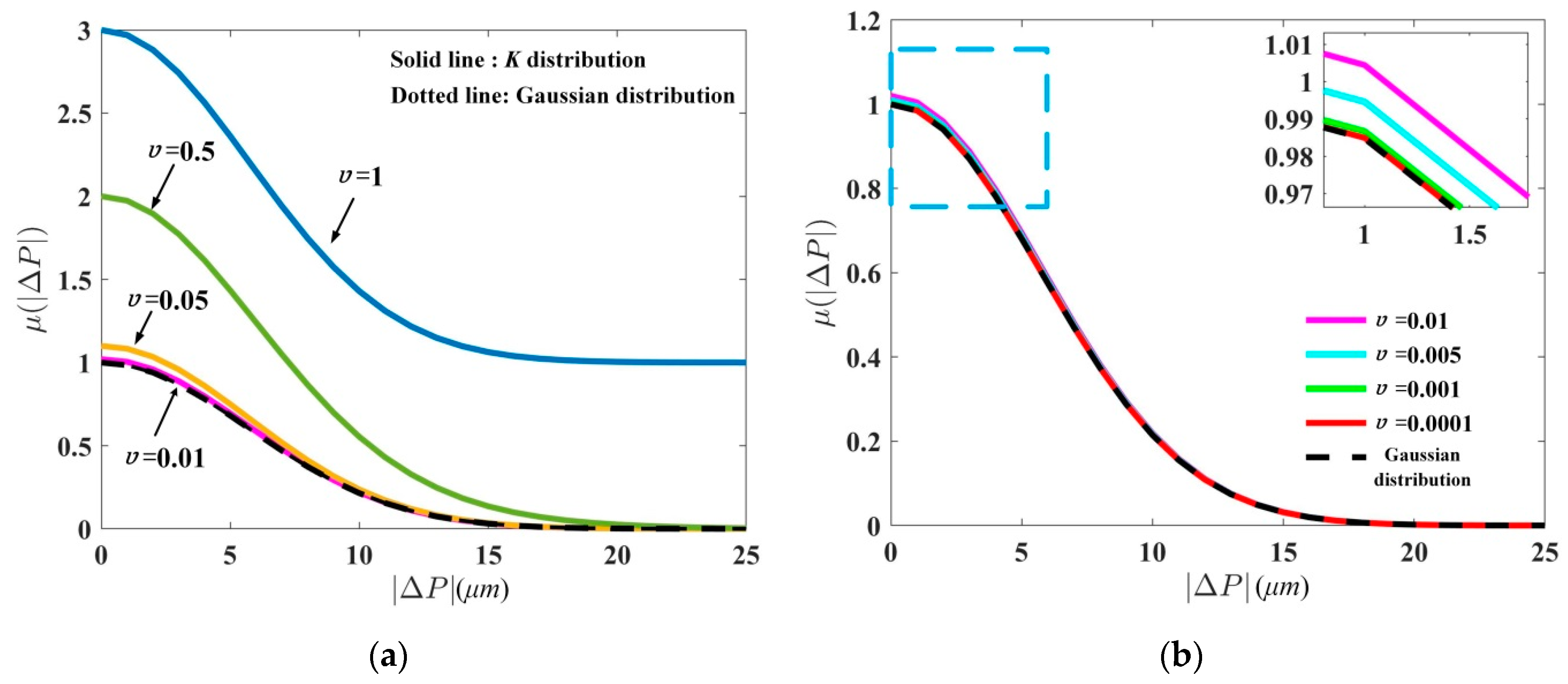
2.2. Spatial Correlation Property

To analyze the spatial correlation function of double speckle fields, that is, explore the relationship between two speckles in different positions at the same time, setting τ = 0 in Equation (1a) and the normalized spatial correlation function for K-distributed statistics in the doubly scattered system is derived as:
μ K ( | Δ p | ) = ν exp [ ( 1 ν ) Δ p 2 ρ 2 2 ] + ν exp ( Δ p 2 ρ 2 2 ) + exp ( Δ p 2 ρ 2 2 )
where Δ p = p 2 p 1 .
Set the same condition in Equation (8), the normalized spatial correlation function for Gaussian-distributed statistics in the doubly scattered system is obtained by:
μ G ( | Δ p | ) = exp ( Δ p 2 ρ 2 2 )
It is clear that the parameter υ determines the shape of K-distributed speckles. Assuming λ = 633 nm, a0 = 10 mm, do = 150 mm, thus ρ2 = 3.02 μm. According to Equations (10) and (11), the relationship of spatial correlation function μ ( | Δ p | ) with the spatial difference | Δ p | is illustrated for various values of the quantity υ , as shown in Figure 2. The solid lines and dotted line represent K speckle and Gaussian speckle cases, respectively. It is shown that the parameter of υ plays an important role for K distribution. The spatial correlation function of K-distributed speckles is gradually close to that of Gaussian-distributed speckles with the decrease of the quantity υ , as seen in Figure 2a. The K-distributed statistics can be replaced with the Gaussian statistics when υ is less than or equal 0.01, as shown in Figure 2b.

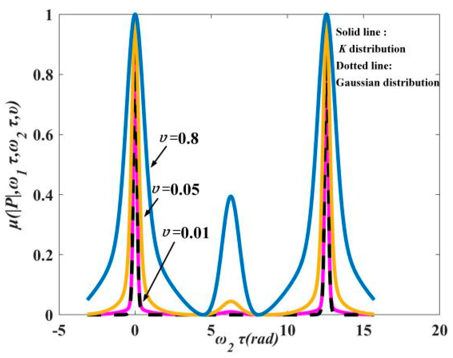
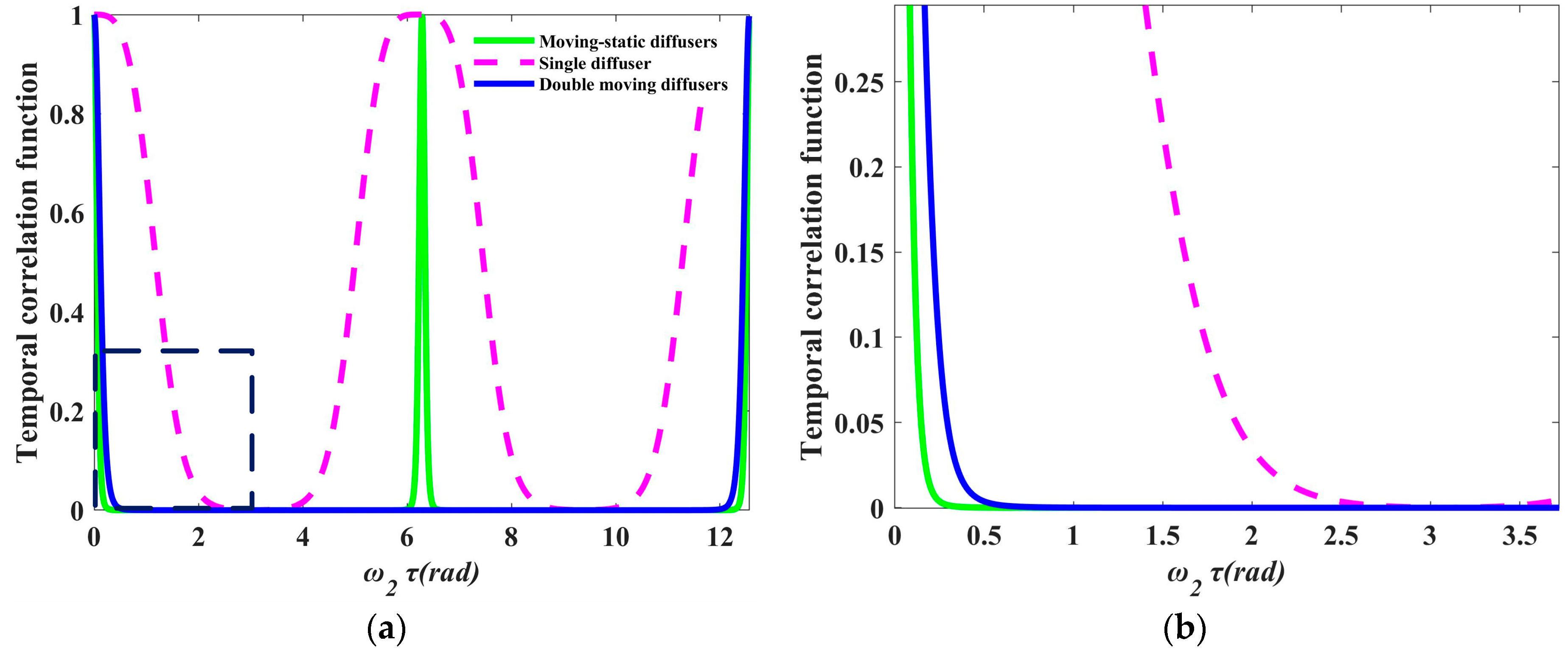
2.3. Temporal Correlation Property

The temporal correlation of double speckle fields is to analyze the speckles relationship in the same position at different time. Setting p1 = p2 = p in Equation (1a), the normalized temporal correlation function for K-distributed statistics in the doubly scattered system is expressed as:
μ K ( | P | , ω 1 τ , ω 2 τ , υ ) = I ( p ) I ( p ) Γ 0 Γ 0 = υ exp [ 2 ( 1 υ ) p 2 ( 1 cos ω 1 τ ) ρ 2 2 ] + υ exp [ 2 p 2 ( 1 cos ω 2 τ ) ρ 2 2 ] + 4 υ 2 [ 1 + υ ( 1 υ ) cos ( ω 1 τ ω 2 τ ) ] 2 × exp { 4 υ 2 p 2 ( 1 cos ω 2 τ ) ρ 2 2 [ 1 + υ ( 1 υ ) cos ( ω 1 τ ω 2 τ ) ] } × exp { 4 ( 1 υ ) p 2 [ 1 cos ( ω 1 τ ω 2 τ ) ] ρ 2 2 [ 1 + υ ( 1 υ ) cos ( ω 1 τ ω 2 τ ) ] }
The normalized temporal correlation function for Gaussian-distributed statistics in the doubly scattered system is obtained from Equation (8) by:
μ G ( | p | , ω 1 τ , ω 2 τ , υ ) = Γ 12 ( | p | , ω 1 τ , ω 2 τ , υ ) Γ 0 = 4 υ 2 [ 1 + υ ( 1 υ ) cos ( ω 1 τ ω 2 τ ) ] 2 × exp { 2 υ ( p p cos ω 2 τ + p sin ω 2 τ ) 2 ρ 2 2 [ 1 + υ ( 1 υ ) cos ( ω 1 τ ω 2 τ ) ] } × exp { 4 p 2 ( 1 υ ) [ 1 cos ( ω 1 τ ω 2 τ ) ] ρ 2 2 [ 1 + υ ( 1 υ ) cos ( ω 1 τ ω 2 τ ) ] }
It is shown that the temporal correlation function is related to the angular velocities of double diffusers except parameter υ . Based on the typical values in Figure 2, the rotating velocity relationship of double diffusers is set as ω1τ = 0.5ω2τ, ω1 ≠ 0, ω2 ≠ 0. According to Equations (12) and (13), the relationship of temporal correlation function with the value of ω2τ is plotted for various values of the quantity υ , as shown in Figure 3. The solid lines and dotted line represent K speckle and Gaussian speckle cases, respectively. It is seen that the curves of K-distributed speckles and Gaussian-distributed speckles nearly coincide when υ is less than or equal 0.01, which corresponds with the conclusion draw from the spatial correlation function.
In a word, the K-distributed statistics can be replaced with the Gaussian statistics when υ is less than or equal 0.01 by spatial correlation property and temporal correlation property, respectively. The Gaussian distribution is adopted because it has advantages such as faster decorrelation rate and lower space–time correlation property. When υ is 0.01, N is calculated as 99, which will provide a reference for the diffuser selection in the experiment. Only selecting diffusers with suitable speckle numbers, the double speckle fields obey the Gaussian distribution with better performance in speckle suppression. Therefore, the comparison of speckle suppression is all performed among single diffuser, static-moving double diffusers, double-moving diffusers in the condition of υ = 0.01.
The work mode of double diffusers with static and moving states is considered with respect to two-moving diffusers, because their speckle reduction results are different. Setting ω2 = 0, and the normalized temporal correlation function for static and moving speckles is given as [18]:
μ ( | p | , ω 1 τ , 0 , υ ) = I ( p ) I ( p ) Γ 0 Γ 2 Γ 0 + Γ 2 = υ 1 + υ exp [ 2 ( 1 υ ) p 2 1 cos ω 1 τ ρ 2 2 ] + 4 υ 2 1 + υ exp [ 4 ( 1 υ ) p 2 1 cos ω 1 τ ρ 2 2 [ 1 + υ ( 1 υ ) cos ω 1 τ ] ] [ 1 + υ ( 1 υ ) cos ω 1 τ ] 2
It is proved that the speckles temporally obey Gaussian statistics in double diffusers with static and moving states regardless of the value of υ .
According to Equations (9), (13) and (14), the temporal correlation functions are plotted in three different diffusers cases when υ = 0.01, as shown in Figure 4. It is clear that the doubly scattered speckles decorrelate faster than the singly scattered speckles. This is related to adding a second diffuser and the control parameter of υ in double moving diffusers case. Furthermore, the period of the correlation function is used for comparison. For the single diffuser and static-moving double diffusers cases, the function period is still 2π. Nevertheless, the period is enlarged to 4π for double-moving diffusers case, which is determined by the diffuser with slower rotational speed. The speckle patterns produced outside the period are replicas of those in the period, which do not improve the speckle suppression result in the averaging process. Therefore, the two moving diffusers configuration can obtain more independent speckle patterns compared with the single diffuser and moving-static double diffusers cases, due to the faster decorrelation rate and larger function period.

3. Experiments

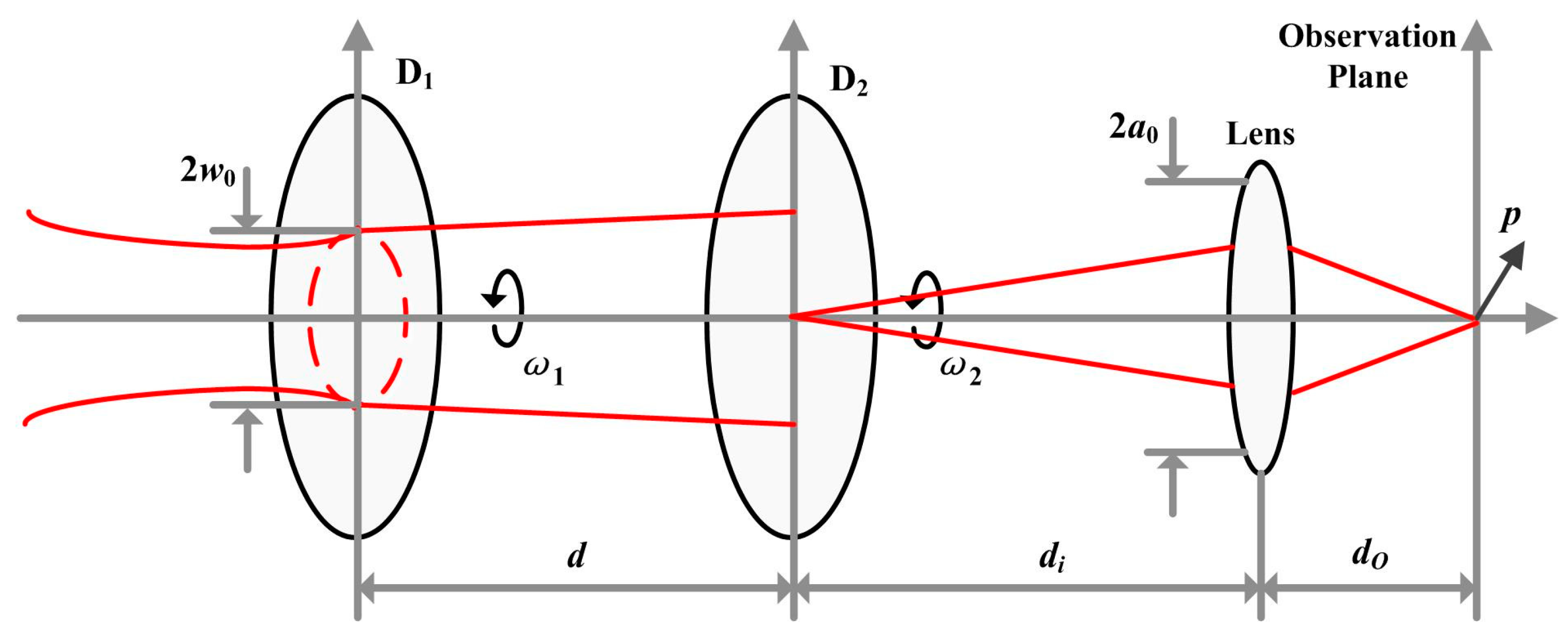
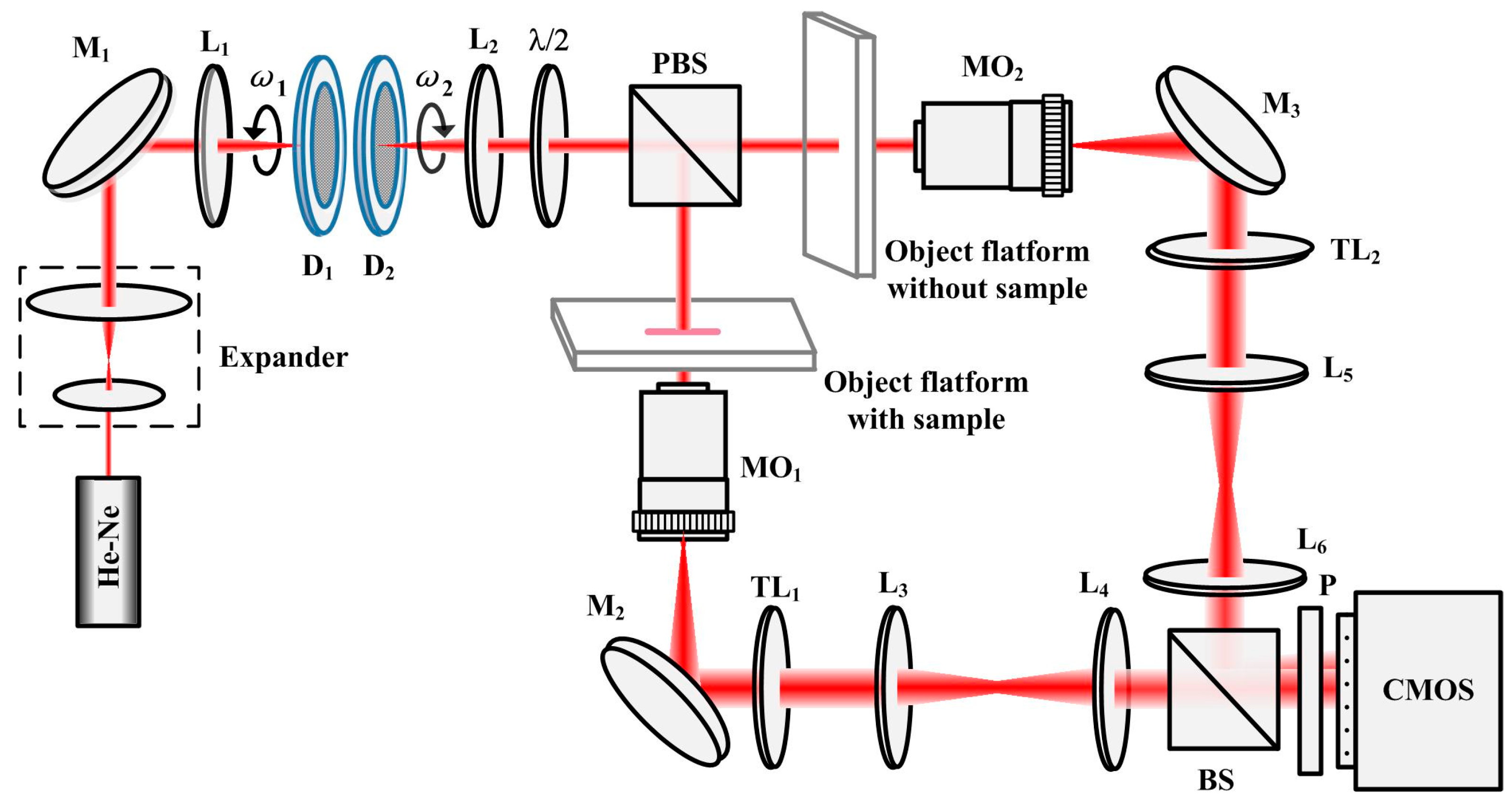
3.1. Experimental Setup

The experimental setup is an off-axis Mach-Zehnder interferometric microscope configuration using two moving diffusers as the dynamic speckle illumination, as shown in Figure 5. A He-Ne laser source illuminates the double rotating diffusers through the expander and L1. The diffusers are mounted in dc motors to realize the automatic rotation, generating the dynamic speckle fields. The linear-polarized laser is split two orthogonal-polarized beams by a polarization beam splitter (PBS), which enter the reference branch and the object branch, respectively. The object beam and the reference beam go through the same optical elements in each branch due to the shorter coherent length, in which the two matching microscopic objectives (MO) are the magnification of 20 and numerical aperture of 0.45. In order to carefully match, the object platforms are placed with and without sample in object arm and reference arm, respectively. The half-wave plate is used to adjust the intensity of two arms. The two beams combine in the beam splitter (BS) and the produced hologram is captured by CMOS. The dynamic speckle field illumination enables to reduce the coherent length of laser source, effectively suppressing the speckle noise.

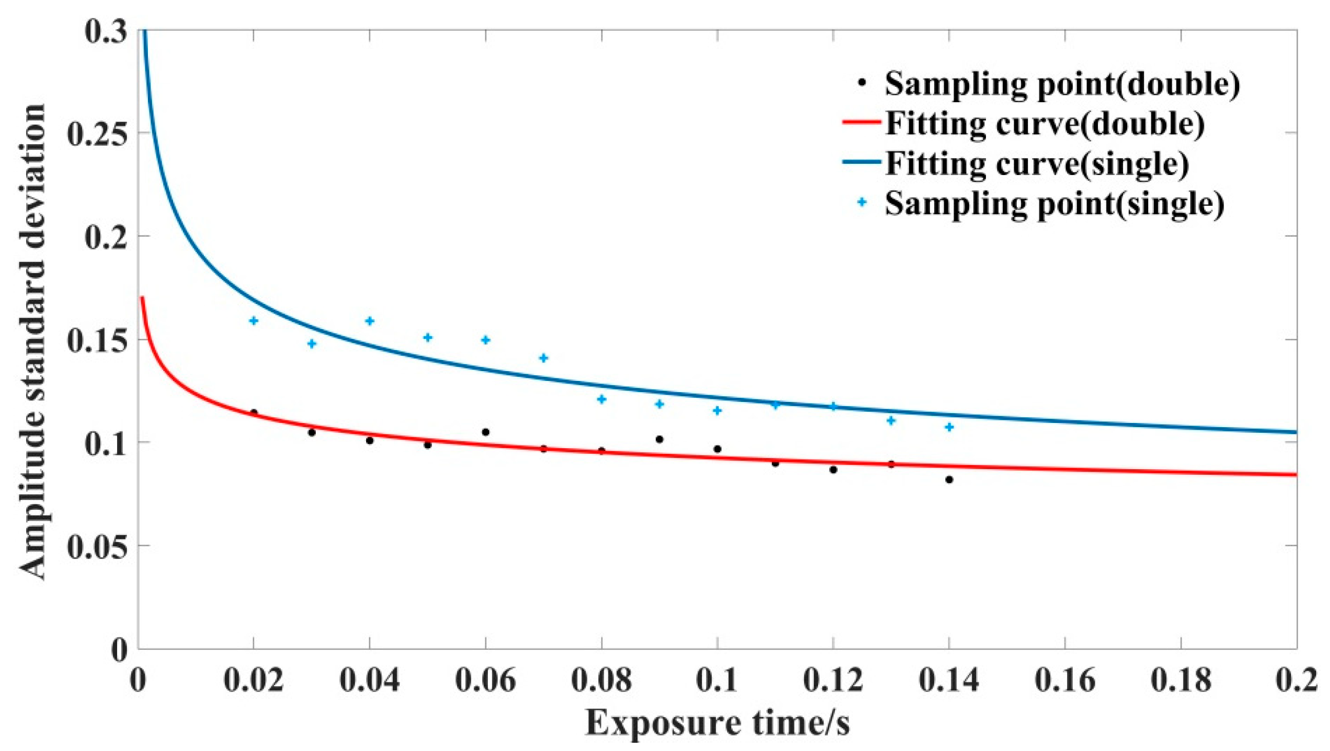
3.2. Comparison of Speckle Suppression Results for Single Diffuser and Double Diffusers

The experiment uses two diffusers with grit 1500, diameter 2 inch and thickness 2 mm to generate the dynamic speckle fields, in which 1500 grit means speckle grain number. In the condition, the speckle fields produced by double diffusers obey the Gaussian distribution. When two diffusers, mounted in two dc motors, are rotated at certain velocity, the region of the sample experiences random walk of time varying field amplitudes and phases. Thus, the speckle intensity on the image plane varies with time. A large number of speckle patterns are averaged out in the camera exposure time, resulting in the coherent noise suppression.
As an example, a transparent step is selected as the experimental specimen. The experiments are performed in two cases, that is, a single rotating diffuser and two rotating diffuses. The typical rotational speed of the diffuser is about 600 rpm. A series of sampled holograms are captured at various exposure times, respectively. Furthermore, the corresponding amplitudes and phases of the step are obtained by the numerical reconstruction algorithm. To make a better comparison, a uniform rectangle region of step is chosen to estimate the speckle suppression performance. The parameter of the reconstructed amplitude standard deviation (SD) is introduced, i.e.,
σ = m = 1 M n = 1 N ( x m , n x ¯ ) 2 M × N 1
where x represents the amplitude distribution, x ¯ is its mean value, and M and N are the pixel number of row and column of the selected region, respectively. With the exposure time variation from 0 to 0.2 s, each reconstructed amplitude SD is calculated for single diffuser and double diffusers cases. Their data and fitted curves are shown in Figure 6. It is shown that the fitted curves of amplitude SD decrease gradually as the exposure time increases. The amplitude SD obtained in two rotating diffusers case is smaller than that in single rotating diffuser obviously. Their amplitude SD is averagely reduced by 25% at the same exposure time. It is demonstrated that the single shot interferogram, by adding a second diffuser, can achieve the better speckle suppression effect in decorrelation rate and independent speckle patterns, which accords with the theoretical analyses and simulation results.

3.3. Comparison of Speckle Suppression Results for Various Diffuser Grits in Doubly Scattered System

It is demonstrated that the smaller υ is, the larger N is in Section 2. The K distribution is closer to Gaussian distribution with N increase for double speckle fields. When the value of N is larger than 99, the speckle fields is viewed as the Gaussian distribution. However, various N, that is various diffuser grits, also affect the speckle suppression results in the Gaussian-distributed filed. The comparison curves of reconstructed amplitude SD for 600 grit and 1500 grit diffusers are presented in doubly scattered system, as shown in Figure 7. The two diffusers rotate at 600 rpm. It is seen that the SD fitting curves possess the downward trends with respect to exposure time change from 0 to 0.2 s. The speckle suppression for double diffusers with 1500 grit is better than that for double diffusers with 600 grit. This is attributed to more different speckle patterns of 1500 grit diffusers in an exposer time.

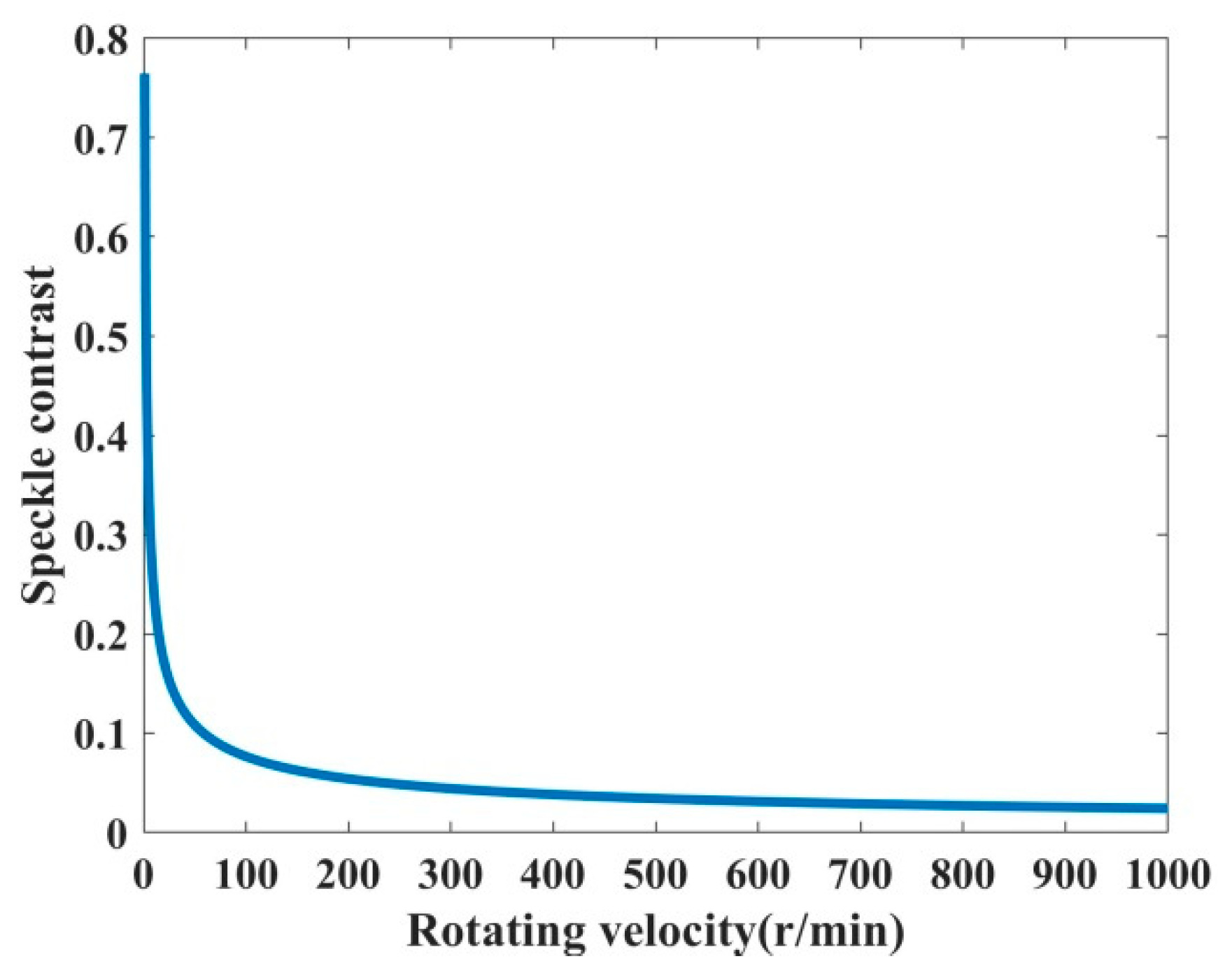
3.4. Comparison of Speckle Suppression Results for Various Rotational Speeds in Doubly Scattered System

Apart from the influence of diffuser grit number, the rotational speed of double diffusers is also related to the speckle suppression. The faster rotational speed is, the shorter corresponding exposure time is. When the hologram is captured in an exposure time, the more independent speckle patterns can be averaged with respect to faster rotational speed, which results in better performance in speckle suppression. The comparison of reconstructed amplitude SD is carried out for 1500 grit diffusers at 300 rpm and 600 rpm in doubly scattered system as shown on Figure 8. The two fitting curves decrease with the increase of exposure time. If the exposure time exceeds a period, the speckle patterns are only replicas of those in the period, which cannot reduce the speckle noise. It is obvious that the speckle suppression result for 1500 grit diffusers at 600 rpm is better than that for 1500 grit diffusers at 300 rpm. Therefore, the rotational speed of 600 rpm and the exposure time of 0.1s are adopted as the experimental condition.
In conclusion, the experiment is performed for 1500 grit diffusers at 600 rpm in doubly scattered system. The hologram captured in exposure time of 0.1 s experiences frequency filtering and numerical reconstruction. The step phase reconstructed is depicted in Figure 9. The 3D phase profile is distributed in the range of 200 × 200 pixels, as shown in Figure 9a. The phase is extracted along the central line of the step in Figure 9b. The 2D profile is displayed in Figure 9c correspondingly. It is seen that the surface fluctuation of the phase is small, and the profile of step is estimated as 5.5 rad.

4. Discussion

In order to realize dynamic measurement, the speckle suppression is carried out only by a single-shot camera capture. Thus, this method of manual rotating diffuser is unavailable. The experiment utilizes two diffusers mounted in the motors to complete automatic rotation. If the sufficiently independent speckle patterns are obtained in an exposure time, the speckles can be reduced after temporal averaging. However, the motors generate vibrations in the motion. The speckle appears in the different patterns accordingly. However, this does not affect the speckle suppression results because the speckle reduction is the averaging process for different speckle patterns. The speckle grain number of diffusers is more, and the speckle patterns may be different when the diffuser vibrates slightly. Furthermore, if the vibrations are large, they will bring unnecessary noise to the image quality. The diffuser requires the suitable rotational speed to reduce vibrations caused by motors. The relationship between the speckle contrast and the rotational speed of diffuser is analyzed. The speckle contrast is related to the speckle intensity, as [20]:
C 80 λ z π 3 f 0 r D T
where z represents the distance between the diffuser and the pupil, f0 is the rotational velocity, r is the radius of diffuser, D is the pupil diameter, and T is the exposure time. Assuming r = 25.4 mm, D = 10 mm, z = 10 mm, T = 0.1 s, thus the speckle contrast result is as shown in Figure 10. It is shown that the speckle contrast gradually reduces with respect to the increase of rotational velocity. When the rotational velocity is larger than 600 rpm, the reduction trend of speckle contrast slows down. In the experiment, the rotating speed of 600 rpm, therefore, it not only reduces the speckle contrast, but decreases the vibrations influence produced by motors.

5. Conclusions

A dynamic speckle illumination method by rotating double diffusers is presented in digital holographic microscopy. The double diffusers, mounted in two dc motors, rotate at certain velocity to generate the large number of decorrelation speckle patterns. They are averaged out in single-shot exposure time, resulting in the coherent noise reduction. From the spatial correlation function and the temporal correlation function, the theoretical analyses and simulations are performed for double speckle fields, respectively. The K-distributed speckles and Gaussian-distributed speckles nearly coincide when υ is less than or equal 0.01, in which the Gaussian distribution has faster decorrelation rate and lower space–time correlation property. When the statistics property obeys the Gaussian distribution, it is demonstrated that the double-moving diffusers configuration can obtain more independent speckle patterns compared with the single diffuser and moving-static double diffusers cases, due to the faster decorrelation rate and the larger function period. The experiments are carried out in single diffuser and double diffusers, various diffuser grits, and various rotational speeds, respectively. The experimental results verify the double-moving diffusers system has better performance in speckle suppression for diffusers with more grit number at faster rotational speed. The approach realizes the reduction in coherent noise only by the single-shot camera capture. This may be applied in the dynamic process records of behavior, growth, and destruction for biological cells.

Author Contributions

Theoretical analysis, Y.L. (Yun Liu) and Y.L. (Yumeng Liu); methodology, M.J.; software, X.W.; validation, P.B. and J.X.; formal analysis, T.L.; writing—original draft preparation, Y.L. (Yun Liu); writing—review and editing, Y.L. (Yun Liu) and K.K. All authors have read and agreed to the published version of the manuscript.

Funding

This research was funded by National Natural Science Foundation of China (Grant No. 61805195, 51875455, 61803302, 61805196), Natural Science Basic Research Plan in Shaanxi Province of China (Grant No. 2019JM-095, 2020JM-465), Key Laboratory Project of Education Department of Shaanxi Province (Grant No. 18JS069), Xi’an Science and Technology Plan Project (Grant No. 2020KJRC0079), Scientific Research Plan Projects of Shaanxi Education Department (Grant No. 20JK0810) and China Postdoctoral Science Foundation (Grant No. 2020M683683XB).

Institutional Review Board Statement

Not applicable.

Informed Consent Statement

Not applicable.

Data Availability Statement

Not applicable.

Conflicts of Interest

The authors declare no conflict of interest.

References

  1. Park, H.J.; Lee, S.Y.; Ji, M.; Kim, K.; Son, Y.H.; Jang, S.; Park, Y.K. Measuring cell surface area and deformability of individual human red blood cells over blood storage using quantitative phase imaging. Sci. Rep. 2016, 6, 34257. [Google Scholar] [CrossRef] [PubMed] [Green Version]
  2. Cao, R.; Xiao, W.; Wu, X.; Sun, L.; Pan, F. Quantitative observations on cytoskeleton changes of osteocytes at different cell parts using digital holographic microscopy. Biomed. Opt. Express 2018, 9, 72–85. [Google Scholar] [CrossRef] [PubMed] [Green Version]
  3. Wittkopp, J.M.; Khoo, T.C.; Carney, S.; Kai, P.; Bahreini, S.J.; Tubbesing, K.; Mahajan, S.; Sharikova, A.; Petruccelli, J.C.; Khmaladze, A. Comparative phase imaging of live cells by digital holographic microscopy and transport of intensity equation methods. Opt. Express 2020, 28, 6123–6133. [Google Scholar] [CrossRef] [PubMed]
  4. Liu, Y.; Zhao, W.; Huang, J.H. Recent progress on aberration compensation and coherent noise suppression in digital holography. Appl. Sci. 2018, 8, 444. [Google Scholar] [CrossRef] [Green Version]
  5. Quan, C.; Tay, C.J. Speckle noise reduction in digital holography by multiple holograms. Opt. Eng. 2007, 46, 115801. [Google Scholar]
  6. Dong, J.; Jia, S.H.; Yu, H.Q. Hybrid method for speckle noise reduction in digital holography. J. Opt. Soc. Am. A 2019, 36, D14–D22. [Google Scholar] [CrossRef] [PubMed]
  7. Nomura, T.; Okamura, M.; Nitanai, E.; Numata, T. Image quality improvement of digital holography by superposition of reconstructed images obtained by multiple wavelengths. Appl. Opt. 2008, 47, 38–43. [Google Scholar] [CrossRef] [PubMed]
  8. Rong, L.; Xiao, W.; Pan, F.; Liu, S.; Li, R. Speckle noise reduction in digital holography by use of multiple polarization holograms. Chin. Opt. Lett. 2010, 8, 653–655. [Google Scholar] [CrossRef]
  9. Xiao, W.; Zhang, J.; Rong, L.; Pan, F.; Liu, S.; Wang, F.J.; He, A.X. Improvement of speckle noise suppression in digital holography by rotating linear polarization state. Chin. Opt. Lett. 2011, 9, 36–38. [Google Scholar]
  10. Pan, F.; Xiao, W.; Liu, S.; Wang, F.J.; Rong, L.; Li, R. Coherent noise reduction in digital holographic phase contrast microscopy by slightly shifting object. Opt. Express 2011, 19, 3862–3869. [Google Scholar] [CrossRef] [PubMed]
  11. Liu, Y.; Wang, Z.; Huang, J.H.; Gao, J.M.; Li, J.S.; Zhang, Y.; Li, X.M. Coherent noise reduction of reconstruction of digital holographic microscopy using a laterally shifting hologram aperture. Opt. Eng. 2016, 55, 121725. [Google Scholar] [CrossRef]
  12. Kubota, S.; Goodman, J.W. Very efficient speckle contrast reduction realized by moving diffuser device. Appl. Opt. 2010, 49, 4385–4391. [Google Scholar] [CrossRef] [PubMed]
  13. Purcell, M.J.; Kumar, M.; Rand, S.C.; Lakshminarayanan, V. Holographic imaging through a scattering medium by diffuser-aided statistical averaging. J. Opt. Soc. Am. A 2016, 33, 1291–1297. [Google Scholar] [CrossRef] [PubMed]
  14. Park, Y.; Choi, W.; Yaqoob, Z.; Dasari, R.; Badizadegan, K.; Feld, M.S. Speckle-field digital holographic microscopy. Opt. Express 2009, 17, 12285–12292. [Google Scholar] [CrossRef] [PubMed]
  15. Choi, Y.; Yang, T.D.; Lee, K.J.; Choi, W. Full-field and single-shot quantitative phase microscopy using dynamic speckle illumination. Opt. Lett. 2011, 36, 2465–2467. [Google Scholar] [CrossRef] [PubMed]
  16. Choi, Y.; Hosseini, P.; Choi, W.; Dasari, R.R.; So, P.T.C.; Yaqoob, Z. Dynamic speckle illumination wide-field reflection phase microscopy. Opt. Lett. 2014, 39, 6062–6065. [Google Scholar] [CrossRef] [PubMed] [Green Version]
  17. Farrokhi, H.; Boonruangkan, J.; Chun, B.J.; Rohith, T.M.; Mishra, A.; Toh, H.T.; Yoon, H.S.; Kim, Y. Speckle reduction in quantitative phase imaging by generating spatially incoherent laser field at electroactive optical diffusers. Opt. Express 2017, 25, 10791–10800. [Google Scholar] [CrossRef] [PubMed]
  18. Li, D.; Kelly, D.P.; Sheridan, J.T. K speckle: Space–time correlation function of doubly scattered light in an imaging system. J. Opt. Soc. Am. A 2013, 30, 969–978. [Google Scholar] [CrossRef] [PubMed]
  19. Li, D.; Kelly, D.P.; Sheridan, J.T. Speckle suppression by doubly scattering systems. Appl. Opt. 2013, 52, 8617–8626. [Google Scholar] [CrossRef] [PubMed]
  20. Xu, J.C.; Liu, Z.C.; Du, Y.W.; Chai, L.Q.; Xu, Q.; Wang, H. Statistical analysis of interferometric imaging system with rotating diffuser. High Power Laser Part. Beams 2011, 23, 702–706. [Google Scholar]
Figure 1. Optical schematic of doubly scattered system.
Photonics 08 00276 g001
Figure 2. Relationship of spatial correlation function μ ( | Δ p | ) with the spatial difference | Δ p | for various values of υ . (a) 0.01 < υ < 1; (b) υ 0.01 .
Photonics 08 00276 g002
Figure 3. Relationship of temporal correlation function with the value of ω2τ for various values of υ .
Photonics 08 00276 g003
Figure 4. Temporal correlation functions in three different diffusers cases when υ = 0.01 . (a) Temporal correlation function curve; (b) Enlarged region labeled in Figure 4a.
Photonics 08 00276 g004
Figure 5. Experimental setup of doubly scattered system. M: reflector, L and TL: lens, λ/2: half-wave plate, D: diffuser, PBS: polarization beam splitter, MO: microscopic objective, BS: beam splitter, P: polarizer.
Photonics 08 00276 g005
Figure 6. Comparison of fitted curves of amplitude standard deviation in single diffuser and double diffusers cases.
Photonics 08 00276 g006
Figure 7. Comparison of fitted curves of amplitude standard deviation for 600 grit and 1500 grit diffusers in doubly scattered system.
Photonics 08 00276 g007
Figure 8. Comparison of fitted curves of amplitude standard deviation for 1500 grit diffusers at 300 rpm and 600 rpm in doubly scattered system.
Photonics 08 00276 g008
Figure 9. Reconstructed phase of step. (a) 3D profile; (b) Extracting phase along the central line; (c) 2D profile.
Photonics 08 00276 g009
Figure 10. Relationship of speckle contrast with rotational velocity.
Photonics 08 00276 g010
Publisher’s Note: MDPI stays neutral with regard to jurisdictional claims in published maps and institutional affiliations.

