1. Introduction
High-intensity electromagnetic radiation is effectively described via time-dependent classical fields, i.e., using a model without the concept of photons. The reason for the validity of this approximation is related to the number of photons: While, e.g., for fundamental cavity QED experiments, the average photon numbers can be close to unity [
1], a strong laser pulse can correspond to
photons. Clearly, in this case, the absorption or scattering of a few photons is relatively negligible. When the initial laser pulse is considerably attenuated as a consequence of an interaction with matter, the usual rule of thumb also applies for the large number of the ”missing photons” calling again for a classical description.
On the other hand, the intensity of the exciting field can induce strongly nonlinear processes, like the generation of high-order harmonics (HHG) [
2,
3,
4,
5,
6]. This is a phenomenon that is important not only from a fundamental point of view, but also has practical applications, e.g., in the generation of ultrashort pulses [
7]. However, the efficiency of the HHG process is very low, resulting in low photon numbers in the harmonic modes. This implies that the quantum optical description (photon picture) can be relevant for these modes. This picture—once completed—would allow a deeper understanding of the underlying physical processes and eventually lead to more efficient applications.
Considering the quantum optical description of high-field processes, the first fully-quantized, non-perturbative treatment of HHG in the nonlinear Compton process has been given in [
8]. Nonrelativistic description of a charged particle interacting with a quantized mode was also discussed in the early 1980s [
9]. Quantum mechanical transitions between quantized Volkov states were shown to lead to HHG in atoms [
10,
11]. More recently, an interesting relation between the photon number distribution of a laser pulse after the interaction with matter and the HH spectrum has been pointed out in [
12]. Fingerprints of the HH process in the statistics of the ”missing photons” have already been identified using both gaseous [
13] and solid state targets [
14]. Reference [
15] introduces the concept of measurement (post-selection) and claims that the process of HHG changes the initially coherent state of the exciting field into a Schrödinger-cat-type state. In Reference [
16], a general perturbative approach was presented.
Realistic theoretical models should reproduce the well-established experimental findings, such as the qualitative properties of the HHG spectra, which means the appearance of well-defined peaks at integer multiples of the central frequency of the excitation. The heights of these peaks decrease suddenly with increasing frequency (HH order), then a plateau region with comparable peak heights follows, and finally, an intensity-dependent cutoff (when the HH peaks vanish) is observed. Besides this elementary requirement, there are also numerous interesting questions a theoretical model can answer. These include (in increasing order of difficulty to answer):
Photon statistics of the HHG modes: photon number expectation values and higher momenta as well. This allows the characterization of the modes, the determination of their bunching/antibunching properties and possible nonclassicality.
Back-action of the HHG process on the photon statistics of the exciting mode(s). This would allow investigating the statistics of the HHG-related ”missing” photons.
Photon number cross-correlations between different HH modes.
Entanglement between different HH modes. At the time being, there is no experimental evidence for the existence of such strong, purely quantum mechanical correlations. However, since entanglement can be a potential resource for state preparation, it is important to clarify this question.
Possible quantum mechanical entanglement between the state of the material system, the HH modes and the exciting mode(s) have similar relevance.
Correlations between different emitters in a multiatomic sample; propagation effects on the quantized level.
Clearly, knowing the time evolution of the complete system, all these questions can be answered. However, the related numerical problem is computationally very expensive. First of all, short, few-cycle pulses (e.g., with a duration in the femtosecond domain) mean wideband excitation and would require a large number of modes to be taken into account. Additionally, the dimension of the underlying Hilbert space is prohibitively large. Working in photon number eigenbasis, and truncating it for each HH mode, e.g., at 10 photons, we can realistically have a HH Hilbert space with a dimension of This emphasizes the role of analytic approaches, sophisticated numerical methods and physically confirmed approximations in general. Using a simple model for the material system is one of these approximations. In the following, we summarize the results that were obtained using a two-level atom—a concept that is widely used in quantum optics. Obviously, this model cannot account for material-specific effects, but it is particularly useful to see the general, qualitative properties of the HHG process.
The current paper is organized as follows: First, in
Section 2, we introduce the models to be investigated.
Section 3 summarizes the results related to the case of quantized HH modes and classical excitation.
Section 4 discusses the case of a quantized exciting mode, while conclusions are drawn, and an outlook is given in
Section 5.
2. Models
The Hilbert space of the complete, fully quantized problem consists of the tensor product of the Hilbert space describing the material system and the Fock space of the radiation field. For the sake of simplicity, let us use the term ”atom” for the material system. Considering the field, it is not necessary to take all modes into account: frequencies considerably above the cutoff can be safely neglected. The complete Hamiltonian can be written as:
where the first term describes the unperturbed atom, and the Hamiltonian for the free radiation field is formally split into two parts:
describing the excitation and
which corresponds to the HH modes. The light–matter coupling also consists of two terms. Both
and
have the form of
where the sum runs over different modes for the two Hamiltonians. All annihilation operators
commute, and so do all creation operators,
. Additionally,
Considering the material system, in the following, we focus on a two-level atom, for which
where
denotes the appropriate Pauli matrix. The interaction terms have the form of
where
denotes the dipole moment operator, while
is the electric field. In our case, assuming that
is linearly polarized, the relevant component (
for the sake of simplicity) of
can be written as
and
where the summation is over the exciting and HH modes, respectively. Assuming the optical or near infrared domain for the exciting field, the generalized Rabi frequencies
(with
V denoting the quantization volume) are considerably lower than the central frequency of the excitation,
Special samples with particularly large dipole moments (like quantum dots) can be exceptions.
For clarity, let us note that the action of, e.g., the tensor product operator on a state (where denotes an arbitrary atomic state, while is a photon number eigenstate of the ith mode) is given by
It has to be emphasized that the time evolution induced by (
1) is still difficult to calculate, even if we consider the case of a two-level atom. Consequences of further approximations—that include treating certain modes as classical, time-dependent fields, as well as neglecting, e.g., mode-mode correlations—will be analyzed in the following.
3. Classical Excitation, Quantized Harmonics
Since average photon numbers are orders of magnitude lower in the HH modes than in the exciting ones, as a first approach, it is reasonable to consider the excitation to be classical. This means omitting
in Equation (
1), and replacing
with
where
The time-dependent external electric field is assumed to have a finite duration:
If and otherwise. Initially ( before the arrival of the pulse), the state of the atom will be its ground state, while the HH modes are unpopulated (vacuum state).
In order to reduce the number of time-dependent variables, it is useful to concentrate on the expectation values of the relevant operators, like photon numbers. For a numerical solution, it is clear that we can take only a finite number
N of modes into account. Practically,
N can be around a few thousand. The corresponding frequencies do not need to be integer multiples of the central frequency of the excitation, they can be uniformly distributed between zero and the cutoff frequency. Clearly, using a finite number of modes leads to oscillatory dynamics, even without the laser pulse. For reliable results, we have to restrict the calculation to a time interval that is short compared to these (unphysical) oscillations. According to our experience, a frequency spacing of
together with the realistic assumption of
satisfy this requirement for the time scale of the HHG process (around 100 fs), which is determined by
the duration of the exciting pulse, see Equation (
5).
In spite of taking a finite number of modes into account, the set of Heisenberg picture dynamical equations for the relevant operators is infinite: the time derivative of a single operator contains products of two operators, the time derivative of two-operator products contains products of three operators, and so on. Clearly, the same holds for the expectation values as well. In order to obtain a closed set of a finite number of equations, we have to truncate this hierarchy. By taking a look at the interaction Hamiltonian, we see that there is no direct mode–mode interaction. Therefore, we can assume that different HH modes influence the dynamics of each other weakly. This assumption can be checked numerically: taking only two or a single mode into account leads to solvable models. According to our calculations, indeed, the results are numerically equivalent in the two cases.
This allows for a physically justified, consistent truncation of the infinite hierarchy of equations. In detail, let us consider the expectation value
as an example. The weakness of the mode–mode correlations implies that this expectation value is negligible unless
If we apply this rule for all atomic operators
and
and also neglect terms that correspond to two-photon processes (e.g.,
or
), we obtain a closed set of equations. The single-particle expectation values that appear in these equations are
and
Note that
and
W are the components of the Bloch-vector, which allows the visualization of the atomic state on a sphere with a unit radius. The component
W—also called inversion—has the most transparent interpretation,
means that the atom is in its excited state (”north pole” of the Bloch-sphere), while
corresponds to a ground state atom (and the ”south pole” of the Bloch-sphere).
is the photon number expectation value in the
nth mode. The terms
and
which are expectation values of light–matter interaction, also have to be included in order to obtain a closed system of dynamical equations. For
N HH modes, this means
ordinary differential equations for
real variables. They are to be solved using the initial conditions
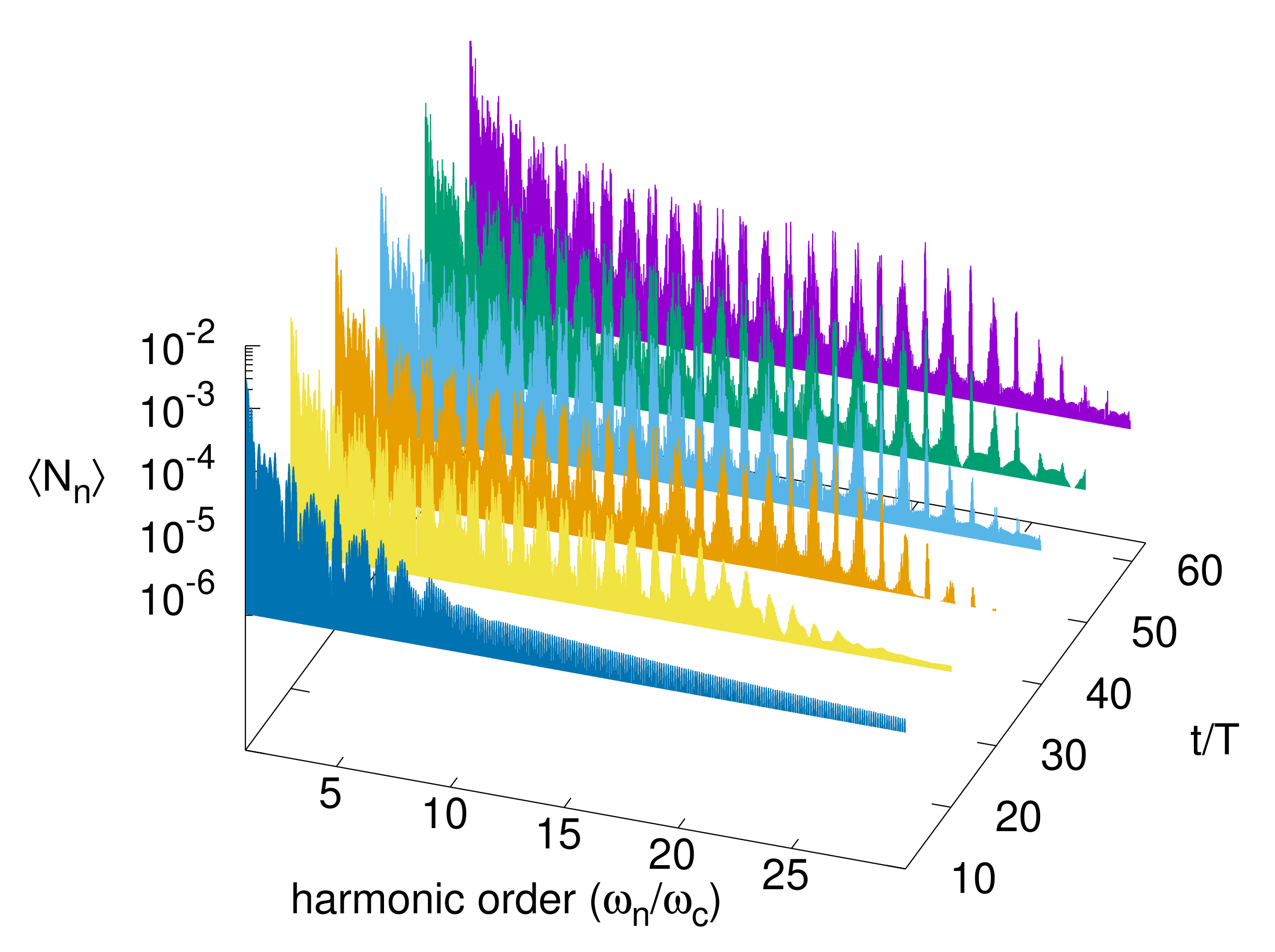
, and all other expectation values are zero. (The atom is in its ground state, and the HH modes are not populated.) Focusing on the photon number expectation values, a typical result can be seen in
Figure 1. The excitation corresponding to this figure is given by Equation (
5), with the central frequency of the exciting field being resonant:
, and we consider many-cycle excitation:
As we can see, the populations of the HH modes build up gradually as the amplitude of the excitation increases. Initially, when the amplitude of the exciting field is considerably lower than its maximal value, modes with lower frequencies become populated. After the maximum of the envelope function, the range of the populated modes practically does not change. When the excitation is over, the photon number expectation values plotted versus the mode frequency resemble experimental HHG power spectra: we can see the well-defined peaks at integer multiples of
a plateau region and also the high-frequency cutoff. The internal structure of the peaks—specifically the observable difference between peaks corresponding to odd and even order harmonics—can be explained, e.g., using a Floquet analysis of the problem [
17]. This is, however, specific to the case of two-level atoms, not expected to be directly applicable to more complex material systems. (For example, for atomic gases—as well as for solids with inversion symmetry—HHG spectra are dominated by odd-order peaks, which is a consequence of the spacetime symmetry of the joint matter-excitation system [
18,
19,
20]. For two-level systems, HH peaks also appear at even multiples of the exciting frequency.)
In order to analyze the photon statistics of the HH modes, the expectation values of the photon numbers are not sufficient, and higher-order momenta are also required. However, if we would like to extend the equations of motion to be able to account for, e.g.,
the number of differential equations to solve (as well as the number of dynamical quantities) would render the numerical solution of the problem practically impossible. However, previous results suggest that the photon statistics of the different modes are almost independent. Therefore we can consider a single mode only, and calculate, e.g., the Mandel parameter
This parameter allows us to compare the width of the photon statistics of the investigated mode to that of coherent states, whose statistics are Poissonian, meaning
In view of this, the case
(
) is considered as super-Poissonian (sub-Poissonian) photon distribution. Clearly, in our case,
is time-dependent. As it is shown in Reference [
17], it exhibits rapid oscillations for all HH modes, and qualitative differences can be found between, e.g., even and odd harmonics. Even the sign of
can change several times, thus it is not completely unambiguous to tell whether these modes have super- or sub-Poissonian statistics during the excitation process.
4. Quantized Excitation, Von-Neumann Lattice and Wigner Functions
Although average photon numbers in the exciting mode(s) can be high, there are experimental results that can only be explained by considering these modes to be quantized [
13,
14]. The process of HHG was shown to affect the photon statistics of the exciting mode in a measurable way: the statistics of the ”missing photons” have a multipeak structure that is very similar to the HHG spectra.
In order to investigate this effect, the first step can be considering a single, quantized exciting mode that is initially in a coherent state
(Note that the photon number expectation value is
in this case, and ”strong excitation” means a large magnitude of the complex number
) Now, recalling Equation (
1), we have
where the terms are given in
Section 2, but in this case, the sum over
n for the exciting modes reduces to a single term, the frequency of which will be denoted simply by
This Hamiltonian is the same as the one corresponding to the well-known Jaynes–Cummings–Paul model [
21], without rotating-wave approximation (RWA). In spite of its seemingly simple form, the analytic solution of this model is far from being trivial. (However, it can be termed as a quantum integrable system, see Reference [
22].) Additionally, even the numerical solution of the dynamics induced by (
9) offers difficulties for large magnitudes of
This is due to the Poissonian statistics of the coherent states—which are most often used for the description of laser modes. When
is large,
is also large, thus the appropriate expansion
in terms of photon number eigenstates
requires unmanageably many of these basis states. Therefore a less conventional approach is needed, which uses a different basis.
In order to develop a treatable numerical approach, it is important to note that the operator
allows for an analytic diagonalization. Within the framework of the two-level approximation,
above can be considered to describe the interaction of a single mode of the electromagnetic radiation with a free electron. (The electron cannot be bound because of the absence of the atomic Hamiltonian.) This implies that although the dynamics induced by
can be solved analytically, it is not expected that the process of HHG can be explained in this way. Indeed—as we shall see later—no HH radiation is produced without the atomic Hamiltonian. This shows that despite the simplicity of the two-level model, general concepts apply to this case as well. Keeping this in mind, we continue the discussion of the dynamics induced by
which provides a starting point for a very transparent interpretation of the HHG process.
Using the displacement operators with appropriate arguments, the degrees of freedom for the exciting mode and the material system decouple:
where
The equation above means that the dynamics without the Hamiltonian of the atomic system can be obtained analytically. For example, if at
, the state is a tensor product
(where
), at a later time instant
we have
Similarly,
evolves into
The time-dependent parameters of the coherent states here are:
and the prefactors are phases:
Clearly, for an initial atomic state that is a superposition of
and
we obtain the corresponding superposition of the time evolved solutions as well. For example, for the ground state
, we obtain
This allows an interpretation in the phase space of the exciting mode, which is identical to the complex plane. As one can check, the coherent states
have the same periodicity as the excitation (
), and the same holds for the prefactors
Thus, without the Hamiltonian for the atomic system, the time evolution is periodic. (This statement is independent from the initial states.) Therefore, it is sufficient to visualize the right-hand side of Equation (
12), e.g., on the interval
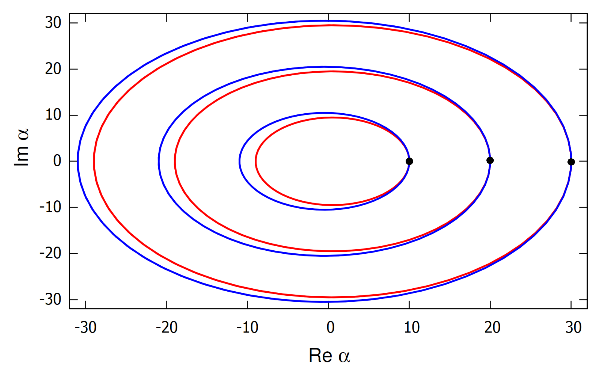
Figure 2 shows the labels
in the case when the initial complex number,
is real. Clearly, at
we have
and the phase-space trajectories that we can associate with the these time-dependent labels are circles. The radii of these circles are different, and their centers are separated by a distance of
see
Figure 2 (this is similar to the results presented in Reference [
15]).
In accord with the discussion following Equation (
10), although the prefactors of the time-dependent coherent states in Equation (
12) contain terms that indicate the appearance of high-order harmonics, no HH emission occurs. In our model, this is related to the fact that the dipole moment operator commutes with
thus its expectation value is a constant of motion. That is—as expected—the atomic Hamiltonian
is also needed for the HH radiation to be emitted. However, in order to see the details of the process, we need an appropriate method to solve the complete dynamics induced by Equation (
9)—at least numerically.
As it was pointed out by J. von Neumann [
23], a discrete subset of coherent states
with
n and
m being integers, forms a (non-orthogonal) basis on the Hilbert-space of a single mode. (The completeness of these states was shown in References [
24,
25].) In Reference [
26], the operator equations for the quantized modes were turned into c-number equations using this basis. It was also demonstrated [
27] that the basis of the von Neumann lattice coherent states turns out to be very useful for calculating how HH radiation emerges on our model.
It can be shown that the complete (infinite) von Neumann lattice is not needed to perform precise numerical calculations [
27]. By choosing a very limited subset of the lattice around the initial coherent state (
points), and rotating it as it is shown by Equation (
12), during the time scale of the HHG process, the action of
will not drive the state of the system outside the subspace spanned by the rotating members of the basis. That is, although the non-orthogonality of the von Neumann lattice states introduces a certain inconvenience, it is a low price to pay for obtaining a small, numerically invariant subspace. Using this approach, quasi-probability distribution functions [
28,
29,
30,
31] can also be calculated in order to describe the quantum state of light in the phase space of the mode [
32].
Instead of using the joint Wigner function for the atom-field system [
33], now it is more instructive to focus on the exciting mode alone. (Technically, in order to obtain the density operator only for the mode, we have to trace over atomic degrees of freedom.) The von Neumann lattice allows an elegant calculation of the Wigner function [
28], which—as it is shown in
Figure 3—leads to transparent interpretation of the HHG process. Considering
as the initial state, during the time evolution, it splits into two parts, as given by Equation (
12). The atomic Hamiltonian
induces transitions between the constituents of the split state (which have different atomic parts). This leads to a rapidly oscillating dipole moment expectation value, which is the source of the HH radiation. Snapshots of the Wigner function that correspond to this time evolution are shown in
Figure 3.
Let us note that for more realistic, pulsed (multimode) excitation, the process we described above—even for several times 10 optical cycles—is much faster than the quantum optical collapse and revival phenomena [
34,
35].
As a generalization, the case of more complex material systems can also be treated using the method discussed above, and the physical interpretation is very similar, too. The expansion of the initial state in the eigenbasis of a general dipole moment operator usually contains more than two terms, which causes the initial state to split into more parts. The atomic Hamiltonian induces transitions between these parts, leading to a time-dependent dipole moment expectation value, and, eventually, high order harmonics.


