Invasive and Non-Invasive Observation of Occluded Fast Transient Events: Computational Tools


Abstract
:1. Introduction
2. Methodology
2.1. Invasive
2.2. Non-Invasive
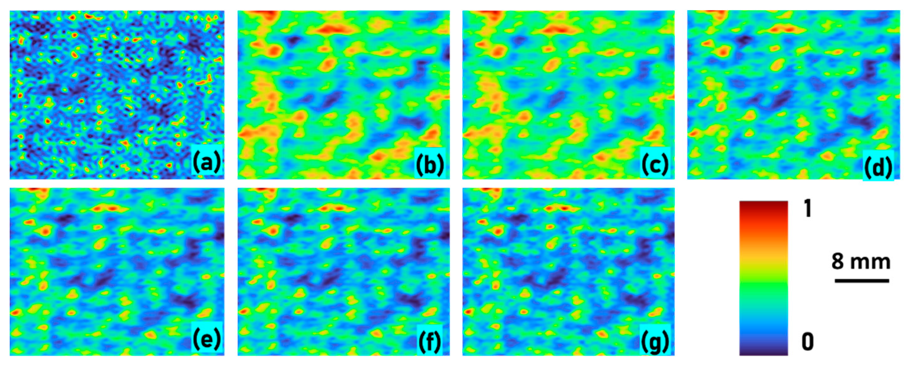
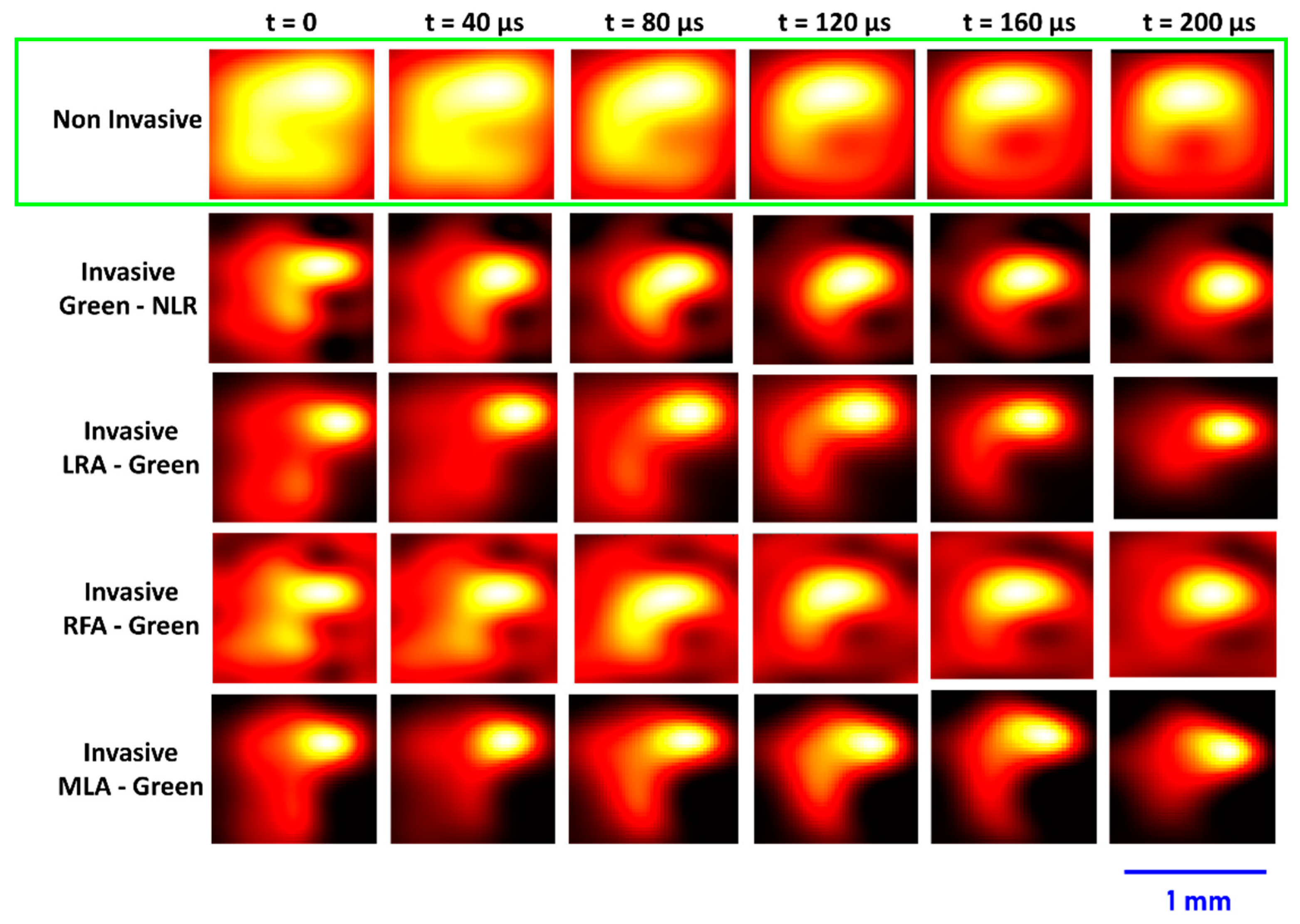
3. Simulative Studies
4. Software
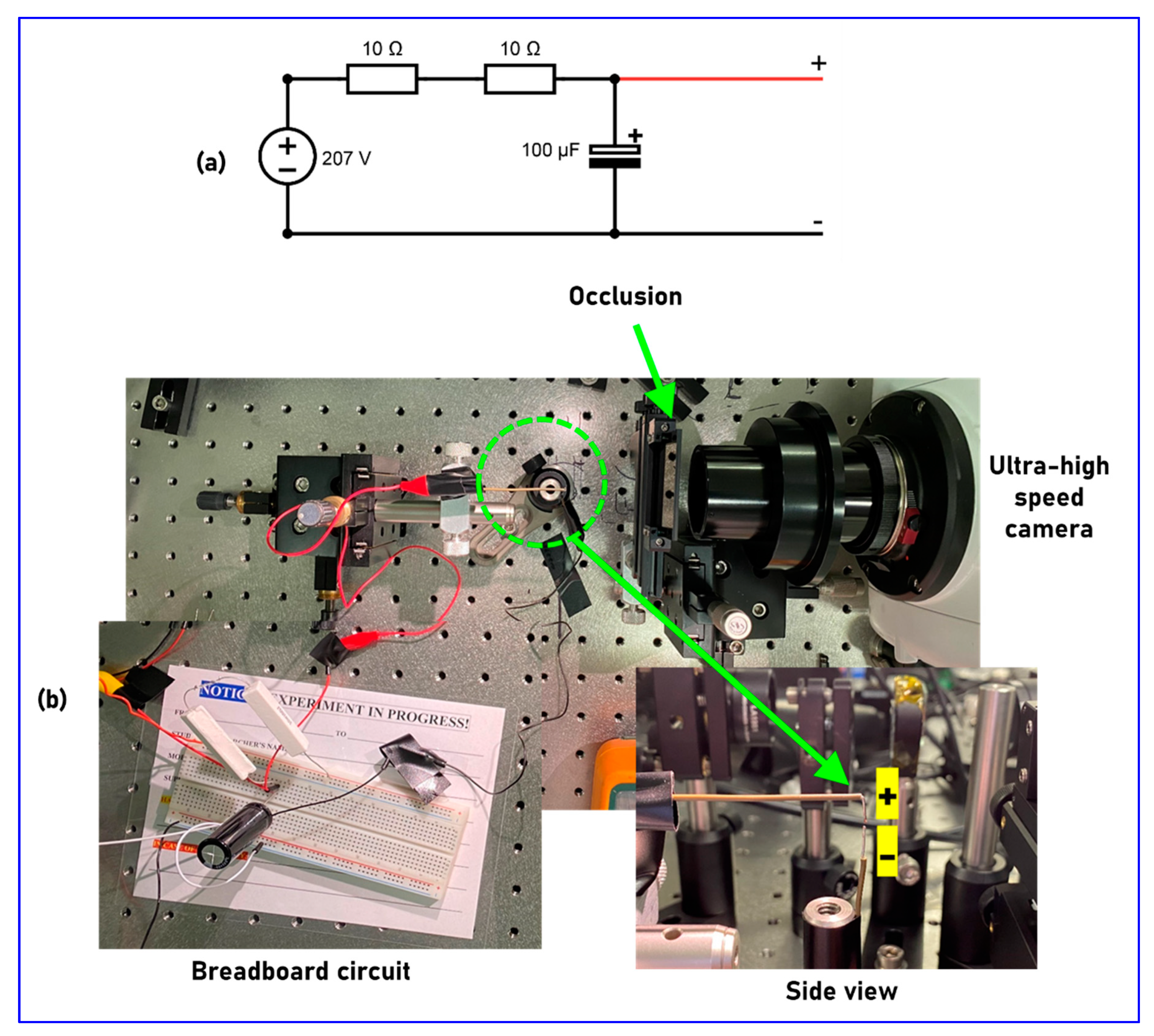
5. Experiments
6. Summary and Conclusions
Supplementary Materials
Author Contributions
Funding
Institutional Review Board Statement
Informed Consent Statement
Data Availability Statement
Acknowledgments
Conflicts of Interest
References
- Fade, J.; Panigrahi, S.; Carré, A.; Frein, L.; Hamel, C.; Bretenaker, F.; Ramachandran, H.; Alouini, M. Long-range polarimetric imaging through fog. Appl. Opt. 2014, 53, 3854–3865. [Google Scholar] [CrossRef] [PubMed] [Green Version]
- Jaruwatanadilok, S.; Ishimaru, A.; Kuga, Y. Optical imaging through clouds and fog. IEEE Trans. Geosci. Remote Sens. 2003, 41, 1834–1843. [Google Scholar] [CrossRef]
- Paciaroni, M.; Linne, M. Single-shot, two-dimensional ballistic imaging through scattering media. Appl. Opt. 2004, 43, 5100–5109. [Google Scholar] [CrossRef]
- Mukherjee, S.; Vijayakumar, A.; Kumar, M.; Rosen, J. 3D imaging through scatterers with interferenceless optical system. Sci. Rep. 2018, 8, 1134. [Google Scholar] [CrossRef] [PubMed]
- Xu, X.; Xie, X.; Thendiyammal, A.; Zhuang, H.; Xie, J.; Liu, Y.; Zhou, J.; Mosk, A.P. Imaging of objects through a thin scattering layer using a spectrally and spatially separated reference. Opt. Express 2018, 26, 15073–15083. [Google Scholar] [CrossRef] [Green Version]
- Katz, O.; Small, E.; Guan, Y.; Silberberg, Y. Noninvasive nonlinear focusing and imaging through strongly scattering turbid layers. Optica 2014, 1, 170–174. [Google Scholar] [CrossRef] [Green Version]
- Anand, V.; Ng, S.H.; Maksimovic, J.; Linklater, D.; Katkus, T.; Ivanova, E.P.; Juodkazis, S. Single shot multispectral multidimensional imaging using chaotic waves. Sci. Rep. 2020, 10, 1–13. [Google Scholar] [CrossRef]
- Vijayakumar, A.; Rosen, J. Spectrum and space resolved 4D imaging by coded aperture correlation holography (COACH) with diffractive objective lens. Opt. Lett. 2017, 42, 947–950. [Google Scholar] [CrossRef]
- Horisaki, R.; Okamoto, Y.; Tanida, J. Single-shot noninvasive three-dimensional imaging through scattering media. Opt. Lett. 2019, 44, 4032–4035. [Google Scholar] [CrossRef] [Green Version]
- Takasaki, K.T.; Fleischer, J.W. Phase-space measurement for depth-resolved memory-effect imaging. Opt. Express 2014, 22, 31426–31433. [Google Scholar] [CrossRef]
- Singh, A.K.; Naik, D.N.; Pedrini, G.; Takeda, M.; Osten, W. Exploiting scattering media for exploring 3D objects. Light Sci. Appl. 2017, 6, e16219. [Google Scholar] [CrossRef]
- Vijayakumar, A.; Kashter, Y.; Kelner, R.; Rosen, J. Coded aperture correlation holography–A new type of incoherent digital holograms. Opt. Express 2016, 24, 12430–12441. [Google Scholar] [CrossRef]
- Horner, J.L.; Gianino, P.D. Phase-only matched filtering. Appl. Opt. 1984, 23, 812–816. [Google Scholar] [CrossRef]
- Rai, M.R.; Vijayakumar, A.; Rosen, J. Non-linear adaptive three-dimensional imaging with interferenceless coded aperture correlation holography (I-COACH). Opt. Express 2018, 26, 18143–18154. [Google Scholar] [CrossRef]
- Hardie, R.C.; Barnard, K.J.; Ordonez, R. Fast super-resolution with affine motion using an adaptive Wiener filter and its application to airborne imaging. Opt. Express 2011, 19, 26208–26231. [Google Scholar] [CrossRef] [Green Version]
- Richardson, W.H. Bayesian-based iterative method of image restoration. J. Opt. Soc. Am. 1972, 62, 55–59. [Google Scholar] [CrossRef]
- Lucy, L.B. An iterative technique for the rectification of observed distributions. Astron. J. 1974, 79, 745–754. [Google Scholar] [CrossRef] [Green Version]
- Biggs, D.S.C.; Andrews, M. Acceleration of iterative image restoration algorithms. Appl. Opt. 1997, 36, 1766–1775. [Google Scholar] [CrossRef] [PubMed] [Green Version]
- Gonzalez, R.C.; Woods, R.E. Digital Image Processing; Addison-Wesley Publishing Company, Inc.: Boston, MA, USA, 1992. [Google Scholar]
- Anand, V.; Katkus, T.; Lundgaard, S.; Linklater, D.P.; Ivanova, E.P.; Ng, S.H.; Juodkazis, S. Fresnel incoherent correlation holography with single camera shot. Opto-Electron. Adv. 2020, 3, 200004. [Google Scholar]
- Bertolotti, J.; van Putten, E.G.; Blum, C.; Lagendijk, A.; Vos, W.L.; Mosk, A.P. Non-invasive imaging through opaque scattering layers. Nature 2012, 491, 232–234. [Google Scholar] [CrossRef]
- Mukherjee, S.; Vijayakumar, A.; Rosen, J. Spatial light modulator aided noninvasive imaging through scattering layers. Sci. Rep. 2019, 9, 17670. [Google Scholar] [CrossRef] [PubMed]
- Goodman, J.W. Introduction to Fourier Optics; Roberts and Company Publishers: Greenwood Village, CO, USA, 2005. [Google Scholar]
- Fienup, J.R. Phase retrieval algorithms: A comparison. Appl. Opt. 1982, 21, 2758–2769. [Google Scholar] [CrossRef] [PubMed] [Green Version]
- Vijayakumar, A.; Ng, S.H.; Katkus, T.; Juodkazis, S. Spatio-spectral-temporal imaging of fast transient phenomena using a random array of pinholes. Adv. Photo Res. 2021, 2, 2000032. [Google Scholar]
- Anand, V.; Rosen, J.; Ng, S.H.; Katkus, T.; Linklater, D.P.; Ivanova, E.P.; Juodkazis, S. Edge and Contrast Enhancement Using Spatially Incoherent Correlation Holography Techniques. Photonics 2021, 8, 224. [Google Scholar] [CrossRef]


| Task. No | Task | Steps |
|---|---|---|
| 1 | Defining computational space | Step-I Define the length and breadth of the computational space in pixels (N1, N2). Step-II Define origin (0, 0), x and y coordinates: x = (1 to N1), y = (1 to N2). Step-III Create meshgrid: (X,Y) = meshgrid (x, y). |
| 2 | Load experimentally recorded object intensity pattern and PSF and carry out low pass filtering | Step-I Read image files of object intensity pattern and PSF and convert them into double precision arrays and choose one of the channels of RGB. Step-II Define radial coordinate using the coordinates of the meshgrid . Calculate Fourier transform of the two processed matrices and and select the radial range of spatial frequencies (For R > r, and ) calculate the inverse Fourier transform, where the prime symbol indicates processed matrices and r is the spatial frequency range. The absolute value of the resulting matrices namely O″ and IPSF″ can be used for further processing. |
| 3 | Reconstruction |
Normalise O″ and IPSF″. Step-I . Step-II for different values of α and β ranging from −1 to 1 in steps of 0.1 and calculate inverse Fourier transform. Calculate entropy and find the optimal reconstruction. α = 1, and β = 1, Matched filter. α = 0, and β = 1, Phase-only filter. α = −1, and β = 1, Weiner or inverse filter. Step-III Apply median filter to the optimal reconstruction. Step-IV Display the result. |
| Task. No | Task | Steps |
|---|---|---|
| 1 | Defining computational space | Step-I Define the length and breadth of the computational space in pixels (N1, N2). Step-II Define origin (0, 0), x and y coordinates: x = (1 to N1), y = (1 to N2). Step-III Create meshgrid: (X, Y) = meshgrid (x, y). |
| 2 | Load experimentally recorded object intensity pattern, carry out low pass filtering and autocorrelation and determine parameters | Step-I Read image files of object intensity pattern, convert it into double precision arrays and choose one of the channels of RGB. Step-II Define radial coordinate using the coordinates of the meshgrid . Calculate Fourier transform of the processed matrix and select the radial range of spatial frequencies (For R > r, ) calculate the inverse Fourier transform, where the prime symbol indicates processed matrices and r is the spatial frequency range. The absolute value of the resulting matrix namely O’’ is extracted, the minimum value was subtracted and normalized again. The magnitude of Fourier transform of the object is calculated as which is used in the phase retrieval algorithm. Step-III Set the size of the object and generate the initial guess object function from the extension of the autocorrelation function and low pass filter. |
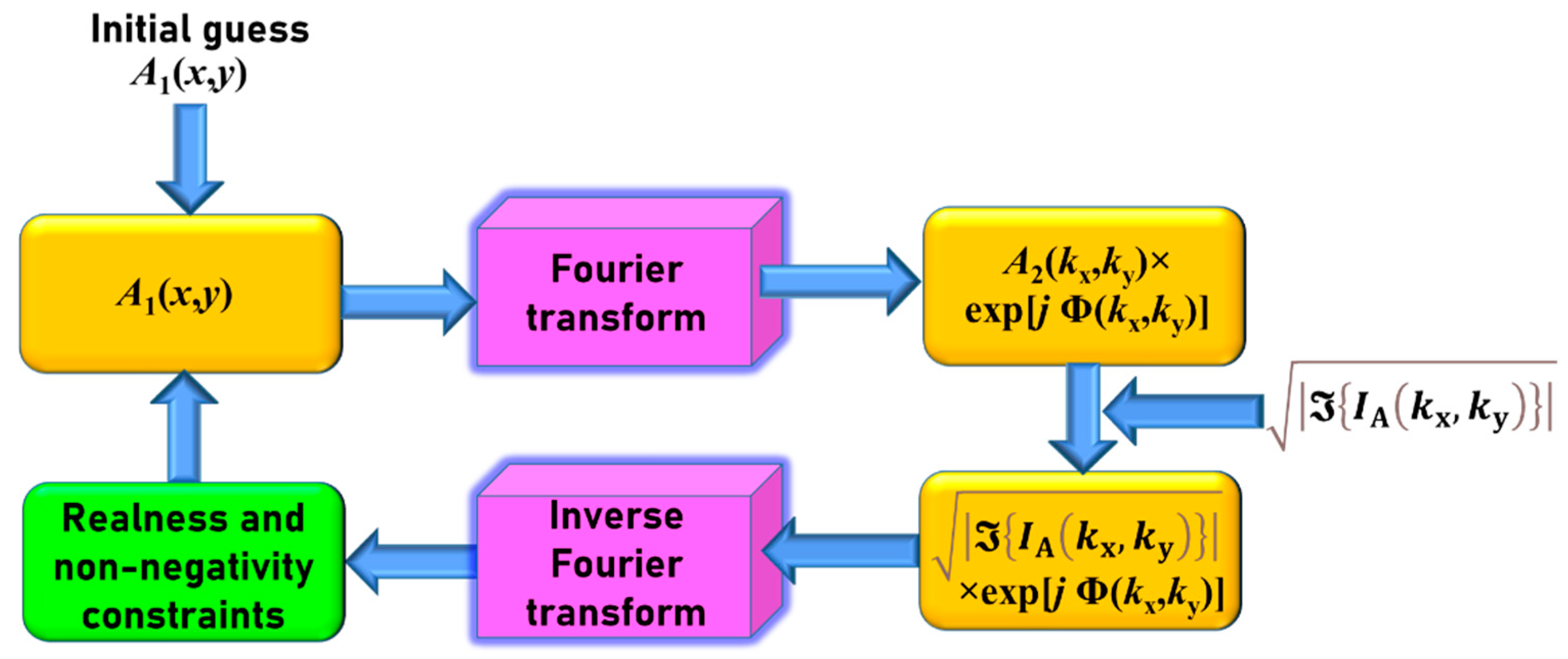
| 3 | Phase retrieval algorithm (Figure 2) | Start for loop Step-I Calculate Fourier transform of the initial guess object matrix A1(x, y) which produces A2(x, y)exp[jΦ(kx, ky)]. Step-II Replace A2(x, y) by and calculate inverse Fourier transform. Step-III Apply constraints—real and object size. End for loop |
Publisher’s Note: MDPI stays neutral with regard to jurisdictional claims in published maps and institutional affiliations. |
© 2021 by the authors. Licensee MDPI, Basel, Switzerland. This article is an open access article distributed under the terms and conditions of the Creative Commons Attribution (CC BY) license (https://creativecommons.org/licenses/by/4.0/).
Share and Cite
Ng, S.H.; Anand, V.; Katkus, T.; Juodkazis, S. Invasive and Non-Invasive Observation of Occluded Fast Transient Events: Computational Tools. Photonics 2021, 8, 253. https://doi.org/10.3390/photonics8070253
Ng SH, Anand V, Katkus T, Juodkazis S. Invasive and Non-Invasive Observation of Occluded Fast Transient Events: Computational Tools. Photonics. 2021; 8(7):253. https://doi.org/10.3390/photonics8070253
Chicago/Turabian StyleNg, Soon Hock, Vijayakumar Anand, Tomas Katkus, and Saulius Juodkazis. 2021. "Invasive and Non-Invasive Observation of Occluded Fast Transient Events: Computational Tools" Photonics 8, no. 7: 253. https://doi.org/10.3390/photonics8070253