Article

New Energy Power System Dynamic Security and Stability Region Calculation Based on AVURPSO-RLS Hybrid Algorithm

1
College of Electrical Engineering, Xinjiang University, Urumqi 830047, China
2
Student Affairs Department, Changsha University of Technology, Changsha 410114, China
3
Nari Technology Co., Ltd., Nanjing 211106, China
*
Authors to whom correspondence should be addressed.
Processes 2023, 11(4), 1269; https://doi.org/10.3390/pr11041269
Submission received: 25 November 2022 / Revised: 3 April 2023 / Accepted: 6 April 2023 / Published: 19 April 2023
(This article belongs to the Special Issue Advances in Electrical Systems and Power Networks)

Abstract

:
Using a high proportion of new energy is becoming the development trend of the modern power industry, with broad application prospects and potential threats to power system operation safety. This paper proposes a hybrid adaptive velocity update relaxation particle swarm optimization algorithm (AVURPSO) and recursive least square (RLS) method to quickly estimate the DSSR boundary using hyper-plane expression. Firstly, the operating point data in the high-dimension nodal injection space are analyzed using the AVURPSO algorithm to identify the key generators, equivalent search space, and critical points, which have relatively great effects on transient angle stability. The hyper-plane expression of the DSSR boundary, which matches the critical points best, is finally fitted by the RLS approach. Hence, the adopted algorithm is applied to rapidly approximate the DSSR boundary by hyper-plane expression in power injection spaces. Finally, the proposed algorithm is validated using a simulation case study on three wind farm regions of the actual Hami Power Grid of China using the DIgSILENT/Power Factory software. Consequently, the mentioned method effectively captures the security stability boundary of the new energy power system and realizes the three-dimensional visualization space of DSSR. By leveraging the DSSR, the state analysis can be conducted rapidly on several parameters, including security and stability assessments in relation to various energy supply capabilities. Meanwhile, these indices are calculated offline and applied online. The findings of this investigation confirm the efficacy and accuracy of the suggested modeling used in the analyzed system, offering technical assistance ensuring the stability of the new energy power system. The DSSR allows the rapid analysis of several parameters, including security and stability assessments with various energy supply capabilities.

1. Introduction

China is seeking to improve the deteriorating natural environment, alleviate the shortage of energy and fuel, build a clean, low-carbon, safe and efficient energy system, implement new energy replacement actions, deepen the reform of the power system, and establish a new power system with new energy as the mainstay [1,2]. China has abundant new energy resources and large storage capacity for economic and environmentally friendly new energy, and can meet the load requirements for the construction and exploration of new energy, propelling it to the forefront [3]. As a clean and pollution-free system, wind energy stands out among clean energy sources [4]. With the increasing proportion of wind turbines being connected to the grid, their high randomness and volatility are also introduced into the grid, thus posing new challenges to the stability and security of the system [5]. To minimize the operation cost of the system and improve operation security, modern power systems use high-voltage transmission lines with large transmission capacities to interconnect regional power grids. These interconnection systems can enhance the transmission efficiency of the system, allowing the better centralization of frequency modulations during fluctuations, and facilitating assistance between interconnected systems [6]. Since regional power grids rely more closely on each other, once a fault occurs in a specific region, its strong connection with other power grids can trigger large-scale cascading failures across interconnected power grids. Consequently, ensuring system security is becoming increasingly important [7]. In addition, the stable operation of the system also impacts the wind generator itself. Voltage that is too low will lead to the low voltage crossing of the wind turbine, while too-high voltage can cause wind turbine faults and even off-grid operation [8]. Thus, analyzing the stability of large-scale new energy power systems is of significant practical importance [9].
The strong uncertainty of wind turbines leads to greater complexity and changeable operation conditions in the power grid, making security analysis of the system more challenging [10]. Moreover, due to the limited scope for the calculation and analysis of the system’s operation status after a large accident, the system cannot meet the requirements of real-time online analysis. Since traditional power system security analysis methods show great limitations and conservatism, it is urgent to develop a new analysis method that can adapt to the current complex power system. The “security domain” method is a novel approach that was developed based on the point-by-point method, which considers the problem from the perspective of the domain and describes the region wherein generally safe and stable operation is possible. The relative relationship between system operation points and the security stability region (SSR) boundary can provide safety margin and optimal control information, leading to the more scientific and effective online real-time safety monitoring, defense, and control of power systems. In 1975, E. Hnyilicza et al. proposed a power system security region analysis method [11,12]. In relation to the overall level of the region, the security domain encompasses the range of boundaries that ensure the overall safe operation of the entire system [13]. The SSR outlines the continuity domain wherein the system can operate safely, which has good adaptability when the system’s operation mode is constantly changing. Moreover, the safety domain method can be used to judge the safety state of the system as a whole—not only can the safety of the operating point be judged according to whether it is in the safety domain or not, but the operator can also obtain the safety margin in each direction and the optimal control direction with reference to the distance of the operating point in high-dimensional space to the boundary of the safety domain, which is important information to decision-making [14].
Therefore, the concept of the security stability region (SSR) is proposed to help develop a new method of power system stability analysis. The primary problem facing the construction of the SSR is the fast identification of the critical point of stable operation, and the forming of the boundary of the SSR [15]. Given the grid structure (topology and component parameters) and the expected fault conditions, the safety domain is uniquely determined in the node injection space, and thus can be calculated offline and applied online. Compared with the traditional “point-by-point” method, the safety domain approach is less computationally intensive and is faster, thus saving time for real-time decision analysis when applied in online safety assessment. Moreover, specific security and stability issues have led to the development of the static security stability region (SSSR), small disturbance security stability region (SD-SSR), and dynamic security stability region (DSSR) concepts. Among these, research on the SSSR in modern power systems has become relatively more mature than that on the latter two. On the contrary, after a given fault, the system remains safe and stable up to a certain power injection point on the injection space, and this operating point is called the stable operating point. The DSSR is the set of all stable operating points [16]. For a given fault, it is only necessary to determine whether its injected power point lies within the DSSR, and the safety margin of the system can be derived according to the relative position of this power point, which is convenient and can be applied online. At the same time, the operators can also develop corresponding control strategies and scheduling plans based on the relative positions of the power injection points, in order to achieve effective online safety evaluations and optimization. Currently, the more mature method for calculating DSR is the fitting method [17]. The fitting method is the most widely used and mature method. The key to this proposed method is to obtain sufficient critical injection points via numerical simulation. Then, the bounding hyperplane is obtained by fitting it with the mathematical analysis method, the least squares method. Although this method has high computational accuracy, the time required to search for critical points is long, especially in relation to the increasingly complex and large-scale interconnected power grids, and the utility of the fitting method is greatly reduced here. On this basis, F. F. Wu proposed the concept of the inscribed hyperplane. The inscribed hyperplane is a subdomain of the DSSR, and the upper and lower constraints of node injection quantity describe its mapping relationship. Reference [18] proved that the boundary of the security region can be represented by a set of one or more hyperplanes in the field of engineering. Ref. [19] carried out a piecewise approximation of the boundary of the SSSR based on the relationship between the space angle of the space tangent vector at the critical point and the maximum space angle threshold. Reference [20] used the Taylor series trajectory sensitivity method to identify the security region. The above study aimed to improve the efficiency and accuracy of security domain construction. However, in the calculation of the DSSR, since the SSR boundary as a hyperplane and the injected power vector as spatial points can be formed, the following obviously holds. (1) When the power operating point is inside the SSR, if the point is further away from the SSR boundary, the system is safer; when the point is closer to the system boundary, it means that the system is closer to the critical state. (2) When the power operation point is outside the SSR, if the point is farther away from the SSR boundary, the system deviates from the steady state; when the point is closer to the system boundary, it means the system is closer to the critical state.
At present, China’s power system is developing rapidly, and the conditions of regional interconnection, HVDC transmission, and north–south mutual supply have led to a more complex structure and increases in the scale of the power grid. In order to evaluate the safety and stability of the system after a fault, and to ensure the economy and safety of transmission and distribution, a transient stability simulation of the system is required. When DSSR is used to analyze the safety of large interconnected grids, a large number of numerical simulations are required. Due to the limitations of simulation conditions and practicality requirements, effective and appropriate DSSR simulations must be performed for large-scale power systems in order to reduce the computational effort and improve the practicality of the algorithm [21,22]. Refs. [23,24] provide a detailed analysis of the DSSR, and propose the following topological properties: (1) there is no “hole” inside the DSSR—as long as the injected power vector is inside the SSR, the system can remain transient and stable under perturbations; (2) there is no “island” outside the DSSR, and no “knot”—if the injected power vector is outside the SSR, it means that the injection will cause transient instability; (3) the boundary of the DSSR can be expressed as a concatenation of multiple directional surfaces, or as a common fit. The above properties provide an important reference for the dynamic full domain to be practically applied, such that in practical applications, as long as the SSR boundary is calculated, the system’s state of stability can be judged by analyzing the relationship between the realistic power injection and the SSR boundary. On this basis, further quantitative analyses can be performed [25,26,27,28].
The fitting method calculates the dynamic safety domain by locating the critical operating points of the system through a large number of simulations of the system notation, and after obtaining a set of critical operating points, this point group is fitted to obtain the dynamic safety domain hyperplane boundary; the fitting method is generally least squares. The fitting method makes full use of the dynamic safety domain properties, is conceptually simple and intuitive, and is robust and easy to apply, while being computationally intensive [29,30]. The specific methods are as follows:
I.
Search for critical points—(1) Given the system topology, we seek the fault occurrence point, fault type, fault clearance time, and other basic parameters. (2) Given the injection vector y with calculated power initial value, the injection point is assessed in terms of whether it belongs to the critical injection point via the numerical simulation method or the direct method;
II.
The judgment of the critical point. When judging the critical injection power point, the critical point can be expressed as the point between the stable region and the unstable region, which is a kind of transition point;
III.
Fitting of critical surfaces. After selecting the critical point group for a particular case, the above approach requires screening. There are also studies that use some fast search hyperplane methods that can shorten the computation time while maintaining accuracy. In summary, the key to obtaining a DSSR boundary is to locate sufficient critical points as quickly as possible, and then fit them effectively. In particular, one must quickly locate critical points from a large number of operating points in the high-dimension nodal injection space.
Therefore, owing to the rapid development of artificial intelligence (AI) techniques [31,32] and the widespread deployment of new energy power systems, some intelligent optimization algorithms are also being used in power system analysis. However, this approach cannot guarantee accuracy in the global tracking of SSR critical points. Therefore, we have developed a general meta-heuristic algorithm to form the DSSR in a new energy power system. In recent years, the adaptive velocity update relaxation particle swarm optimization (AVURPSO) algorithm [33] and recursive least square (RLS) method [14] have shown significantly faster speed, higher accuracy, and widespread applicability, and can thus be complimentary to the model-based method. This study introduces an AVURPSO-RLS algorithm for identifying the critical security stability operation region of the new energy power system more quickly and accurately. A novel hybrid AVURPSO-RLS algorithm is proposed to search for the maximum dynamic security and stability operation region under the fault of N-1. Three cases of a Hami power grid (new energy power system) with different power outputs have been simulated in the DIgSILENT/Power Factory 15.1 software, and the DSSR of the system has been fitted and analyzed.

2. Mathematical Model of New Energy Power System

Figure 1 provides a high-level overview of the new energy power system architecture that has formed the basis of this investigation. The synchronous generator (SG) is the traditional power system. The doubly fed induction generator (DFIG) is connected to the large power grid through the point of common coupling (PCC) bus. The wind turbine (WT) and photovoltaic power (PV) make up the new energy power generation system. V s is the balancing point of the system’s voltage, and V ˙ pcc represents the voltage of new energy farms at the PCC. The PCC is supplied with the following types of energy by the new energy farms (for example, V ˙ = V 0 ° , V ˙ pcc = V pcc θ ). Additionally, electrical supply systems are embedded with high penetration of new energy to provide the electricity load, and these are linked to the electricity network. As a result of the new energy power system, the stability and dependability of energy consumption are enhanced by switching between different sources of energy and utilizing their unique benefits.

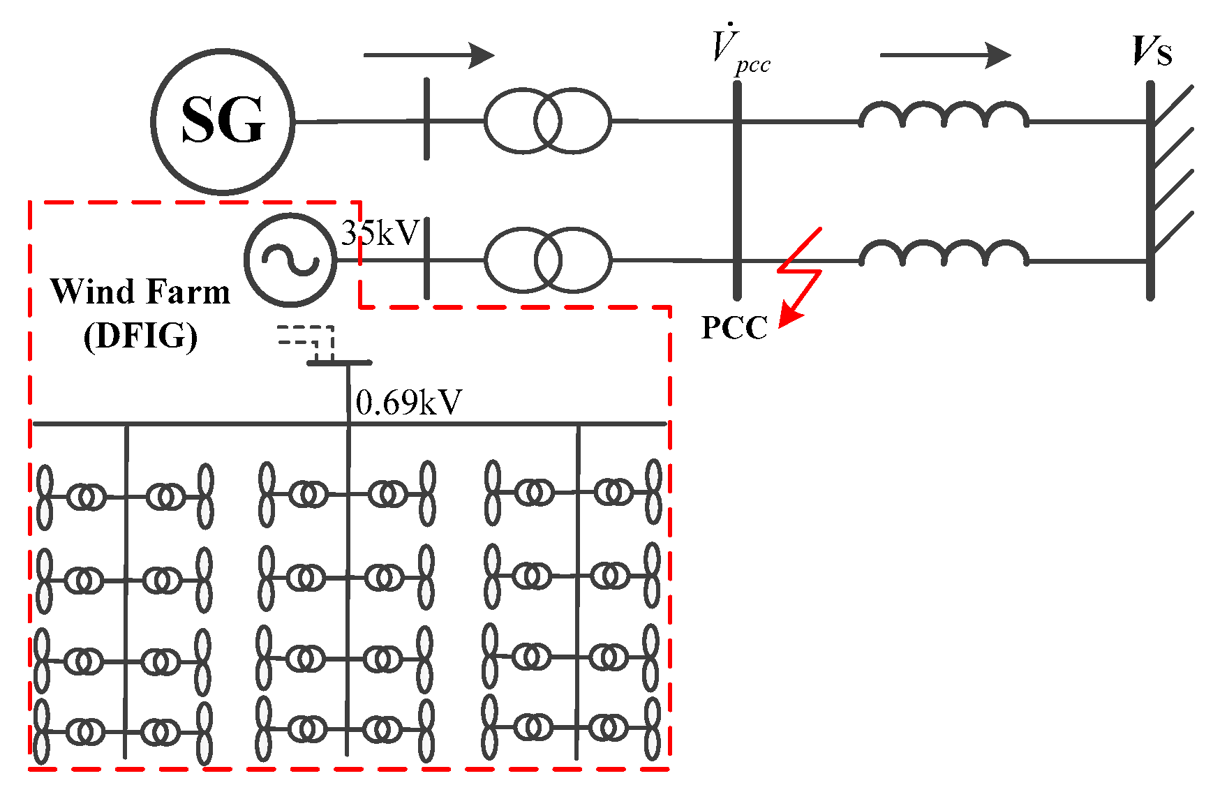
2.1. Power System Model

The paper considers a power network that includes both new energy power generation systems and traditional power generation systems. The PFC for this power system is consistent with the AC power flow of the traditional system. The nodal power deviation equation can be written as follows:
Δ P i = P i EG P i ED V i j i V j G i j cos θ i j + B i j sin θ i j
Δ Q i = Q i EG Q i ED V i j i V j G i j cos θ i j B i j sin θ i j
where P i and Q i are injected active power and reactive power, respectively. Moreover, θ i j indicates the corresponding voltage phase angle difference between i and j . P i EG and Q i EG represent the injection powers; P i ED and Q i ED are the energy consumed by the bus i electrical load. V i and V j denote the voltage of bus i and j. Finally, G i j and B i j are the conductance and admittance, respectively.
Voltage fluctuations occur due to system disturbances or when the voltage command is altered by dispatching at a higher level. In this case, power systems must adhere to the following voltage deviation limits from the grid point:
V pcc ref V pcc err V pcc V pcc ref + V pcc err
[ Q g i min , Q g i max ] = [ 0 , Q g i max ]   , V pcc ref > V pcc + V pcc band [ Q g i min , 0 ]   , V pcc ref < V pcc V pcc band
where V pcc is the current voltage, V pcc ref indicates the voltage control instruction, V pcc err represents the voltage error, and V pcc band represents the voltage control dead zone.
U i min U i U i max      i N S
Q sc i min Q sc i Q sc i max      i N Q
where V i max and V i min are the upper and lower limits of the voltage, respectively.

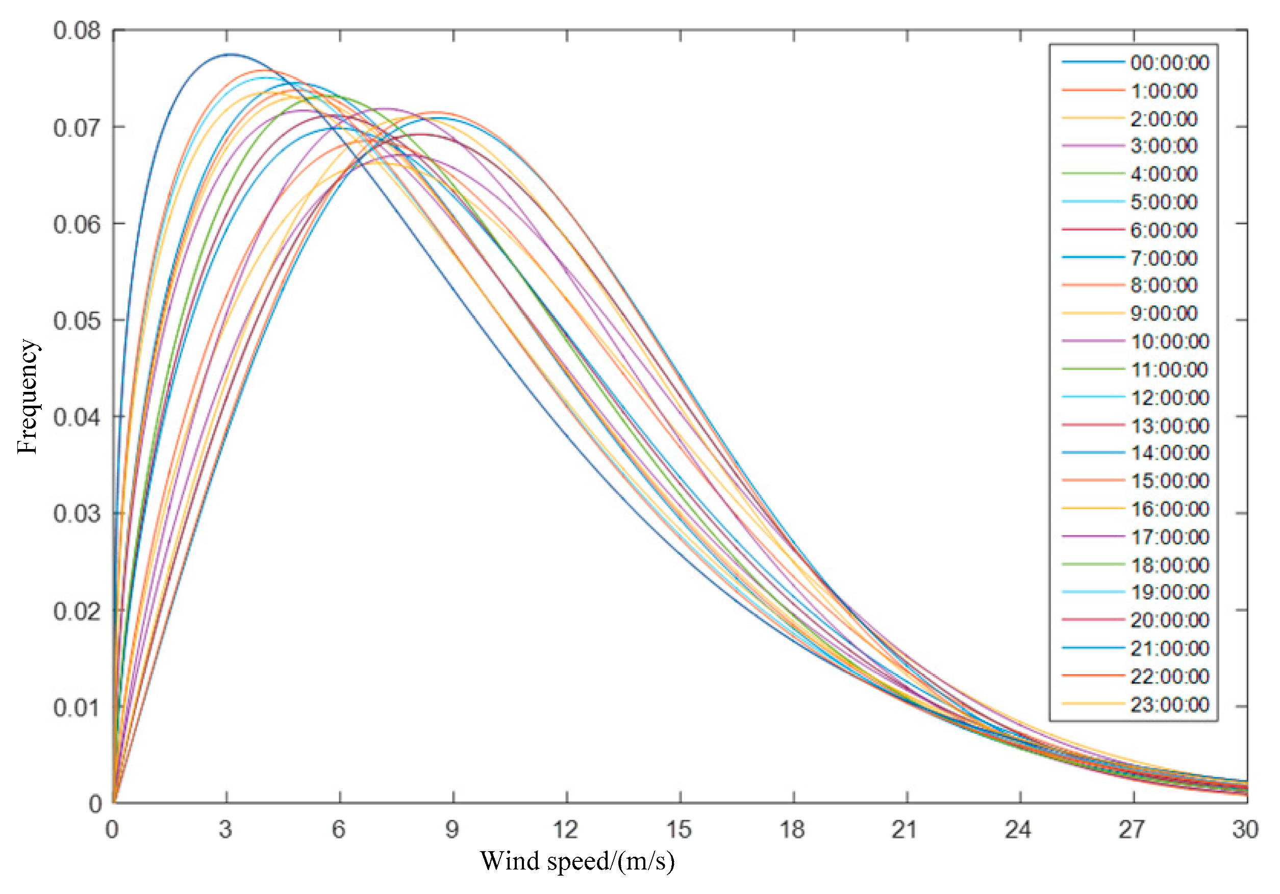
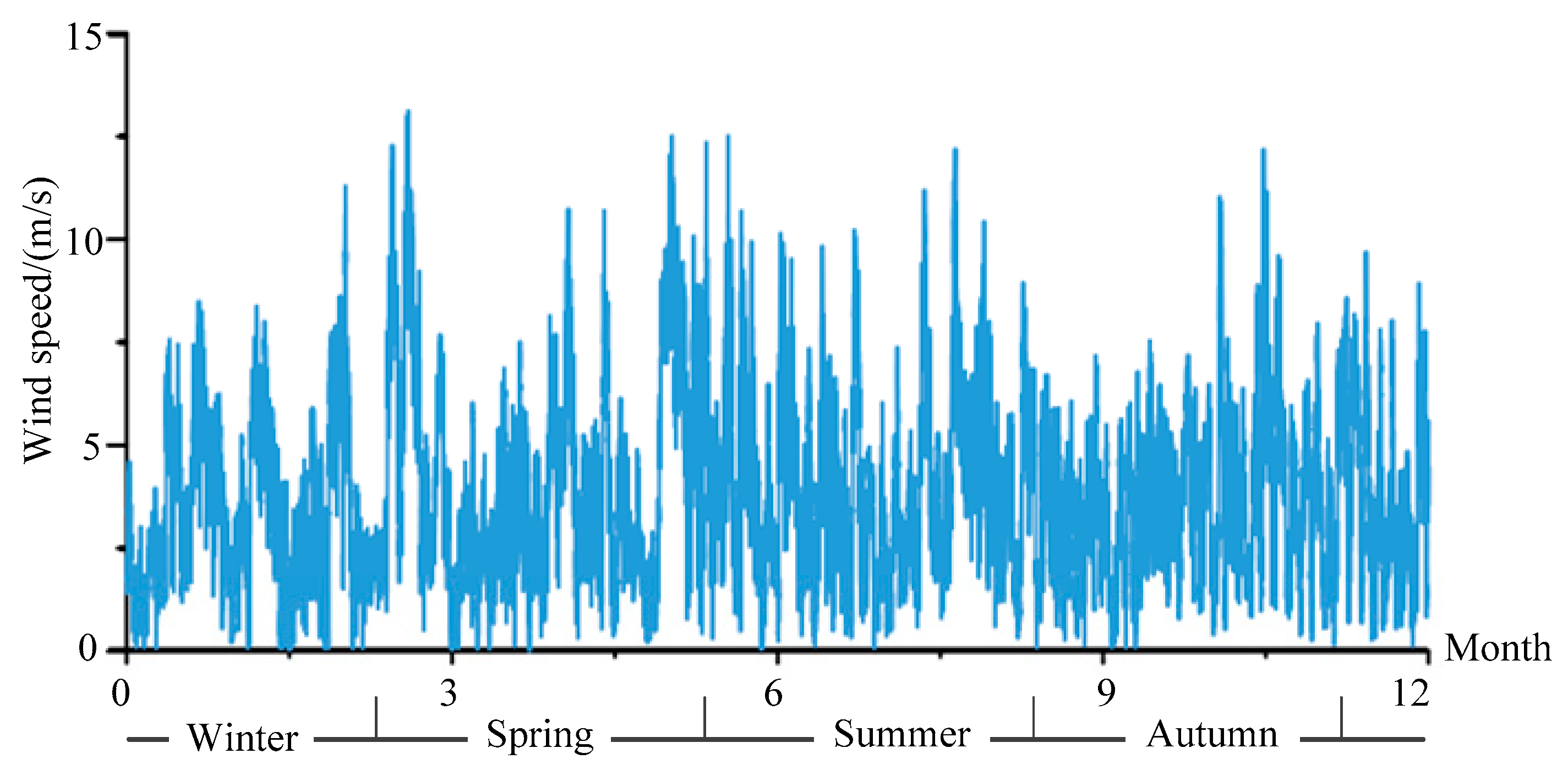
2.2. Uncertainty Model of Wind Power Output

The probability model of the wind turbine comprises two components: the wind speed model and the wind turbine model. Wind speed is affected by different factors, such as region, season, climate temperature, and geographical location, and has strong random volatility. When analyzing the PFC of the power system with new energy, the active output of the wind farm is calculated using the fan output characteristic curve. Wind speed is described by the high-precision fitting of the Weibull Distribution of wind speed change. Its PDF is shown in Figure 2.
During operation, an asynchronous generator is typically used with an inverter to generate an excitation magnetic field, which enables it to realize reactive power absorption and maintains the stable operation of the power grid. The probability model of wind turbine output power can be expressed as follows:
f P W , t ( P W , t ) = Pr ( P W t = 0 ) = 1 exp ( ( W S in c t ) k t ) + exp ( ( W S off c t ) k t ) Pr ( P W t = P WR = exp ( ( W S R c t ) k t ) exp ( ( W S off c t ) k t ) k t ( W S R W S in ) c t k t P WR W S in + P W t P WR ( W S R W S in ) k t 1 exp ( W S in + ( P W t / P WR ) ( W S R W S in ) c t ) k t 1 ,   else
( P W i , tur , t P W i , t ) = P W i , t P WR i ( P W t P W i , t ) f P W t ( P W t ) d ( P W t ) + Pr ( P W t = P WR ) ( P WR P W i , t ) ( P W i , t P W i , t ur , t ) = 0 P W i , t ( P W i , t P W t ) f P W t ( P W t ) d ( P W t ) + Pr ( P W t = 0 ) P W i , t
where W S in is the cut in wind speed, W S off symbolizes cut out wind speed, W S R denotes rated wind speed, and P WR represents rated output power. In addition, k t is the shape parameter at time t, and c t is the scale parameter reflecting the average wind speed of the wind field, m/s. PWi,t is the actual output of ith wind farm at t time.

3. Mathematical Model of DSSR

A power system’s DSSR is a node injection power space comprising the active and reactive power injected by all power system nodes. The boundary of a dynamic security and stability margin is uniquely determined by the network topology of the system, and remains constant regardless of the operating state, such as node injection. The DSSR boundary only needs to be calculated once for the given network topology and a predetermined contingency value. Then, its hyperplane coefficient is stored in the database for online use in the future, without increasing the computational burden of online use.

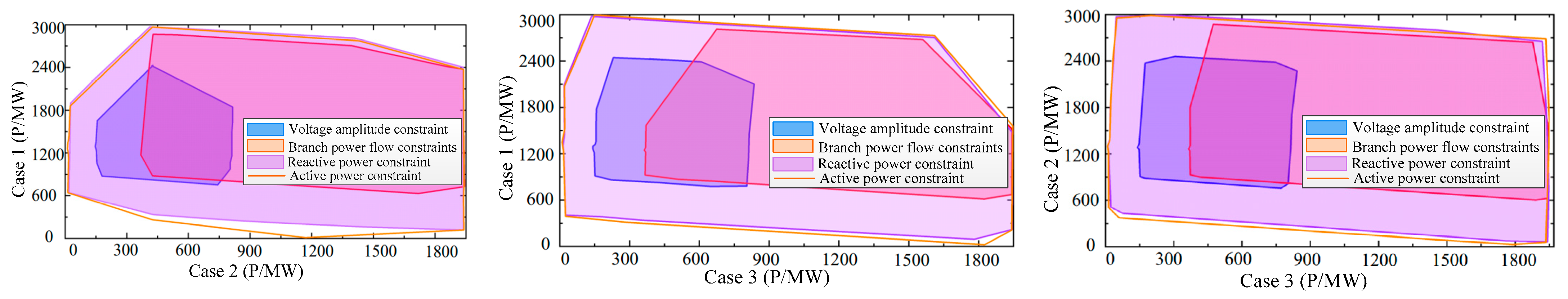
3.1. Security Constraints and SSR of the Grid

The grid nodes are divided into generator G and load L. The voltage limitation set is specified as follows:
M V r : = M V L r × M V G r
Among these,
M V L : = V L V L min V L V L max V L R n n 0
M V G : = V G V G min V G V G max V G R n 0
Letting Θ k M = α i α j be the voltage phase angle variation between nodes i and j at both ends of the branch, the power system’s line current limitation can be presented as follows:
M Θ r : = M Θ T B × M Θ L B
Among these,
M Θ T B : = Θ T B Θ T B M Θ T B Θ T B M
M θ L B : = Θ L B Θ L B M Θ L B Θ L B M
Θ T B R n , Θ L B R n b n
Suppose PiM and Pim represent the maximum and the minimum permissible limits of Pi. In this case, the constraint set satisfying (V, Θ) is as follows:
M P : = V , Θ P i m P i V , Θ P i M , i G
Among these,
V = V G V L ,   Θ = Θ T B Θ L B
The set M described by the coordinates (V, Θ) can be represented as follows:
M V L r : = Δ V L R n n 0 V L m V L 0 Δ V L V L M V L 0
M V G r : = Δ V G R n 0 V G m V G 0 Δ V G V G M V G 0

3.2. DSSR Boundary of Power System

There are two hypotheses regarding the SSR of the power grid [18], as follows:
Hypothesis 1. 
Only the DSSR of active power needs to be studied.
Hypothesis 2. 
In the injected power space, the DSSR must satisfy the following inequality because the active power injection of the generator  P u is always positive, and the active power injection of the load  P v is always negative:
P u 0 ,   P v 0
The structure of a power system with short-circuit fault can be divided into three stages:
Before, during, and after the accident.
d x d t = f a x ,   < t < 0 d x d t = f b x ,   0 < t < τ d x d t = f c x ,   τ < t < +
where a, b, and c represent the pre-fault, fault-time, and post-fault network topologies, respectively, and τ is the time constant for the short circuit fault.
After a specific type of short-circuit defect, the given power system’s architecture is transiently stable if the injected power vector y (including the active power injection Pi of three units) is stable. Dynamic security stability describes this condition, and the injected power y is safe. In the realm of injected power, the DSSR looks like this:
Ω d a , b , c : = y x d y A y Y l
where xd(y) is the fault-clearing state, A(y) indicates the SSR around the equilibrium point given by injection y in the state space after the fault, and Yl is the constraint set of the maximum and minimum limits of the injection power space of each node.

3.3. Hyperplane Equation Construction

The DSSR is composed of critical hyperplanes, and the hyperplane equation can be expressed as follows:
s = 1 n α s P s = 1
where Ps is the system’s sth active power injection, and αs indicates the hyperplane coefficient that corresponds to Ps.
According to hyperplane approximation, the DSSR can be expressed as follows:
Ω d : = P R n s = 1 n α s P s 1 P s m P s P s M s = 1 , 2 , , n
The following equation is the DSSR boundary fitting error:
E r r D S R = i = 1 n α i P i 1 i = 1 n α i 2 i = 1 n P i 2

4. Study of the AVURPSO-RLS Approach for Hyperplane Fitting

This paper combines the intercept and AVURPSO-RLS methods to calculate the hyperplane coefficient of the security domain and then obtain the DSSR of the new energy power system.

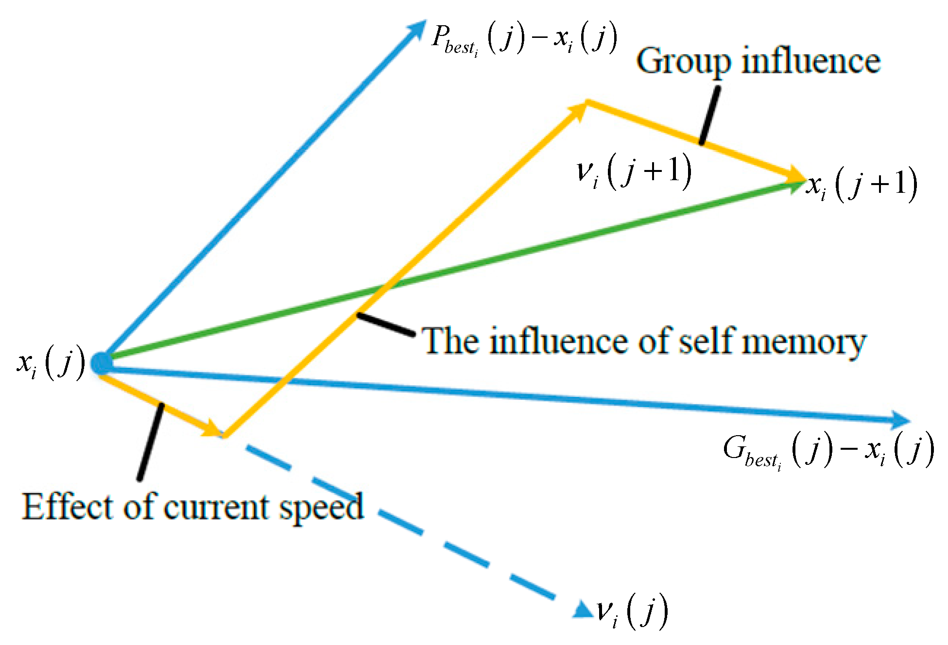
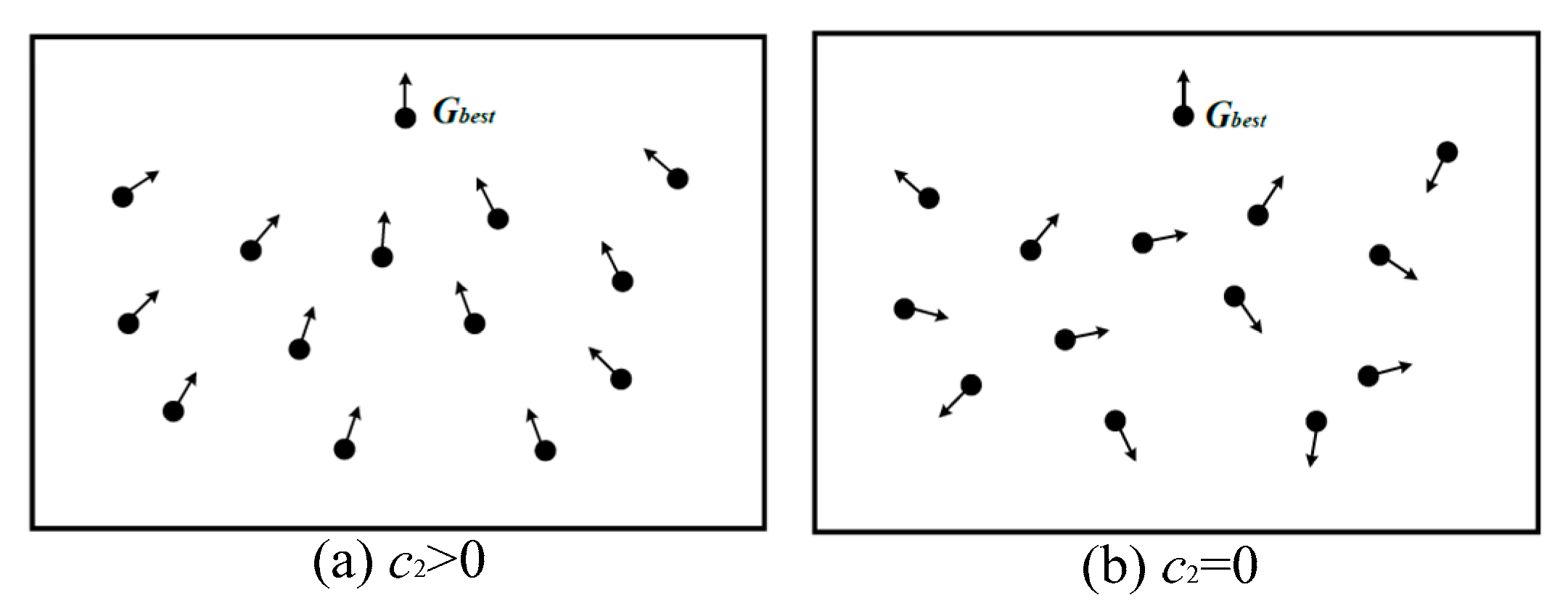
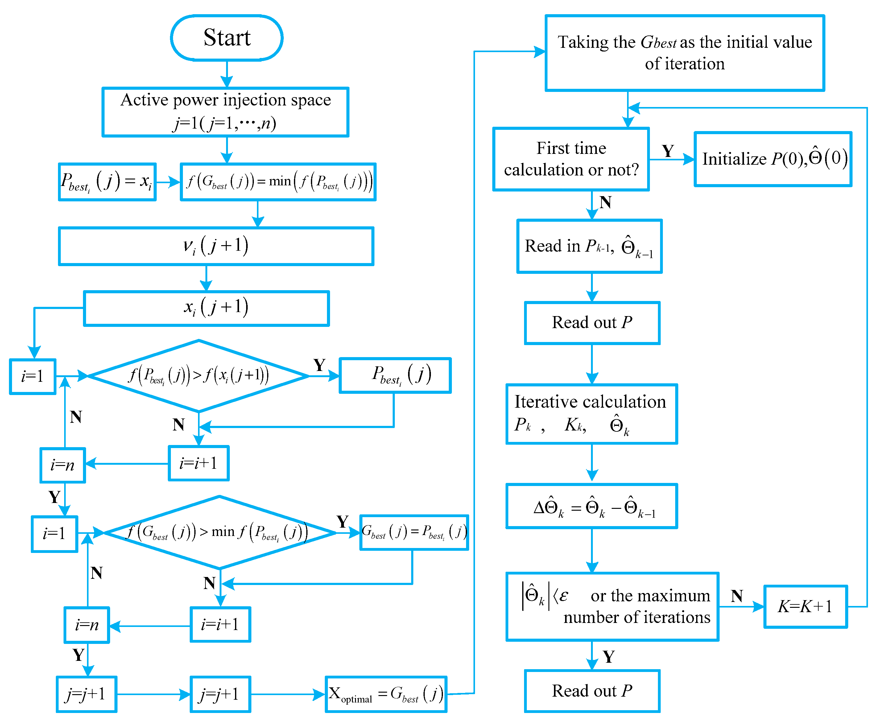
4.1. AVURPSO Algorithm

The novelty of the present study lies in finding the global optimum of the injection power value at the best level using an adaptive velocity update relaxation particle swarm optimization, namely, AVURPSO, with a higher convergence speed and more accurate response than the basic particle swarm optimization (PSO) algorithm seen in Figure 3. The individuals of the PSO algorithm are referred to as particles, and the positions of particles within the search space are changed based on each of the individuals’ social–psychological tendencies to delete others. Specifically, the velocity (v) and position (x) of each particle will be changed by the particle’s best value (Pbest) and the global best value (Gbest), as follows:
v i j + 1 = ω v i j + c 1 r 1 P b e s t j x j + c 2 r 2 G b e s t j x j
x i j + 1 = x i j + v i j + 1
ω = ω max ω max ω min i ter , max
where vi(j + 1) represents particle i’s velocities at iteration j, and xi(j + 1) indicates particle i’s locations at that iteration. Moreover, ω is the inertia weight used to regulate the effect of past velocity history. In this equation, t represents the number of iterations, c1 represents the learning factor for cognitive abilities, c2 is the learning factor for social abilities, and r1 and r2 are random values with uniform distribution across [0, 1]. Particles’ uncontrolled excursions beyond the search space may often be quelled by limiting the value of each component in v to fall inside the interval [vmin, vmax]. Typically, particles’ velocities in classic PSO are capped at a value between [vmin, vmax]. The default values for vmin and vmax are xmin and xmax, respectively. The particle locations are listed inside the interval [xmin, xmax].
In AVURPSO, the velocity of each particle remains unchanged if its fitness at the current iteration is superior to that at the preceding iteration. Otherwise, the particles’ velocities are updated as stated by [28], thereby improving computational efficiency. The new position of the particle is then calculated by [33]:
x i j + 1 = 1 m f x i j + m f v i j + 1
If c1 and c2 are kept modest, the particle may travel a greater distance before being dragged back. In contrast, using high values accelerates progress, but may compromise the ability to reach the designated areas. Therefore, c1 and c2 are presented as:
c 1 = i t e r max i t e r × c 1 b c 1 a i t e r max + c 1 a
c 2 = i t e r max i t e r × c 2 b c 2 a i t e r max + c 2 a
where c1b and c2b are the beginning and ending values of constants c1 and c2, and c1a and c2a are the constants’ intermediate values. In reality, the optimal solutions are usually identified throughout the search interval, including values for c1 from 2.5 to 0.5 and c2 from 0.5 to 2.5. When c1 is set to a high value and c2 is set to a small value, particles are free to roam the search space rather than converging on the (Pbest)i. Late in the optimization, when c1 is small and c2 is big, the particles converge to (Gbest)i. The convergence speeds of PSO and AVURPSO algorithms are shown in Figure 4.
The momentum factor, mf, has a value between 0 and 1. Take the following equation as an example of an adaptive modification made to the momentum factor:
m f = i t e r max i t e r × m f 2 m f 1 i t e r max + m f 1
where mf is decreased from the maximum value mf1 to the minimum value mf2.
As shown in Figure 5, the objective function for Gbest converges in the PSO, IPSO, VURPSO and AVURPSO algorithms. This figure shows that using the PSO as an objective function leads to convergence values of 0.00334, 0.00335, 0.00325, and 0.00323 for Gbest in the PSO, IPSO, VURPSO and AVURPSO algorithms, respectively. Therefore, AVURPSO is a superior algorithm to the other three. The following shows summaries of the case studies presented in this paper.

4.2. Recursive Least Square (RLS) Method

The least square (LS) method is the most basic and widely used method, and was first proposed by Gauss (k. f. Gauss) in his research on orbital motion orbit prediction. The RLS is a newly developed method based on the LS method [14]. The RLS can be obtained as follows:
To represent the L-group observations of an observable system, the symbol y i R , y i R n , i = 1 , 2 , , L is used to satisfy y i = x i θ as below:
y 1 y 2 y k = ϕ 1 T ϕ 2 T ϕ k T Θ
where k represents k groups of observed data; y i represents the output observation of the ith group of data. ϕ i T = x 1 i , x 2 i , , x n i R 1 × n ; Θ = θ 1 θ 2 θ n R n × 1 indicates the input observation value of the ith group of data.
where Φ k = ϕ 1 T ϕ 1 T ϕ 1 T R k × n , Y k = y 1 y 2 y n R k × 1
Φ is the data vector matrix and Y is the system output matrix.
From this, at time k, the least squares estimate can be obtained.
Θ ^ = Φ k T Φ k 1 Φ k T Y k
where
P k 1 = Φ k T Φ k
because
P k 1 = Φ k T Φ k = ϕ 1 , ϕ 2 , , ϕ k ϕ 1 T ϕ 2 T ϕ k T = i = 1 n ϕ i ϕ i T = i = 1 n 1 ϕ i ϕ i T + ϕ k ϕ k T = P k 1 1 + ϕ k ϕ k T
Therefore,
P k 1 = P k 1 1 + ϕ k ϕ k T
Φ k T y k = Φ k 1 T y k 1 + ϕ k y k
Θ ^ k = Φ k T Φ k 1 Φ k T y k = P k Φ k T y k = P k Φ k 1 T y k 1 + ϕ k y k
because
Θ ^ k 1 = P k 1 Φ k 1 T y k 1
Therefore,
P k 1 Θ ^ k = ϕ k ϕ k T
At time k, this can be expressed as
Θ ^ k = P k Φ k 1 T y k 1 + ϕ k y k = P k P k 1 Θ ^ k 1 + ϕ k y k = P k P k 1 Θ ^ k 1 ϕ k ϕ k T Θ ^ k 1 + ϕ k y k = Θ ^ k 1 + P k ϕ k y k ϕ k T Θ ^ k 1 = Θ ^ k 1 + K k ε
Then the LS estimate can be given as
ε k = y k ϕ k T Θ ^ k 1 Θ ^ k = Θ ^ k 1 + K k ε K k = P k ϕ k P k = P k 1 1 + ϕ k ϕ k T 1
where
P k = P k 1 1 + ϕ k ϕ k T 1 = P k 1 P k 1 ϕ k 1 + ϕ k T P k 1 ϕ k 1 ϕ k T P k 1 = P k 1 P k 1 ϕ k ϕ k T P k 1 1 + ϕ k T P k 1 ϕ k
The iterative formula for the RLSM is given as follows:
ε k = y k ϕ k T Θ ^ k 1 Θ ^ k = Θ ^ k 1 + K k ε K k = P k ϕ k P k = P k 1 P k 1 ϕ k ϕ k T P k 1 1 + ϕ k T P k 1 ϕ k

4.3. The AVURPSO-RLS Parameter Identification

Although achieving accurate ranging in the AVURPSO algorithm is challenging, its global optimization capacity helps to narrow the solution range and approximate the optimal solution. The main drawback of the RLS is its sensitivity to the initial iteration value. However, when the initial value of the iteration is closer to the real solution, the RLS exhibits higher convergence speed and accuracy. Therefore, combining the global optimization ability of AVURPSO with the fast convergence ability of the RLS in the neighborhood of the global optimal solution can help us achieve the desired results. The flowchart for finding the global optimal DSSR process based on the proposed AVURPSO-RLS algorithm is depicted in Figure 6.

5. Case Study

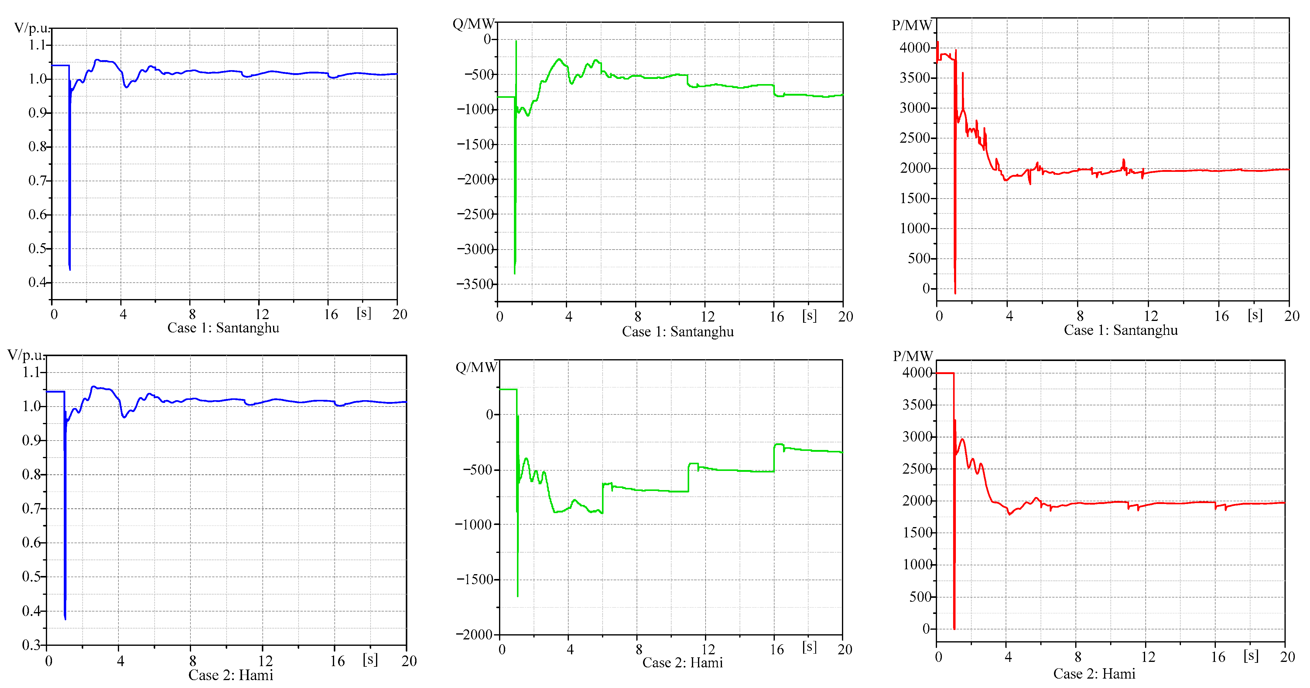
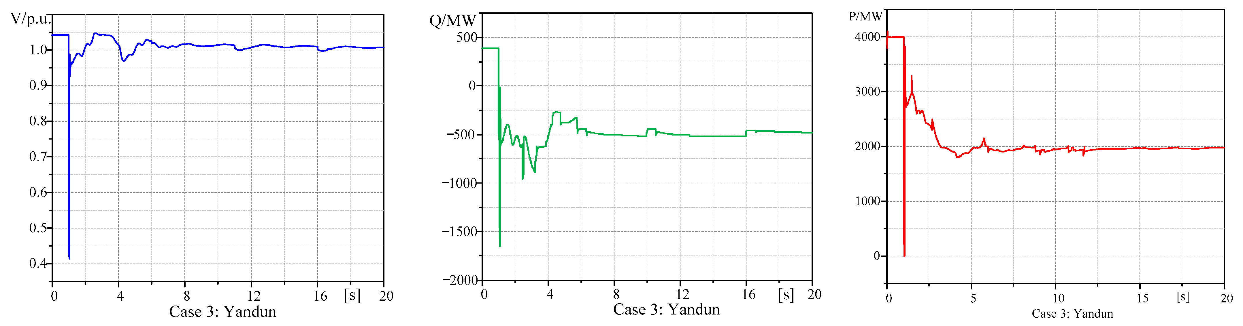
5.1. Time Domain Simulation of DSSR

In this section, the suggested approach of AVURPSO-RLS is tested on an actual power grid in Hami City, China—a city with abundant new energy and coal energy resources on the Chinese mainland. Despite the abundance of new energy resources in this region, their shortcomings, such as their stochastic nature, volatility, and load distribution, present challenges for large-scale utilization. Generally, the wind speed here is greater than 4.38 m/s, and the effective wind speed is more than 2000 h. The typical output curve of wind energy in western China is shown in Figure 7.
In addition, Hami is one of the major coal bases in China. It was the first UHVDC transmission channel in China to combine new energy with thermal electricity. The DIgSILENT/Power Factory software was used to develop and test the Hami power grid.
As can be seen in Figure 8, the three wind farm stations in this grid are Santanghu, Hami, and Yandun. This article analyzes three versions of the Hami Power Grid based on the geographic locations of wind farms.
(1)
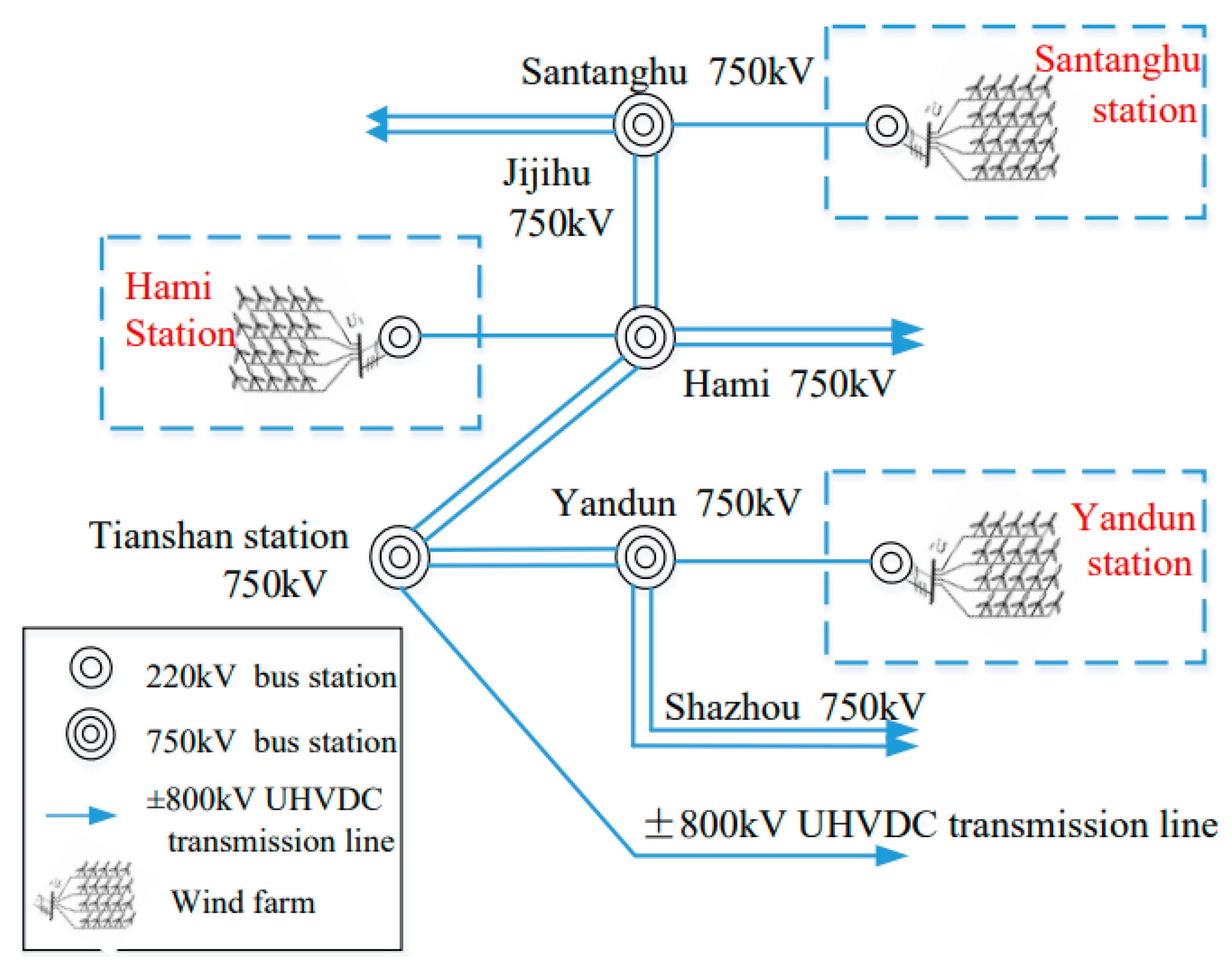
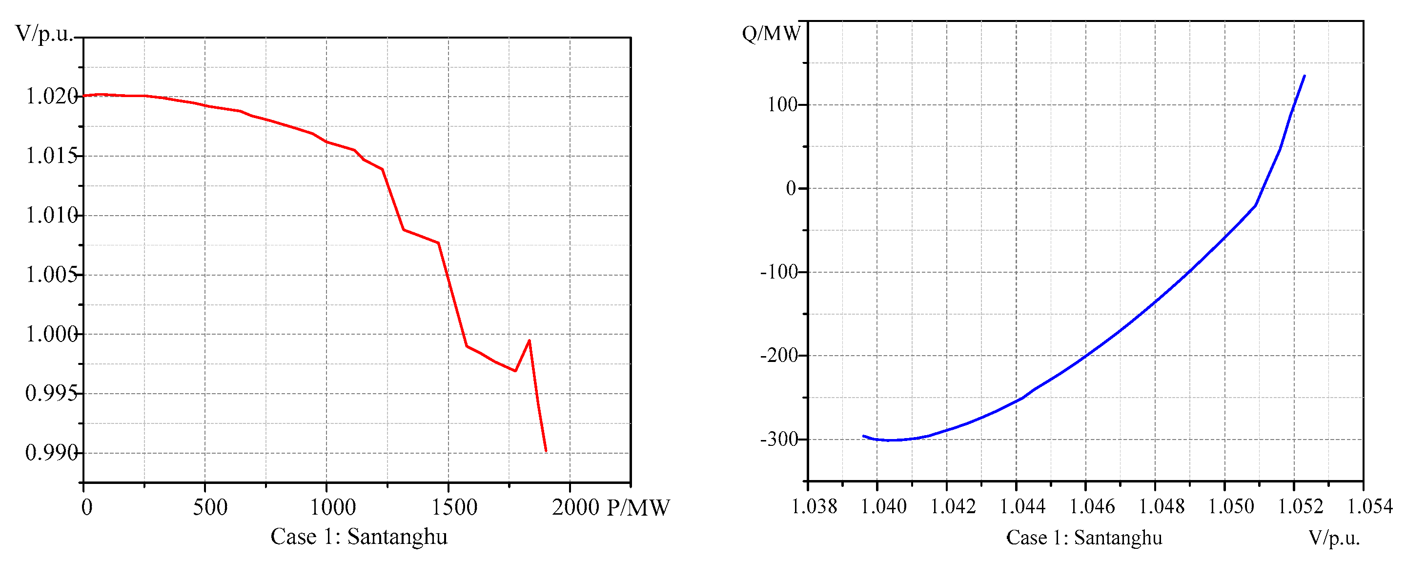
Case 1: Santanghu station encompasses six wind farms and uses 220 kV wires to link the wind farms to its 750 kV station.
(2)
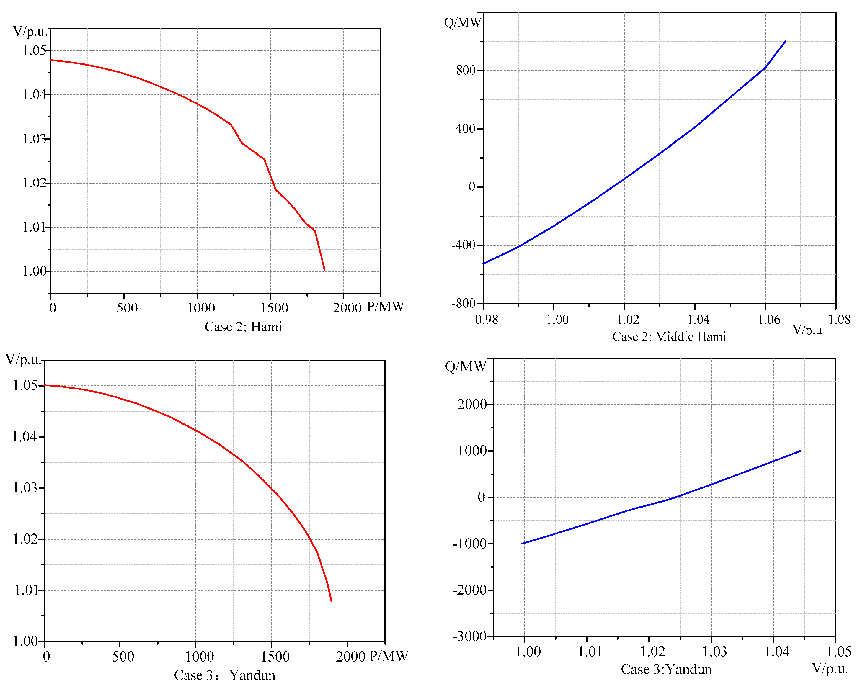
Case 2: Three major wind farms (220 kV) are linked to the 750 kV central Hami station through three (220 kV) main wind farms.
(3)
Case 3: Five (220 kV) primary wind farms are linked to the 750 kV Yandun station. Consequently, this paper discusses the three wind farms affiliated with the Hami Power Grid.
Figure 9 depicts the normal operating state curves (PV and QV curves) of the three wind farms. The figure displays the PV and QV curves at a certain time in the three cases of Hami power grid operation under normal conditions. As can be seen, the outputs of P and Q are within the stable voltage range [0.95~1.05].
The bus B2 of the Hami power grid is intentionally subjected to a three-phase short-circuit fault. The fault is initiated at 1 s and cleared at 1.1 s. Figure 10 illustrates the equivalent dynamic response of the system. A three-phase short circuit fault occurs one minute after the system starts to operate. After the fault is removed, the system transitions to a new stable operating state through adjustment.
After the failure, the P, Q, and V all drop significantly at the same time. As the P stabilizes, the V rises, and the Q increases after the fault has been cleared.
Based on Figure 9 and Figure 10, a two-dimensional security domain for three cases is obtained through the AVURPSO-RLS algorithm.
Boundary data can be obtained from the two-dimensional security and stability regions of the three cases shown in Figure 11, and the dynamic security and stability region of the system can be obtained via HP fitting.
The HP approach can be used to match the DSSR boundary via extensive simulation computations, and the HP coefficients can be discovered using AVURPSO-RLS. Then, DIgSILENT/Power Factory simulation is utilized to derive the various p values of the three situations. Three of these examples’ DSSRs are shown in Figure 12.
The P of the three regions is used as the research object to obtain the DSSR surface, as shown in Figure 12. For this study, in the DSSR plane, the yellow area shows where the system can operate safely and stably. The area extending from yellow to red and yellow to blue ensures the system’s safe and stable operation. The dark red and dark blue areas allow the system to operate safely and stably under normal conditions, but their safety and stability may be reduced in cases of system failure. According to the above simulation, the active output limit in the Santanghu area is 1833.6 MW, that in Hami is 4742.22 MW, and that in Yandun is 5888.3 MW. Combined with the power flow calculation data, the active power margin Kp of each region is 5.7%, 65.4%, and 15.8%, respectively. The reactive power output limit in the Santanghu area is 2641.2 MW, while it is 1656.7 MW in the Hami area, and 827.0 MW the Yandun area. Combined with the tidal current calculation results, the reactive power margin KQ values of each wind zone are 25.6%, 40.7%, and 37.1%, respectively. The voltage fluctuation amplitude in the Santanghu area is [0.44, 1.055], while it is [0.37, 1.06] in Hami and [0.42, 1.045] in Yandun. As the P of each region gradually increases beyond the limit, the operating point will also move to the upper part of the DSSR surface, and the wind farm may collapse, leading to insecurity in the entire Hami power grid. When the system’s operating point is above the DSSR surface, excessive reactive power output in each region can easily cause an imbalance in the system’s power.
The different proportions of the calculation error of the HP coefficient in the injection power space for the three cases are shown in Figure 13. When the injection power is 70%, the error of the HP coefficient is the smallest, and the fitting plane has high precision and reliability. The maximum fitting error of the boundary of the DSSR obtained by fitting is 4.56% (here, the error is defined as the maximum ratio of the coordinate component of the distance from the critical point to the fitting hyperplane to the coordinate component of the corresponding point on the hyperplane; that is, the percentage). All results meet the requirements of engineering precision.
To improve the efficiency when creating a DSSR boundary with a hyperplane expression, the AVURPSO-RLS technique is suggested as a viable alternative. The first step involves looking for critical points in an equivalent effective search space built from the key generators identified by the AVURPSO algorithm and the orthogonal point selection method. The second step involves using the RLS method to fit the hyper-plane coefficients of the DSSR boundary. Extensive simulation results regarding the Hami power grid demonstrate that the proposed technique is much more computationally efficient than the existing fitting method, without sacrificing accuracy.

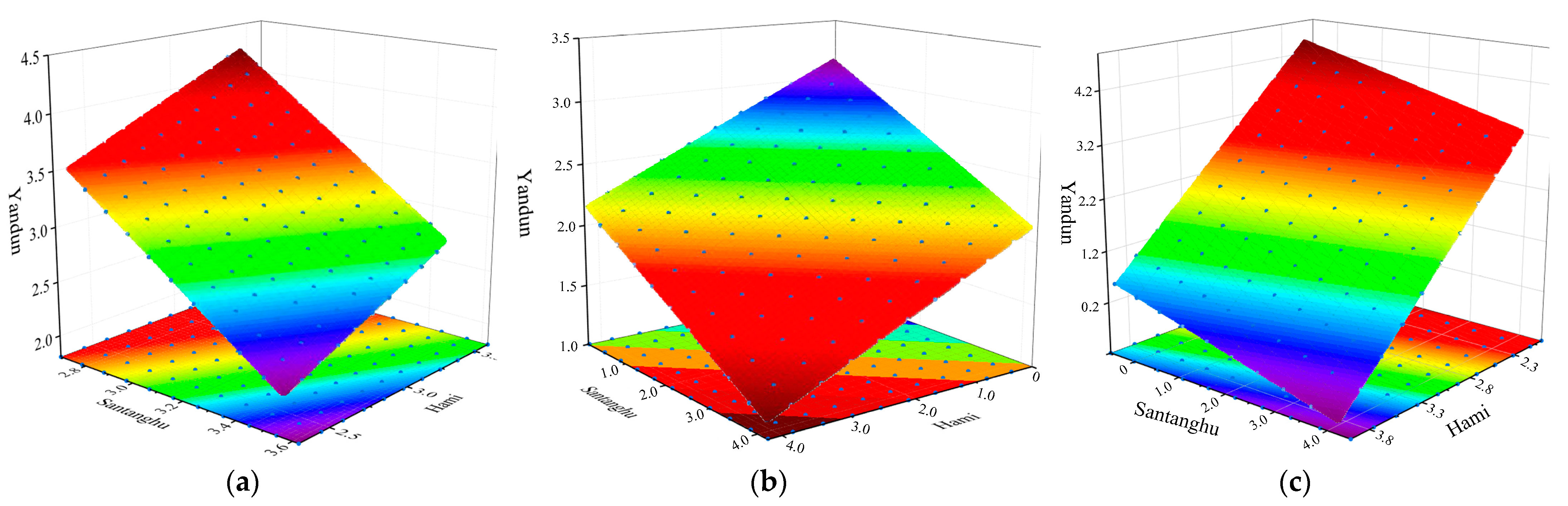
5.2. Sensitivity Analysis of DSSR

Sensitivity analysis is used to verify whether the IPSO-RLS hybrid algorithm is applicable and whether the static security domain is stable, that is, whether previous analysis results will change when the research object undergoes minor changes. In actual analysis work, partial adjustments can be made to the analysis results based on changes in the analysis parameters, and new analysis results can be obtained without recalculation. In this paper, several representative critical points are selected to perform sensitivity analyses of ±10%, ± 20%, and ± 30% on the critical surfaces of the DSSR, respectively, in order to simulate fluctuations in wind speed. The results are shown in Figure 14.
When the operating points of the system under different outputs are within the DSSR and below the DSSR surface, the system is safe. Otherwise, the system is not secure. The sensitivity analysis results in Figure 14 indicate that the operating points corresponding to different sensitivity changes are within the limits of the output range of each wind farm group, and the entire system is still safe; that is, the DSSR surface is not sensitive to sensitivity changes. Therefore, the IPSO-RLS hybrid algorithm is reasonable and applicable for use in DSSR analysis.

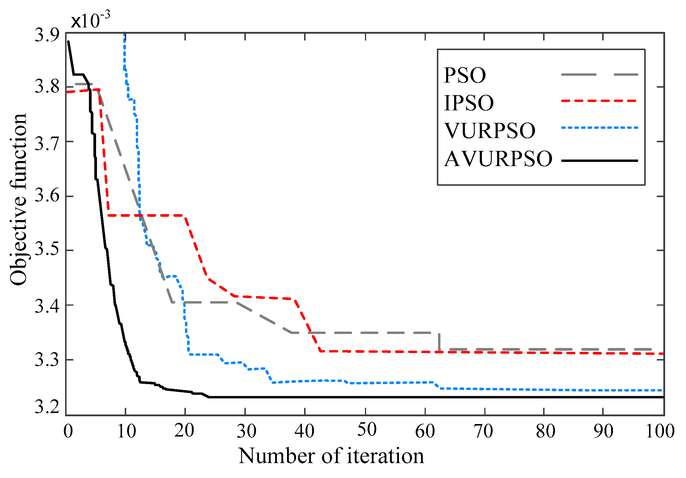
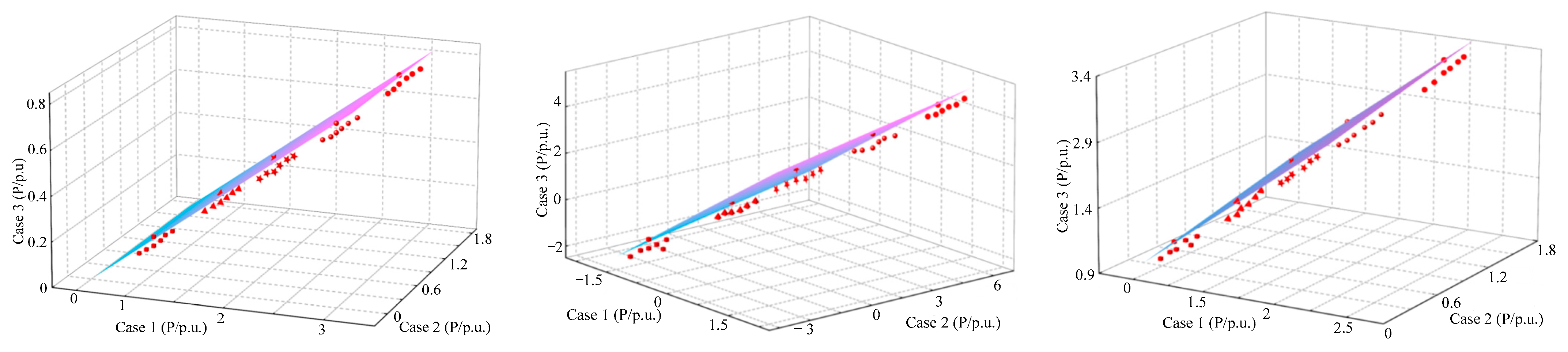
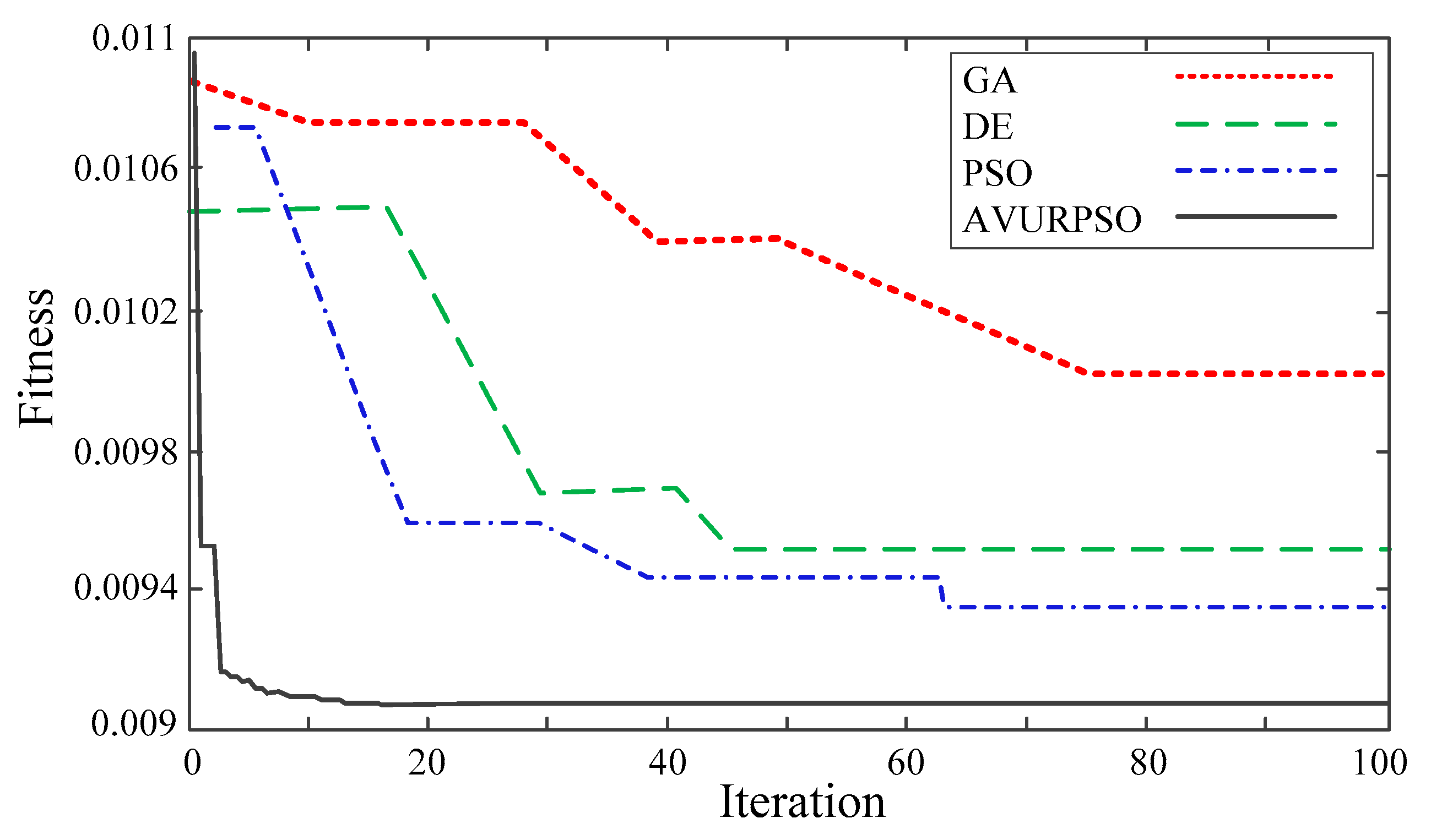
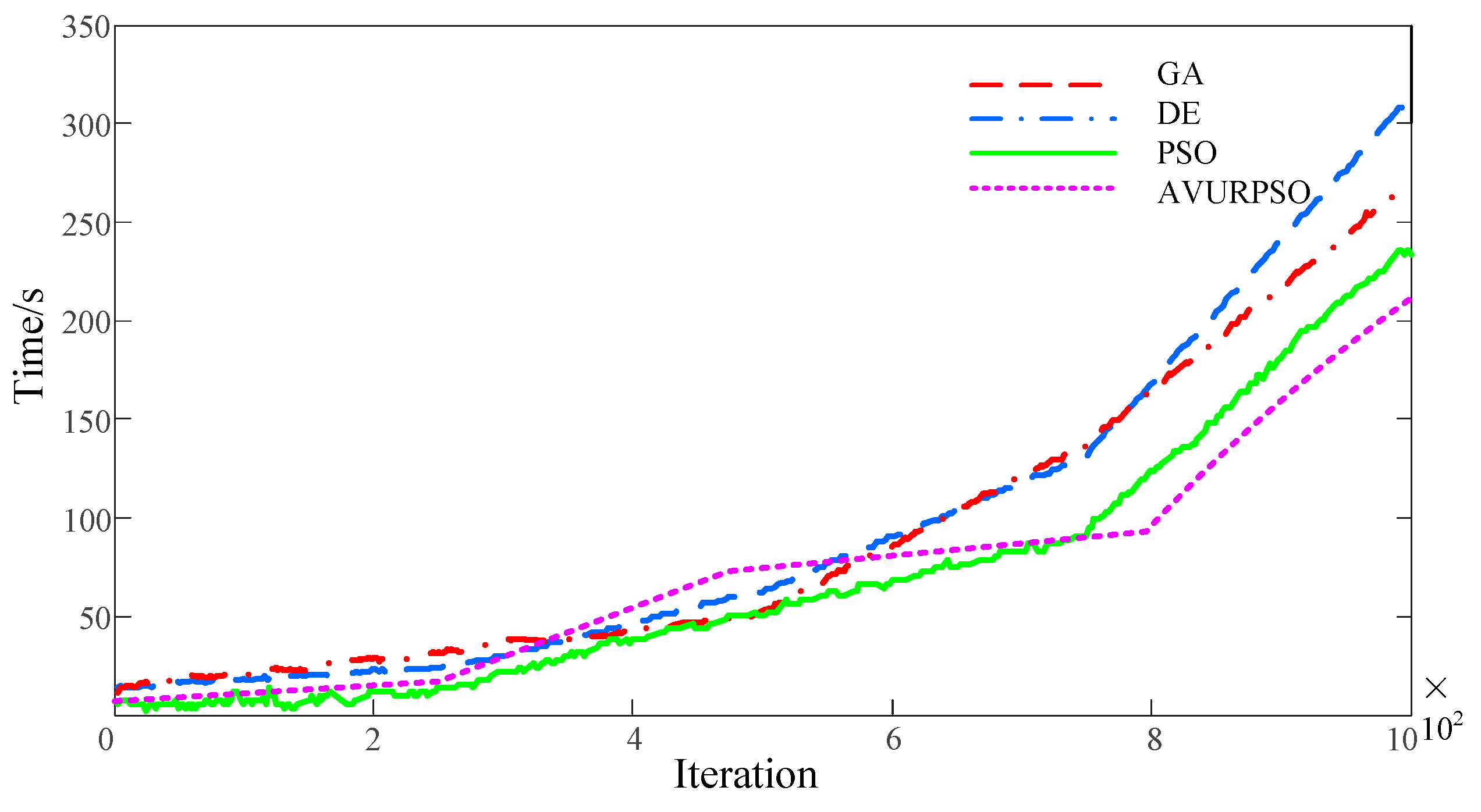
5.3. Comparative Analysis of Algorithms

To verify the effectiveness and accuracy of the proposed AVURPSO algorithm, the error and convergence accuracy are compared with the genetic algorithm (GA), the different evolutional algorithm (DE), and the PSO algorithm. During the experimental verification, the control parameters of all algorithms are set according to Table 1.
Figure 15 compares the convergence accuracies of the GA, PSO, DE, and AVURPSO algorithms when used in optimization. The error comparison results of the GA, PSO, DE, and AVURPSO algorithms are listed in Table 2.
The “best value”, “worst value”, “average value”, and “standard deviation” in Table 2 represent the errors in the best value, the worst value, the average value, and the standard deviation value of the P obtained in the search space. The GA and DE algorithms cannot find the optimal error solution under the different conditions of new energy permeability. Although the results obtained by PSO are better than those obtained by the first two algorithms, the AVURPSO algorithm achieves higher accuracy with a smaller error. Therefore, it can be proven that the AVURPSO algorithm achieves the best performance in searching for the optimal solution.
The results show that the AVURPSO algorithm outperforms other algorithms in terms of accuracy, with its optimal solution (Best) being more accurate than those obtained by other algorithms. Additionally, AVURPSO exhibits a superior global or near-global optimal solution-searching ability. Moreover, the low standard deviation of the AVURPSO algorithm proves its stable consistency and higher convergence accuracy. The average global or near-global optimal solution yields a stable average P, further validating the AVURPSO algorithm’s reliability in producing high-quality solutions.
Figure 15 demonstrates that the AVURPSO algorithm has better convergence accuracy than the GA, DE, and PSO algorithms. The training results of the AVURPSO algorithm converge rapidly after 400 iterations, whereas the results of the PSO algorithm converge after 800 iterations. The GA algorithm seems to be the slowest, with an unstable and fluctuating iterative process, taking more time to converge successfully. Consequently, the AVURPSO algorithm is more efficient, and its strong exploration ability effectively overcomes its premature convergence and maintains its convergence speed.
The results in Figure 16 show that the AVURPSO algorithm takes less time to iterate, and is faster than the DE, GA, and PSO algorithms. The AVURPSO algorithm is more precise and faster in terms of convergence. In addition, the AVURPSO algorithm also shows improved precision in SSR compared with PSO.

6. Conclusions

This paper proposes the concepts and a model of the new energy power system DSSR. Since the operating parameters can be maintained within the constraints of the new energy DSSR, areas where operating parameter verifications can be simplified were further established, and this could improve the calculation speed. Then, a security and stability analysis framework for a new regional energy power system based on the DSSR was given. Based on the DSSR, a model for optimizing control was presented to adjust the system’s security status. The case study has verified the effectiveness of the security region and realized its visualization in a three-dimensional space. Furthermore, the secure operating point could be optimized to enhance the security and efficiency status under optimizing control. The proposed method pushes forward the process of the practical application of DSSR to enhance situational awareness, considering the uncertainty of new energy. In the future, the impact of the load can be further considered, and advanced data-driven methods can be further explored to improve the efficiency.
Based on the facts that HPs can approximate the boundaries of the practical SR in the power injection space, and that the SR is irrelevant to the operation state, the great advantages of the SR method when used in security monitoring, probabilistic security (risk) assessment, and the optimization of power systems have been discovered. Compared to the fitting method, the SR method significantly improves the computational speed. In addition, it achieves the accuracy required of practical engineering applications that require many simulations to search for their many critical points. In the future, the SR methodology will continue to be a powerful tool used in the security analysis of smart grids with massive and uncertain distributed generation capacities. Moreover, the SR methodology is a powerful tool for improving situation awareness, since it can make visualizations easier to construct, and enables the rapid determination of the security margin.

Author Contributions

Conceptualization, S.M.; methodology, S.M.; software, Q.Z.; validation, S.M., J.W. and Q.Z.; formal analysis, S.M.; resources, J.W.; data curation, S.M.; writing—original draft preparation, S.M.; writing—review and editing, S.M. and M.M.; supervision, W.W. and H.W.; funding acquisition, W.W. and H.W. All authors have read and agreed to the published version of the manuscript.

Funding

This work was supported in part by the National key research and development project sub project (2020YFC0827000), in part by the National Natural Science Foundation project (52067020), in part by the National Natural Science Foundation project (52267005), the Project supported by the Autonomous Region Natural Science Foundation (2020D01C068) and the National Natural Science Foundation of China (52167016).

Institutional Review Board Statement

Not applicable.

Informed Consent Statement

Not applicable.

Data Availability Statement

All data generated or analyzed during this study are included in the published article.

Acknowledgments

The authors would like to express their sincere gratitude to the experts for their unlimited support in the validation of the framework and for their suggestions, as well as for providing some data. The authors want to thank the editor and anonymous reviewers for their valuable comments and suggestions that have helped us to improve this article.

Conflicts of Interest

The authors declare that they have no known competing financial interests or personal relationships that could have appeared to influence the work reported in this paper.

References

  1. Zhu, H.; Goh, H.H.; Zhang, D.; Ahmad, T.; Liu, H.; Wang, S.; Li, S.; Liu, T.; Dai, H.; Wu, T. Key technologies for smart energy systems: Recent developments, challenges, and research opportunities in the context of carbon neutrality. J. Clean. Prod. 2022, 331, 129809. [Google Scholar] [CrossRef]
  2. You, Y.; Yi, L. Energy industry Carbon neutrality transition path: Corpus-based AHP-DEMATEL system modelling. Energy Rep. 2022, 8, 25–39. [Google Scholar] [CrossRef]
  3. Shabani, H.R.; Kalantar, M. Real-time transient stability detection in the power system with high penetration of DFIG-based wind farms using transient energy function. Int. J. Elect. Power Energy Syst. 2021, 133, 107319. [Google Scholar] [CrossRef]
  4. Boričić, A.; Torres, J.L.R.; Popov, M. Fundamental study on the influence of dynamic load and distributed energy resources on power system short-term voltage stability. Int. J. Elect. Power Energy Syst. 2021, 131, 107141. [Google Scholar] [CrossRef]
  5. Adetokun, B.B.; Muriithi, C.M.; Ojo, J.O. Voltage stability assessment and enhancement of power grid with increasing wind energy penetration. Int. J. Elect. Power Energy Syst. 2020, 120, 105988. [Google Scholar] [CrossRef]
  6. Wang, J.; Xu, J.; Liao, S.; Sima, L. Coordinated Optimization of Integrated Electricity-Gas Energy System Considering Uncertainty of Renewable Energy Output. Auto. Elect. Power Syst. 2019, 43, 2–9. [Google Scholar]
  7. Dong, X.; Tang, Y.; Bu, G.; Shen, C.; Song, G.; Wang, Z.; Zhao, B. Confronting problem and challenge of large-scale AC-DC hybrid power grid operation. Proc. Chin. Soc. Electr. Eng. 2019, 39, 3107–3119. [Google Scholar]
  8. Li, B.; Chao, P.; Li, W.; Xu, S.; Liu, X.; Li, Z. Transient overvoltage calculation method of wind power transmission system via UHVDC. Electr. Mach. Control. 2021, 25, 11–18. [Google Scholar]
  9. Tu, J.; Zhang, J.; Liu, M.; Yi, J.; He, Q. Study on Wind Turbine Generators Tripping Caused by HVDC Contingencies of Wind-Thermal-Bundled HVDC Transmission Systems. Power Syst. Technol. 2015, 39, 3333–3338. [Google Scholar]
  10. Wu, Y.; Hu, M.; Liao, M.; Liu, F.; Xu, C. Risk assessment of renewable energy-based island microgrid using the HFLTS-cloud model method. J. Clean. Prod. 2021, 284, 125362. [Google Scholar] [CrossRef]
  11. Hnyilicza, E.; Lee, S.; Schweppe, F.C. Steady-state security regions: Set-theoretic approach. IEEE Trans. Circuits Syst. 1982, 29, 703–711. [Google Scholar]
  12. Jarjis, J.; Galiana, F.D. Quantitative analysis of steady state stability in power networks. IEEE Trans. Power Appar. Syst. 1981, 1, 318–326. [Google Scholar] [CrossRef]
  13. Phillipe, V.G.; Saraiva, J.T. State-of-the-art of transmission expansion planning: A survey from restructuring to renewable and distributed electricity markets. Int. J. Elect. Power Energy Syst. 2019, 111, 411–424. [Google Scholar]
  14. Maihemuti, S.; Wang, W.; Wang, H.; Wu, J. Voltage Security Operation Region Calculation Based on Improved Particle Swarm Optimization and Recursive Least Square Hybrid Algorithm. J. Mod. Power Syst. Clean Energy 2021, 9, 138–147. [Google Scholar] [CrossRef]
  15. Lin, W.; Jiang, H.; Yang, Z. Time-line security regions in high dimension for renewable accommodations. arXiv 2022, arXiv:2201.01019. [Google Scholar]
  16. Zeng, Y.; Yu, Y. A practical direct method for determining dynamic security regions of electrical power systems. Proc. Int. Conf. Power Syst. Tech. 2002, 2, 1270–1274. [Google Scholar]
  17. Xue, A.; Wu, F.F.; Lu, Q.; Mei, S. Power System Dynamic Security Region and Its Approximations. IEEE Trans. Circ. Syst. 2006, 53, 2849–2859. [Google Scholar] [CrossRef]
  18. Yu, Y.; Liu, Y.; Qin, C.; Yang, T. Theory and Method of Power System Integrated Security Region Irrelevant to Operation States: An Introduction. Engineering 2020, 6, 754–777. [Google Scholar] [CrossRef]
  19. Zhang, Q.; Zheng, H.; Wang, J.; Liu, X.; Qu, Y.; Bie, Z. A method for calculating static voltage stability margin of power system based on aq bus. Power Syst. Technol. 2019, 43, 714–721. [Google Scholar]
  20. Xia, S.; Bai, X.; Chen, S.; Guo, Z.; Xu, Y. Solving for dynamic security region based on Taylor series trajectory sensitivity. Electr. Power Autom. Equip. 2018, 38, 157–164. [Google Scholar]
  21. Pourbehzadi, M.; Niknam, T.; Aghaei, J.; Mokryani, G.; Shafie-Khah, M.; Catalão, J.P.S. Optimal operation of hybrid AC/DC microgrids under uncertainty of renewable energy resources: A comprehensive review. Int. J. Elect. Power Energy Syst. 2019, 109, 139–159. [Google Scholar] [CrossRef]
  22. Javadian, S.; Haghifam, M.-R.; Firoozabad, M.F.; Bathaee, S. Analysis of protection system’s risk in distribution networks with DG. Int. J. Electr. Power Energy Syst. 2013, 44, 688–695. [Google Scholar] [CrossRef]
  23. Yu, Y.; Luan, W. Practical dynamic security region of power system. Proc. CSEE 1990, 13, 14–22. [Google Scholar]
  24. Yu, Y.; Lin, J. Practical analytic expression of power system dynamic security region’s boundary. J. Tianjin Univ. 1997, 30, 1–8. [Google Scholar]
  25. Zeng, Y.; Fan, J.C.; Yu, Y.X. Practical dynamic security regions of bulk power system. Auto. Elec. Power Syst. 2001, 25, 6–10. [Google Scholar]
  26. Min, L.; Yu, Y.X.; Lee, S.; Pei, T. Identification method of Instability modes and its application in dynamic security region. Auto. Electr. Power Syst. 2004, 28, 28–32. [Google Scholar]
  27. Feng, Z.; Yu, Y.; Zeng, Y. An Intercept method for determining practical dynamic security regions of power systems. Auto. Electr. Power Syst. 2006, 30, 18–22. [Google Scholar]
  28. Zeng, Y.; Yu, Y.X.; Jia, H.J. Computing practical dynamic security region by technology of power sensitivity analysis. J. Tianjin Univ. 2006, 39, 76–82. [Google Scholar]
  29. Qin, C.; Liu, Y.L.; Yu, Y.X. Dynamic security region of power systems with double fed induction generator. Trans. China Electro. Tech. Soc. 2015, 30, 157–163. [Google Scholar]
  30. Hou, K.F.; Yu, Y.X.; Lee, S.T.; Pei, Z. Reduction and reconstruction of power system practical dynamic security region. Auto. Electr. Power Syst. 2004, 28, 16–21. [Google Scholar]
  31. Russell, S.J.; Norvig, P. Artificial Intelligence: A Modern Approach; Pearson Education Limited: London, UK, 2016. [Google Scholar]
  32. Movahedi, A.; Niasar, A.H.; Gharehpetian, G.B. Optimal real-time operation strategy for microgrid: An ADP-based stochastic nonlinear optimization approach. IEEE Trans Sustain. Energy 2019, 10, 931–942. [Google Scholar]
  33. Movahedi, A.; Niasar, A.H.; Gharehpetian, G.B. Designing SSSC, TCSC, and STATCOM controllers using AVURPSO, GSA, and GA for transient stability improvement of a multi-machine power system with PV and wind farms. Int. J. Electr. Power Energy Syst. 2019, 106, 455–466. [Google Scholar] [CrossRef]
Figure 1. Grid connection system.
Processes 11 01269 g001
Figure 2. The PDF of wind speed in 24 h.
Processes 11 01269 g002
Figure 3. Search criteria in standard PSO algorithm.
Processes 11 01269 g003
Figure 4. Convergence speeds of PSO and AVURPSO algorithms.
Processes 11 01269 g004
Figure 5. Convergences of the objective function for Gbest.
Processes 11 01269 g005
Figure 6. The flowchart of the AVURPSO-RLS algorithm.
Processes 11 01269 g006
Figure 7. Interannual variation curve of wind speed.
Processes 11 01269 g007
Figure 8. Schematic diagram of Hami power grid.
Processes 11 01269 g008
Figure 9. PV and QV curves of the three cases.
Processes 11 01269 g009aProcesses 11 01269 g009b
Figure 10. N−1 simulation of the wind connection system at different stations (Case 1: Santanghu station; Case 2: Hami station; Case 3: Yandun station).
Processes 11 01269 g010aProcesses 11 01269 g010b
Figure 11. Two-dimensional SSR constructed by the IPSO-RLS hybrid algorithm (Case 1: Santanghu station; Case 2: Hami station; Case 3: Yandun station).
Processes 11 01269 g011
Figure 12. DSSRs of three cases with different power outputs (Case 1: Santanghu station; Case 2: Hami station; Case 3: Yandun station). (a) A 40% power output; (b) 70% power output; (c) ultimate output.
Processes 11 01269 g012
Figure 13. DSSR hyperplane fitting error with different power outputs.
Processes 11 01269 g013
Figure 14. Sensitivity analysis of DSSR in three cases (Case 1: Santanghu station; Case 2: Hami station; Case 3: Yandun station).
Processes 11 01269 g014
Figure 15. Average convergence accuracy of different algorithms.
Processes 11 01269 g015
Figure 16. Iteration times of different algorithms.
Processes 11 01269 g016
Table 1. Control parameters of related algorithms.
AlgorithmsParametersValue
GAcrossover rate0.9
mutation rate0.01
inertia weight ω−0.3236
PSOparticle optimal weight, c1−0.1136
group optimal weight, c23.9789
DEmutation factor, F0.5
crossover factor, CR0.9
Table 2. Error comparison of different algorithms.
AlgorithmsCasesOptimal ValueWorst ValueAverage ValueStandard Deviation
GACase 10.0005520.000990.0004190.000238
Case 20.00110.002580.2590.0817
Case 30.0004240.0001130.0004560.000339
DECase 10.03110.04360.01530.0132
Case 2−9.6601−9.6134−9.65010.0182
Case 3−9.1140−7.8072−8.47780.3489
PSOCase 10.72107.31933.37462.3257
Case 20.01010.0002780.0310.875
Case 30.00120.33780.10590.1330
AVURPSOCase 10.03350.0002030.3260.0146
Case 20.0004870.00190.0003780.000316
Case 30.004630.003460.0310.0028
Disclaimer/Publisher’s Note: The statements, opinions and data contained in all publications are solely those of the individual author(s) and contributor(s) and not of MDPI and/or the editor(s). MDPI and/or the editor(s) disclaim responsibility for any injury to people or property resulting from any ideas, methods, instructions or products referred to in the content.

