Article

Fault Location of Distribution Network Based on Back Propagation Neural Network Optimization Algorithm

1
School of Microelectronics, Tianjin University, Tianjin 300100, China
2
China United Network Communication Group Co., Ltd., Beijing 110027, China
3
College of Software, Nankai University, Tianjin 300100, China
4
Inspur Software Co., Ltd., Beijing 100085, China
5
Education Foundation of Beijing Central University for Nationalities, Beijing 100086, China
*
Author to whom correspondence should be addressed.
Processes 2023, 11(7), 1947; https://doi.org/10.3390/pr11071947
Submission received: 10 May 2023 / Revised: 13 June 2023 / Accepted: 16 June 2023 / Published: 27 June 2023
(This article belongs to the Special Issue Advances in Electrical Systems and Power Networks)

Abstract

:
Research on fault diagnosis and positioning of the distribution network (DN) has always been an important research direction related to power supply safety performance. The back propagation neural network (BPNN) is a commonly used intelligent algorithm for fault location research in the DN. To improve the accuracy of dual fault diagnosis in the DN, this study optimizes BPNN by combining the genetic algorithm (GA) and cloud theory. The two types of BPNN before and after optimization are used for single fault and dual fault diagnosis of the DN, respectively. The experimental results show that the optimized BPNN has certain effectiveness and stability. The optimized BPNN requires 25.65 ms of runtime and 365 simulation steps. And in diagnosis and positioning of dual faults, the optimized BPNN exhibits a higher fault diagnosis rate, with an accuracy of 89%. In comparison to ROC curves, the optimized BPNN has a larger area under the curve and its curve is smoother. The results confirm that the optimized BPNN has high efficiency and accuracy.

1. Introduction

Electric energy plays an irreplaceable role in promoting social progress and improving people’s living standards. The distribution network is composed of overhead lines, cables, towers, distribution transformers, isolation switches, reactive power compensators, and some auxiliary facilities, playing an important role in the distribution of electrical energy in the power grid. The distribution network generally adopts closed-loop design and open-loop operation, with a radial structure. Aging of power lines, human operational errors, or natural disasters can lead to faults in the distribution network. These faults will bring great inconvenience to the production and lives of local residents, and will also cause serious economic losses. Promoting the modernization and intelligent development of distribution system management has always been a popular research topic of great concern to national governments and people [1,2,3]. Research on the intelligent development of distribution network (DN) fault diagnosis (FD) is an important part of improving the safety management of power supply systems. Therefore, using various intelligent algorithms to study and improve the FD positioning of the DN is an important research direction for many researchers [2,3,4]. Back propagation neural network (BPNN), as a commonly used multilevel learning and training method, has been widely used in distribution network fault diagnosis [5]. For the shortcomings of inaccurate FD positioning in its application process, this study will combine the genetic algorithm (GA) and cloud theory to establish an optimized BPNN algorithm. The innovation of this article lies in the proposed method of combining the cloud genetic algorithm with the BP neural network algorithm in the experiment. The cloud genetic algorithm is an algorithm that combines cloud theory with the genetic algorithm, and combining it with the BP neural network has certain level of innovation. After fully studying the practical application methods of the BP neural network for fault diagnosis in distribution networks, this article applies the improved BP neural network to fault diagnosis in distribution networks. It is hoped to achieve high accuracy and efficiency in distribution network fault diagnosis.

2. Related Works

Electricity provides an important source of energy for the development and construction of society. When a fault occurs in the DN, it will seriously affect the voltage of the power system. Therefore, ensuring the normal operation of the DN and improving its safety are key issues that the power industry needs to solve. However, the increase in electricity usage types has led to the complexity of the DN structure. Manual fault diagnosis and troubleshooting are no longer suitable for the maintenance of the complex DN. The introduction of intelligent technology has effectively improved FD the accuracy of the DN [6,7,8]. With the application of artificial intelligence, fault location in the DN can be achieved by using techniques such as neural networks. Among them, BPNN can be used for the fault identification in different fields, and it has high diagnostic advantages [9]. BPNN can accurately identify fault type in mechanical fault detection. Researchers have applied it in combination with different search algorithms for bearing fault identification. In complex classification experiments, the optimized BPNN can effectively identify fault types over 96% [10]. To improve the accuracy of intelligent detection methods for fault location, the experimental personnel used BPNN for node-hierarchical processing. They combined this method with shape-finding ideas to intelligently find shapes. The combination of methods improved the accuracy and efficiency of the BPNN in localization [11]. Considering the high performance of BPNN in FD and recognition, this method was chosen as the basic method for fault location in the DN in the experiment. The research results show that BPNN has a high performance when combined with other algorithms in the practical applications [12]. Therefore, in the experiment, it was considered to combine it with other methods to improve the detection efficiency and accuracy of the BPNN.
In this study, the researchers introduced a combination of different methods and BPNN to predict storm occurrence. After processes such as method parameters optimization, the prediction model can significantly reduce prediction time and improve prediction accuracy. This method provides important technical support for disaster prevention and reduction in practical applications [13]. Among many combination methods, the GA exhibits a strong global search ability [14]. The combination of the GA and BPNN can achieve a strong positioning ability and prediction ability in different fields. Wen, X. et al. combined the BPNN with the GA algorithm and applied it to material fault detection. The combination of methods can effectively improve the model’s fault location ability. In testing experiments, the optimized new model significantly improved the accuracy of fault location and prediction after training, and it effectively reduced the positioning error [15]. In the fault identification of mechanical components, the combination of the BPNN and GA can be used for the fault identification of mechanical components. The combined method can extract important features and perform accurate classification. Compared with a single detection method, the combined method exhibits higher recognition accuracy in simulation experiments [16]. Cloud theory can effectively handle fuzzy information. Introducing cloud theory into the GA can form a cloud GA. The application of this theory can effectively improve the parameter optimization ability of the GA [17]. The GA belongs to a heuristic algorithm, and researchers have combined it with methods such as cloud theory to generate a new algorithm. Based on the combination of cloud theory and the GA, researchers applied it to solve multi-objective optimization problems. Through practice, it has been proven that the combined algorithm can achieve effective time prediction and disassembly methods, thereby reducing the cost of industrial disassembly [18]. This information indicates that combining the BPNN with the GA has better application effects, and introducing cloud theory can improve the performance of the GA itself. Therefore, in the experiment, the improved cloud GA was considered to optimize and improve the BPNN.
From the above research, the BPNN has a good application effect on FD, so this method was adopted as the basic algorithm for fault location in the DN. However, when facing a complex DN, the BPNN may encounter problems such as slow diagnostic speed and low accuracy during the diagnostic process. To improve diagnostic efficiency and detection accuracy, the cloud GA was used to optimize the BPNN in the experiment. The cloud genetic algorithm is introduced in the experiment to optimize the BP neural network. The purpose is to optimize and improve the initial weights and thresholds of the BP neural network. Simultaneously, the improvement and optimization of the overall topological structure shape can be achieved. So the diagnostic efficiency and detection accuracy of the BP neural network can be improved. It is hoped to improve detection efficiency and accuracy of the BPNN in DN faults.

3. Optimization of BPNN for Fault Location in DNs

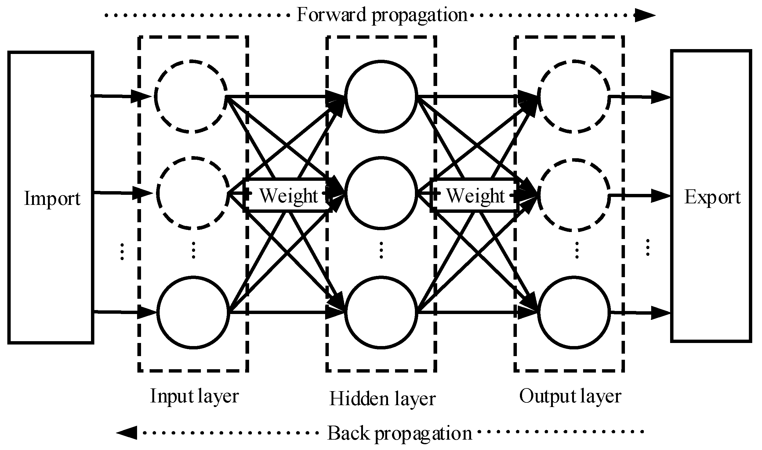
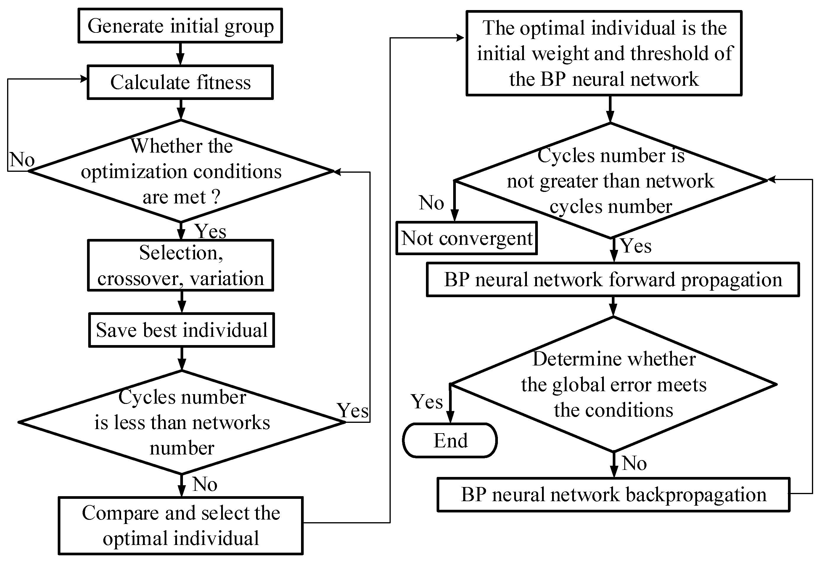
3.1. Optimization of BPNN

Establishing a highly nonlinear mapping relationship between input and output information is the main principle of the BPNN [19]. In Figure 1, the BPNN is mainly divided into three parts. Each layer is connected and communicated through weight connections. The learning of the BPNN mainly includes four steps: pattern forward propagation, error back propagation, memory training, and learning convergence. After setting an input format in advance in the BPNN, it will process and transmit information step by step from the neurons in the input layer to the neurons in the hidden layer, and then to the neurons in the output layer in the order of pattern propagation. Finally, corresponding outputs will be generated in each neuron of the output layer. These outputs produce an output result in the corresponding order. The actual output of the output layer and the expected results are processed. If the error does not meet the preset requirements, error backpropagation is required. The calculated error value is transmitted along the set path in the reverse direction. Appropriate modifications were made to the threshold values of each neuron and the weights of the connections between them to approximate the set target values.
The performance of cloud models is reflected by three parameters: entropy (En), hyperentropy (He), and the expected value (Ex) [20]. In Figure 2, entropy (En) is mainly used to reflect the range size of recognized data values within a concept’s relevant domain. Hyperentropy (He) refers to the entropy corresponding to the concept itself, reflecting the dispersion of each cloud droplet. The expected value Ex is the value that best reflects the performance of the corresponding concept among all data in the universe.
In cloud theory, cloud droplets can randomly tilt in a certain direction when forming a cloud. Applying it to the GA can improve the probability of inheritance and mutation in the GA, reducing the blindness of the traditional GA. Thus, the convergence performance is improved and the operational efficiency of the GA is accelerated. In the cloud GA, the first step is to perform a crossover operation. Formula (1) is a method for exchanging information between chromosomes a m and a n at population k .
a m k = a m k ( 1 b ) + a n k b a n k = a n k ( 1 b ) + a m k b
In Formula (1), b is a random number within range of [0, 1]. The cloud GA determines the probability of the crossover operation p c 1 based on the generation algorithm of conditional cloud Y in Equation (2).
p c 1 = k e ( f E x 1 ) 2 2 ( E n 1 ) 2 , f > f k , f < f
In Formula (2), e is the base of natural logarithm, c 1 is the control coefficient, E x 1 is the expected value, E n 1 represents entropy after random processing, and f is the fitness value of the current operation entity. f represents the average value of individual fitness after updating in Formula (3).
f = j = 1 n f j / n
f j in Formula (3) is the fitness value of individual j after updating. The calculation of the expected value E x 1 in Formula (2) is shown in Formula (4).
E x 1 = f
The calculation of entropy E n 1 in Formula (2) is shown in Formula (5).
E n 1 = ( f max f ) / c 1
In Formula (5), c 1 is the control coefficient, and f max represents the maximum fitness of all individuals. The calculation of super entropy H e 1 is shown in Formula (6).
H e 1 = E n 1 / c 2
In Formula (6), c 2 refers to the control coefficient. E n 1 represents entropy after random processing, and its calculation is shown in Formula (7).
E n 1 = R A N D N ( E n 1 , H e 1 )
The difference between the cloud GA and the traditional GA lies in the way in which probability values of cross-mutation operations are determined. The uncertainty value u was generated based on sample uniformity. Then, a weighted value was used to determine E x 1 for the parent sample, where E n 1 is equal to value obtained by dividing the variable search range by c 1 and H e 1 = E n 1 / c 2 . Finally, the method of generating the conditional cloud Y using cloud theory is used to determine the magnitude of the probability of crossover.
Cross operation in the cloud GA requires mutation operation, and Formula (8) is the method for chromosome l to undergo mutation operation at h .
a l n = a l h + ( a l h a max ) f ( g ) a l h + ( a min a l h ) f ( g )
In Formula (8), a max stands for the upper bound of a l h , and a min represents the lower bound of a l h . Formula (9) is the calculation of f ( g ) .
f ( g ) = r 2 ( 1 g / G max )
In Formula (9), r 2 is the number generated within a set range, g refers to the number of data updates, and G max represents the maximum number of data updates. The specific calculation process for determining mutation operation probability p c 2 by using the cloud GA is shown in Formula (10).
p c 2 = k e ( f E x 2 ) 2 2 ( E n 2 ) 2 , f > f k , f < f
f in Formula (10) is the larger fitness value obtained by an individual after crossover operation. E n 2 represents entropy after random processing in the cross operation. The calculation of the expected value E x 2 in the cross operation is shown in Formula (11).
E x 2 = f
The calculation of entropy E n 2 in the cross operation is shown in Formula (12).
E n 2 = ( f max f ) / c 3
In Formula (12), c 3 also represents the control coefficient. The calculation of hyperentropy H e 2 in the cross operation is shown in Formula (13).
H e 2 = E n 2 / c 4
In Formula (13), c 4 also represents the control coefficient. The calculation of entropy E n 2 after random processing in the cross operation is shown in Formula (14).
E n 2 = R A N D N ( E n 2 , H e 2 )
Taking original individuals E x 2 , E n 2 is equal to the face-changing search range divided by c 3 , H e 2 = E n 2 / c 4 . When certainty u is less than the mutation probability value, so the mutated individual is determined by using cloud theory methods.
Using the cloud GA to optimize the BPNN, the specific process is mainly divided into two types. One is to optimize and improve the initial weight and threshold of the BPNN. The second is to comprehensively improve and optimize the initial weights, thresholds, and overall topological shape of the BPNN. The specific flowchart of optimizing the initial threshold and weight values of the BPNN by using the cloud GA is shown in Figure 3. Firstly, the initial thresholds and weights in the BPNN were classified and sorted. After the sorting was complete, a random data information vector was generated as the population chromosome. According to these chromosomes, the appropriate numerical function of fitness was determined, and the fitness values of all individuals were calculated. According to the fitness result judgment, an appropriate standard value was set for the number of cycle operations. If the set standard met the preset conditions of the cloud GA, then this standard was used as the ideal parameter for the initial weight and threshold of the BPNN. Otherwise, the operation of the GA was followed, and individual updates were iterated until the preset requirements were met. The optimal value obtained by the cloud GA is the reference value for the initial threshold and weight of the BPNN. By following the learning process of the BPNN, global optimization can be completed.
The use of the cloud GA to optimize the topological structure of the BPNN mainly involves optimizing the hidden layer and total number of neurons in the hidden layer of the entire neural network. The specific optimization process is reflected in the encoding of the topological structure. The encoding of topological structures mainly adopts two methods: binary encoding and integer encoding. The encoding of binary encoding is simple and easy to implement, and it is a commonly used method for topological structure encoding. The code sequence is divided into three parts. Code string l represents the total number of layers included in the hidden layer, and β is 0 or 1. The code string l 1 represents the number of neurons contained in the first hidden layer. The code string l 2 represents the number of neurons contained in the second hidden layer. There is a certain conversion relationship between l 1 and l 2 , and their specific conversion is shown in Equation (15). Among them, j represents the length which is taken for encoding the number of neurons in each part of the corresponding hidden layer, which is generally determined based on the actual situations.
l 1 = 2 0 β 11 + 2 1 β 12 + + 2 j 1 β 1 j l 2 = 2 0 β 21 + 2 1 β 22 + + 2 j 1 β 2 j
The optimization of the integer encoding process mainly involves encoding the number of nodes and its neurons as L , l 1 , l 2 in the hidden layer, respectively, and all require encoding using integers within a certain range. Compared with binary encoding, integer encoding has shorter sequences that are limited to a certain range. Therefore, the implementation of this encoding method is relatively complex. Therefore, this study considers using binary encoding to determine the hidden layer number and total number of neurons, as well as optimizing the BPNN’s topological structure.

3.2. DN FD based on BPNN

Most DN systems are composed of multiple subsystems, which are combined in a hand-in-hand manner. The interconnection between these subsystems is mainly achieved through the use of interconnection switches L. As shown in Figure 4, I0 is the circuit breaker and I1, I2, I3, I4 are segmented developments in the DN line. The interconnection switch decomposes the DN into two independent sub grid systems to reduce fault location range. Therefore, when conducting a fault analysis, only one sub grid system needs to be collected and analyzed, which greatly reduces the difficulty of data analysis and processing, thereby improving the efficiency of FD. To use the BPNN for DN FD, an FTU device is first required to collect fault information samples from the DN and establish corresponding fault sample sets. For the collection of sample data, each small area in the power grid will be equipped with an FTU device. FTU devices can compare the current size in each circuit with the preset setting value, and the comparison results are collected to achieve information collection for each circuit in the power grid [21,22]. When there is a difference between the current value and the setting value, the line data information collected by the FTU device is 1. When there is no difference between the current value and the setting value, the information collected by the FTU device is 0. For information data collected by the FTU device after initializing, they can be used as input information for the BPNN. And fault information location can be analyzed based on the BPNN to achieve the fault diagnosis and positioning.
The more complex the distribution system is, the more complex its corresponding power grid topological structure becomes. Traditional BPNNs for FD in a complex DN often suffer from local optima due to slow convergence speed, leading to certain deviations in fault localization and diagnosis [23]. The optimized BPNN can effectively avoid this defect. Like the traditional BPNN, the optimized BPNN requires the collection of fault information before FD. And the BPNN structure can be determined based on the collected data information. The difference is that the initial weight and threshold settings in the optimized BPNN depend on the cloud GA for determination. As shown in Figure 4, assuming a fault occurs at A, switches I 2 , I 3 , and I 0 will generate abnormal current data, while I 3 and I 4 will not flow through the abnormal current. For these current data, the FTU device will collect it and represent it in an ordered vector. These vectors are the input information set of BPNN for FD, and the specific expression is A = ( X 1 , X 2 , , X M ) T . By inputting the collected fault vector information into the BPNN for operation calculation, the fault location A can be identified.

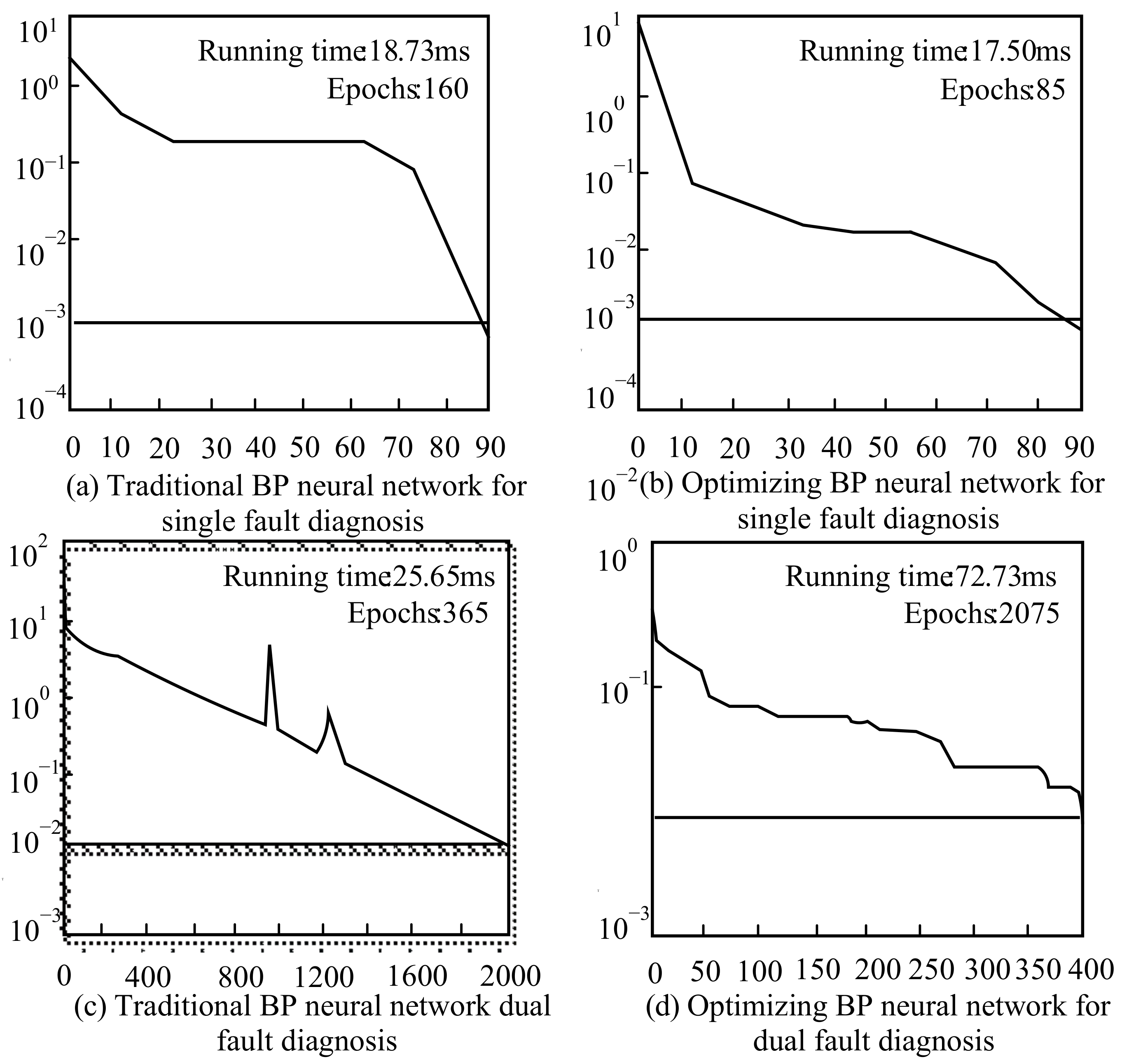
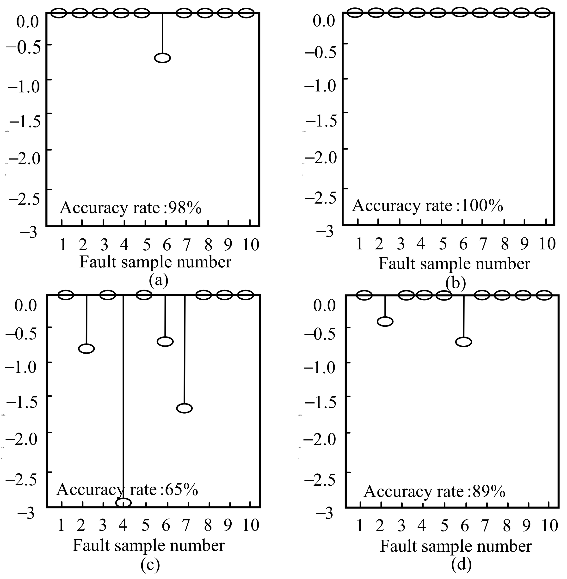
4. Simulation Analysis Based on BPNN Optimization Algorithm

In order to verify whether the improved BP neural network is suitable for fault location in distribution networks, this section will conduct a simulated verification of the effectiveness of the improved BP neural network applied to fault location in distribution networks. In the experiment, the detection performance of fault location methods was compared using indicators such as iteration number, convergence, iteration time, and fault location accuracy. At the same time, different algorithms were applied to the fault location of the same distribution network in the experiment to observe the performance of the improved BP neural network. A distribution network system was set up for online fault location analysis using different methods in this study, as shown in Figure 5.
A partial and small “hand in hand” DN is shown in Figure 5. The diagram includes circuit breaker I0, which is a device used to record the switch information of various DNs. The Figure also includes current information from the FTU numbered I1 to I9, as well as the corresponding X1 to X9 sections. The FTU device is numbered I1-I20, X1-X19 represents each line segment, and I0 represents the circuit breaker.
The improved BPNN mentioned above was used to locate the fault location of the DN. The first step was to establish a learning sample. Data information of each line segment collected by the FTU device were organized and statistically analyzed, and a relevant data sample vector set was established. The vector information of the sample is shown in Table 1. Based on the vector information, the number of neurons that required an input layer was 10. The corresponding number of neurons for the output layer was 10. The number of neurons in the hidden layer was calculated to be 9.
This experiment selected 10 fault samples as the input sample set for the optimized BPNN training, represented by P1, P2, P3, P4, and P5, respectively. Before running the BPNN, the initial population size of the cloud GA was set to 60, the iteration number of the GA was 80, and the optimization goal of the BPNN was set to 0.001. Finally, the traditional BPNN and the optimized BPNN were used to iterate the input fault information set, and the final output results of the optimized BPNN are shown in Table 2. By using the optimized BPNN to locate FDs of five fault samples in the DN, the fault location was determined for each sample set, indicating that the optimized BPNN has a certain effectiveness and stability in the FD of DNs.
The iterative results obtained by two different neural networks are shown in Figure 6. Figure 6a shows the single FD simulation training results of the traditional BPNN. Figure 6b shows the single FD simulation training results of the optimized BPNN. Figure 6c shows the dual FD simulation training results of the traditional BPNN. Figure 6d shows the dual FD simulation training results of the optimized BPNN. By comparing and analyzing Figure 6a,b, when conducting a single FD on the DN, the simulation time of the traditional BPNN is 18.73 ms, and its simulation step number is 160 steps. The simulation time of the optimized BPNN is 17.50 ms, and its simulation step number is 85. The simulation training time difference between the traditional BPNN and the optimized neural network is relatively small. But, the simulation step number used in the optimized BPNN is much smaller than that of the traditional BPNN, indicating a significant improvement in learning speed of the optimized BPNN. By comparing and analyzing Figure 6c,d, when performing the dual FD on the DN, the traditional BPNN operation requires 72.73 ms and the simulation step number is 2075. The optimized BPNN requires 25.65 ms to run and 365 simulation steps. The optimized BPNN spends less time and has fewer simulation steps in the dual FD of the DN than the traditional neural network, while its accuracy is much higher than the traditional BPNN. This is because the traditional genetic algorithms are prone to drawbacks such as poor convergence and local optima. The algorithm dimension is too high, resulting in excessively long iteration convergence time. In comparison, the improved genetic algorithm has the advantages of high fault location rate, low algorithm dimension, and good iterative convergence when dealing with fault location of distribution network lines. Therefore, it can be concluded that the optimized BPNN has high accuracy and efficiency when dealing with dual faults in the DN.
The error statistics of the traditional BPNN and the optimized neural network simulation training results are shown in Figure 7. Figure 7a shows the single FD simulation training error results of the traditional BPNN. Figure 7b shows the single FD simulation training error results of the optimized BPNN. Figure 7c shows the dual FD simulation training error results of the traditional BPNN. Figure 7d shows the dual FD simulation training error results of the optimized BPNN. By comparing and analyzing various graphs, both the traditional and optimized BPNN can achieve an accuracy of over 98% for single fault analysis. When performing dual FD, the accuracy of the traditional BPNN is 65%, while the accuracy of the optimized BPNN reaches 89%. The accuracy of the optimized BPNN for dual FD is significantly higher than the traditional BPNN, and the error margin is also significantly lower. It can be seen that the accuracy of the improved algorithm decreases when it is used for dual fault localization. This is because the increase in the number of faults that need to be located leads to an increase in computational difficulty, resulting in a decrease in the accuracy of the algorithm’s fault location. Therefore, further verification of the application effect of the improved algorithm in multiple faults is needed in subsequent experiments, as shown in Figure 8.
The simulation analysis of multiple fault locations was also carried out in the experiment, and the results of the fitness function of different methods are shown in Figure 8. When lines 5, 7, 11, 13, and 16 fail, the fault location time of the improved algorithm is 158.77 ms, the number of iterations is 75, and the fitness value is 1.0. The fault location time and fitness of this method are lower than those of other methods. This indicates that the improved algorithm has the advantages of fast iteration speed, high fault localization rate, and low algorithm dimension when dealing with multiple fault localization. The results show that the introduction of the cloud genetic algorithm effectively improves the accuracy and operational efficiency of the BP neural network in multiple fault localization.
To conduct a more comprehensive evaluation of the improved algorithm mentioned above, relevant data statistics were also conducted in the experimental validation, and the receiver operating characteristic (ROC) curves of different methods were plotted. This curve uses specificity as the horizontal axis and sensitivity as the vertical axis. It can demonstrate the performance of various methods. When the area under the ROC curve is large, the algorithm performance is better. The comparison results between the optimized BPNN and the ROC of references [24,25,26,27] are shown in Figure 9. From the graph, the improved algorithm proposed in the experiment has a larger area under the curve, indicating that this method has better overall performance. From the enlarged images of some curves, the improved method proposed in the experiment has a slightly fluctuating ROC curve, but overall it is relatively smooth. However, another comparison method, when magnified, shows greater volatility. This is because the cloud genetic algorithm is a globally applicable and robust search optimization method. It can effectively improve the convergence speed of the BP neural network and prevent the network from falling into local minimum points. The optimized BP neural network has higher learning efficiency, stability, and robustness.

5. Conclusions

Electric energy is one of the important energy sources required for various technological production and people’s happy lives. Therefore, studying the DN and achieving safe and effective management of the DN is the research goal of many researchers. The fault detection methods for power grids include various methods [28]. Researchers have conducted a large number of experiments to establish detection methods for different power grid faults [29]. Research has shown that BP neural networks have good application effects in fault detection [10]. However, traditional BP neural networks have poor convergence in practical applications and are prone to falling into local optima. In terms of improving the convergence speed of BP neural networks, general optimization algorithms have made certain improvements [15]. However, the optimized BP neural network still has problems such as being prone to falling into local optima, oscillation and poor robustness due to the improvement of learning rate, and the sensitivity of network performance to the initial values of the network. The cloud genetic algorithm is a globally applicable and robust search optimization method. It can effectively improve the convergence speed of the BP neural network and prevent the network from falling into local minimum points [17]. This study investigates the application of the BPNN in FD positioning in the DN. And, on the basis of the traditional BPNN, the GA and cloud theory were introduced to achieve the optimization of the traditional BPNN. Finally, the optimized BPNN algorithm is applied to diagnosis and location analysis of single and dual faults in the DN, and the simulation training results of the traditional BPNN and the optimized BPNN were compared. The results show that the operation of the optimized BPNN requires 25.65 ms and the simulation steps are 365. The optimized BPNN has high effectiveness, stability, and accuracy in FD localization. In the diagnosis and positioning of dual faults, the optimized BPNN exhibits a higher FD rate, with an accuracy of 89%, and its FD localization speed is much higher than the traditional BPNN. In the comparison of ROC curves, the optimized BPNN has a larger area under the curve and has a smoother curve. Although research results show that the optimized method has good performance, this model requires many samples for learning. This leads to certain limitations in the optimized method in practical applications. In addition, the local optimal solution problem has not yet been fundamentally solved. Therefore, further in-depth research is needed to diagnose and locate multiple faults in the DN.

Author Contributions

Formal analysis, C.Z., Y.L., J.M. and H.W.; data curation, S.G., Y.L., J.M. and H.W.; writing—original draft preparation, C.Z. and S.G.; writing—review and editing, C.Z. and S.G. All authors have read and agreed to the published version of the manuscript.

Funding

This work was supported by The National Key Research and Development Program of China (2020YFC0833400).

Data Availability Statement

The data presented in this study are available on request from the corresponding author.

Conflicts of Interest

The authors declare no conflict of interest.

References

  1. Hichri, A.; Hajji, M.; Mansouri, M.; Harkat, M.F.; Nounou, M. Fault Detection and Diagnosis in Grid-Connected Photovoltaic Systems. In Proceedings of the 2020 17th International Multi-Conference on Systems, Signals & Devices (SSD), Monastir, Tunisia, 20–23 July 2020; pp. 201–206. [Google Scholar]
  2. Kemikem, D.; Boudour, M.; Benabid, R.; Tehrani, K. Quantitative and Qualitative Reliability Assessment of Reparable Electrical Power Supply Systems using Fault Tree Method and Importance Factors. In Proceedings of the 2018 13th Annual Conference on System of Systems Engineering (SoSE), Paris, France, 19–22 June 2018; pp. 452–458. [Google Scholar]
  3. Afrasiabi, S.; Afrasiabi, M.; Jarrahi, M.A.; Mohammadi, M. Fault location and faulty line selection in transmission networks: Application of improved gated recurrent unit. IEEE Syst. J. 2022, 16, 5056–5066. [Google Scholar]
  4. El Mrabet, Z.; Sugunaraj, N.; Ranganathan, P.; Abhyankar, S. Random forest regressor-based approach for detecting fault location and duration in power systems. Sensors 2022, 22, 458. [Google Scholar]
  5. Wei, M.; Hu, X.; Yuan, H. Residual displacement estimation of the bilinear SDOF systems under the near-fault ground motions using the BP neural network. Adv. Struct. Eng. 2022, 25, 552–571. [Google Scholar]
  6. Cruz, J.D.L.; Ali, M.; Vasquez, J.C.; Guerrero, J.M.; Su, M.A. Fault location for distribution smart grids: Literature overview, challenges, solutions, and future trends. Energies 2023, 16, 2280–2316. [Google Scholar]
  7. Rocha, S.A.; Mattos, T.G.; Cardoso, R.T.; Silveira, E.G. Applying artificial neural networks and nonlinear optimization techniques to fault location in transmission lines—Statistical analysis. Energies 2022, 15, 4095. [Google Scholar]
  8. Sahoo, B.K.; Pradhan, S.; Panigrahi, B.K.; Biswal, B.; Patel, N.C.; Das, S. Fault Detection in Electrical Power Transmission System using Artificial Neural Network. In Proceedings of the International Conference on Computational Intelligence for Smart Power System and Sustainable Energy (CISPSSE), Keonjhar, India, 29–31 July 2020; pp. 1–4. [Google Scholar]
  9. Li, M.; Chen, Z.; Dong, J.; Xiong, K.; Chen, C.; Rao, M.; Peng, J. A data-driven fault diagnosis method for solid oxide fuel cell systems. Energies 2022, 15, 2556. [Google Scholar]
  10. Xiao, M.; Liao, Y.; Bartos, P.; Filip, M.; Geng, G.; Jiang, Z. Fault diagnosis of rolling bearing based on back propagation neural network optimized by cuckoo search algorithm. Multimedia tools and applications. Multimed. Tools Appl. 2022, 81, 1567–1587. [Google Scholar]
  11. Zhao, Y.; Du, W.; Wang, Y. Study on intelligent shape finding for tree-like structures based on BP neural network algorithm. J. Build. Struct. 2022, 43, 77–85. [Google Scholar]
  12. Xiao, M.; Zhang, W.; Zhao, Y.; Xu, X.; Zhou, S. Fault diagnosis of gearbox based on wavelet packet transform and CLSPSO-BP. Multimed. Tools Appl. 2022, 81, 11519–11535. [Google Scholar]
  13. Zhang, X.; Jiang, S. Study on the application of BP neural network optimized based on various optimization algorithms in storm surge prediction. Proc. Inst. Mech. Eng. Part M J. Eng. Marit. Environ. 2022, 236, 539–552. [Google Scholar]
  14. Li, T.; Yin, Y.; Yang, B.; Hou, J.; Zhou, K. A self-learning bee colony and GA hybrid for cloud manufacturing services. Computing 2022, 104, 1977–2003. [Google Scholar]
  15. Wen, X.; Sun, Q.; Li, W.; Ding, G.; Song, C.; Zhang, J. Localization of low velocity impacts on CFRP laminates based on FBG sensors and BP neural networks. Mech. Adv. Mater. Struct. 2022, 29, 5478–5487. [Google Scholar]
  16. Fu, Y.; Liu, Y.; Yang, Y. Multi-sensor GA-BP algorithm based gearbox fault diagnosis. Appl. Sci. 2022, 12, 3106. [Google Scholar]
  17. Xia, X.; Qiu, H.; Xu, X.; Zhang, Y. Multi-objective workflow scheduling based on GA in cloud environment. Inf. Sci. 2022, 606, 38–59. [Google Scholar]
  18. Materwala, H.; Ismail, L.; Shubair, R.M.; Buyya, R. Energy-SLA-aware GA for edge–cloud integrated computation offloading in vehicular networks. Future Gener. Comput. Syst. 2022, 135, 205–222. [Google Scholar]
  19. Li, S.; Fan, Z. Evaluation of urban green space landscape planning scheme based on PSO-BP neural network model. Alex. Eng. J. 2022, 61, 7141–7153. [Google Scholar]
  20. Zhu, J.; Chen, H.; Pan, P. A novel rate control algorithm for low latency video coding base on mobile edge cloud computing. Comput. Commun. 2022, 187, 134–143. [Google Scholar]
  21. Maghami, M.R.; Pasupuleti, J.; Ling, C.M.; Li, M.S. Impact of photovoltaic penetration on medium voltage distribution network. Sustainability 2023, 15, 5613. [Google Scholar]
  22. Xiong, G.; Yuan, X.; Mohamed, A.W.; Chen, J.; Zhang, J. Improved binary gaining–sharing knowledge-based algorithm with mutation for fault section location in DNs. J. Comput. Des. Eng. 2022, 9, 393–405. [Google Scholar]
  23. Hu, K.; Wang, L.; Li, W.; Cao, S.; Shen, Y. Forecasting of solar radiation in photovoltaic power station based on ground-based cloud images and BP neural network. IET Gener. Transm. Distrib. 2022, 16, 333–350. [Google Scholar]
  24. Hong, Q.B. Improved fault location method for AT traction power network based on EMU load test. Railw. Eng. Sci. 2022, 30, 532–540. [Google Scholar]
  25. Awasthi, S.; Singh, G.; Ahamad, N. Identification of type of a fault in distribution system using shallow neural network with distributed generation. Energy Eng. 2023, 120, 811–829. [Google Scholar]
  26. Azeroual, M.; Boujoudar, Y.; Aljarbouh, A.; Moussaoui, H.E.; Markhi, H.E. A multi-agent-based for fault location in DNs with wind power generator. Wind. Eng. 2022, 46, 700–711. [Google Scholar]
  27. Yuan, R.; Lv, Y.; Lu, Z.; Li, S.; Li, H. Robust fault diagnosis of rolling bearing via phase space reconstruction of intrinsic mode functions and neural network under various operating conditions. Struct. Health Monit. 2023, 22, 846–864. [Google Scholar]
  28. Kaplan, H.; Tehrani, K.; Jamshidi, M. Fault diagnosis of smart grids based on deep learning approach. In Proceedings of the 2021 World Automation Congress (WAC), Taipei, Taiwan, 1–5 August 2021; pp. 164–169. [Google Scholar]
  29. Dogra, R.; Rajpurohit, B.S.; Tummuru, N.R.; Marinova, I.; Mateev, V. Fault detection scheme for grid-connected PV based multi-terminal DC microgrid. In Proceedings of the 2020 21st National Power Systems Conference (NPSC), Gandhinagar, India, 17–19 December 2020; pp. 1–6. [Google Scholar]
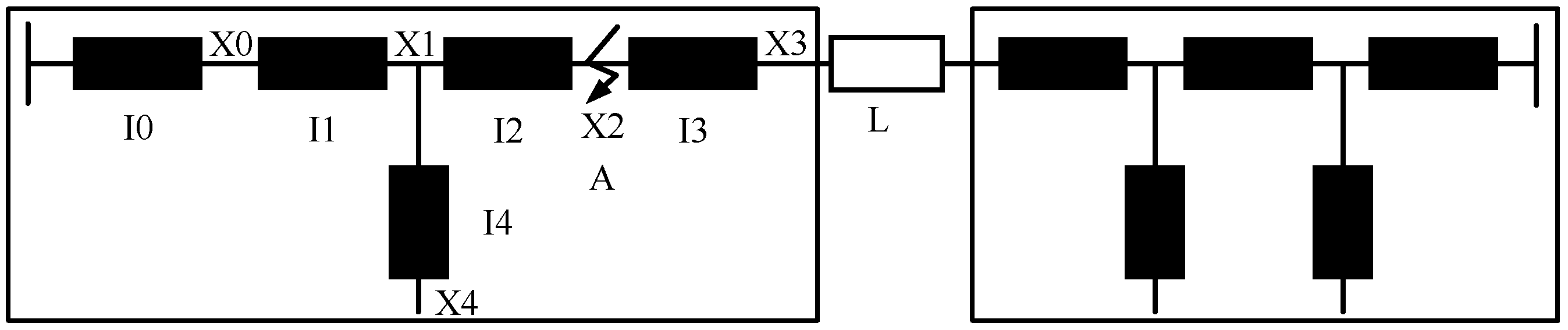
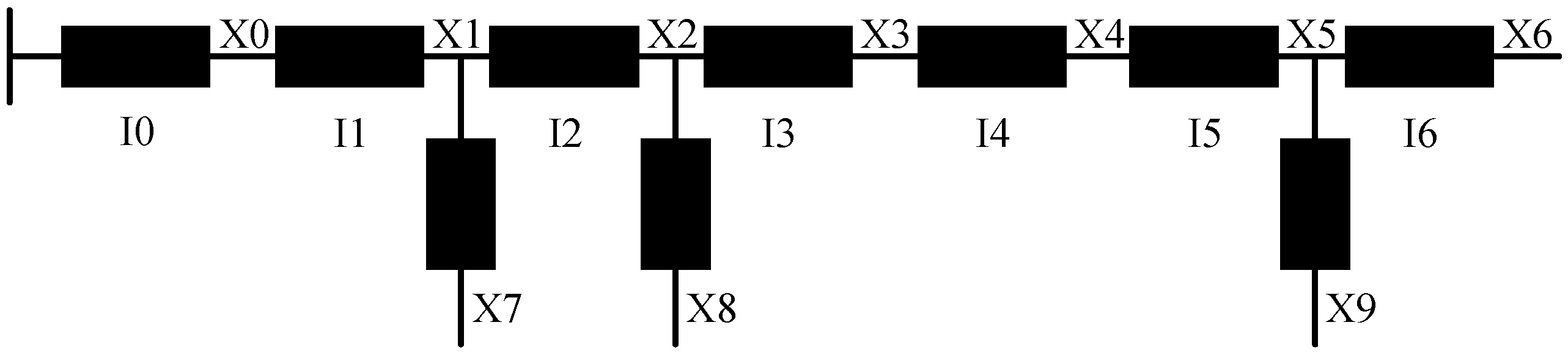
Figure 1. BPNN structure diagram.
Processes 11 01947 g001
Figure 2. Characteristic parameters of the cloud model.
Processes 11 01947 g002
Figure 3. Operation process of the BPNN cloud genetic optimization algorithm.
Processes 11 01947 g003
Figure 4. Hand-in-hand DN.
Processes 11 01947 g004
Figure 5. Schematic diagram of DN.
Processes 11 01947 g005
Figure 6. Iterative training results of the BPNNFD.
Processes 11 01947 g006
Figure 7. Analysis chart of error results. (a) shows the single FD simulation training error results of the traditional BPNN. (b) shows the single FD simulation training error results of the optimized BPNN. (c) shows the dual FD simulation training error results of the traditional BPNN. (d) shows the dual FD simulation training error results of the optimized BPNN.
Processes 11 01947 g007
Figure 8. Fitness. (Maghami et al. 2023 [21], Xiong et al. 2022 [22], Hu et al. 2022 [23], Hong 2022 [24]).
Processes 11 01947 g008
Figure 9. ROC curve. (Maghami et al. 2023 [21], Xiong et al. 2022 [22], Hu et al. 2022 [23], Hong 2022 [24]).
Processes 11 01947 g009
Table 1. Input vector and output vector of fault sample set.
VectorFTU1234567891011
Input vectorI001111111111
I100111111111
I200011111111
I300001111111
I400000111111
I500000011111
I600000001111
I700000000111
I800000000011
I900000000001
Output vectorI001000000000
I100100000000
I200010000000
I300001000000
I400000100000
I500000010000
I600000001000
I700000000100
I800000000010
I900000000001
Table 2. Output results of the optimizing BPNN.
P1P2P3P4P5
X00.00210.00280.00310.00300.0019
X10.00230.00130.00570.00070.9901
X20.00160.00220.00100.89990.0029
X30.99160.00280.00460.00550.0012
X40.00250.00290.00120.00110.0023
X50.00180.00010.99160.00210.0033
X60.00210.99170.00250.00390.0053
X70.00260.00360.00180.00390.0011
X80.00260.00580.00210.00120.9965
X90.00020.00130.00360.00070.0009
Fault pointX3X6X5X2X8
Disclaimer/Publisher’s Note: The statements, opinions and data contained in all publications are solely those of the individual author(s) and contributor(s) and not of MDPI and/or the editor(s). MDPI and/or the editor(s) disclaim responsibility for any injury to people or property resulting from any ideas, methods, instructions or products referred to in the content.

