1. Introduction
The investment goal of a pension fund has special features when compared to other institutional investors. These features stem from the pre-determined liabilities that a pension fund has to meet under a defined contribution (DC) scheme, a defined benefit (DB) scheme, or a mixture of both. For example, in a typical DB scheme, each pension’s member contributes periodically to the fund, which invests the contributions to the risky market, aiming to meet the promised liability at the time of retirement. In principle, this creates an optimization problem with random dynamic endowment and a terminal payment (random or not).
In a similar context, we take the position of a pension fund for which the pension payments are given by a pre-determined function of the members’ contributions. The latter are set as a proportion of the wage process, which is possibly correlated to the market the pension fund invests in. Our initial question is whether the pension fund could guarantee the promised liability to the members, or, alternatively, what is the distance between the current capital and the promised payment. For this, we consider the pension payment as a path-dependent derivative security whose underlying asset is the members’ wage (stochastic) process. Since the wage process is neither tradeable nor replicable, the valuation using solely the non-arbitrage assumption is not enough (the market is incomplete). Therefore, we propose as a measure of distance to liability full-hedging the so-called super-hedging price, i.e., the minimum cost of the portfolio whose value at the time of retirement is higher than or equal to the liability.
1.1. Contributions
The idea of considering a pension’s fund liability as a derivative payoff is not new in the literature (e.g.,
de Jong 2008). Assuming the market’s completeness yields a single price of the liability (as the discounted expectation under the unique risk-neutral measure) and, hence, there is an admissible portfolio that replicates the liability almost surely (as in
Sundaresan and Zapatero 1997). However, markets are definitely not complete. In particular, the wage process, which both finances the pension plan and determines the pension’s liability, is normally neither tradeable nor replicable. Rather, it is an untradeable process that can be very closely related to the investment universe of a pension fund. In other words, a model that imposes a complete market surely underestimates the risk that a pension fund faces, since the undertaken risk is considered hedgeable although it is not.
On the other hand, market incompleteness makes the valuation of a pension plan rather subjective. Namely, the non-arbitrage pricing method does not give a single price (but an interval of prices) and hence, a single valuation needs some subjective criterion and/or estimations, for example, pricing with expectation (under subjective probability measure), increased by a risk premium (also adapted to subjective risk preferences) or a pricing that is based on the market’s competition. While all these methods are valid and meaningful, their connection to the subjectivity is strong. On the contrary, risk metrics that are less dependent on subjective beliefs (probability measure and risk preferences) are occasionally more appropriate and indicative.
The super-hedging value is the upper bound of the non-arbitrage pricing interval, which does not depend on either the subjectivity of beliefs or the risk preferences.
1 We consider it as the minimum capital that the pension fund manager needs in order to cover the liability at the retirement date (with probability one). In other words, this metric can be seen as an upper bound of the amount of cash that suffices to guarantee the solvency of a DB plan and hence, its difference from the current value of the pension fund’s assets can be used as a distance measure to fully hedged liability.
2One problem with the use of a super-hedging value as an indicative pension’s plan valuation is that in the classical diffusion continuous-time models, it can be unbounded.
3 For this reason, our goal is to examine how indicative this valuation is in the
simplest possible incomplete market model for which we are able to calculate explicit formulas and figure out the effects of all parameters. Namely, we consider a discrete-time model with a single risky asset and a stochastic wage process, where at each period there are only three possible events, i.e., a trinomial model (in the spirit of the classical multi-period binomial model of
Cox et al. (
1979)). In contrast to the binomial model, here the market is incomplete. As we will see in the sequel, this model is both simple and rich enough to include all the important features of the valuation, such as the volatility of the wages and the market, their relation, the flexibility of contribution rate, the form of the pension’s liability, etc. We argue that, as the binomial model is so useful for non-arbitrage pricing, the simple trinomial model is similarly useful for the pension plan’s valuation.
Through the explicit solution of the super-hedging value in the trinomial model we first verify its meaningfulness (in contrast to the classical diffusion model). In addition, we obtain that it is decreasing with respect to the contribution and increasing with respect to the liability (as expected). The size of the super-hedging value is affected only by the unhedgeable part of the wage process. More precisely, the extra event at each step (which makes the wage unhedgeable) affects the super-hedging value only when it gives a higher wage than the hedgeable part of the wage process. Furthermore, the effect of the relation between the wage and the risky asset on the super-hedging value appears in a rather simple form. In particular, a negative relation increases the value when the range of a risky asset is sufficiently high. Putting it in a simple phrase, a negative relation tends to increase the super-hedging value if the risky asset has high volatility. On the other hand, when the unhedgeable part of the wage process is too high, this relation does not affect the value (since it is hedged out).
As for the super-hedging investment strategy, we first obtain that, as long as the unhedgeable part of the wage is not very high, a positive (resp., negative) relation between the wage and the risky asset results in a positive (resp., negative) position in the risky asset. However, even when the relationship is positive, in the case where the unhedgeable part of the wage is sufficiently high, the super-hedging strategy indicates a short position in the risky asset. Besides this result, a higher liability (resp., contributions) implies a higher (resp., lower) investment (in absolute value) in the risky asset. The standard monotonicity between the volatility (i.e., the range) of the risky asset and the investment position also holds.
It is quite usual in the pension fund industry for managers to charge a performance fee (see, for instance,
Deelstra et al. (
2003),
Giacinto et al. (
2011),
Sundaresan and Zapatero (
1997) and
Wang et al. (
2018)). This creates an extra motive to achieve a better performance, even when the fund does have the cash to super-hedge the undertaken liability. In fact, pension fund managers normally impose their subjective beliefs about the probability of future outcomes and use personalized risk preferences together with the pension’s liability to form “optimal” investment strategies.
However, how could these strategies differ from the super-hedging strategy in the cases where the full hedging of the liability is feasible? In other words, our next exercise is to apply widely-used optimization investment strategies in our setting and emphasize the induced differences (in sign and size) to the objective super-hedging strategy.
For this, we follow the related literature and model a pension fund’s subjective investment criterion under a utility maximization problem on the wealth surplus (i.e., the difference between the portfolio value and the liability payment). In short, we emphasize that such optimization objectives can heavily deviate from the super-hedging value both in size and sign. Through a numerical exercise, we show that a super-hedging investment can be relatively small, while the “optimal” investment can take very large positions (especially under CRRA preferences). In other words, even if the pension fund has the capital to super-hedge the liability, an investment goal that focuses on the wealth surplus can lead to a portfolio with much higher risk than needed.
Finally, we consider the case of a potential early exit from the fund. More precisely, we consider a mandatory scheme in the sense that the member does not have the choice to leave, but the early exit occurs randomly at each period (due to death or job termination). The issue that we address in that section is the conditions under which the possibility of an early exit increases the super-hedging valuation. Upon imposing a couple of reasonable assumptions, we obtain that a higher contribution rate implies that an early exit increases the super-hedging value and hence the risk undertaken by the pension fund.
1.2. Connection with the Literature
There exists a considerable body of literature on pension funds that studies the valuation of pension liabilities assuming market completeness. A quite large number of papers models not only pension plans’ valuation, but also the “optimal” asset allocation of a pension fund (in both complete and incomplete markets). Our work is mainly linked to these two literature strands: the valuation of pension liabilities and optimal liability driven investment (LDI) with dynamic stochastic contributions and path-dependent payments.
The super-hedging price is a well-known valuation generally used for pricing contingent claims in incomplete markets. A classical reference in a diffusion market model is
Karoui and Quenez (
1995), where the super-hedging price is defined as the smallest initial capital that allows the sellers to construct a portfolio that dominates the payoff process of an option (see also
Blanchard and Carassus 2022;
Cvitanic et al. 1998). For the wage-indexed liability of a pension fund, the notion of the super-hedging valuation (among several other methods) has been discussed in
de Jong (
2008), where it is mentioned that the super-hedging portfolio is not feasible because of the unbounded wage process. To the best of our knowledge, this is the first time a super-hedging valuation has been applied to a pension plan. Thanks to the tractability of the model, we are also able to obtain indicative insights.
Measuring the distance to the full hedging of liability using an objective notion as the super-hedging valuation is quite novel. The standard measure that is used for a pension fund’s solvency is the funding ratio, which is simply the market value of the assets divided by the present value of future liabilities. A higher funding ratio means a lower underfunding risk (see, for example,
Leibowitz et al. 1994, where the funding ratio is referred to as a universal measure for asset/liability management). In such a measurement, the discounted factor is a subjective parameter that reflects the views of the future expected outcomes and the riskiness of the financial market (see
Bogentoft et al. (
2001),
Bolla et al. (
2016),
Dyachenko et al. (
2022) and
Josa-Fombellida et al. (
2018) for investment strategies based on the funding ratio). While the subjectivity of a measure and the related investment strategies give flexibility to the asset manager, these measures do not necessarily take into account the possibility of full hedging.
On the other hand, there is also a large academic literature that focuses on the optimal investment problem. The approach that is mostly used is the maximization of expected utility under a continuous-time model (applying Merton’s portfolio
Merton (
1971) for a pension fund’s special case as in
Blake (
1998)). One of the related papers that is closer to our approach is
Sundaresan and Zapatero (
1997). It considers a complete continuous-time model and the optimal portfolio is the one that maximizes the expected growth rate of the surplus (the difference between the market value of the assets and the value of the pension liabilities). In the same spirit,
Boulier et al. (
2001) used the surplus over a guaranteed payment, while a more general analytical solution to the dynamic-multiperiod portfolio problem of an investor with risky liabilities and time-varying investment opportunities is developed in
Giamouridis et al. (
2017). In
Lichtenstern and Zagst (
2022), a continuous-time post-retirement optimization problem for a specific plan is solved, which, however, does not allow guarantees. Another widely-used criterion is linked with mean–variance (M-V) preferences (also supported by empirical evidence provided by
Chiu and Wong (
2014) and
Zhou and Li (
2000)). For example,
Menoncin and Vigna (
2017) and
Vigna (
2014) use an M-V criterion considering the difference between the final wealth and an appropriate level of risk/reward (based on
Vigna (
2014)). Note that valuing the pension plans through a utility-maximization problem in these models is both challenging and quite subjective.
There are several optimal management criteria for a pension fund, besides utility maximization, that have been studied. For example,
Siegman (
2007) argues that the typical objectives of pension funds are the minimization of contributions, maximization of pension indexation and minimization of risk with respect to funding (similarly to
Josa-Fombellida and Zapatero (
2008)). On the other hand,
Battochio and Menoncin (
2011) and
Haberman and Sung (
1994) deal with different types of risks related to stability, such as the contribution rate, solvency, salary and inflation risks. In
Hainaut and Deelstra (
2011), an incomplete market is also considered (stochastic wage process) and the objective is the optimization of contribution adjustments and the terminal surplus. An alternative approach is taken in
Haberman and Vigna (
2002), where the periodic optimization goal is to minimize the deviation between the fund’s target and an independent liability process.
Another part of the literature on the optimal investment criteria for DC pension funds focuses on members’ optimal control between consumption and investment during the working life. The general goal is to secure a target level of income that maintains the individual’s pre-retirement lifestyle (see
Kobor and Muralidhar 2020). The seminal papers on that issue (such as
Bodie and Crane (
1997) and
Bodie et al. (
2004)) are reviewed by Bodie et al. in
Bodie et al. (
2010) (where human capital is a highlighted factor). These theoretical studies are consistent with the recent empirical evidence such as that provided in
Azoulay et al. (
2016) and
Gabudean et al. (
2021).
1.3. Structure of the Paper
The remainder of this paper is organized as follows. In
Section 2, we present the model characteristics, describe the idea of super-hedging valuation and state and discuss the main results.
Section 3 is dedicated to the utility-maximization approach and to an indicative numerical exercise.
Section 4 deals with the possibility of an early exit, whereas in
Section 5 we conclude, and in
Appendix A we provide the proofs of the paper’s propositions.
2. Our Model
As already mentioned, we consider a discrete time and space model with a given terminal time that shall be referred to as the
retirement time. We define the set of times
for some
and consider a single (representative) member of a pension fund that gives (stochastic) contributions to the fund at each time in
.
4We adapt a dynamic trinomial model (also used in
Mark 2000), where at each time in
T there are three possible outcomes and a probability measure
that assigns positive probabilities for all three states at each point in time.
5 In particular, there are two stochastic processes: the member’s contribution to the fund and the price of the risky asset (that the pension fund invests in). We let
be the price of a risky asset and
the wage process of the member (a fraction of which is given to the fund as a contribution).
6Regarding the pension payment by the fund to the member at the retirement time, we consider a DB scheme (typical for the first pillar), according to which the fund’s liability is a random lump-sum payment
that depends on the pension member’s wages, i.e.,
. In view of the standard payment functions of the public pension systems (see, among others,
Blake et al. (
2013),
Sundaresan and Zapatero (
1997) and
Wang et al. (
2018)), we impose a linear function of the member’s wages:
where
and
is a pre-determined collection of positive constants called
liability factors. Typically,
increases through time, although this is not necessarily imposed here.
The funding source of the pension plan stems from the member’s contributions, denoted by the stochastic process
. As mentioned above,
is given as a known proportion of the wage process, that is,
where
for each period
.
Our first task is to study how the “promised” pension payment could be valued, or, in other words, how much capital is needed in order to meet the liability. This is an important issue, since a proper valuation indicates whether and to what extent the fund’s existing and expected wealth is sufficient to guarantee the undertaken liability. The setting is the following: The pension fund receives periodic contributions from the member and invests them in the risky and the riskless asset in order to increase the expected return and take advantage of the possible correlation between contributions and wages. Under that perspective, the payoff
can be seen as a path-dependent derivative security and its seller (i.e., the pension fund) obtains its price periodically through the contributions. One could then argue that a way to value the liability (or to measure the needed capital to meet it) is the cost of the replicating portfolio. However, the wage process that generates the liability is non-replicable. The problem could have been solved using non-arbitrage pricing if the market were complete (as in
Sundaresan and Zapatero 1997), but, under market incompleteness, the non-arbitrage pricing does not give a unique price for the liability.
On the other hand, another reasonable way to value such a derivative is by applying a linear pricing kernel and potentially adding a risk premium that stems from a risk-preference function. Although reasonable, this approach has two important disadvantages: it is heavily subjective and underestimates the extreme events. In particular, the probability measure be used to calculate the expected payoff reflects the subjective beliefs of the pension fund, while the risk preferences reflect the risk aversion of the fund. Moreover, valuing with a kernel and a premium provides a valuation such that, even if it is above the current capital of the pension fund, the probability of being insolvent could remain positive.
We propose a less-subjective and conservative approach by applying the notion of the super-hedging price, which is based on the second fundamental theorem of asset pricing (see, for example,
Delbaen and Schachermayer 2005). More precisely, a super-hedging portfolio is a portfolio whose value at time
N is higher than
a.s. and the super-hedging value is the lowest cost at which a super-hedging portfolio can be created (see
Cvitanic et al. (
1998),
de Jong (
2008) and
Karoui and Quenez (
1995) for the use of this notion in a diffusion-market model). In other words, we argue that a meaningful value of a DB pension payment is the lowest cost that the fund should have today to create an investment portfolio that will be a.s. higher than the liability at the retirement.
While, in principle, the super-hedging value is relatively high (it yields a conservative pricing rule), it could provide very interesting indications not only about the solvency of the pension fund, but also regarding the importance of the correlation between the market and the contribution. As mentioned in the introductory section, the super-hedging valuation gives the upper bound of the sufficient amount of capital (cost) in order to meet the liability and, hence, it can be seen as a measure to certain solvency or to full hedging. Furthermore, we could examine how the aforementioned correlation should be taken into account for the investment strategy (in the spirit of an LDI) and whether and to what extent it could reduce the cost of super-hedging. Note also that this exercise is rather objective (within our model setting), which means that its findings are invariant with respect to probability and risk measures.
2.1. Super-Hedging Value and Portfolio
Market incompleteness is equivalent to the non-uniqueness of the risk-neutral probability measures, and the super-hedging value is also equivalent to the supremum of the discounted payoff under the set of all risk-neutral probability measures (see
Delbaen and Schachermayer 2005). Therefore, we first need to characterize the set of risk-neutral measures. The process of the risky asset’s price
satisfies the recursive formula
, for each
, where
is the initial price and the factor
takes the form
The pension fund also invests in a riskless asset whose return each period of time is equal to an interest rate
. In the view of the first fundamental theorem of asset pricing, we make the following standing assumption that guarantees the absence of arbitrage opportunities:
7Similarly to the risky asset price process, we set that the wage process satisfies , ∀, where is the initial wage and the factor equals when the wage increases (at the good or bad state of the risky asset), when the wage decreases (at the good or the bad state) and in the medium state (it can be higher or lower than and ). Note that the wage is not a tradeable asset, which means that there is no specific required inequality for factors , and . Herein, we only assume and that in the medium state the wage factor is .
The set of equivalent risk-neutral probability measures is defined as
In words,
is the set of all equivalent probability measures that make the discounted price process of the risky asset a martingale. The following notation is also useful:
Since the factors are assumed constant through time, simple calculations yield that
is parametrized (with a slight abuse of notation) in the following way:
where
,
and
.
Then, for every random payoff
measureable with respect to the information up to time
N, its initial values that keep the non-arbitrage assumption are given by the interval
The upper bound of the interval above determines the super-hedging value, in the sense that when every price is equal to or higher than that, it creates an arbitrage opportunity. Now, placing the pension lump-sum payment
in the position of
above, we may argue that if the present value of the pension’s fund wealth is higher than
, there is an investment strategy that yields a terminal a.s. equal to or higher than
. Under that perspective, the super-hedging value is the minimum capital (cost) that the fund needs at time zero to create a portfolio that guarantees the payoff of the pension obligation
.
We distinguish two cases according to whether the relation between the wages and the risky asset is positive or negative.
Case 1 (positive relation). Wage increases at the good state by .
Case 2 (negative relation). Wage decreases at the good state by .
Remark 1. Note that the relation (positive or negative) defined above is not directly linked to the linear correlation coefficient. In other words, a positive relation does not necessarily imply a positive correlation, nor does a negative correlation imply a negative relation.
We also set the variables
where
is the complete-market expected wage factor in the case of a positive relation and
in the negative case. In fact,
and
are used to describe the case of a complete market where there are only two possible future states at each node. It would be useful to roughly interpret
as the cost of the hedgeable part of the wage process and the medium state as the unhedgeable part (in the sense that the vanishing of the medium state results in a complete market). We also define the variable
and use the following notation:
Proposition 1. - (i)
The super-hedging value of a pension plan of the form (1) equalswhere . - (ii)
The corresponding super-hedging strategy is given bywhere is defined in (8).
Note that if , i.e., or is higher than , the cost of the hedgeable part of the wage remains higher than the wage at the medium state (in fact, the distance is increasing with respect to the range ). This implies that the super-hedging strategy always has to cover the complete-market expected wage and hence, neither the strategy nor the super-hedging value is affected by the exact level of the factor of the medium state . On the other hand, when , the medium state yields the higher wage and then both the portfolio and the value stem solely from the medium-state wage. In particular, when the medium state gives a higher wage than the hedgeable part of the wage, the super-hedging value is independent of and for both Cases 1 and 2. We summarize this insightful note below.
Corollary 1. - (i)
If , then is not a function of .
- (ii)
If , then is not a function of .
It is important to note that the sign of the sum determines whether the future contributions are sufficient to cover the undertaken liability. If the sum is positive, there is an unhedgeble risk for the pension fund, the value of which can be estimated by the super-hedging value. On the other hand, a negative sum implies that the pension fund can almost surely cover its liability and keep some surplus too. Under a member’s perspective, only a positive sum (i.e., a positive super-hedging value) gives an incentive to participate in this pension plan. Although we consider herein a mandatory participation in the pension plan (first pillar), we state the following assumption that will be imposed in some place in the sequel.
This assumption means that the sum of the weighted difference between factor
and the contribution rate is positive. While for the first years factor
is normally low (even zero, as in our numerical exercise in
Section 3.1), for the years close to the retirement time, its size should be at least equal to the contribution rate. Otherwise, the member has no incentive to participate.
Under Assumption 1, the super-hedging value (considered as the minimum required capital to replicate) is indeed decreasing with respect to the contribution and increasing with respect to the liability. Note that the effect of the relation between the wage and the risky asset on the super-hedging value is clear in (
9). In particular, a negative relation increases the value when
. That is, a negative relation tends to increase the minimum cost of liability replication if the risky asset has high volatility. On the other hand, when the unhedgeable part of the wage price is too high, this relation does not affect the super-hedging value (since it is hedged out).
A direct implication of Assumption 1 is that the sign of the super-hedging strategy (
10) solely depends on the sign of
for each period. In particular, when
is the highest factor of wage change, then the super-hedging strategy indicates a negative position to the risky asset. Hence, when Case 1 holds, we have a positive position to the risky asset, while Case 2 indicates a negative position.
Remark 2. We directly obtain from (9) the expected monotonicity of the super-hedging value and factors , meaning that the higher the liability, the higher the value becomes. In addition, we clearly obtain that the super-hedging value is decreasing with respect to the level of contributions (more inflow to the fund, less capital is needed to cover the liability). In particular, assuming that (which means that wages are supposed to grow in their good scenarios at a higher rate than the interest rate), the effect of the latest contributions are more important than the first ones. This comes from the fact that A considers the good case for the wages (see (7)) and hence, is attached to a higher wage (and therefore higher contribution). All the above notices held true also for the super-hedging strategy (10). Indeed, a higher liability means a higher (in absolute terms) position in the risky asset and higher contributions imply a lower position (in absolute terms) to the risky asset. Remark 3. In the special case where (a condition consistent with the so-called Fisher effect) and if , we readily obtain that This expression can be seen as a benchmark case, where the super-hedging value is simply the initial wage scaled by the total difference between the designed liability factors and the contribution factors.
2.2. The Use of Super-Hedging Value as Distance to Liability Hedging
So far we have analyzed and discussed the super-hedging value and strategy as a way to value a pension plan. In the cases where the pension fund’s current capital is equal to or higher than the super-hedging value, the replication of the liability is feasible (within the model at hand). However, since the super-hedging generally yields quite conservative valuations, these cases do not hold often. Therefore, the use of the super-hedging valuation therein should be as a measure for the distance between the fund’s capital and the full hedging of its liability. In other words, if
denotes the current capital (market value of holding assets) of a pension fund, a risk manager could use the following measure:
Full hedging of a non-replicable liability becomes more costly as the market becomes more incomplete. Considering the super-hedging value as a risk measure has two main advantages: First, it is objective (i.e., it does not depend on subjective beliefs and risk preferences), which comes in contrast to the widely used measures of funding ratio and asset liability gap.
8 Second, it has a very practical and meaningful translation under a risk-management perspective (together, of course, with the associate super-hedging strategy).
3. Super-Hedging and Subjective Optimization on the Surplus
This section considers the manager’s motives. It is quite usual in the pension fund industry that managers charge a performance fee on top of the management fee. This creates an additional motive (higher compensation) for a better performance than the promised liability. In principle, asset managers’ investment optimization criterion takes into account the pension fund’s liability, their beliefs about the financial markets and the risk preferences (imposed by the pension funds and/or themselves). The goal of this section is to point out the possible divergence of such investment approaches from the super-hedging methodology, especially in the cases where the full hedging of liability is feasible.
For this, we consider the widely-used model of managers’ incentives in the related literature, the maximization of expected utility on the surplus between the terminal wealth and the pension liability (see, among others,
Giacinto et al. (
2011),
Sundaresan and Zapatero (
1997) and
Wang et al. (
2018)). Formally, the optimal investment strategy solves the following problem:
where
U is a strictly concave and increasing function,
is given in (
1) and
is the value of the fund’s portfolio at the retirement time. Therefore, we have an expected utility maximization problem in an incomplete, discrete-time and -space market model with random endowment and random liability.
Our goal is neither the study of the properties of the utility maximization nor the quantitative comparison of the induced investment strategies with the super-hedging one. Instead, we want to examine how the asset managers’ objectives could induce a totally different investment strategy than the one that could vanish the pension fund’s risk (in cases of sufficient capital). For that exercise in our trinomial model, we consider CRRA and CARA utility functions and a widely-used time-inconsistent setting.
We set
as the
subjective probability measure of the asset manager, where
is the probability of the good state,
the probability of the medium state, and hence
of the bad state. All the expectations (and other moments) are taken under measure
, except from the cases where another measure is specifically stated. If
denotes the amount of risky assets held at period
, for each
, the wealth process takes the following form:
We initially consider time
and the last step of the problem:
where
stands for the filtration generated by the risky asset (or equivalently by the wage process). Essentially, this is a static problem and due to the strict concavity of
U, it admits a unique solution
.
9 Formally, the optimal investment strategy is determined by the dynamic programming principle, according to which the investment goal at each point in time is the value function (i.e., the maximized expected utility of the latest step). We follow, however, a different approach for two main reasons: first, the utility maximization problem in incomplete markets with random liability and random income does not admit a closed-form expression for the investment strategy process and hence, it could not be used for our study herein; and second, it seems that in practice, asset managers do not consider the time consistency as a priority issue and such inconsistency is also quite usually imposed in the literature (
Campbell and Viceira 2002;
Grenadier and Wang 2007;
Marín-Solano and Navas 2010;
Tian 2016).
This approach is consistent with the practical applications (see
Zhao et al. 2016), where the portfolio optimization is normally time-inconsistent in the sense that the asset managers take into account the liability in a simpler/myopic way. In addition, in contrast to the optimal strategy, our sub-optimal one admits a closed-form expression. More precisely, besides the last step, for every time
, the investment goal within the period
is the optimization
where
The fund’s asset manager aims to maximize the utility of the surplus at the end of each period, where the liability value is the discounted expected value of the final liability of the fund. In other words, at each period, she estimates under her subjective beliefs the expected liability and optimizes the investment strategy accordingly. In addition, the model gives us the flexibility to change the utility function at each period, which is consistent with the widely applied life-cycle strategies (see
Cairns et al. 2006;
Jagannathan and Kocherlakota 1996;
Lichtenstern et al. 2020). In particular, as a member approaches the retirement time, her risk aversion increases, meaning that the investment objective also changes. In fact, within the family of utilities with parametrized risk aversion, we can even consider risk aversion coefficients as state-dependent.
Following the related literature, we shall work with the classic examples of utility functions: power utility , where , for each t and ; exponential utility , where , for each t and ; and a mean-variance criterion , , for each t and for being a random payment measurable with respect to .
Remark 4. When the probability of a negative surplus is positive, utility functions that are defined only on the positive real axis (such as CRRA utility) are not suitable for modelling DB pension funds. More precisely, if for every admissible investment strategy Δ, there is a state ω with positive probability and a point in time , for which , the CRRA optimization problem is not well-defined. In economic terms, these situations may occur when the liability is too high or when the initial capital and/or the contribution rate are too low, resulting in a positive probability of being insolvent. We include, however, these utility functions in our discussion, since when the initial capital is higher than the super-hedging value, there is at least one investment strategy that yields a surplus with probability one (see also the numerical example that follows) and hence problems (14) and (15) are well-posed. We will need to following notation for the proposition that states the closed-form expressions of the optimal investment strategies:
Proposition 2 (Utility maximization).
The solution of the optimization problem (14) and (15) for each is given below:- (i)
For power utility (assuming that ):where is the fund’s wealth at time t. - (ii)
- (iii)
For mean-variance criterion:whereand .
The formulas of Proposition 2 are indicative for the way an asset manager with random income (i.e., contributions) and a related stochastic liability (i.e., ) invests in the risky asset. We do have some common features for all three utility functions that we list below.
It is a well-known fact that the exponential utility and mean-variance optimization criterion are close, in the sense that both can been seen as risk preferences with constant absolute risk aversion (CARA).
10 This connection also appears in Formulas (
18) and (
19). We first note that when the risk-aversion coefficient increases the optimal position decreases in absolute term. In fact, the optimal position is decomposed into two terms: one deals with the utility maximization without considering the liability and the random income and the second, which stands for the special feature, is the pension fund as investor.
11 Interestingly enough, only the first term depends on the risk aversion, from which we directly obtain the aforementioned monotonicity. Note that the decreasing effect of
on the position in the risky asset is consistent with the life-cycle investment strategy, which simply reflects that cohorts closer to retirement have a higher risk aversion and hence, lower positions in the risky market.
Note that the second term of the exponential maximizer (
18) can be written as
The above representation is insightful. It means that the manager, additionally to her standard utility maximization portfolio, follows a scaled replication strategy for the source of the liability (as if the market were complete). Indeed, in the case where we do not have a medium state, the market is complete and the replication strategy of an equal-to-the wage payoff is the ratio
. The scale of the second term, i.e., quantity
, is positive under Assumption 1 and is also increasing with respect to the liability factors and the parameter
L (note that
). Therefore, under Case 1, the second term is also positive and increasing with respect to the expected wage, whereas under Case 2, it becomes negative and decreasing. Another (expected) comparative statistic is that for all utilities the optimal strategy is increasing with respect to
, meaning that the higher probability for a good state (keeping the probability of the medium state stable), the higher the position in the risky asset becomes.
Similar representation and comparative statistics held also for the mean-variance criterion, where there is an approximation of the Delta-hedging through the covariance of the wage and the risky asset’s price.
The situation is only slightly different under the power utility. Since therein we have constant relative risk aversion (CRRA), it is better to consider the percentage of the wealth invested in the risky asset, i.e., the ratio
. From (
17), we again have a two-term decomposition, with the first term stemming from the pure utility maximization problem, while the second includes the pension fund’s special features. As before, the absolute value of the first term is decreasing with respect to risk aversion, while the second term is positive if we are in Case 1. In contrast, however, to the CARA utilities, the second term of the strategy heavily depends on the risk aversion, which means that there is not a clear connection to the replication type of the strategy. In order to have an integrated discussion, we run a numerical example of all the aforementioned investment strategies in the following subsection.
3.1. A Numerical Exercise
We now state an indicative numerical example, based on which we emphasize some of main points. Within this example, we also propose a reasonable process to determine the liability factors .
We consider a member that is supposed to join the pension scheme for 20 years and contribute until the retirement time (i.e., ). The contributions are paid at the beginning of each period as a fixed proportion of the wage (a typical contribution rate for supplementary pension funds). We set the member’s wage at the initial date .
In order to determine the liability factors
we first impose that only the last 10 years’ wages are considered for the pension plan, i.e.,
for all
(this is also typical in practice). We can connect the final liability
with a specific replacement rate with respect to the last wage. For that, if
is the annual (increased by interest rate) pension until the life expectancy (say in
M years), a replacement rate
at the final wage means that
The above annuity is measurable with respect to
. Now, we want
to be at a similar level to the value of this annuity at time
,
. However,
are deterministic, which means that we need to estimate the final wage. A simple approach is to consider an expected wage’s growth rate, which is normally slightly higher than the risk-free interest rate. If we set
, we may consider the wage’s growth to be
, which means that the expected final liability is
.
For the values of
, we impose an increasing sequence with a growth (say 10%) and create the following equation for
:
We readily obtain that
, and hence
and
, which includes the determination of liability factors.
We also set, without loss of generality, the price of the risky asset at the initial date to be
and choose the following factors:
We consider a positive relation between the wage and the risky asset (Case 1), whereas
. Application of Formulas (1) and (
10) gives
Therefore, the distance to full hedging is almost five times the initial contribution (
) and its future value
, which is around 16% the expected final liability (calculated equal
to above).
Now, if the pension fund’s initial capital is more that , i.e., the distance to full hedging is negative, there is a specific strategy that guarantees (with probability one) the promised liability. This strategy indicates buying the risky asset at a percentage
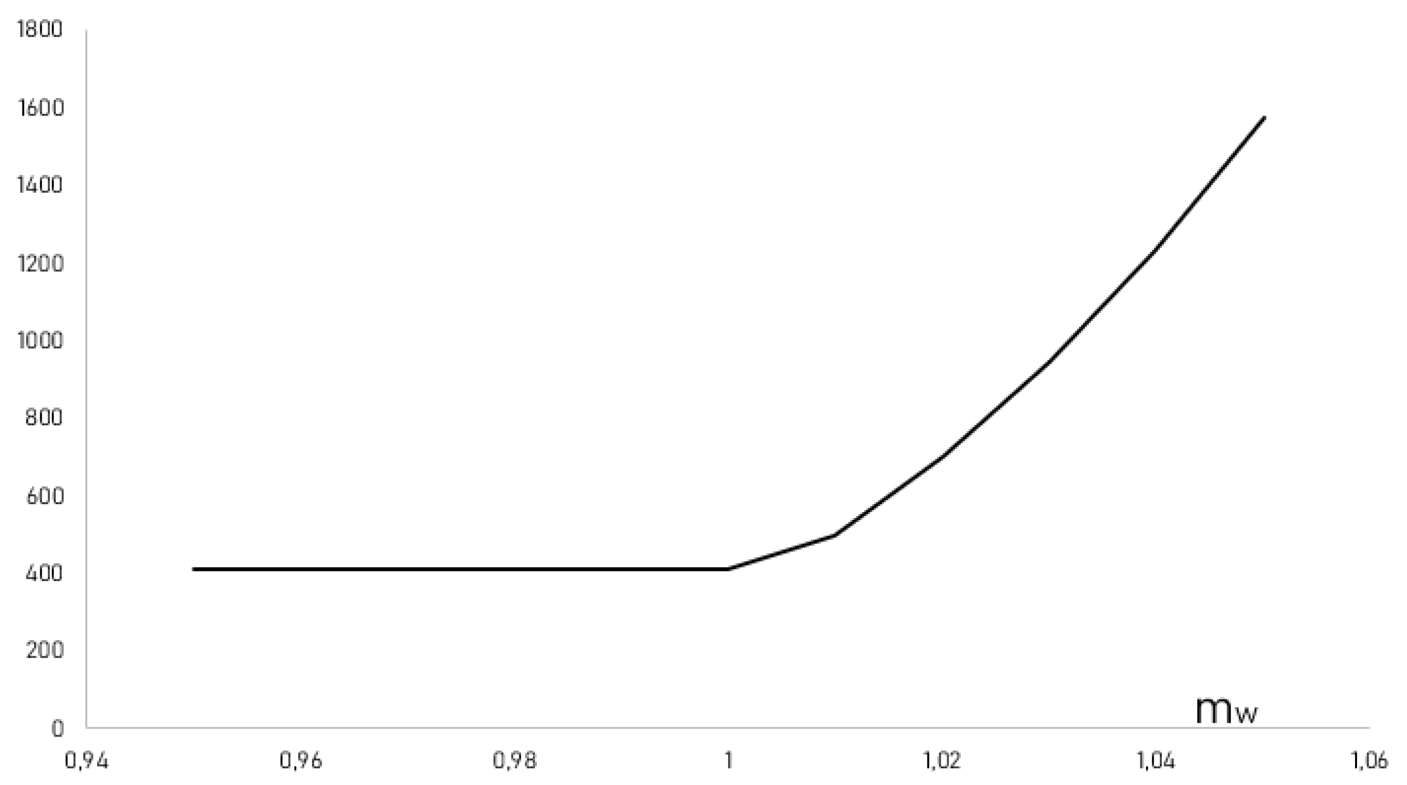
Remark 5. Assuming that there is no medium state, the market is complete and the unique risk-neutral probabilities of the good and bad states are and , respectively. Under that assumption, the discounted expected value of the pension plan isThe present value of all the future contributions under the assumption of completeness is We also picture the effect of the unhedgeable part of the wage to the super-hedging value in
Figure 1. When
is below
,
and hence, the medium state does not affect the value (in both positive and negative relation cases). However, high values of
heavily increase the distance to full hedging, an outcome that reflects the high risk of the pension fund in this case.
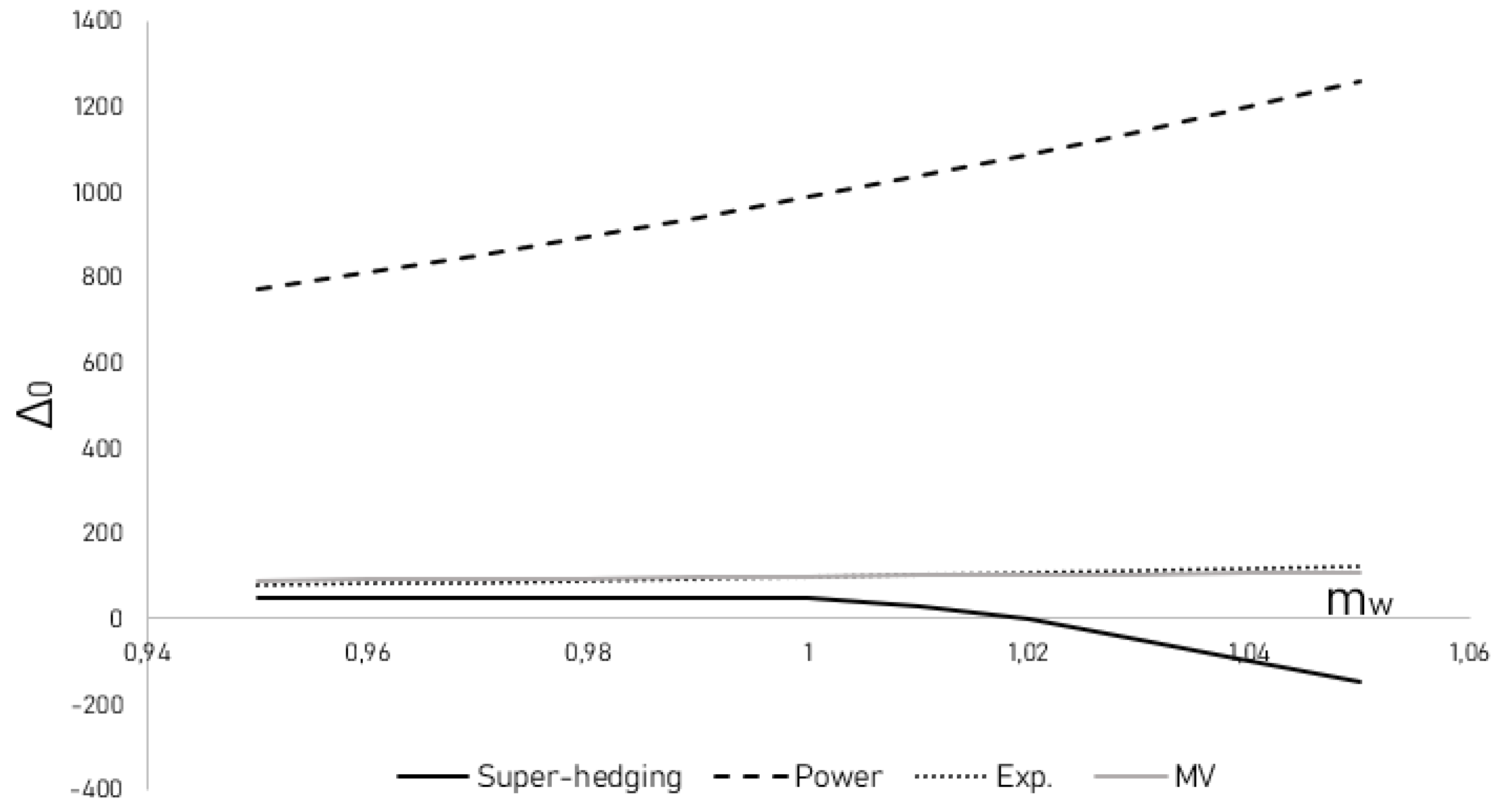
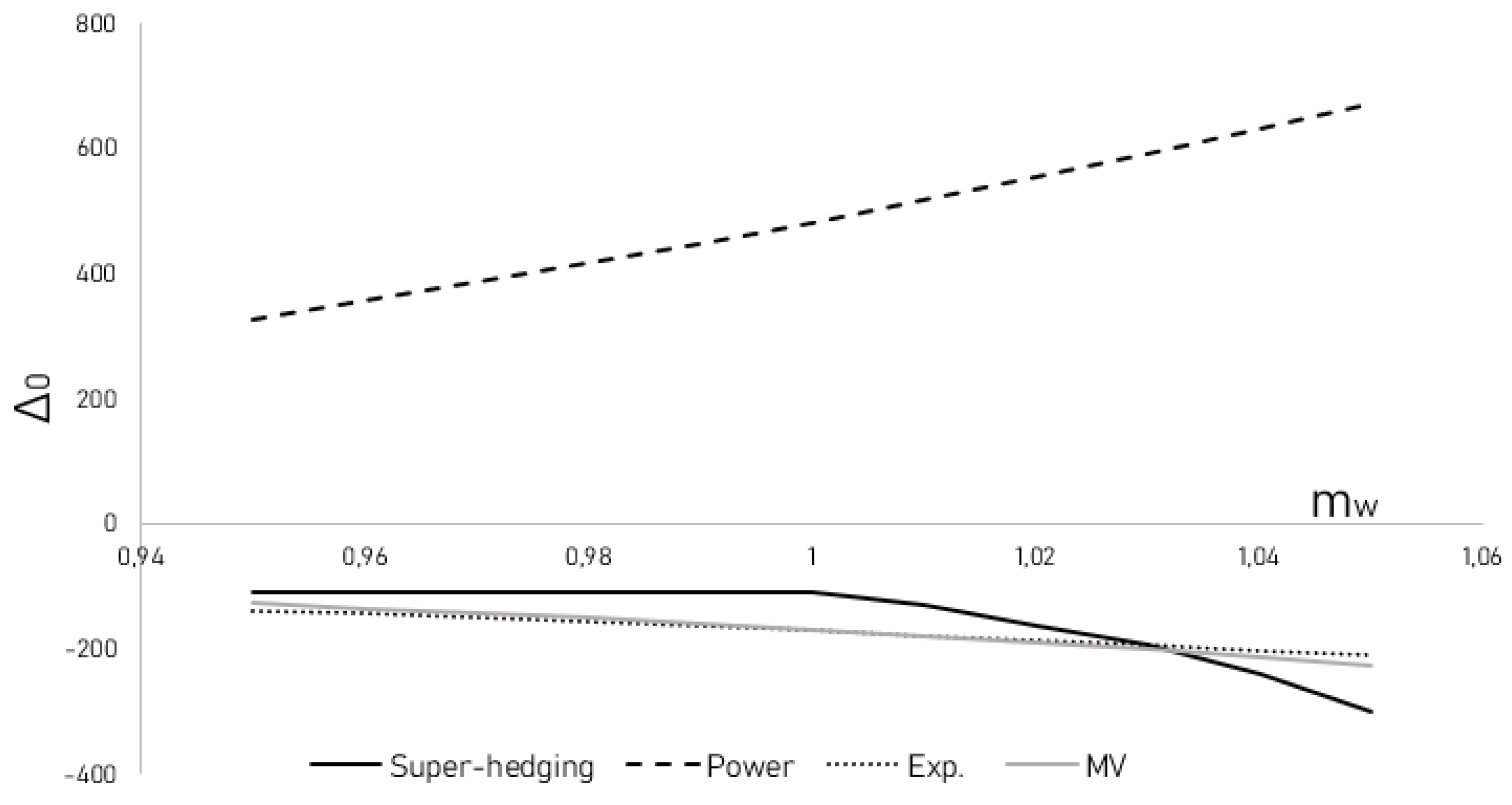
We now consider the utility-based optimization strategies under the condition where
. For this, we demonstrate in
Figure 2 and
Figure 3 the relation between the initial position in the risky assets for super-hedging and utility-based strategies and the unhedgeable part of the wage process. Firstly, we notice that (as stated in Proposition 1) in Case 1,
implies negative
(super-hedging indicates a short position). On the other hand, all the considered subjective strategies suggest positive positions to the risky asset.
12 This example indicates that the subjectivity of a utility maximizer prevails over the objectivity of the hedging goal, even in the case where the goal can be fully hedged, and that the utility maximization is considered on the terminal capital surplus. In other words, due to the positive expected excess return of the risky asset (we used probabilities
,
and
), the optimal strategies are willing to undertake unneeded investment risk and in fact in the opposite direction to the hedging strategy. The situation is more intense under CRRA preferences.
4. The Effect of Early Exit
In the previous sections, we have not considered the possibility of a member’s early exit from the pension plan. This may occur not only if a member dies before the retirement time, but also in the case where the member stops working (at least at the job that is linked to the pension plan). We now incorporate this possibility in our model and under specific assumptions, we update our super-hedging pricing calculations. We consider the case where the exit is random, in the sense that there is an exogenously given sequence of probabilities that a member leaves the pension plan before N. Our main task is to determine the exact conditions in which the possibility of early exit increases the distance to full hedging (i.e., the super-hedging valuation).
In the sequel, for each , stands for the probability that the member remains in the pension plan at period . Hence, so far we have imposed that for all t. It is quite reasonable to assume that these probabilities are non-increasing through time (i.e., the annual probability of exit is not decreasing as the member gets older). While this monotonicity is not necessary to our analysis, the following assumption is both reasonable and very useful.
Assumption 2. The probability of early exit is independent of the risky asset’s price.
Assumption 2 requires that our space become larger, in the sense that at each step we have six possible outcomes briefly described below:
where G stands for the good state (increase in risky asset), M for the medium state, B for the bad state, while S means that the member stays and E that the member exits the plan. Incorporating the possibility of early exit in our model, the set of the risk-neutral measures of probabilities (see (
3) and (
5)) changes and, for each
under Assumption 2, contains the probability measures
of the following form:
where
,
,
,
and the elements of
denote the probabilities of events in (
22) in the same order.
13Since our model considers a DB type of liability, the compensation that a member receives at an early exit should be specifically pre-determined. A reasonable way to do so (also consistent with the setting of the whole pension plan) is that when a member leaves at period
they will receive the payment:
In words, the compensation in the case of an early exit is equal to the promised liability up to the period of the exit, where for the last period we consider the last wage associated with the last contribution. It is important to recall that factors
are normally increasing in time, which means that this setting deters an early exit at the first periods (we shall make this statement precise below). Note that we also stress the consistency of the early compensation with the final payment, in the case of no early exit (
1).
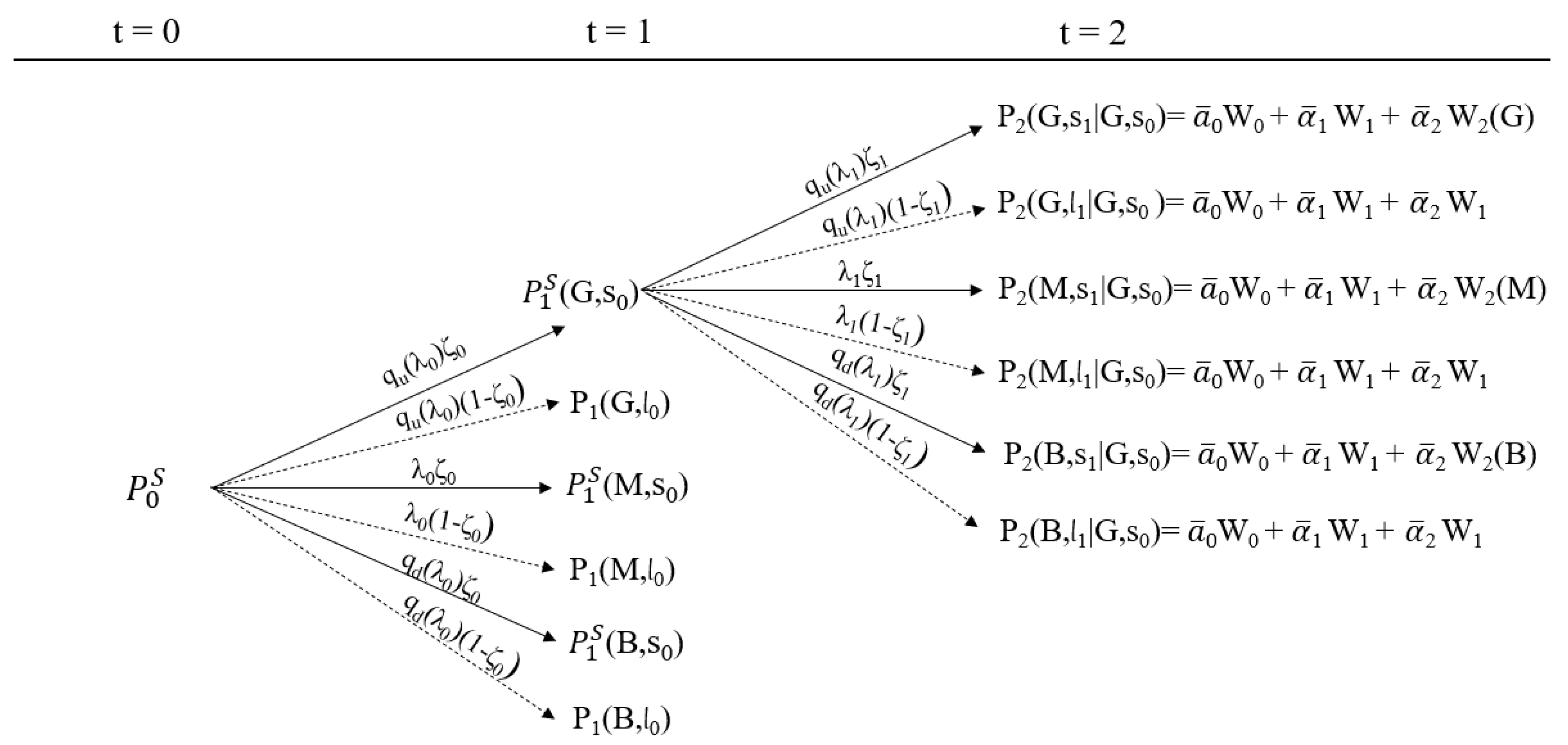
In order to calculate the distance to full hedging for the pension plan under the new setting that allows early exit, we need to construct a tree where at each node there are six possible states. The simplified version of this tree when
is given in
Figure 4.
In order to clarify the way we calculate the super-hedging value in the case of random early exit, we discuss in more detail the case of
. Working backward in time, we assume that we stand at
. At the event of GS in the first period (i.e., the member has stayed in the plan in the period
and the risky asset has increased at this period), the super-hedging value is the maximized expectation of the payoffs shown in
Figure 4. We calculate (and slightly abuse the notation):
where
is the new set of risk-neutral martingale measures,
and
A is given in (
7). Since the above function is linear with respect to
, we obtain the supremum in two possible cases (when
and when
). When
,
becomes consistent with (
9) and, in fact,
whereas when
, we have that
Note that assuming
, the case of
always prevails in the last step of the tree.
Following the same line of argument, we calculate the distance to full hedging at the initial time:
We again have the two possible suprema. When
and when
, we return to the case of no early exit:
Assuming that
, we then obtain that the distance to full hedging increases when random exit is possible if and only if
In the above condition,
denotes the bound of the contribution rate, above which the early exit increases the distance to full hedging of a pension plan. Indeed, when the contribution is sufficiently high, an early exit is harmful for the pension fund (the loss income is higher), given that the liability factors
remain stable. In the same spirit, (
25) indicates that a possible early exit increases the distance to full hedging if the liability factors are sufficiently small (meaning that
is small and hence the condition becomes more likely to hold). Intuitively, smaller liability factors mean that an early exit will cut the (high) contribution inflow in exchange of low liabilities. Finally, note that
is an increasing function of
A, which implies that a low
A has a similar effect to low liabilities. Moreover, a low
A is associated with a narrower wage tree (lower range), which in turn means lower volatility for the liability.
The situation in the general case of
follows the same arguments. In particular, for
, we provide a bound for the corresponding contribution above which the distance to full hedging increases (similarly to (
25)). We state the exact condition in the proposition below.
Proposition 3. Impose Assumption 1 and let . For the pension plan (24) under possible early exit, we have the following: - (i)
The distance to full hedging does not increase when early exit is possible if and only if for each - (ii)
If for each , the distance to full hedging of the pension plan is given by
Remark 6. One of the main useful features of the distance to full hedging as an indicative valuation of a pension plan is the fact that it is not affected by the subjectivity of the probabilities. In particular, in this section, the super-hedging is not affected by the actual level of the probabilities of exit. Rather, the level of the standard inputs of the problem determine whether and how the price is going to change. As we have mentioned in the case of , early exit will not affect the distance to full hedging if the contributions are sufficiently low and the liability factors (and/or parameter A) are sufficiently high. These notices are apparent in condition (26). 5. Conclusions
We have studied the case of a pension fund with defined-benefit liabilities that stem from a linear function of the members’ wage process. The pension fund receives contributions and invests them in a (correlated to the wage) financial market in a discrete-time manner. We consider the liability as the payoff of a path-dependent derivative security. The untradeability of the wage process makes the market incomplete and hence, the pension’s fund liability cannot be fully hedged at a non-arbitrage initial cost. Under that perspective, we propose that the difference between the cost of full hedging and the current pension’s fund capital is a meaningful measure of the distance to fully hedged liability. While in diffusion models the super-hedging value could be problematic from a practical standpoint, in discrete-time and -space market models we are able to obtain closed-form expressions not only for the value, but also for the induced investment strategies.
In that direction, we adapt the simplest possible incomplete model (i.e., a trinomial tree) and analyze the related formulas. From those, we find that the distance to full hedging is basically affected only by the unhedgeable part of the wage process. In fact, a negative relation between the wage and risky asset processes tends to increase the distance to full hedging when the risky asset has high volatility, while when the unhedgeable part of the wage price is too high, the risky asset volatility could be hedged out and hence, it does not affect the valuation. As for the super-hedging investment strategy, we find that a positive (resp., negative) relation between the wage and risky asset results in a positive (resp., negative) position in the risky asset (provided that the unhedgeable part of the wage is not extreme). Furthermore, a higher liability (resp., contributions) implies a higher (resp., lower) investment (in absolute value) in the risky asset.
Furthermore, we use a utility-based optimization portfolio to point out that in cases of sufficient capital, the application of a subjective investment criterion may result in heavily different strategies than the super-hedging one. In these situations, the pension fund will be left with some liability risk, although it could have been fully hedged. Finally, we provide conditions under which the effect of a possible random early exit leaves the distance to full hedging unchanged. In particular, this holds when the contribution factor is sufficiently low and/or the liability factors are sufficiently high.
The super-hedging value is a meaningful way to measure the positive effects of a dedicated-to-hedging liability-driven strategy. Having established the well-posedness of the notion of super-hedging valuation in discrete-time and -space models, several possible extensions emerge. For example, one could consider larger incomplete-market trees that could allow the use of more risky assets and then examine how the super-hedging value changes when the investment pool is extended. Another extension could deal with the function that determines the liability payment. Herein, we have considered a linear function that in principle could be generalized in more flexible, hybrid payment structures. Another possible extension is to examine how the option of an early exit by a member (which is possible in pension funds with voluntary participation) could affect the super-hedging value and strategy. From the proposed setting, a number of unquestionably interesting questions that can be subjects for future research.


