Article

Whoops! It Happened Again: Demand for Insurance That Covers Multiple Risks †

1
Department of Mathematical Sciences, The University of Texas at Dallas, Richardson, TX 75080, USA
2
Department of Economics, Finance, and Legal Studies, University of Alabama, Tuscaloosa, AL 35487, USA
3
Alabama Center for Insurance Information and Research, Culverhouse College of Business, University of Alabama, 1500 Greensboro Ave Suite 2, Box 870397, Tuscaloosa, AL 35487, USA
*
Author to whom correspondence should be addressed.
This article was completed after the untimely passing of Dr. Harris Schlesinger. His contribution to this article is significant. However, any remaining errors are entirely our own and in no way attributed to him. This article is dedicated to his memory.
Risks 2023, 11(4), 73; https://doi.org/10.3390/risks11040073
Submission received: 23 February 2023 / Revised: 29 March 2023 / Accepted: 6 April 2023 / Published: 10 April 2023
(This article belongs to the Special Issue Frontiers in Quantitative Finance and Risk Management)

Abstract

:
This article studies insurance demand in a two-period framework in which an individual faces risks in both current and future periods. Models for insurance with and without the presence of endogenous saving are both discussed. In contrast to what most literature suggests, when decisions on insurance and saving are made separately, insurance alone does not always unambiguously reduce risk, and decision makers might demand more insurance when there is a positive loading on the premium than when the insurance price is actuarially fair. We compare the demand for insurance in our framework with that in a two-period model where risk is concentrated in the second period and derive the conditions under which these demands differ. We examine the effects of risk aversion and derive the conditions under which a more risk-averse individual demands more or less insurance.

1. Introduction

How does insurance work? Take automobile insurance for example: Once a contract is agreed upon and a premium is paid, the insurance provides financial protection against physical damage, bodily injury, and potential liability resulting from vehicle collision. The contract often lasts for six months, during which time, multiple incidents are possible. Meanwhile, when making decisions for insurance, people might or might not make joint decisions for transferring wealth across periods (Hofmann and Peter (2016)). Therefore, to study the decision-making process for purchasing insurance, one should take into account these characteristics of an insurance contract. However, to the best of our knowledge, no studies have been undertaken to incorporate these aspects into a single model.
First of all, to study the effects of the separate timing of paying a premium and incurring a loss, an intertemporal model is needed. Most insurance articles (Mossin (1968); Schlesinger (1981); Briys (1986); Somerville (2004); Schlesinger (2006)) use either a one-period model or a continuous-time model in which insurance decisions and potential loss happen simultaneously. Some works, especially more recent ones, intertemporally separate costs and benefits (Dionne and Eeckhoudt (1984); Menegatti (2009); Hofmann and Peter (2015); Peter (2017)). These works lay the foundation for exploring the demand for insurance in a two-period framework.
Secondly, the model needs to address the possibility of multiple losses during the insurance contract period. Risk reduction in the presence of multiple risks has drawn attention from many researchers. However, previous literature has focused mostly on multi-dimensional risks instead of multi-period ones. Raviv (1979) presents a single-period model which incorporates the case of two potential losses. Doherty and Schlesinger (1983) examine insurance decisions when there is a second uninsurable correlated risk. Gollier and Scarmure (1994) analyze the issue for the case of uncorrelated risks. Fluet and Pannequin (1997) extend the standard adverse-selection model for insurance to the case where individuals are subject to multiple risks. Bonato and Zweifel (2002) conduct an empirical analysis of insurers’ information about multiple risks. Courbage et al. (2017) analyze optimal prevention expenditures in a situation of multiple correlated risks. Seog and Hong (2022) analyze insurance demand and saving in a two-period model with multiple loss states. We examine in this paper an insurance contract covering two periods with the possibility of a loss at each period.
In addition to allowing multiple occurrences of losses, our model also considers how the timing of the loss will affect the decision maker’s choice on insurance purchase. Consider the case when an individual purchases an insurance covering (part of) the potential losses for one year. Whether a loss occurs soon after the purchase or near the end of the year obviously makes a difference. If a loss occurs right after the purchase, the individual experiences the effect of reduction in consumption resulting from both the cost of insurance and the loss itself (in the case of partial coverage). On the other hand, if a loss occurs towards the end of the year, it only affects the consumption level during that period.
Last but not least, the potential interaction between insurance and saving plays a vital role in the decision-making process. While it is normally assumed that wealth is perfectly fungible, Thaler (1999) shows that mental accounting violates this economic assumption, which suggests that money spent on insurance might not be a perfect substitute for money invested in saving. Hence, from the individual’s perspective, the insurance decision and the saving decision could be separable. With this in mind, we present two settings for insurance demand, one with and the other without endogenous saving.
In this paper, we look at paying a premium at a date t = 1 and then incurring potential losses (and potential indemnities) at both dates t = 1 and t = 2 . We investigate the case where insurance and saving decisions are undertaken separately as well as the case where they are undertaken jointly. Our paper contributes to the literature by developing a theoretical model which not only describes the time structure of paying insurance premiums upfront, but also allows the possibility of multiple losses. The results help to explain some empirically observed deviations of insurance demand from those made with previous one- or two-period models. The paper is organized as follows: Section 2 presents a model of insurance, followed by extending the model to incorporate endogenous saving (which also includes borrowing). The optimal levels of insurance in both settings are analyzed and compared with those obtained from models in which risk is concentrated in the second period. The effects on riskiness in both models are investigated. Section 3 examines the effects of risk preferences. Section 4 concludes the paper.

2. The Models and the Results

This section presents the models and compares the results with those obtained from models in which a loss state is only possible during the second period. We present two different settings, one for the case where the insurance decision and the saving decision are separable, the other for the case where the individual integrates the decision for saving when purchasing insurance.

2.1. Optimal Insurance

First, we analyze the optimal level of insurance in the absence of endogenous saving. The model presented in this section corresponds to situations where an individual either forgoes her choice of saving or saves/borrows but does not integrate this into her decision-making process of insuring the risk.
Assume that a representative individual is endowed with W in both the current and the future periods and also faces the risk of losing l in both periods. The distributions of such losses in these two periods are independent to each other. The possibilities of loss during the current and the future periods are, respectively, π [ 0 , 1 ] and δ [ 0 , 1 ] . As we assume only two states of the world are possible, 1 π and 1 δ are the possibilities that no loss occurs in the respective periods. For simplicity, we assume both the subjective time discount rate and the rate of gross risk-free return are equal to one.
In this environment, the individual chooses at the current period the insurance coverage, α [ 0 , 1 ] , to maximize expected utility over the two periods:
E ( U ) π u ( W α P l + α l ) + ( 1 π ) u ( W α P ) + δ u ( W l + α l ) + ( 1 δ ) u ( W ) ,
where P = ( 1 + λ ) [ π l + δ l ] denotes the insurance premium, and λ , the proportional loading ( λ = 0 in the case of a marginally fair premium).
To examine the effects of incorporating risks in both periods, we compare the optimal demand for insurance with that of a two-period model in which a loss state is only possible during the second period. This benchmark model is given as:
E ( U b ) u ( W α P ) + q u ( W L + α L ) + ( 1 q ) u ( W ) ,
where q = π + δ 2 is the probability of losses during the second period, and L = 2 l is the size of such loss. These specifications ensure that the expected losses, as well as the maximum possible losses over the two periods are the same between the two models. We acknowledge that it is a bit odd to assume L = 2 l , but notice that 0 < π + δ < 2 , so if we keep loss severity fixed and only vary the probabilities (i.e., L = l and q = π + δ ), we not only eliminate half of the possibilities by constraining them as π + δ < 1 , but also have a different maximum possible loss.
The following numerical example may help to illustrate the impact of different timings of risks. 
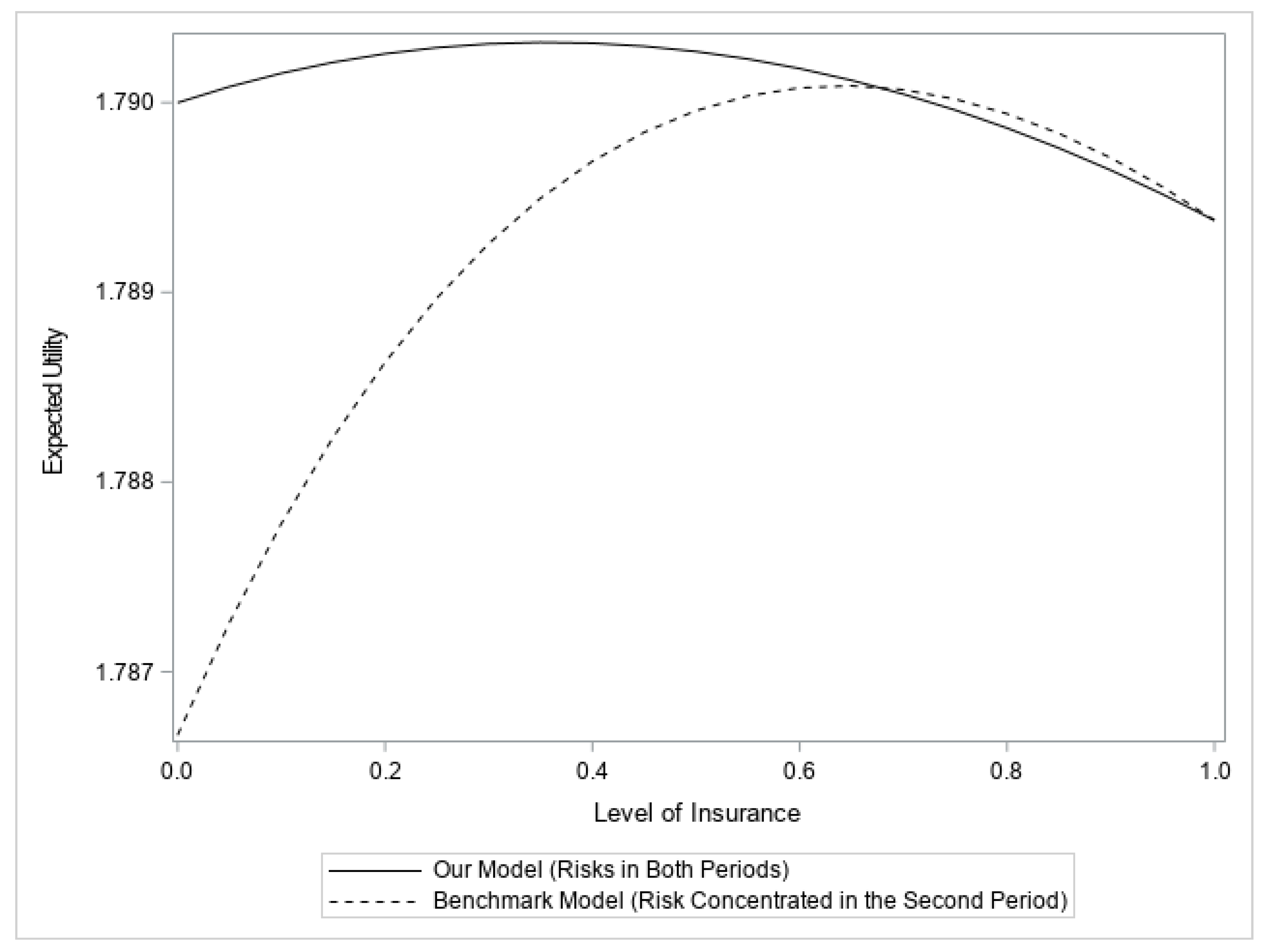
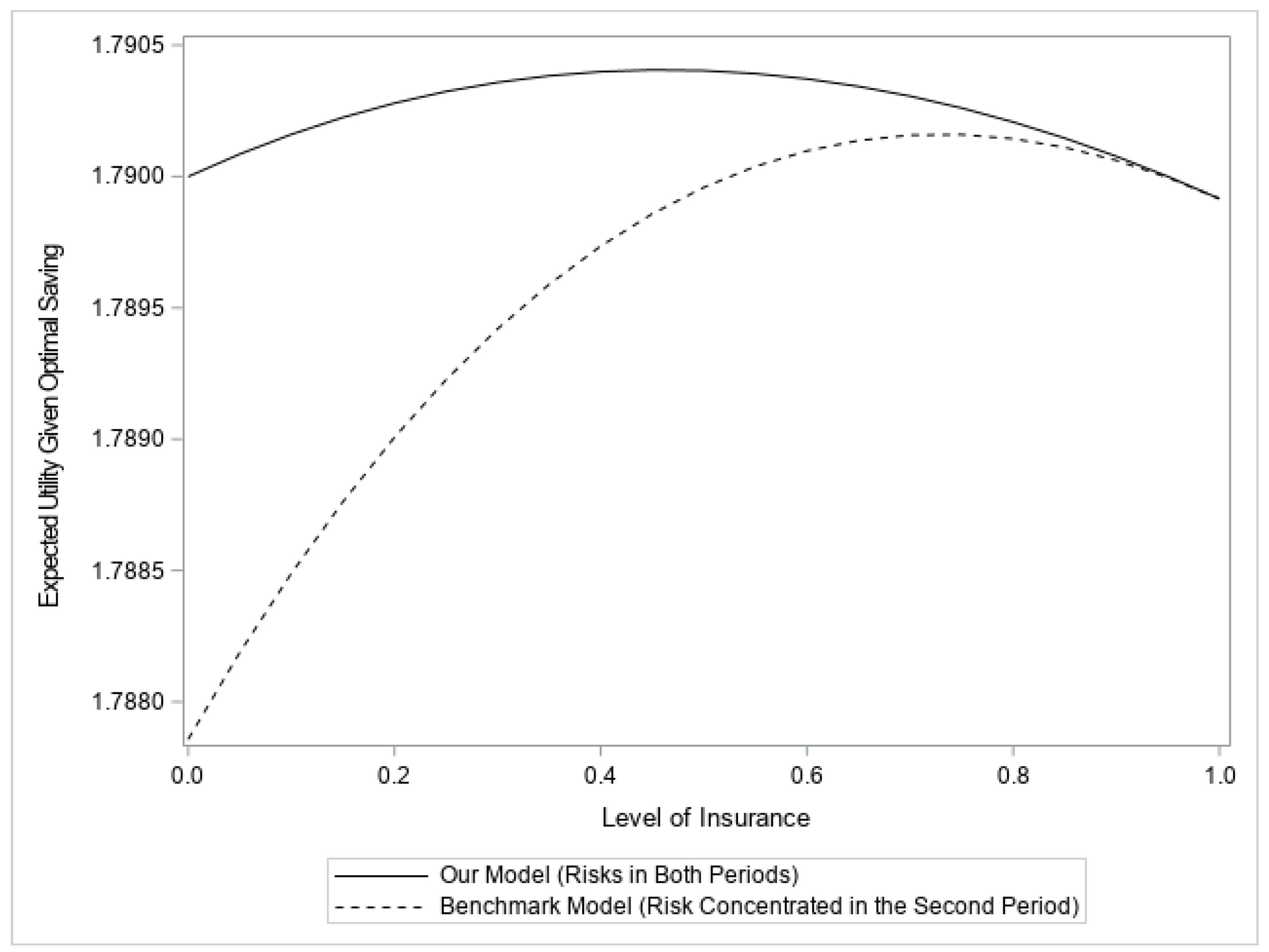
Figure 1 provides a direct impression of the differences between the two models. Though both the maximum possible loss and the expected loss of our model are the same as those of the benchmark model, our model not only has a higher maximum expected utility, its optimal level of insurance is also different from that of the benchmark model.
Next, we will formally compare the optimal insurance of our model and that of the benchmark model. It is straightforward to show that the second-order conditions are satisfied for both models as long as the individual is risk-averse ( u < 0 ). Hence, the optimal levels of insurance in each setting can be characterized by the respective first-order conditions. With this in mind, we derive the following propositions:
For a zero loading, λ = 0 , we have:
Proposition 1.
a. A risk-averse individual demands less than full insurance.
b. When π + δ 1 , the decision maker demands less insurance coverage than when risk is concentrated in the second period.
c. Otherwise, the decision maker purchases less/equal/more insurance when π + δ > / = / < Ω 1 , where Ω 1 is an endogenously determined threshold.
Proof. 
See Appendix A.1. □
It is noteworthy that the level of consumption at the no-loss state in the second period is not permutable. Insurance decreases the consumption gaps between the respective loss and the no-loss states in both the current and the future periods. However, the cost of purchasing insurance in the first period increases the consumption gap between the no-loss state in the first period and the no-loss state in the second period, as well as the gap between the loss state in the first period and the no-loss state in the second period. Therefore, insurance is an imperfect way of smoothing consumption over time in this model. The individual purchases less than full insurance even when the insurance premium is actuarially fair, which implies Mossin’s Theorem is violated. Given the optimal level of insurance for the benchmark model, when the sum of the probabilities of losses for the two periods is larger than one in our model, the marginal cost of purchasing insurance is always greater than the expected marginal benefit, suggesting a decrease in the demand of insurance. Otherwise, the decision maker purchases less insurance than when risk is concentrated in the second period if the sum of the probabilities of losses is larger than a threshold and vice versa.
Let us now consider the case when there is a positive premium loading, i.e., λ > 0 . Let α ˜ * denote the optimal insurance coverage when risk is concentrated in the second period, we have:
Proposition 2.
a. Compared to the optimal level of insurance when the price is actuarially fair, when π + δ 1 1 + λ , a decision maker always demands less insurance; when π + δ < 1 1 + λ , a non-decreasing absolute prudence is the sufficient but not necessary condition for an individual to demand less insurance;
b. When π + δ 1 α ˜ * α ˜ * ( 1 + λ ) or π + δ 1 1 + λ , the optimal demand for insurance is lower than that when risk is concentrated in the second period;
c. Otherwise, the optimal demand for insurance is lower/equal/higher when ( 1 + λ ) ( π + δ ) > / = / < Ω 2 , where Ω 2 is an endogenously determined threshold.
Proof. 
See Appendix A.2. □
Unlike Mossin’s Theorem, the individual does not purchase full insurance with an actuarially fair premium. More importantly, the decision maker might purchase more insurance when the premium becomes unfair. Given the optimal level of insurance when the price is actuarially fair, a positive loading on the insurance premium increases the marginal cost of purchasing insurance, as well as the marginal benefits of insuring in both periods. If the probabilities of losses are large enough, the increases in the marginal cost always outweigh the increases in marginal benefit for the loss state in the first period, resulting in a lower demand for insurance. On the other hand, if the probabilities are small, a non-decreasing absolute prudence1 ensures the increases in marginal cost are more than the increases in marginal benefits for the loss states in both periods. This is important because standard risk aversion requires decreasing absolute prudence (Kimball (1993)), implying that it is possible for an average decision maker to purchase more insurance when the price becomes unfair.
When individuals make insurance decisions, they face several uncertainties. First, they do not know whether the losses will occur or not over the two periods. Second, they do not know how many losses will occur. Lastly, when a loss occurs, they are uncertain whether it will happen during the first period or the second one. Therefore, the individuals need to take into account all the uncertainties during the decision-making process.
Propositions 1 and 2 summarize such effects. Besides the deviation from Mossin’s Theorem, it is also interesting to observe that when the cost of insurance is within a certain range, whether the decision maker demands more or less insurance than when risk is concentrated in the second period depends on whether the price is lower or higher than a threshold. Notice that a higher cost of insurance does not necessarily mean a larger premium loading; it can also mean the risk is greater, in the sense that the sum of the probabilities of losses for the two periods is larger.
For an illustration, we compare the degree of riskiness in our model with that of the benchmark model where risk is concentrated in the second period. In a two-period model with a zero time discounting rate, one can multiply all the probabilities by 1 / 2 . Then, without loss of generality, the wealth prospects are the same ones as in the setting of a single-period model. Therefore, we can use an illustration similar to the one in Briys and Schlesinger (1990). First, we compare the risks in the two models. Even though we construct our model so that the expected loss, as well as the probable maximum loss, are the same as those of a benchmark model, the risks, as defined in Rothschild and Stiglitz (
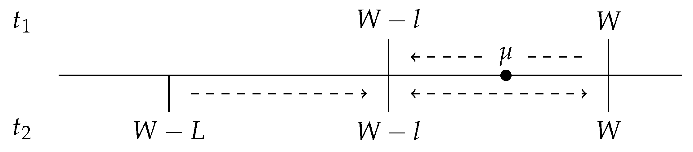
1970), are different. Under the assumption of a zero time discounting rate, we can normalize the sum of the probabilities for the four states to one. Then, an individual’s wealth prospects over the two periods for both models can be illustrated as shown in Figure 2.
For the benchmark model, the individual’s wealth is W plus a lottery between W L and W. For our model, the individual’s wealth is the sum of two lotteries between W l and W. By construction, these two models have the same expected wealth, μ , over the two periods. Essentially, from the benchmark model to our model, some of the probability mass ( 1 2 π ) is shifted from W to W l during the first period, while in the second period the entire probability mass ( 1 2 q ) is shifted from W L to W l and/or W. Moreover, some of the probability mass might shift from W to W l , resulting in a probability mass of 1 2 δ at W l and a probability mass of 1 2 ( 1 δ ) at W. Ultimately, the two probability masses in the benchmark model, W and W L , are shifted to W and W l in our model. Such a shift is a mean-preserving contraction of the wealth distribution, representing a decrease in risk. Therefore, the situation faced by the decision maker in our model is less risky than the one faced in the benchmark model.
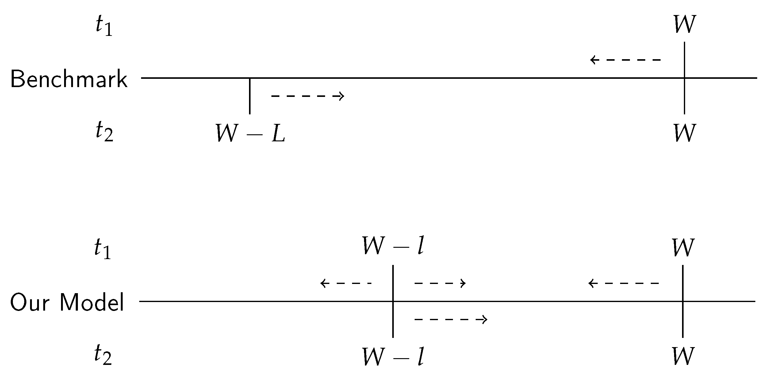
Now, consider the case of insurance. Again, we normalize the sums of probabilities to one, and the individual’s wealth prospects can be illustrated as in Figure 3. Assuming the same level of insurance for both models, in the benchmark model, final wealth in the first period is reduced by α P , while final wealth in the loss state in the second period is increased by α L . In our model, final wealth in the no-loss state in the first period is reduced by α P , while final wealth in the loss state in the second period is increased by α l . As for the loss state in the first period, whether final wealth increases or decreases depends on the sign of P + l . Because the expected loss is the same for both models, the expected wealth over the two periods is also the same given the same loading factor λ .
In our model, when P + l 0 , W α P l + α l W l . It suggests that the effect of insurance causes both a (mean-preserving) spread and a (mean-preserving) contraction in the wealth distribution, so that it is less effective compared to its effects in the benchmark model, in which it always represents a (mean-preserving) contraction. Mean-preserving is achieved when the insurance price is actuarially fair. We have already illustrated that there is less risk in our model. Therefore, as shown in Propositions 1 and 2, when π + δ 1 with λ = 0 or when π + δ 1 1 + λ with λ > 0 , the decision maker always demands less insurance coverage than when risk is concentrated in the second period.
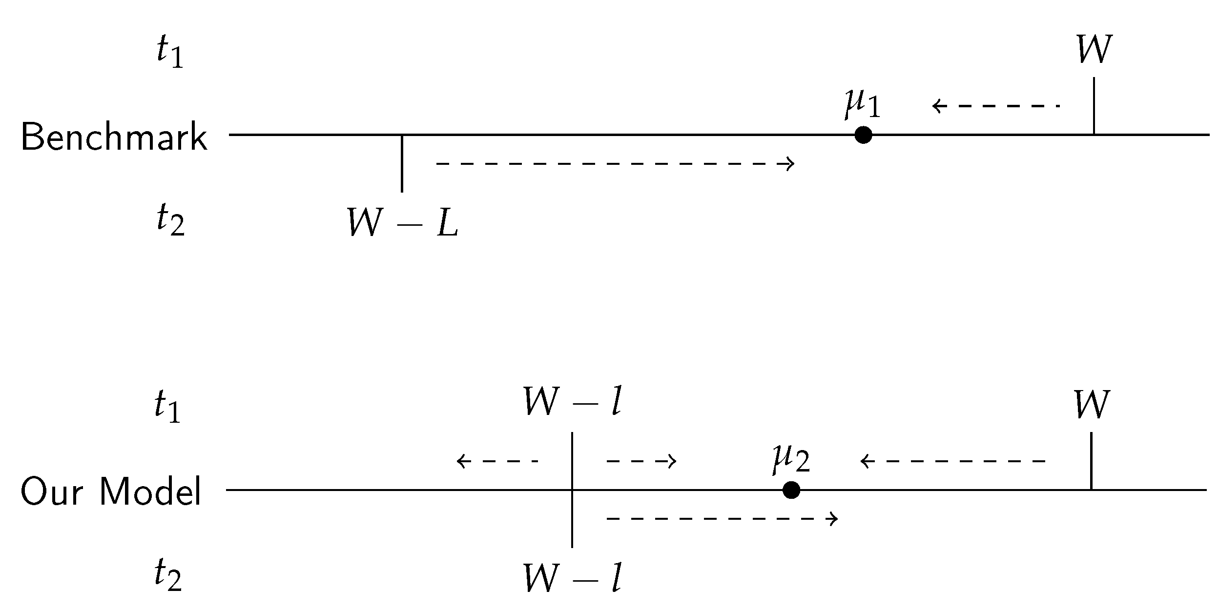
On the other hand, if we focus on the states that are affected by the choice of insurance and normalize the sums of these probabilities to one, we can illustrate the individual’s wealth prospects as in Figure 4.
μ 1 = E ( w | 1 , 2 L ) and μ 2 = E ( w | 1 , 2 l ) are the expected levels of wealth given a loss state occurs in the second period for the benchmark model and our model, respectively. Consider the case when λ = 0 . We have μ 1 = W q 1 + q L and μ 2 = W π + δ 1 + δ l = W q 1 + δ L . Thus, the optimal level of insurance for the benchmark model is α ¯ * = 1 1 + q , and the two probability masses of W and W L are shifted to μ 1 . In our model, insurance cannot equate the levels of wealth for all three states to μ 2 .
We have shown that when π + δ 1 the decision maker always demands less insurance compared to that in the benchmark model. If π + δ < 1 , things are not quite straightforward. Applying α = α ¯ * to the model, we have w 1 l = W 3 2 q L 1 + q < μ 2 , w 2 l = W 1 2 q L 1 + q > μ 2 , and w 1 n l = μ 1 , where w 1 n l , w 1 l , and w 2 l are the levels of wealth for the three states. Increasing the level of insurance will move the probability mass of w 1 l closer to μ 2 while moving w 2 l further from it. We know an increase in insurance will move the probability mass of w 1 n l to the left, but because μ 1 < / = / > μ 2 when π < / = / > δ , whether the probability mass will move closer or further from μ 2 remains endogenously determined. Therefore, even though the insured risk is less risky in our model and the insurance itself might not be as effective, the decision maker could still demand more insurance.

2.2. Optimal Insurance and Optimal Saving

In the previous model, we exclude the possibility of saving in order to focus our inquiry on the case when the decisions for saving do not play a role in the determination of optimal insurance. Here, we examine the situation when the decisions for insurance and saving are made jointly.
In addition to consuming and purchasing insurance, individuals also decide how much they want to save or borrow at Period 1. We denote by S the individual’s savings. Note that S stands for saving for S > 0 , and borrowing for S < 0 . The individual’s objective function then changes to:
U π u ( W α P l + α l S ) + ( 1 π ) u ( W α P S ) + δ u ( W l + α l + S ) + ( 1 δ ) u ( W + S ) .
When endogenous saving can be used to achieve consumption smoothing, the second-period wealth in the no-loss state is affected by the individual’s decisions. Mossin’s Theorem can be proved with this model:
Lemma 1.
With endogenous saving, an individual purchases full insurance if and only if the premium is actuarially fair.
Proof. 
See Appendix A.3. □
This is reminiscent of the Separation Theorem obtained by Dionne and Eeckhoudt (1984), in which endogenous saving is described implicitly. In addition, our finding extends Mossin’s Theorem to a two-period setting in which both periods are subject to the risk of loss. With a zero premium loading, full insurance ( α = 1 ) equates the consumption level of the loss state and that of the respective no-loss state in each period. The corresponding saving choice, S = ( π + δ ) l 2 , equates the levels of consumption in t = 1 and t = 2 .
On the other hand, even though the levels of consumption across periods/states can still be equalized, a positive premium loading causes insurance (or sacrificing saving/increasing borrowing to fund insurance purchase) to generate a cost of lower aggregate consumption over time. Therefore, it is not optimal to purchase full coverage. In conclusion, Mossin’s Theorem is restored for the model with both insurance and endogenous saving.
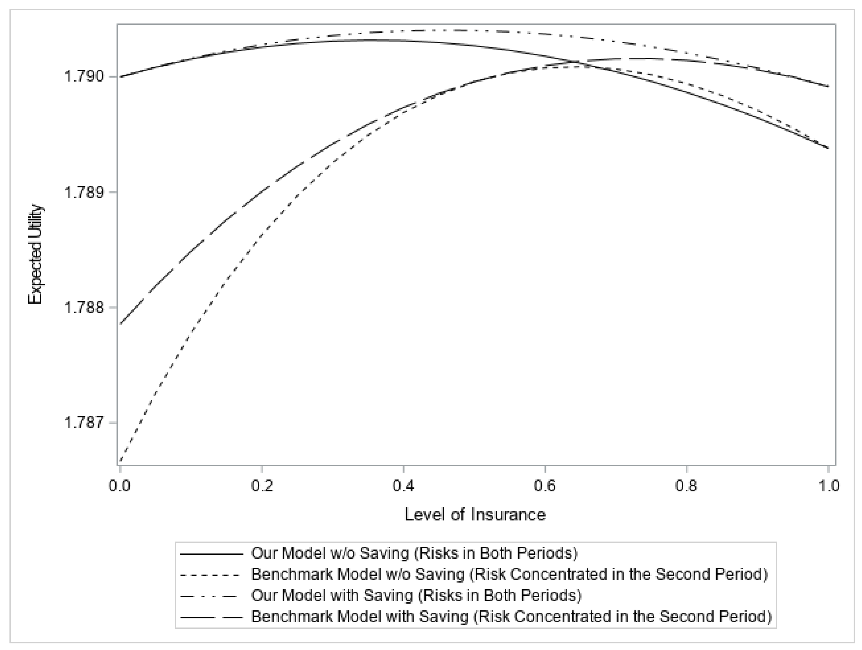
Figure 5 illustrates the differences between our model and the benchmark model with the presence of endogenous saving. The expected utilities are calculated with the optimal levels of saving given different levels of insurance. Even when the decision maker can shift wealth between periods, the different timings of losses still have a profound effect on the optimal demand for insurance. When compared with Figure 12, we notice that the presence of endogenous saving increases both the maximum expected utilities and the optimal levels of insurance for both models, but the difference between the two optimal insurance levels still persists.
As discussed in Hofmann and Peter (2016), because both insurance and saving are endogenous, the saving choice that is optimal for one level of insurance is typically not optimal for other levels of insurance. Thus, we cannot directly plug the first-order condition of one model into that of the other model and check the sign. Therefore, comparing the optimal choice of insurance with that of the benchmark model in which risk is concentrated in the second period seems difficult. Fortunately, using the method proposed by Gollier (2004), we are still able to investigate the effects of having risks in both periods. The results are summarized in the following proposition:
Proposition 3.
When ( 1 + λ ) ( δ + π ) > / = / < Ω 3 , the optimal demand for insurance is lower/equal/higher than that when risk is concentrated in the second period, where Ω 3 is an endogenously determined threshold.
Proof. 
See Appendix A.5. □
Endogenous saving helps individuals achieve better consumption smoothing and changes the optimal level of insurance. Individuals purchase full insurance with an actuarially fair price. When there is a positive premium loading, comparing the optimal demand for insurance with that of the benchmark model in which risk is concentrated in the second period shows that the decision maker demands less insurance when the cost of insurance is higher than a threshold and vice versa. Again, a higher cost of insurance can be the result of either a larger premium loading or a larger sum of the probabilities of losses for the two periods or both.
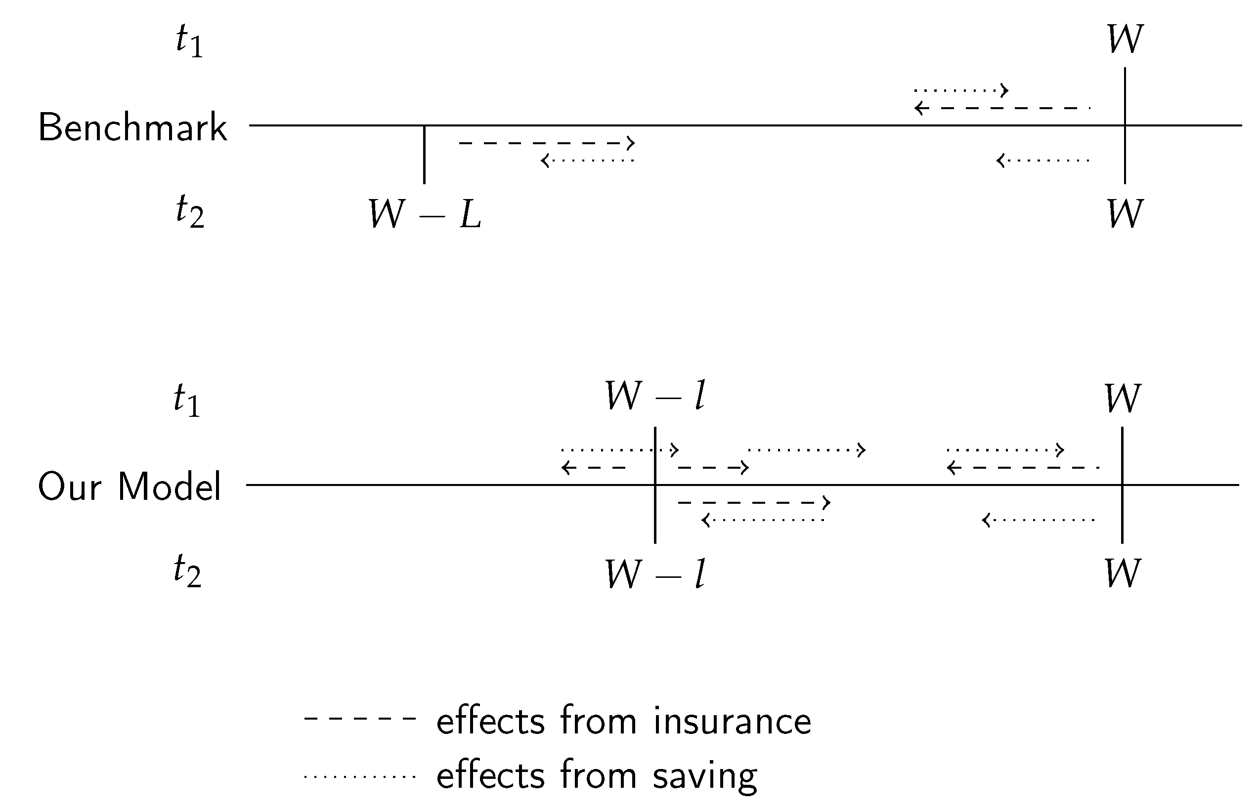
As for the effects on riskiness, when taking into account endogenous saving, the decision maker can move wealth between periods. If the endowments are the same in both periods, we have shown that the individual will borrow in the first period. The individual’s wealth prospects are illustrated in Figure 6.
As can be seen from Figure 6, in each model, borrowing moves some of the wealth from the second period to the first one. Thus, even though insurance might still cause a spread in the wealth distribution, this effect can be “fixed” by borrowing from the future. Therefore, whether the decision maker purchases more or less insurance than one would if risk is concentrated in the second period is now determined endogenously, as we shown in Proposition 3.

3. Effects of Risk Aversion

3.1. Model with Independent Insurance Decision

Assume individual V’s utility function is more concave than that of individual U. Her utility function can be described as v, where v is a concave transformation of u. Following Pratt (1964), v = k ( u ) , with k > 0 , k < 0 . As mentioned in Hofmann and Peter (2016), the concavity of the individual’s utility function in a two-period model measures the resistance to consumption fluctuations across both different states and periods.
Proposition 4.
Let individual V be more risk averse than individual U. The sufficient (but not necessary) condition for V to purchase more insurance than U is that U’s consumption in the loss state of the first period is not less than in the loss state of the second period.
Proof. 
See Appendix A.6. □
This finding is similar to the result in Hofmann and Peter (2016), where they suggest the individual with a more concave utility invests more in self-insurance if and only if individual U’s Period 1 consumption exceeds her Period 2 consumption in the loss state. However, unlike Hofmann and Peter (2016), where the condition is necessary and sufficient, the condition in our finding is sufficient but not necessary. This is similar to the finding in Seog and Hong (2022)’s two-period model with multiple loss states in the second period. Our model, allowing the loss to happen in both periods, provides a condition that is based on the relationship between the consumption levels of the two loss states. If individual U’s level of consumption in the loss state of the first period is not less than in the loss state of the second period, purchasing more insurance will close the gap between these two levels of consumption. On the other hand, if individual U’s level of consumption in the loss state of the first period is less than in the loss state of the second period, reducing the amount of insurance purchased will close the gap between these two levels of consumption. Because individual V has a larger desire to smooth consumption, these reductions in the consumption volatility are beneficial to her.

3.2. Model with Endogenous Saving

Again, consider individual V whose utility function is specified as v = k ( u ) , with k > 0 and k < 0 .
Proposition 5.
When endogenous saving presents, an individual with a more concave utility
a. Purchases more insurance when ( 1 + λ ) ( π + δ ) < π 1 δ ;
b. Never purchases more insurance when the price is actuarially fair;
c. Purchases less insurance when ( 1 + λ ) ( π + δ ) > max ( 1 , π 1 δ ) .
Proof. 
See Appendix A.7. □
Note that both conditions are sufficient but not necessary. The above proposition shows that with endogenous saving, a decision maker with a more concave utility does not always demand more insurance. In fact, she might even purchase less insurance. This finding is different from the results in Hofmann and Peter (2016) and Seog and Hong (2022), where they show an agent with more concave utility always selects more self-insurance. When the cost of insurance is high and the probability of loss during the second period is relatively low compared to that during the first period, the “risk” of no loss occurring during the second period causes the individual to reduce her insurance demand. Even though endogenous saving helps the individual achieve consumption smoothing across periods, unlike the case where risk is concentrated in the second period and the choice of insurance is entirely devoted to mitigating the risk, here the choice of insurance still plays a part in improving the individual’s consumption stream. Recall that the concavity of the utility function in a two-period model measures the resistance to consumption fluctuations across both different states and periods. Hence, an increase in the concavity might cause the expected cost of purchasing insurance and having a loss during the first period outweigh the expected benefit of having insurance during the second period, thereby causing the individual to purchase less insurance.

4. Conclusions

The two-period model we present in this paper better describes the time structure of paying an insurance premium upfront and allows the possibility of having multiple losses over the two periods. The model also distinguishes the timing of the losses. In addition, endogenous saving enriches people’s options, enables them to smooth their levels of consumption across periods/states, and achieve a better total outcome.
There are several interesting findings generated from this structure. First of all, we show that Mossin’s Theorem is violated when saving is absent. People purchase less than full insurance even with an actuarially fair price. More importantly, people might increase their insurance purchases when the price becomes unfair. Once we introduce endogenous saving into the model, people have the ability to smooth their levels of consumption across periods and states and are able to achieve the first-best outcome. Mossin’s Theorem is restored for this setting. Insurance and saving jointly allow enough degrees of freedom to equalize levels of consumption in all states and periods, but without a “fair” insurance price, people might not want to. We derive conditions for which the decision maker demands more or less insurance than when risk is concentrated in the second period and illustrate the effects on riskiness. We also derive the conditions under which a more risk-averse individual demands more insurance and the condition when the individual might even reduce her insurance purchase. We find that though the insured risk is less risky in our model compared to when risk is concentrated in the second period and insurance alone does not always unambiguously reduce risk, the decision maker could still demand more insurance.
The results shed new light on how we can interpret some empirically observed non-optimal (under a one-period expected utility framework) choices of insurance coverage. In order to improve the efficiency of insurance markets, policy makers and designers of insurance policies need to identify the impacts of multiple risks and the timings of risks on insurance demand. The present article examines insurance demand in a simple two-period model with coinsurance and only two states of the world. Recent research shows that a result established for coinsurance may not hold for other types of insurance (insurance with deductibles or upper limits) (Hong (2019)). It will be interesting to see how the optimal outcomes would change with other types of insurance and with different assumptions on the distribution of losses. Other risk management instruments such as self-protection could also be analyzed.

Author Contributions

Conceptualization, H.S. and B.Z.; methodology, H.S. and B.Z.; validation, L.H., H.S. and B.Z.; formal analysis, L.H. and B.Z.; writing—original draft preparation, B.Z.; writing—review and editing, L.H. and H.S.; supervision, H.S. All authors have read and agreed to the published version of the manuscript.

Funding

This research received no external funding.

Data Availability Statement

Data sharing is not applicable.

Conflicts of Interest

The authors declare no conflict of interest.

Appendix A

Appendix A.1. Proof of Proposition 1

When the premium is actuarially fair (i.e., λ = 0 , P = ( π + δ ) l ), we can rewrite the first-order derivative with respect to α as:
U α | λ = 0 = π ( P + l ) u ( W α P l + α l ) + ( 1 π ) ( P ) u ( W α P ) + δ l u ( W l + α l ) = π ( P + l ) u ( W α P l + α l ) π ( P ) u ( W α P ) ( π l + δ l ) u ( W α P ) + δ l u ( W l + α l ) = π ( P + l ) u ( W α P l + α l ) π ( P + l ) u ( W α P ) δ l u ( W α P ) + δ l u ( W l + α l ) = θ 1 + θ 2 ,
where
θ 1 = π ( P + l ) u ( W α P l + α l ) π ( P + l ) u ( W α P ) ,
and
θ 2 = δ l u ( W α P ) + δ l u ( W l + α l ) .
It is clear that if α = 1 , θ 1 = 0 , and the sign of the derivative solely depends on the sign of θ 2 , which can be rewritten as:
θ 2 | α = 1 = δ l u ( W P ) + δ l u ( W ) ,
and it is negative because of u < 0 . Therefore, if α = 1 , the first-order derivative is negative, which suggests full insurance is too much.
Now, consider the optimal level of coverage for the two-period model which only the second period is subject to a possible loss. It is straightforward to solve for the optimal coverage given an actuarially fair price, which gives us α ¯ * = 1 1 + q . Plug this into (A1), and we can rewrite it as:
U α | λ = 0 , α = α ¯ * = π ( P + l ) [ u ( W 3 2 α P ) u ( W α P ) ] δ l [ u ( W α P ) u ( W 1 2 α P ) ] ,
Again, because u < 0 , it is clear that (A5) is always negative when P + l 0 , which requires π + δ 1 . When π + δ < 1 , (A5) is negative/equal to zero/positive when π + δ > / = / < Ω 1 , where Ω 1 = 1 δ [ u ( W α P ) u ( W 1 2 α P ) ] π [ u ( W 3 2 α P ) u ( W α P ) ] .

Appendix A.2. Proof of Proposition 2

Denote α * as the optimal level of insurance when λ = 0 , so we have:
U α | α = α * = π [ ( π l + δ l ) + l ] u [ W α ( π l + δ l ) l + α l ] + ( 1 π ) [ ( π l + δ l ) ] u [ W α ( π l + δ l ) ] + δ l u ( W l + α l ) = 0 .
Plugging α * into the first-order derivative when λ > 0 yields:
U α | α = α * = π [ ( 1 + λ ) ( π l + δ l ) + l ] u [ W α ( 1 + λ ) ( π l + δ l ) l + α l ] + ( 1 π ) [ ( 1 + λ ) ( π l + δ l ) ] u [ W α ( 1 + λ ) ( π l + δ l ) ] + δ l u ( W l + α l ) .
Because | α = α * u [ W α ( 1 + λ ) ( π l + δ l ) l + α l ] > u [ W α ( π l + δ l ) l + α l ] and | α = α * u [ W α ( 1 + λ ) ( π l + δ l ) ] > u [ W α ( π l + δ l ) ] , (A7) is negative as long as π + δ 1 1 + λ .
We have proved in Proposition 1 that α * < 1 , so | α = α * [ W α ( π l + δ l ) l + α l ] < [ W α ( π l + δ l ) ] . When π + δ < 1 1 + λ , because | α = α * [ W α ( π l + δ l ) l + α l ] [ W α ( 1 + λ ) ( π l + δ l ) l + α l ] = [ W α ( π l + δ l ) ] [ W α ( 1 + λ ) ( π l + δ l ) ] , (A7) is negative as long as absolute prudence, u u , is non-decreasing.
Consider the case when the risk is concentrated in the second period. The first-order condition for this case can be written as:
U b α = ( 1 + λ ) q L u [ W α ( 1 + λ ) q L ] + q L u ( W L + α L ) = 0 .
Denoting the optimal solution for (A8) as α ˜ * , we have:
| α = α ˜ * ( 1 + λ ) q L u [ W α ( 1 + λ ) q L ] = q L u ( W L + α L ) .
To simplify the notation, we denote:
u ˜ 1 l = | α = α ˜ * u ( W α P l + α l ) ,
u ˜ 1 n l = | α = α ˜ * u ( W α P ) ,
u ˜ 2 l = | α = α ˜ * u ( W l + α l ) ,
u ˜ 2 L = | α = α ˜ * u ( W L + α L ) .
Recall that q L = π l + δ l . Plugging (A9) into the first-order derivative of U with respect to α yields:
U α | α = α ˜ * = π ( P ) [ u ˜ 1 l u ˜ 1 n l ] + [ ( π l + δ l ) ] u ˜ 2 L + δ l u ˜ 2 l + π l u ˜ 1 l = π P [ u ˜ 1 l u ˜ 1 n l ] δ l [ u ˜ 2 L u ˜ 2 l ] π l [ u ˜ 2 L u ˜ 1 l ] .
When π + δ 1 α ˜ * α ˜ * ( 1 + λ ) , | α = α ˜ * W L + α L W α P l + α l , and (A10) < 0 . When π + δ > 1 α ˜ * α ˜ * ( 1 + λ ) , (A10) < / = / > 0 if ( 1 + λ ) ( π + δ ) > / = / < Ω 2 , where Ω 2 = π [ u ˜ 1 l u ˜ 2 L ] + δ [ u ˜ 2 L u ˜ 2 l ] π [ u ˜ 1 l u ˜ 1 n l ] .
On the other hand, from (A9) we also have | α = α ˜ * u ( W α P ) < u ( W L + α L ) , thus:
U α | α = α ˜ * < π ( l P ) [ u ˜ 1 l u ˜ 1 n l ] δ l [ u ˜ 2 L u ˜ 2 l ] ,
which is negative as long as l P 0 , or, π + δ 1 1 + λ .

Appendix A.3. Proof of Lemma 1

First-order conditions with respect to α and S are, respectively,
U α = π ( P + l ) u ( W α P l + α l S ) + ( 1 π ) ( P ) u ( W α P S ) + δ l u ( W l + α l + S ) = 0 ,
and
U S = π u ( W α P l + α l S ) ( 1 π ) u ( W α P S ) + δ u ( W l + α l + S ) + ( 1 δ ) u ( W + S ) = 0 .
It is easy to see that the second-order condition holds, so we have a set of maximum solutions for optimal insurance and saving. It is straightforward to show that α = 1 and S = ( π + δ ) l 2 solve both first-order conditions when λ = 0 . The individuals are able to equalize their levels of consumption in all periods/states to W ( π + δ ) l 2 .
Next, assume the individuals still purchase full insurance ( α = 1 ), given an unfair premium, so
U S | α = 1 = π u ( W P S ) ( 1 π ) u ( W P S ) + δ u ( W + S ) + ( 1 δ ) u ( W + S ) = 0 ,
which yields S = P 2 . The existing of capital market allows us to shift the premium payment across periods. Thus, we can still equate all the consumption levels across states and periods. However, if we plug this result back to the first-order condition with respect to insurance, we have
U α | α = 1 = π ( P + l ) u ( W P 2 ) + ( 1 π ) ( P ) u ( W P 2 ) + δ l u ( W P 2 ) = λ ( π + δ ) l u ( W P 2 ) < 0 .
So full insurance is too much, which leads to the conclusion that purchasing full insurance is never optimal with endogenous saving.

Appendix A.4. A Comparison between Figure 1 and Figure 5

Figure A1. A Comparison between Figure 1 and Figure 5 (with and w/o saving). u ( x ) = x ( 1 γ ) 1 1 γ ; W = 10 ; L = 2 l = 4 ; q = π = δ = 0.2 ; λ = 0.2 ; γ = 2 .
Risks 11 00073 g0a1

Appendix A.5. Proof of Proposition 3

Gollier (2004) proves the following Lemma:
Lemma A1.
Let f : R 2 R be a concave function in the variables ( α , S ) , that is, f α α < 0 and f α α f S S f α S 2 > 0 , which is maximal at ( α * , S * ) . Let α ¯ R be a value we want to compare α * with. Then, α * > α ¯ if and only if f α ( α ¯ , S ^ ) > 0 where S ^ is the value that maximizes f ( α ¯ , S ) .
Let α ^ * be the level of optimal insurance when loss is concentrated in the second period and S ¯ be the level of saving that maximize U at α ^ * . Hence, S ¯ solves the following first-order condition:
U S | α = α ^ * = π u ( W α P l + α l S ) ( 1 π ) u ( W α P S ) + δ u ( W l + α l + S ) + ( 1 δ ) u ( W + S ) = 0 .
According to Lemma 2, α * > α ^ * if and only if the following is positive:
U α | α = α ^ * , S = S ¯ = π ( P + l ) u ( W α P l + α l S ) + ( 1 π ) ( P ) u ( W α P S ) + δ l u ( W l + α l + S ) .
To simplify the notation, we denote:
u ^ 1 l = | α = α ^ * , S = S ¯ u ( W α P l + α l S ) ,
u ^ 1 n l = | α = α ^ * , S = S ¯ u ( W α P S ) ,
u ^ 2 l = | α = α ^ * , S = S ¯ u ( W l + α l + S ) ,
u ^ 2 n l = | α = α ^ * , S = S ¯ u ( W + S ) .
Plugging (A16) into (A17) yields:
U α | α = α ^ * , S = S ¯ = π l u ^ 1 l + δ ( l P ) u ^ 2 l ( 1 δ ) P u ^ 2 n l .
Thus, the optimal level of insurance decreases/does not change/increases when ( 1 + λ ) ( π + δ ) > / = / < Ω 3 , where Ω 3 = π u ^ 1 l + δ u ^ 2 l δ u ^ 2 l + ( 1 δ ) u ^ 2 n l .

Appendix A.6. Proof of Proposition 4

From v = k ( u ) , we have v = k ( u ) ( u ) . Hence, the first order derivative for the individual V is as follow:
V α = π ( P + l ) k [ u ( W α P l + α l ) ] u ( W α P l + α l ) + ( 1 π ) ( P ) k [ u ( W α P ) ] u ( W α P ) + δ l k [ u ( W l + α l ) ] u ( W l + α l ) .
Denote the optimal level of insurance for individual U as α * . Individual V has incentive to purchase more insurance than individual U if the following inequality holds:
v α | α = α * > 0 .
We have shown that the decision maker always purchases less than full insurance, regardless of whether the insurance price is actuarially fair or not. Thus, we have the following relationship between the levels of consumption:
W α * P l + α * l < W α * P ,
which implies:
k [ u ( W α * P l + α * l ) ] > k [ u ( W α * P ) ] .
If W α * P l + α * l W l + α * l , then k [ W α * P l + α * l ] k [ u ( W α * P ) ] , and we have the following:
V α | α = α * > π ( P + l ) k [ u ( W α P l + α l ) ] u ( W α P l + α l ) + ( 1 π ) ( P ) k [ u ( W α P l + α l ) ] u ( W α P ) + δ l k [ u ( W α P l + α l ) ] u ( W l + α l ) = k [ u ( W α P l + α l ) ] d u d α | α = α * = 0 .
Therefore, W α * P l + α * l W l + α * l is the sufficient condition for individual V to purchase more insurance. Notice that because of (A22), it is possible that the inequality (A23) still holds when W α * P l + α * l < W l + α * l .

Appendix A.7. Proof of Proposition 5

Let α * be the level of optimal insurance for individual U and S ^ be the level of saving that maximize individual V’s utility at α * . Hence, S ^ solves the following first-order condition for individual V:
V S | α = α * = π v ( W α P l + α l S ) ( 1 π ) v ( W α P S ) + δ v ( W l + α l + S ) + ( 1 δ ) v ( W + S ) = 0 .
Denote α ¯ as the optimal insurance for individual V. According to Lemma 1, α * > α ¯ if and only if the following is positive:
V α | α = α ¯ , S = S ^ = π ( P + l ) v ( W α P l + α l S ) + ( 1 π ) ( P ) v ( W α P S ) + δ l v ( W l + α l + S ) .
To simplify the notations, we denote:
v ^ 1 l = | α = α ¯ , S = S ^ v ( W α P l + α l S ) ,
v ^ 1 n l = | α = α ¯ , S = S ^ v ( W α P S ) ,
v ^ 2 l = | α = α ¯ , S = S ^ v ( W l + α l + S ) ,
v ^ 2 n l = | α = α ¯ , S = S ^ v ( W + S ) .
From (A24), we have:
( 1 π ) v ^ 1 n l = π v ^ 1 l + δ v ^ 2 l + ( 1 δ ) v ^ 2 n l ,
and
π v ^ 1 l = ( 1 π ) v ^ 1 n l + δ v ^ 2 l + ( 1 δ ) v ^ 2 n l > ( 1 π ) v ^ 1 l + δ v ^ 2 l + ( 1 δ ) v ^ 2 n l .
From (A27), we have:
v ^ 1 l > δ v ^ 2 l + ( 1 δ ) v ^ 2 n l > v ^ 2 n l .
Plugging (A26) into (A25) gives us the following:
V α | α = α ¯ , S = S ^ = π l v ^ 1 l + ( 1 δ ) ( P ) v ^ 2 n l + δ ( l P ) v ^ 2 l ,
which is positive if l > P and π l > ( 1 δ ) P . Therefore, individual V purchases more insurance if ( 1 + λ ) ( π + δ ) < min ( 1 , π 1 δ ) . On the other hand, if ( 1 + λ ) ( π + δ ) > max ( 1 , π 1 δ ) , individual V demands less insurance. Notice that both conditions are sufficient but not necessary.
Now, assume π 1 δ > 1 , so the condition to purchase more insurance becomes ( 1 + λ ) ( π + δ ) < 1 . This is equivalent to ( π + δ ) < 1 ( 1 + λ ) 1 , where 1 ( 1 + λ ) = 1 if f λ = 0 . This contradicts the assumption of π 1 δ > 1 , or equivalently, ( π + δ ) > 1 . Hence, in order for the condition to hold, it must be the case that π 1 δ < 1 , or equivalently, ( π + δ ) < 1 . Then, the condition to purchase more insurance reduces to ( 1 + λ ) ( π + δ ) < π 1 δ .
Furthermore, when λ = 0 , the above condition becomes π + δ < π 1 δ , or π + δ > 1 . This contradicts what we just showed above. Hence, when the insurance price is actuarially fair, one would never purchase more insurance.

Notes

1
According to Kimball (1990), the absolute prudence measures the strength of the precautionary saving motive.
2
A figure with direct comparison between Figure 1 and Figure 5 is provided in Appendix A.4.

References

  1. Bonato, Dario, and Peter Zweifel. 2002. Information about multiple risks: The case of building and content insurance. Journal of Risk and Insurance 69: 469–87. [Google Scholar] [CrossRef]
  2. Briys, Eric. 1986. Insurance and consumption: The continuous time case. Journal of Risk and Insurance 53: 718–23. [Google Scholar] [CrossRef]
  3. Briys, Eric, and Harris Schlesinger. 1990. Risk aversion and the propensities for self-insurance and self-protection. Southern Economic Journal 57: 458–67. [Google Scholar] [CrossRef]
  4. Courbage, Christophe, Henri Loubergé, and Richard Peter. 2017. Optimal prevention for multiple risks. Journal of Risk and Insurance 84: 899–922. [Google Scholar] [CrossRef] [Green Version]
  5. Dionne, Georges, and Louis Eeckhoudt. 1984. Insurance and saving: Some further results. Insurance: Mathematics and Economics 3: 101–10. [Google Scholar] [CrossRef]
  6. Doherty, Neil A., and Harris Schlesinger. 1983. Optimal insurance in incomplete markets. journal of Political Economy 91: 1045–54. [Google Scholar] [CrossRef]
  7. Fluet, Claude, and François Pannequin. 1997. Complete versus incomplete insurance contracts under adverse selection with multiple risks. The Geneva Papers on Risk and Insurance Theory 22: 81–101. [Google Scholar] [CrossRef]
  8. Gollier, Christian. 2004. The Economics of Risk and Time. Cambridge: MIT Press. [Google Scholar]
  9. Gollier, Christian, and Patrick Scarmure. 1994. The spillover effect of compulsory insurance. The Geneva Papers on Risk and Insurance Theory 19: 23–34. [Google Scholar] [CrossRef]
  10. Hofmann, Annette, and Richard Peter. 2015. Multivariate prevention decisions: Safe today or sorry tomorrow? Economics Letters 128: 51–53. [Google Scholar] [CrossRef]
  11. Hofmann, Annette, and Richard Peter. 2016. Self-insurance, self-protection, and saving: On consumption smoothing and risk management. Journal of Risk and Insurance 83: 719–34. [Google Scholar] [CrossRef]
  12. Hong, Liang. 2019. Remarks on the Mossin Theorem. North American Actuarial Journal 23: 1–10. [Google Scholar] [CrossRef]
  13. Kimball, Miles S. 1990. Precautionary saving in the small and in the large. Econometrica 58: 53–73. [Google Scholar] [CrossRef] [Green Version]
  14. Kimball, Miles S. 1993. Standard risk aversion. Econometrica: Journal of the Econometric Society 61: 589–611. [Google Scholar] [CrossRef]
  15. Menegatti, Mario. 2009. Optimal prevention and prudence in a two-period model. Mathematical Social Sciences 58: 393–97. [Google Scholar] [CrossRef]
  16. Mossin, Jan. 1968. Aspects of rational insurance purchasing. The Journal of Political Economy 76: 553–68. [Google Scholar] [CrossRef]
  17. Peter, Richard. 2017. Optimal self-protection in two periods: On the role of endogenous saving. Journal of Economic Behavior & Organization 137: 19–36. [Google Scholar]
  18. Pratt, John W. 1964. Risk aversion in the small and in the large. Econometrica 32: 122–36. [Google Scholar] [CrossRef]
  19. Raviv, Artur. 1979. The design of an optimal insurance policy. The American Economic Review 69: 84–96. [Google Scholar]
  20. Rothschild, Michael, and Joseph E. Stiglitz. 1970. Increasing risk: I. A definition. Journal of Economic Theory 2: 225–43. [Google Scholar] [CrossRef]
  21. Schlesinger, Harris. 1981. The optimal level of deductibility in insurance contracts. Journal of Risk and Insurance 48: 465–81. [Google Scholar] [CrossRef]
  22. Schlesinger, Harris. 2006. Mossin’s theorem for upper-limit insurance policies. Journal of Risk and Insurance 73: 297–301. [Google Scholar] [CrossRef]
  23. Seog, S. Hun, and Jimin Hong. 2022. Market insurance and endogenous saving with multiple loss states. The North American Journal of Economics and Finance 61: 101679. [Google Scholar] [CrossRef]
  24. Somerville, R. Andrew. 2004. Insurance, consumption, and saving: A dynamic analysis in continuous time. American Economic Review 94: 1130–40. [Google Scholar] [CrossRef]
  25. Thaler, Richard H. 1999. Mental accounting matters. Journal of Behavioral Decision Making 12: 183–206. [Google Scholar] [CrossRef]
Figure 1. A Comparison between the two frameworks (w/o saving): u ( x ) = x ( 1 γ ) 1 1 γ ; W = 10 ; L = 2 l = 4 ; q = π = δ = 0.2 ; λ = 0.2 ; γ = 2 .
Risks 11 00073 g001
Figure 2. Wealth prospects over the two periods.
Risks 11 00073 g002
Figure 3. Wealth prospects with insurance (a).
Risks 11 00073 g003
Figure 4. Wealth prospects with insurance (b).
Risks 11 00073 g004
Figure 5. A Comparison between the two frameworks (with saving): u ( x ) = x ( 1 γ ) 1 1 γ ; W = 10 ; L = 2 l = 4 ; q = π = δ = 0.2 ; λ = 0.2 ; γ = 2 .
Risks 11 00073 g005
Figure 6. Wealth prospects with insurance and saving.
Risks 11 00073 g006
Disclaimer/Publisher’s Note: The statements, opinions and data contained in all publications are solely those of the individual author(s) and contributor(s) and not of MDPI and/or the editor(s). MDPI and/or the editor(s) disclaim responsibility for any injury to people or property resulting from any ideas, methods, instructions or products referred to in the content.

