A Guaranteed-Return Structured Product as an Investment Risk-Hedging Instrument in Pension Savings Plans

Abstract

This study proposes a structured product (SP) for hedging defined contribution pension fund members against capital market risk. Using Monte Carlo simulations on three different guaranteed returns to test the investment strategy of the SP against a balanced investment portfolio, we measure their performance across a wide variety of capital market returns and risk scenarios. The results show that the SP guarantees a minimal return on the pension savings portfolio and offers a higher portfolio return at a lower investment risk, compared with the balanced investment portfolio. We conclude that the SP may become popular among pension fund members, potentially leading to improved risk management, greater competition, and investment strategy innovations for defined contribution pension schemes.

1. Introduction

The landscape of pension arrangements across member countries of the Organisation for Economic Co-operation and Development (OECD) has changed dramatically since the early 2000s. Gustman and Steinmeier (1992), Clark and Hebb (2004), Thomas et al. (2014), Bateman et al. (2018), and others describe a growing trend of shifting from the traditional defined benefit (DB) pension schemes, in which pension benefits are calculated with reference to the employee’s number of contributing years and salary, to DC pension schemes, in which benefits depend on the employee’s accumulated assets.1 Such shift has been primarily triggered by changes in the industrial structure, labor market changes, and dramatic pension reforms in many OECD countries.2 As a result, DC pension funds have accumulated substantial assets. For example, a report by the OECD (2016) shows that the total assets managed in DC programs even exceed those managed in DB plans in most OECD member states.

The switch to a DC pension scheme gives many advantages to employees (including flexibility, investment portfolio choice, and the ability to transfer pension funds between different employers) (Bodie and Crane 1999). However, the shift to DC pension schemes raised the importance of pension arrangements in many OECD countries due to higher risks linked to saving for retirement (e.g., longevity and investment) for the individual saver. More specifically, the managers of DC pension funds directly expose their funds’ members to investment risks inherent in the financial markets, in which neither return nor safety is guaranteed (Benartzi and Thaler 2001; Lachance et al. 2003). In contrast, these risks may even grow as the members approach retirement age (e.g., a steep decrease in the financial markets may reduce pension benefits significantly) (Broadbent et al. 2006; Mohammadi et al. 2022). Moreover, Antolín et al. (2011) and Randle and Rudolph (2014) argue that this risk makes DC pensions less attractive because people feel they can lose some of the accumulated assets they have already saved. The lack of attractiveness of DC plans might become even larger, while updated data from the OECD (2020) show that more than 70% of the assets of pension funds are invested in equities, bills, and bonds (averages over 37 reporting countries).

More recently, studies on the EU pension landscape report on growing pressure on the EU’s public pension systems, resulting from demographic and financial challenges such as the aging population, low investment returns of EU pension funds, and inadequate pension savings among EU citizens (European Commission 2021); to this end, existing public pension systems in the EU can no longer provide adequate pensions (European Commission 2021; Hadad et al. 2022; Dimitrov and Hadad 2022). To address these challenges, the EU has initiated several reforms aiming to promote private pensions and long-term savings, including the Pan-European Personal Pension Product (PEPP) and the establishment of the Capital Markets Union (CMU). More particularly, the CMU aims to create a single and more integrated capital market in Europe, to attract cross-border investments; the PEPP initiative complements the CMU by promoting pension savings through long-term investments in the capital market. However, these initiatives are expected to increase investment risk, as pension providers are required to invest in riskier assets to achieve higher rates of return, as noted by Hadad et al. (2022). Thus, PEPP investments may deter risk-averse individuals from investing in PEPP, since they do not provide any guarantees on their pension savings.

As a result of the increase in investment risk for individuals, recent years have seen a strong upturn in demand in many developed countries (OECD 2016) for insurance products and supplemental financial products that deliver a guaranteed return on pension savings. For example, Yosef (2006), Hens and Rieger (2014), and Célérier and Vallée (2017) show that products assuring investors the highest return on investment in risk-free interest are very popular. These supplemental financial products are actually more popular than investments in a basket of risk assets (such as equities, bonds, and indices), thus guaranteeing savers a minimal return on their investment. Similarly, Dichtl and Drobetz (2011), Antolín et al. (2011), Knoller (2016), and others document a strong increase in the use of these products by companies and individuals to hedge the risk of investing in the capital market, particularly after the subprime crisis.

According to the trend observed, the purpose of this study is to present a new instrument that, by hedging the risk inherent in investments in the capital market, can serve as a safety net for the savings of pension funds members. Consequently, the main research questions are: Under what conditions is it possible to ensure a minimal guaranteed return to DC pension savings plans and at what cost to the pension members?

Pursuant to the goals of this study, we propose the development of an SP that will protect pension savings against possible value impairment, thereby minimizing exposure to capital market volatility. This product combines investment in a call option on an underlying benchmark index that tracks the equity market (such as the CAC40, DAX, or the S&P 500) and a trade in a risk-free government bond. Such a call option investment is designed to protect against a decline in the benchmark index and hence may set a floor on the value of the accumulated pension savings. The SP is designed to couple the advantage of combining options with a hedging strategy, taking advantage of the fact that such options are available for purchase on stock exchanges worldwide, making it possible to hedge the investment continually. The current study examines several possibilities of using the SP to hedge against capital market volatility and offers ways to price the SP to the individual pension saver.

The study continues as follows. In Section 2, we describe the SP we developed. In Section 3, we present the simulation method that we applied to price the SP. In Section 4, we show the results of the simulation and discuss the main findings. In Section 5, we summarize the work and discuss the main conclusions.

2. The Structured Product

The SP we present is a financial product meant to be marketed and sold by pension institutions to members whose savings they manage. It enables members to increase the potential return on their accumulated pension savings by investing in the capital market without being exposed to market volatility risk. The SP allows institutional managers to insure members against a decline of the value of the accumulated savings invested in the capital market, in return for a fee charged against the member’s savings, without involving the pension institution in risk that could threaten its stability. Accordingly, the SP incentivizes both the pension institution, which is interested in obtaining a risk-free profit, and the members, who want to insure their pension savings against declines in the capital market and increase the likelihood of a profit.

Our SP is a fixed-term contract between a pension fund (the SP issuer) and a pension member saver (the buyer of the SP). Under the contract conditions, the pension member deposits accumulated savings with the pension fund for the entire contract period. In return, the SP protects the member’s accumulated pension savings against a decline in its value below a minimal floor outlined in the contract, based on an agreed equity market benchmark index, and determined according to the pension member’s preferences. The contract also provides the member with a portion of any positive return on the designated benchmark index.

Specifically, the floor value is set at the pension member’s principal value (at the beginning of the contract) plus a minimum guaranteed return. The guaranteed return is set as the difference between the risk-free interest rate (attained by investing in tradable government bonds) and a percentage that the pension fund charges the investor to cover expenses, fees, and issuer’s profit.

The following example demonstrates the essence of the contract offered by the SP. Assume that the risk-free interest rate is 4%, the issuer’s markup is 3% (operating expenses, hedging, and profit), and the rate of participation in the benchmark index is 40%. Presume that the benchmark index falls during the term of the investment. Then, the pension member will receive the principal plus a 1% guaranteed return (the difference between the risk-free interest rate and the issuer’s markup). Conversely, presume that the index rises by 20%. Then, the pension member will receive the guaranteed floor and an additional 8% return on the principal (40% of the index return) for a total return of 9% on the investment. Accordingly, the SP offers the potential SP buyer a safe investment that may generate a higher return than the current risk-free interest rate.

In a nutshell, the SP allows the pension member to profit from an upside trend in the equity market while ensuring a minimum guaranteed rate of return to the accumulated pension savings. This results in an investment strategy (to be made by the pension fund’s manager) that combines buying tradable government bonds with buying call options on the benchmark index. Hence, the pension fund only trades the options and does not need to issue options to promise the floor value specified in the contract.3 In this manner, the SP provides the buyer with a component of insurance without involving the pension institution in the risk (in contrast to managing a DB investment portfolio, which exposes the pension institution to a high risk of market volatility).

The potential positive return on the index that can be paid to the SP buyer is derived from the changing price of the option in the tradable market, which determines the number of options that the pension fund may purchase (in accordance with market data). The model that we present makes it possible to easily calculate the share of the index return that the SP buyer receives and the cost of hedging to the SP buyer under any possible scenario.

We realize that the portion of the positive return of the benchmark index and the cost to the SP buyer are determined by the pension member’s risk preference. This risk is reflected in the floor value that the pension member requires, the duration of the contract, and the market conditions of risk-free interest and market volatility. Hence, a risk-averse pension member interested in a high guaranteed return (one that approximates risk-free interest in the market) will receive a smaller portion of the positive return of the index. That pension member will pay lower fees to the pension fund than another pension member who is not as risk-averse (one who wants to increase the portion of exposure to the market yields). We also realize that this pension member must settle for a smaller portion of the potential positive return of the benchmark index in times of high volatility in the equity market (which makes the option considerably more expensive).4

2.1. The SP Model

The SP model describes the relationship between the minimum guaranteed return that the pension member demands, parameters that relate to the market data (e.g., risk-free rate and volatility), and the characteristics of the SP that determine the potential return on the pension member’s accumulated savings portfolio. We measure the cost to the SP buyer relative to investing in risk-free government bonds, for which the SP buyer must pay the SP issuer a certain percentage of the risk-free interest rate. Hence, the buyer’s cost is set to the difference between the risk-free interest rate and the level of the guaranteed return that the SP buyer demands, following

$$Y=e^{rT}-1-G, \forall \mathrm{G}\le e^{rT}$$

(1)

where $Y$ is the cost to the SP buyer, $G$ is the minimum guaranteed return to the buyer at the end of the contract, $T$ is the expiration time of the SP product, and $r$ is the risk-free interest rate (continuously compounded), based on the yield to maturity of a tradeable government bond at the beginning of the contract. Equation (1) indirectly describes the total cost of the SP to the pension member (including the pension institution’s operating expenses and profit) as a function of the pension member’s risk aversion, measured in terms of the level of the guaranteed return the SP buyer (pension member) demands.

Under these conditions, the SP guarantees the pension member the floor value of the beginning principal plus the minimum guaranteed return or a percentage of the potential positive return of the benchmark index, whichever is higher. Therefore, the value of the pension member’s accumulated savings at the point of expiration is defined by

$$B_T=B_0\left(1+G\right)\left(1+Z\ast max\left(R_T,0\right)\right),$$

(2)

where $B_0$ is the value of the member’s accumulated pension savings at the time the contract is signed, $T$ is the time to expiration of the contract, Z is the portion (in percent) of the benchmark index return that is paid to the SP buyer, and $R_T$ is the observed benchmark index (I) return at time $T$, namely $R_T=\frac{I_T}{I_0}-1.$

In Equation (2), the maximal value of the benchmark index return and 0 are identical to the payments upon the expiration of a European call option (i.e., a call option that can be exercised only at its single pre-defined date of expiration) written on the underlying asset, $\frac{I_t}{I_0}$, at exercise price 1. Hence, the expression’s current value may be calculated as the value of the option (in the money) at the time the contract is signed, for example, by using the Black and Scholes (1973) formula, which considers continuous compounding of the risk-free rate r by time T, namely:

$${C=e}^{-qT}N\left(d_1\right)-e^{-rT}N\left(d_2\right),$$

(3)

where q is the dividend return of the benchmark index, and $N\left(·\right)$ is the normal standard distribution, whereas d₁ and d₂ are characteristics of the call option as determined by time T, the risk-free interest rate r, the dividend return q, and benchmark index volatility $\sigma$, per5

$$\begin{array}{c}{d}_1=\frac{\left(r-q+\frac{1}{2}{\sigma }^2\right)T}{\sigma \sqrt{T}}\\ d_2=d_1-\sigma \sqrt{T}.\end{array}$$

(4)

The amount of money invested in risk-free government bonds (as a share of the initial value of savings) is defined by its current value relative to the guaranteed floor value at the time the contract expires, according to

$${PV}_{risk free}=B_0\left(1+G\right)e^{-rT}=B_0\left({1-Ye}^{-rT}\right),$$

(5)

whereas the current value of the cost of the contract to the investor is

$$B_0\left[1-\left(1+G\right)e^{-rT}\right]=B_{0}Y{e}^{-rT}.$$

(6)

This sum includes several components for the pension fund: (1) hedging cost, i.e., the cost of the call option that hedges the exposure of Z% of the benchmark index return; (2) operating expenses, including fees paid by the pension fund for purchasing the option; and (3) the fee (profit) that the issuer of the SP demands for selling the SP to its pension members, according to the following rule:

$$B_0\left(1+G\right)·Z·C·\left(1+J\right)+B_{0}M=B_0\left[1-\left(1+G\right)e^{-rT}\right],$$

(7)

where C is the cost of the option in Equation (3); J is the operating expenses, measured as a percentage of the total hedging costs; and M is the pension institution’s fee, expressed as a percentage of the total initial investment at the time the contract is signed.

From Equation (7), we easily derive Z’s value, which relates to the percentage portion of the benchmark index return that was guaranteed to the SP buyer under the terms of the SP, according to

$$Z=\frac{1-\left(1+G\right)e^{-rT}-M}{\left(1+J\right)·\left(1+G\right)·C}=\frac{Y{e}^{-rT}-M}{\left(1+J\right)·\left(e^{rT}-Y\right)·C}.$$

(8)

We specify several insights about the proposed SP that may be drawn: The first is that the contract between the pension institution and the member ends when the call option on the benchmark index expires, hence, a European option. Second, the collection fee (M% of the total investment) incentivizes the pension fund to issue the SP to the broadest possible population of customers. Third, the pension fund is also incentivized by assuring a constant number of customers until the expiration time T (the contract terms prohibit the investors from switching pension funds during this period). Fourth, the SP enables pension funds to protect their members against a decrease in the value of their accumulated pension savings without transferring the investment risk to the fund itself.6 The insurance component for the investor is structured into the purchase of the call option and the risk-free bonds, thereby enabling the pension institution, which serves as a financial marketing agent for the SP, to benefit from a guaranteed profit at very low risk. Fifth, the SP may be a promising solution for the population of pension savers, most of whom are risk-averse and prefer a safe investment that usually yields a lower return. The SP offers the pension member an alternative to an investment that hedges against unforeseen losses, which may deliver a higher return through exposure to the capital market (in comparison with the low return on investment in government bonds). Sixth, pension members differ widely in their risk-aversion levels, manifested in their preferences of the level of guaranteed return on their portfolios and the percentage of their portion of exposure to the capital market. The proposed SP permits the issuer to be flexible in setting the percentage of the guaranteed return, thus enabling it to tailor the SP to the pension member’s demands. Finally, under certain market conditions, the SP may also be a good substitute for earmarked bonds as an instrument that mitigates the risk of a decline in the value of pension savings; thus, it may help the government downsize its pension undertakings.

2.2. Numerical Example

An example of setting the portion of exposure to a benchmark index of the equity market is shown below. The example includes several equity market parameters and the preferences of a hypothetical pension member that buys the SP. The pension member is interested in fully hedging the value of the pension savings account (hence, the guaranteed return is G = 0%), estimated at B0 = USD 100,000. The SP protects the pension member against a decrease in value for one year going forward (T = 1) and guarantees a Z% exposure to the potential increase in the benchmark index during the period in question.7 We assume that the benchmark index of the equity market generates a dividend return of q = 3%, the risk-free interest rate (in annual terms) derived from the yield on a government bond is r = 4%, and the annual standard deviation of the index return is $\sigma =15\%$. The issuer charges a fee of M = 0.5% for selling the SP. The issuer’s operating expenses are J = 1% of the total hedging costs, which are estimated, according to Equation (3), at C = USD 0.0626. Even under these constraints, the SP can guarantee exposure up to 54.034% of any positive index return according to Equation (8), namely:

$$Z=\frac{1-\left(1+0\%\right)e^{-0.04}-0.5\%}{\left(1+1\%\right)·\left(1+0\%\right)·0.062686}=54.034\%.$$

Under these assumptions, the pension member’s costs of buying the SP at time T = 0, along with their share of the initial portfolio value (in parentheses), may be calculated as follows:

Investment in risk-free bonds (96.07%): ${PV}_{risk free}=\$\mathrm{96,078.94}$.

Issuer’s fee (0.5%): $\mathrm{100,000}·0.5\mathrm{\%}=\mathrm{\$}500$.

Capital allocation for operating expenses (0.03%): USD 33.87.

Capital allocation for hedging expenses (call options) (3.41%): USD 3387.18.

Investor’s total expenses: USD 3921.06.

The pension member’s potential return on pension savings through the SP is from the return of the benchmark index at time T and from the characteristics of the SP as determined at the beginning of the period, which specify the portion of the index return that the SP buyer will receive. These characteristics are determined by the guaranteed floor return that the pension member demands, the risk-free interest rate, and the volatility of the benchmark index prices, as measured based on market data.

3. Methodology

This section describes the methodology that we use to analyze the SP and equity market parameters’ characteristics to achieve a minimal guaranteed rate of return. We construct Monte Carlo simulations and explain the methodology used to analyze the simulation results.

3.1. Creating the Database through Simulations

We are interested in profiling the conditions under which investors may get a guaranteed minimum return on their accumulated pension savings by purchasing the SP for a term of one year ahead (T = 1). We aim to analyze the sensitivity of the characteristics of the SP (Y, Z) as a function of the risk-free interest rate and the volatility of the equity index returns and as a function of the guaranteed return level that the pension member demands. This analysis should indicate under what market conditions the issuer can offer a guaranteed return, how much the pension member must pay to ensure this outcome (Y), and the portion of the benchmark index return that the pension member will receive (Z). We make several assumptions concerning the market data and performance costs, including the dividend return on the benchmark index. That dividend return is constant at q = 3%; the issuer charges a fee of M = 0.5% for selling the SP, and the issuer’s operating expenses are J = 1% of its total hedging costs.8

We exemplify the sensitivity analysis of Z as a function of market conditions for three types of pension members that buy the SP. (1) A relatively risk-loving pension member, who wants to invest in the capital market and, in return, to set a floor value of 97% of their portfolio value (G = −3%); (2) an average pension member, who wants to invest in the capital market in return for hedging his cumulative pension savings (G = 0%); and (3) a pension member who wants to assure a minimal return of G = 2% in return for a smaller exposure to the capital market.

The SP is analyzed against a pension portfolio management strategy that includes asset allocation of Z% directly invested in the equity market and 1 − Z% in risk-free bonds; we compare the returns on the two portfolios. We use a Monte Carlo simulation that employs a geometric Brownian motion to describe the movement of the benchmark index of the equity market. The simulation calculates possible returns on the equity benchmark index from the day the contract is signed to time T, according to

$$R_{T,i}=e^{\mu T-0.5{\sigma }^{2}T+\sigma \epsilon \sqrt{T}}$$

(9)

where $R_{T,i}$ is the index return at the end of time T in Simulation i, $\mu$ is the expected annual index return, $\sigma$ is the standard deviation of the underlying asset price, and ε is a noise factor sampled from the standard normal distribution.9 We use the ith simulated index return to calculate the return on the pension member’s investment using the SP $\left(R_{SP,i}\right),$ namely:

$$R_{SP,i}=\left(1+G\right)\left(1+Z\ast max\left(R_{T,i}-\mathrm{1,0}\right)\right).$$

(10)

We also use the ith simulated index return to calculate the alternative portfolio return achieved by directly investing Z% in the equity market index and 1 − Z% investment in risk-free bonds alternative, namely:

$$R_{P,i}=\left(1-Z\right)\ast e^{rT}+Z\ast R_{T,i}.$$

(11)

We realize that the simulated index return in Equation (9) is determined based on the expected annual return and the standard deviation of the index, which are not known in advance. We assume that the expected return is above the risk-free interest rate. Hence, we chose the simulation settings of the expected return parameter to have a fixed spread of 4% over the risk-free interest rate. We also set the standard deviation based on the following three different market scenarios: The first is the low-volatility scenario, where $\sigma =10\mathrm{\%}$, which reflects a period of calm in which no major change in equity prices occurs. The second is the medium-to-high volatility scenario, where $\sigma =25\mathrm{\%},$ representing a time when the market drifts slightly over the multi-annual average in the past few decades. The third is the high-volatility scenario, where $\sigma =55\mathrm{\%}$, simulating a time of financial crisis.10 We calculate the simulation across a period of T = 1, assuming that the investor buys the SP at the beginning of the year.

3.2. Analysis of Simulation Outcomes

We use stochastic dominance tests and various return and risk indicators to analyze and compare the simulation results of the returns achieved by the SP and the managed portfolio.

We use first-order and second-order stochastic dominance tests between the portfolio returns of the SP and the managed portfolio returns, according to Quirk and Saposnik (1962) and Hadar and Russell (1969). First-order stochastic dominance of Portfolio A over Portfolio B is defined by

$$F_A\left(R\right)\le F_B\left(R\right);\forall R,$$

(12)

whereas second-order dominance of Portfolio A over Portfolio B is defined by

$${\int }_{-\infty }^x{F}_A\left(x\right)\le {\int }_{-\infty }^x{F}_B\left(x\right);\forall x$$

(13)

where $R$ is the portfolio return and $F\left(·\right)$ is the cumulative distribution function (CDF) of the portfolio returns. According to Quirk and Saposnik (1962), first-order stochastic dominance of Portfolio A over Portfolio B suggests a higher probability that Portfolio A will deliver a return greater than R. Second-order dominance, however, suggests that the expected yield of Portfolio A will not exceed that of Portfolio B. The CDF of the two investment paths is estimated empirically by a kernel density estimation across the portfolio returns at the expiration time obtained from the simulation, which is calculated by

$$\widehat{f}\left(x\right)=\frac{1}{nh}=\sum _{i=1}^{n}K\left(\frac{X-X_i}{h}\right);-\mathrm{\infty }<X<\mathrm{\infty },$$

(14)

where $f$ is the estimated density function, n is the sample size, $K\left(·\right)$ is the kernel function—a positive function that performs an integration to 1 with expectation 0—and h is a parameter that controls the extent of smoothness of the estimated density function, which is determined optimally by following the data.

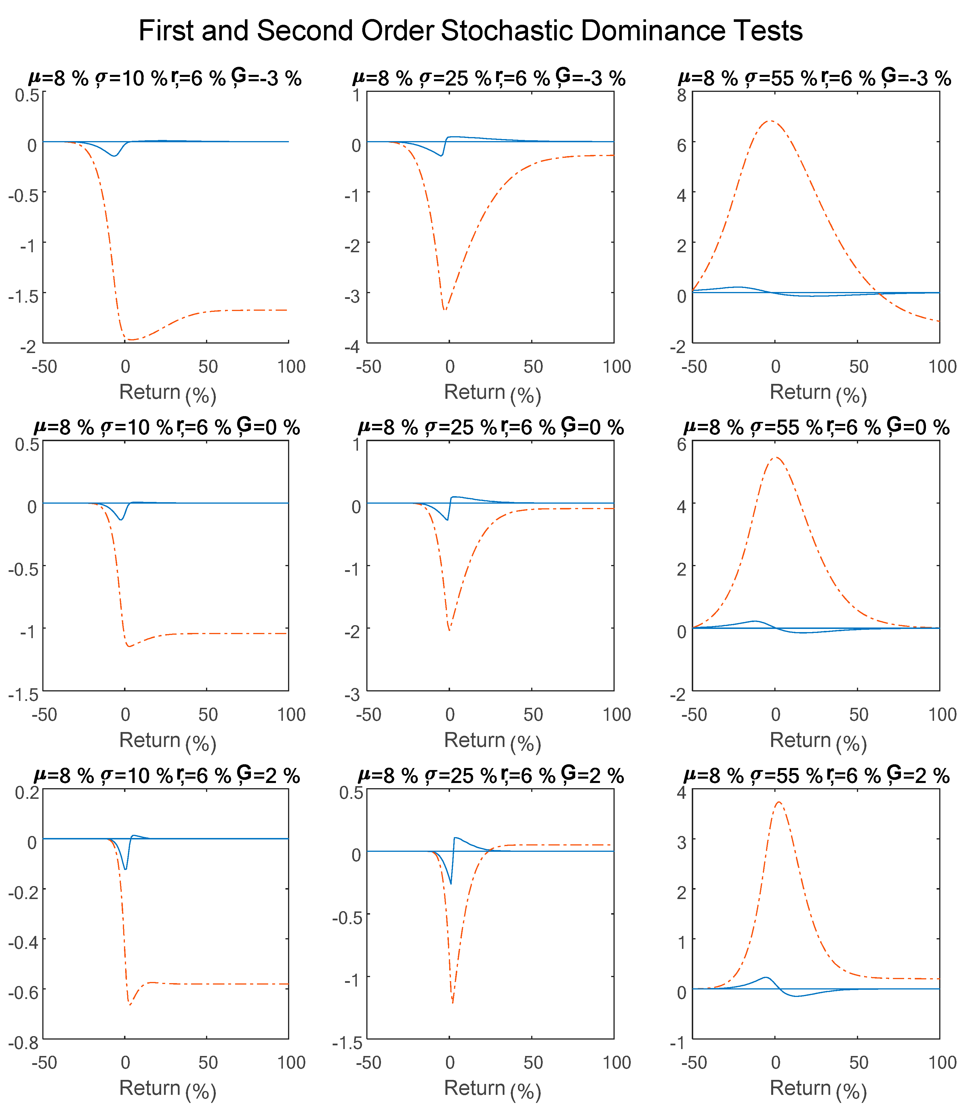
Return versus Risk Analysis

We analyze the returns and the risks of the SP and the managed portfolio returns using several analytical methods, assuming that investors choose investment portfolios that maximize the expected utility of the portfolio. Hence, we use portfolio performance measurements such as average excess return over risk-free interest, the standard deviation of the returns, and the Sharpe ratio, which calculates the ratio between excess return and standard deviation. We also use the Sortino and Price (1994) performance measure, which proposes to reflect the asymmetric distribution of the left tails of these returns. In particular, Sortino and Price (1994) propose to focus on the negative deviations of a portfolio’s returns that fall short of the minimum acceptable return (MAR). Hence, the Sortino ratio calculates the ratio between the average excess return over MAR and the measured standard deviation of sub-MAR returns (downside deviation) by

$$Sortino Ratio=\frac{\overline{R_t-MAR}}{{\sigma }_D}$$

(15)

where the numerator is the average of returns exceeding MAR, and ${\sigma }_D$ is the standard deviation of returns over MAR as calculated by ${\sigma }_D=\sqrt{\frac{1}{N}{\sum }_{t=1}^N{\left({\mathrm{m}\mathrm{i}\mathrm{n}(0,R}_t-MAR)\right)}^2}$.

In this context, studies such as those of Jorion (2001) and Ibragimov and Walden (2007) focus on VaR (value at risk) as an indicator of the risk asymmetry that describes the portfolio loss at a high confidence level (usually 95%). However, given that the VaR indicator does not describe the expected size of the loss, studies such as those of Acerbi and Tasche (2002) and Rockafellar and Uryasev (2002) focus on conditional value at risk (CVaR), the value of which is the average loss below VaR.

To compare the portfolios in our possession, we calculate VaR and CVaR indices as indicators of the risk exposure of the member’s portfolio, as well as the Sharpe ratio and the Sortino ratio, which reflect excess return relative to risk level. We compute them based on the returns of the SP and those of the alternative investment portfolio, which is based on underlying assets. By comparing their values, we can better determine the risk and performance levels of these two different strategies.

4. Results

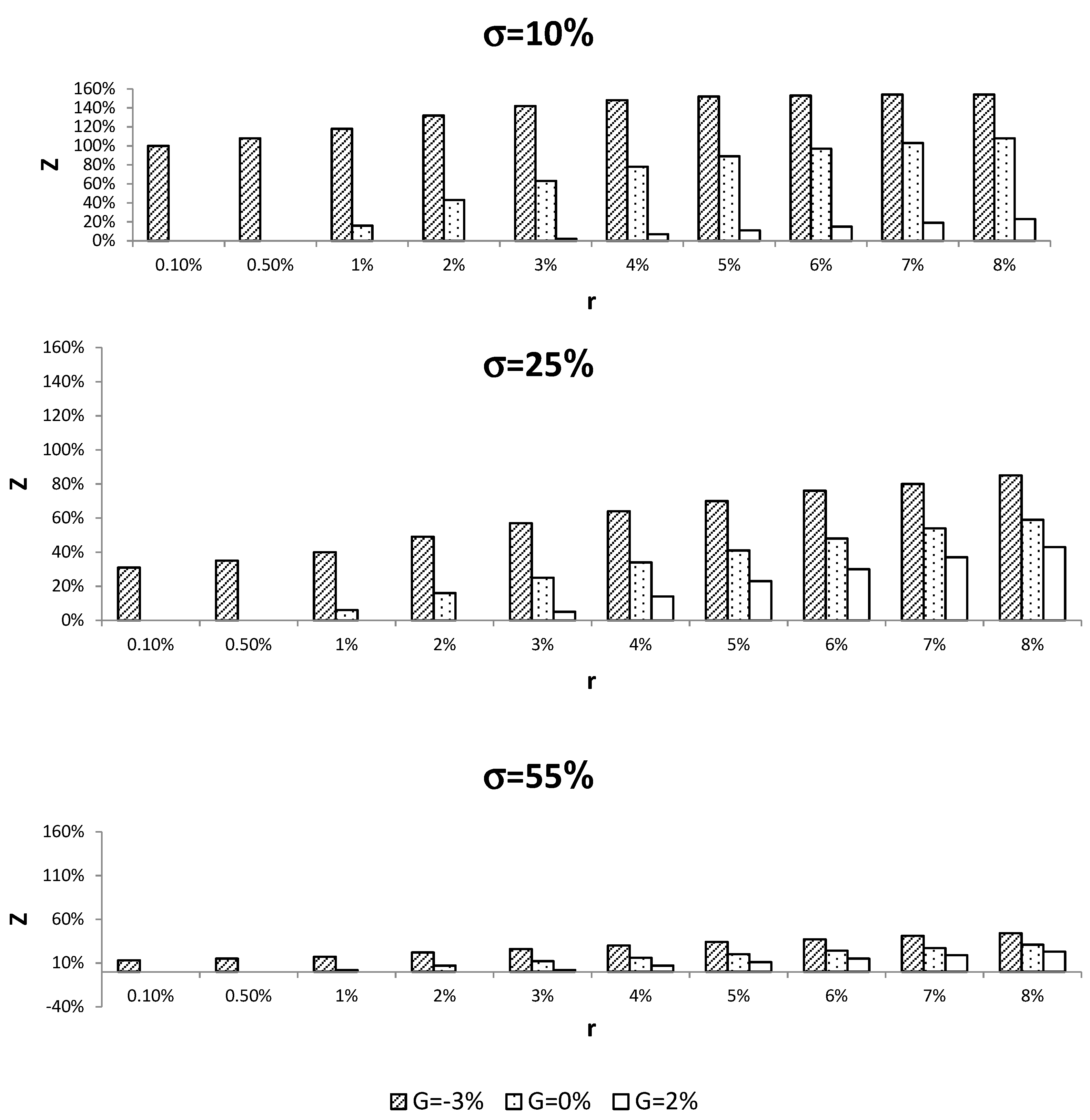
4.1. Sensitivity of Structured Product Characteristics to Market Conditions

The following results show a sensitivity analysis of the characteristics of the SP (Y, Z) as a function of possible risk-free interest rates, the annual standard deviation of the daily return on the benchmark index, and the guaranteed rate of return that the pension member demands.11 Figure 1 shows the maximum Z value of the benchmark return index that the issuer can offer the pension member. The figure displays that value as functions of three different types of guaranteed returns that the pension member demands (G = −3%, 0%, and 2%) and of the risk-free interest rate, r, as they relate to the annual standard deviation, $\sigma$, of the equity market.12 Notably, the SP is unlikely to be issued under high-volatility conditions in the benchmark index because it would be expensive and unattractive. We nonetheless present this scenario to demonstrate both the analysis and the problematic high volatility effect on the SP.

Figure 1 describes Z as a function of the risk-free interest rate and the benchmark index’s standard deviation for three different guaranteed returns. As expected, the results show that settling for a guaranteed rate of return lower than the risk-free interest rate raises the percentage of exposure to the index that the SP can offer the investor. To demonstrate this, assume that r = 3% and $\sigma$ = 10%. In this case, a pension member who wants a guaranteed return of G = 2% will accept a Z = 13% portion of exposure to the benchmark index, in contrast to a pension member who is interested in guaranteeing the principal only (G = 0%), who will accept Z = 63%. The reason for this outcome is that guaranteeing a return that verges on the market free-risk interest results in buying a lower amount of call options (for hedging purposes); therefore, the SP allows only a lower portion of exposure to the benchmark index return.

Figure 1 shows that Z is rather strongly affected by the market’s risk-free interest rate and that a higher portion of the index return can be attained when the risk-free rate rises. The results indicate that in a low-interest-rate environment of 0.1–0.5%, the SP cannot guarantee either a positive 2% return or the pension members’ principal value. Therefore, with a low-interest-rate, pension members interested in buying the SP must settle for protecting only some of their savings. However, the results show that the SP can guarantee payment of the principal if the risk-free interest is higher than 1% and can assure a 2% guaranteed return when the risk-free interest is traded at more than 3%.

Figure 1 also shows that the annual standard deviation of the equity benchmark index has a considerable effect on Z. To demonstrate this, when the risk-free interest rate is r = 4%, the SP offers a pension member who wants principal protection (G = 0%) only a Z = 34% portion of the benchmark index in cases of highly volatile index returns ($\sigma$ = 25%); compare this to Z = 78%, when the index return is relatively stable ($\sigma$ = 10%). The high differences in Z can be attributed to differences in the price of the call option on the benchmark index, which is highly affected by the standard deviation of the index. Therefore, when equity prices are acutely volatile (e.g., the subprime crisis of 2009–2010), the traditional DC pension fund will probably find it difficult to offer investors an SP that guarantees a minimal return. However, in financial turmoil, most investors flee to safety by purchasing high-quality assets (as evident in Longstaff (2004) and Næs et al. (2011)). Despite the relatively low guaranteed return it offers to the investors (with a low percentage of Z), the SP will probably be much in demand.

We also note that the cost of the SP changes as a function of the risk-free rate and the minimal guaranteed return. In other words, pension members who are interested in a guaranteed return that verges on r will pay much less than would pension members who want to ensure a lower guarantee from their portfolios (in return for a higher percentage of exposure to the market return). Accordingly, when the risk-free interest rate rises, investors may be offered a higher guaranteed return with no major change in the cost of the product (see Appendix A).

In sum, the results show that the SP can guarantee a floor value on the accumulated pension savings under various market conditions. Still, the level of the guaranteed return varies largely with the risk-free rate and the volatility of the benchmark index. Specifically, at a risk-free rate above 3%, the SP can provide a good solution for most pension savers, enabling them to profit from a potential upside in the equity market while hedging against a decrease in market value. In particular, in a normal time of low volatility in equity prices, the SP provides a relatively high rate of exposure to the equity market index. Hence, it may be a rather good alternative investment to buy and hold the equity index.

4.2. Simulation Results

The following simulation results describe the performances of pension portfolio returns for a pension member who invests in the SP relative to the return on a balanced investment portfolio that invests Z% in the equity market index and 1 − Z% at the risk-free interest rate. The return is measured from the day the contract is signed to the day on which it expires, and the Monte Carlo simulation settings are set under the same assumptions of (1) a dividend return of q = 3%, (2) an M = 0.5% issuer’s fee, and (3) operating expenses at J = 1% of the issuer’s total hedging cost.

The benchmark index is typified at an annual frequency using geometric Brownian motion across 10,000 simulations, each describing possible changes in the prices of the equity benchmark index for a one-year forward-looking period. Since earlier results showed that the SP could guarantee a return to pension savers when the risk-free rate is above 3%, we chose to exemplify stochastic dominance tests of the SP over the balanced portfolio under this scenario. Hence, we simulate the SP portfolio returns and the balances portfolio by assuming 4% risk-free interest and further assuming that the benchmark equity index has a 4% excess return above the risk-free rate. We justify the risk-free rate assumption with the current risk-free rate derived from the one-year US treasury bill, which traded at around 4.2% (as of March 2023). These settings provide a more realistic basis of our simulation, enabling us to accurately model and analyze the performance of the SP and the balanced portfolio.

Figure 2 shows first- and second-order stochastic dominance tests of the pension portfolio returns attained by the SP relative to the returns attained by the balanced investment portfolio. These tests are based on the difference between the fitted cumulative kernel distribution function (CDF) of the portfolios’ returns (bold line) and the difference between the sum of the CDFs of these returns (dashed line), according to Equations (12) and (13), respectively. By this definition, a negative difference of the CDFs (across the full range of existing returns) indicates the first-order stochastic dominance of the SP over the weighted investment portfolio. In parallel, a negative difference of the sum of the CDFs indicates a second-order stochastic dominance. The figure presents stochastic dominance tests as a function of different rates of guaranteed return (G = −3%, 0%, 2%) and as a function of different risk scenarios of the benchmark equity index ($\sigma$ = 55%, 25%, 10%), where the risk-free interest rate is set to r = 4%, and the expected equity market return is set to $\mu =8\mathrm{\%}$.

Results in Figure 2 do not show first-order stochastic dominance of the SP over the investment portfolio. However, the SP has second-order stochastic dominance over the investment portfolio in certain cases, mostly when the equity market risk is normal. Therefore, when the volatility of the benchmark index is low ($\sigma$ = 10%), the difference of the sum of the CDFs (dashed line) is negative at any possible rate of return, whether the SP guarantees a floor of 97% of the portfolio (G = −3%) or the principal only (G = 0%). Accordingly, in these scenarios, the expected return on the SP exceeds the expected return of the investment portfolio when volatility in the equity market is low.

Figure 2 also shows that no second-order dominance exists when the SP guarantees a G = 2% return. However, when market risk is high, $\sigma$ = 55%, Figure 2 demonstrates that the difference of the CDF is positive, suggesting that the investment portfolio has second-order stochastic dominance over the SP. Nevertheless, such a large standard deviation is usually typical of a crisis in the equity market. Therefore, at such a time, the prices of options on the market will probably be so high as to stop the issuance of these SPs or, at least, make them much less attractive until the market regains a higher degree of stability.

Table 1. Structured product performance compared to a weighted investment portfolio under various volatility scenarios ($\sigma$ = 55%, 25%, 10%) and various guaranteed return rates ($G$ = −3%, 0%, 2%).

Guaranteed Return	Index	σ = 55%		σ = 25%		σ = 10%
		Portfolio	SP	Portfolio	SP	Portfolio	SP
G = −3%	Avg.	0.052	0.0474	0.0669	0.0621	0.1035	0.1067
	S.D.	0.192	0.1486	0.1741	0.1289	0.1593	0.1308
	Sharpe	0.0623	0.050	0.1543	0.1713	0.3984	0.5098
	Sortino	9.8795	22.029	17.9197	62.642	40.124	157.78
	VaR	0.1588	0.03	0.1784	0.03	0.1446	0.03
	CVaR	0.1796	0.03	0.219	0.03	0.1967	0.03
G = 0%	Avg.	0.0463	0.042	0.0541	0.05	0.0734	0.0742
	S.D.	0.1011	0.0806	0.0917	0.07	0.0839	0.071
	Sharpe	0.0623	0.0251	0.1543	0.1426	0.3984	0.4814
	Sortino	12.998	3.5551	22.2919	18.5435	48.755	61.221
	VaR	0.0647	0	0.075	0	0.0572	0
	CVaR	0.0756	0	0.964	0	0.0846	0
G = 2%	Avg.	0.0427	0.0384	0.0461	0.0419	0.0544	0.0525
	S.D.	0.0434	0.0353	0.0394	0.0307	0.036	0.0311
	Sharpe	0.0623	−0.045	0.1543	0.0621	0.3984	0.4021
	Sortino	9.801	−5.915	18.678	6.3166	35.117	31.81
	VaR	0.005	−0.02	0.0094	−0.02	0.0018	−0.02
	CVaR	0.0097	−0.02	0.0186	−0.02	0.0136	−0.02

shows comparative risk and performance measures under various market risks and different guaranteed rates of return. The table also shows the average returns and standard deviations attained by the SP and by the balanced investment portfolio. Included within Table 1 are the portfolio’s risk indicators (VaR and CVaR) and performance indicators (Sharpe, Sortino), obtained from the Monte Carlo simulation. According to the findings in Figure 2, the simulation results show that when the risk level in the market is relatively low ($\sigma$ = 10%), it is almost always better to invest in the SP than in the balanced portfolio. Under these conditions, the SP delivers a higher average return with a lower level of risk (standard deviation) for any given guaranteed return.

To demonstrate that the SP delivers a higher average return with a lower level of risk, the average return on an SP that guarantees the investor’s principal (G = 0%) is 0.0742, compared to 0.0734. At the same time, the standard deviation is much lower (0.071 compared to 0.0839). Using the SP under these circumstances also results in a higher Sharpe ratio (0.481 compared to 0.398) and a higher Sortino ratio (61.22 compared to 48.75), indicating that the SP outperforms the investment portfolio. Furthermore, the VaR obtained by the SP is commensurate with the guaranteed return of the product, which in any case is far below the VaR obtained by the investment portfolio for any guaranteed rate of return. Hence, when the equity market risk is relatively low ($\sigma =10\%$), we find that it is better to invest in the SP than the investment portfolio because the SP results in a higher portfolio return with a lower level of risk. At the same time, the SP also hedges the investor’s portfolio against a sudden loss, as depicted by the 0 (zero) values of the VaR and CVaR measures, compared to respective positive values of the portfolio for any given volatility scenario. These results imply that the SP provides hedging capabilities against market risk.

These findings illustrate that the SP is attractive to average investors, who are primarily interested in increasing their exposure to the market without being exposed to downside risk. Therefore, in our estimation, and under these conditions, the SP will be in demand among pension savers because it promises to concurrently hedge the portfolio and deliver a return that will generally exceed that of an investment portfolio equally exposed to the capital market.

However, when we observe a medium- to high-market-risk level, we find the opposite trend in some cases, where the investment portfolio outperforms the SP. Simulation results show higher Sharpe ratios and Sortino ratios for the investment portfolio compared to the SP for almost all guaranteed rates of return (except for the case of $\sigma =25\%$ and $G=-3\%$), indicating that the balanced investment portfolio outperforms the SP, as reflected in the stochastic dominance tests shown in Figure 2. However, these findings should be treated with caution, particularly in the case of extreme market volatility, with a $\sigma$ = 55%, which occurs mostly at times of financial turmoil in which the falling prices typify the equity market. Thus, in contrast to the simulation results in these cases, we would usually expect to see a lower, if not negative, return. Under these conditions, the SP would likely deliver a higher return than the investment portfolio because it limits the investor’s loss.

These findings are also reflected in a higher Sortino ratio, which shows that at any given level of market volatility, an SP that hedges a loss of up to G = −3% (i.e., provides a floor value of 97%) provides a higher excess return, relative to the downside deviation, than the balances of the investment portfolio. Therefore, in these cases, an SP that provides a guaranteed return would probably be in greater pension member demand than the investment portfolio.

In sum, the results show that under certain market conditions, the SP we have developed may be worthwhile for most types of pension members who want to invest in the equity market and to protect their pension savings. In an interest rate environment of 3% or more and under a low level of risk ($\sigma$ = 10%), the SP is advantageous for pension members who want to protect their pension savings. Furthermore, in cases where the SP gives partial or full hedging of the pension savings portfolio (G = −0.3% and G = 0%, respectively), it has second-order stochastic dominance over the investment portfolio. It gives the pension member a higher return than the balanced investment portfolio at the same level of risk. Under these conditions, because the SP also improves the safety of their investment, we find the SP to be an advantageous financial instrument for the average risk-averse pension member.

However, updated data from the OECD (2021) show that the average short-term interest rate in the Euro area (19 countries) is traded around 2.91% and around 4.91% in the U.S.13 Hence, we realize that under current interest rate conditions, the SP may be a good alternative for individual savers who seek to profit from the equity market while hedging their potential loss. Yet, Figure 1 shows that even with a low interest rate of 0.1% (and under normal market volatility), the SP can still guarantee the investors a floor level for their investment portfolio. Thus, if the interest rate level will get lower than the 2021 level, the SP may also be an attractive alternative investment for those interested in hedging investment risks. However, projections of future interest rates in the near term show no signs for lowering interest rates in the near future in many OECD member states (particularly in the Eurozone); thus, our SP may be a good investment solution for pension fund members who want to protect their portfolios in full.14

5. Summary and Conclusions

The shift from DB to DC pension schemes observed in many OECD countries and an increase in the exposure of DC pension funds to the capital market have increased investment risk to the individual pension saver. This risk is expected to intensify in the future. The shift to DC pension schemes is expected to grow in many OECD countries (OECD 2016), while more and more DC pension funds allocate their holdings towards more risky assets traded in capital markets (OECD 2020). While investment in capital markets may increase the individual’s accumulated pension savings, it may prove burdensome to risk-averse individuals. This burden is particularly true for those nearing retirement, who mostly seek a haven for their accumulated pension savings (through investment in tradable government bonds).

The SP presented herein enables DC pension funds to satisfy individuals’ demand for a guaranteed floor for their accumulated savings while investing it in the capital market. Hence, it may be a better financial alternative to individual savers. Simulation results under normal equity market conditions (i.e., with relatively low standard deviation and higher risk-free rate) show that the SP can generate average returns better than those achieved by direct equity market investing (with equivalent asset allocation) and with a lower level of risk. Accordingly, we conclude that under these conditions, the SP is a better investment alternative for the individual pension saver because it offers a less risky and more profitable investment than a portfolio managed by the DC pension fund.

In this context, the SP’s competitive advantage to the individual pension saver results in a higher competitive advantage to the DC pension fund (among other players in the pension market), particularly when DC funds can define the SP under changing market conditions. Hence, while DC pension schemes become less attractive among pension savers (Antolín et al. 2011), marketing the SP by DC pension funds may significantly increase their popularity and bring a major change in pension markets among OECD member states.

References

1. Acerbi, Carlo, and Dirk Tasche. 2002. On the coherence of expected shortfall. Journal of Banking and Finance 26: 1487–503. [Google Scholar] [CrossRef] [Green Version]
2. Antolín, Pablo, Stéphanie Payet, Edward Whitehouse, and Juan Yermo. 2011. The Role of Guarantees in Defined Contribution Pensions, OECD Working Papers on Finance, Insurance and Private Pensions, No. 11. Paris: OECD Publishing. [Google Scholar] [CrossRef]
3. Bateman, Hazel, Christine Eckert, Fedor Iskhakov, Jordan Louviere, Stephen Satchell, and Susan Thorp. 2018. Individual capability and effort in retirement benefit choice. Journal of Risk and Insurance 85: 483–512. [Google Scholar] [CrossRef]
4. Benartzi, Shlomo, and Richard Thaler. 2001. Naive diversification strategies in defined contribution saving plans. American Economic Review 91: 79–98. [Google Scholar] [CrossRef] [Green Version]
5. Black, Fisher, and Miron Scholes. 1973. The pricing of options and corporate liabilities. The Journal of Political Economy 81: 637–54. [Google Scholar] [CrossRef] [Green Version]
6. Bodie, Zvi, and Dwight Crane. 1999. The design and production of new retirement savings products. Journal of Portfolio Management 25: 77–82. [Google Scholar] [CrossRef]
7. Broadbent, John, Michael Palumbo, and Elizabeth Woodman. 2006. The Shift from Defined Benefit to Defined Contribution Pension Plans–Implications for Asset Allocation and Risk Management. Sydeny: Reserve Bank of Australia, Board of Governors of the Federal Reserve System and Bank of Canada. [Google Scholar]
8. Célérier, Clair, and Boris Vallée. 2017. Catering to investors through security design: Headline rate and complexity. The Quarterly Journal of Economics 132: 1469–508. [Google Scholar] [CrossRef]
9. Clark, Gordon, and Tessa Hebb. 2004. Pension fund corporate engagement: The fifth stage of capitalism. Relations Industrielles/Industrial Relations 59: 142–71. [Google Scholar] [CrossRef] [Green Version]
10. Dichtl, Hubert, and Wolfgang Drobetz. 2011. Portfolio insurance and prospect theory investors: Popularity and optimal design of capital protected financial products. Journal of Banking and Finance 35: 1683–97. [Google Scholar] [CrossRef]
11. Dimitrov, Stanislav, and Elroi Hadad. 2022. Pension tracking system application: A new supervision challenge in the EU. International Journal of Economic Sciences XI: 48–57. [Google Scholar] [CrossRef]
12. European Commission. 2021. The 2021 Pension Adequacy Report. Luxembourg: Publications Office of the European Union, vol. 2. [Google Scholar]
13. Fang, Hanming. 2016. Insurance markets for the elderly. Handbook of the Economics of Population Aging 1: 237–309. [Google Scholar]
14. Gustman, Alan, and Thomas Steinmeier. 1992. The stampede toward defined contribution pension plans: Fact or fiction? Industrial Relations: A Journal of Economy and Society 31: 361–69. [Google Scholar] [CrossRef] [Green Version]
15. Hadad, Elroi, Stanislav Dimitrov, and Jivka Stoilova-Nikolova. 2022. Development of capital pension funds in the Czech Republic and Bulgaria and readiness to implement PEPP. European Journal of Social Security 24: 342–60. [Google Scholar] [CrossRef]
16. Hadar, Josef, and William Russell. 1969. Rules for ordering uncertain prospects. The American Economic Review 59: 25–34. [Google Scholar]
17. Hens, Thorsten, and Marc Oliver Rieger. 2014. Can utility optimization explain the demand for structured investment products? Quantitative Finance 14: 673–81. [Google Scholar] [CrossRef] [Green Version]
18. Hull, John. 2012. Options, Futures, and Other Derivatives, 8th ed. Chennai: Pearson Education India. [Google Scholar]
19. Ibragimov, Rustam, and Johan Walden. 2007. The limits of diversification when losses may be large. Journal of Banking and Finance 31: 2551–69. [Google Scholar] [CrossRef] [Green Version]
20. Jorion, Philippe. 2001. Value at Risk: The New Benchmark for Controlling Market Risk. New York: McGraw-Hill. [Google Scholar]
21. Knoller, Christian. 2016. Multiple Reference Points and the Demand for Principal-Protected Life Annuities: An Experimental Analysis. Journal of Risk and Insurance 83: 163–79. [Google Scholar] [CrossRef]
22. Lachance, Marie-Eve, Olivia Mitchell, and Kent Smetters. 2003. Guaranteeing defined contribution pensions: The option to buy back a defined benefit promise. Journal of Risk and Insurance 70: 1–16. [Google Scholar] [CrossRef] [Green Version]
23. Longstaff, Francis. 2004. The flight-to-liquidity premium in U.S. Treasury bond prices. Journal of Business 77: 511–26. [Google Scholar] [CrossRef] [Green Version]
24. Mohammadi, Arezoo, Mehrzad Minnoei, Zadollah Fathi, Mohamamd Ali Keramati, and Hossein Baktiari. 2022. Optimal allocation of bank resources and risk reduction through portfolio decentralization. International Journal of Economic Sciences 11: 92–143. [Google Scholar] [CrossRef]
25. Næs, Randi, Johannes Skjeltorp, and Bent Arne Ødegaard. 2011. Stock market liquidity and the business cycle. The Journal of Finance 66: 139–76. [Google Scholar] [CrossRef]
26. OECD. 2016. OECD Pensions Outlook 2016. Paris: OECD Publishing. [Google Scholar]
27. OECD. 2020. OECD Pensions Markets in Focus. 2020. Paris: OECD Publishing. [Google Scholar]
28. OECD. 2021. Short-Term Interest Rates (Indicator). Available online: https://www.oecd-ilibrary.org/finance-and-investment/short-term-interest-rates/indicator/english_2cc37d77-en (accessed on 26 October 2022).
29. Quirk, James, and Rubin Saposnik. 1962. Admissibility and measurable utility functions. The Review of Economic Studies 29: 140–46. [Google Scholar] [CrossRef]
30. Randle, Tony, and Heinz Rudolph. 2014. Pension Risk and Risk-Based Supervision in Defined Contribution Pension Funds. World Bank Policy Research Working Paper 6813. Washington: The World Bank. [Google Scholar]
31. Rockafellar, Tyrrel, and Stanislav Uryasev. 2002. Conditional value-at-risk for general loss distributions. Journal of Banking and Finance 26: 1443–71. [Google Scholar] [CrossRef]
32. Sortino, Frank, and Lee Price. 1994. Performance measurement in a downside risk framework. Journal of Investing 3: 50–8. [Google Scholar] [CrossRef]
33. Thomas, Ashok, Luka Spataro, and Nanditha Mathew. 2014. Pension funds and stock market volatility: An empirical analysis of OECD countries. Journal of Financial Stability 11: 92–103. [Google Scholar] [CrossRef] [Green Version]
34. Whitehouse, Edward. 2007. Life-Expectancy Risk And Pensions: Who Bears The Burden? Paris: Organisation for Economic Cooperation and Development (OECD). Available online: https://www.proquest.com/docview/189843487?accountid=27473&forcedol=true (accessed on 26 October 2022).
35. Yosef, Rami. 2006. Floor Options on Structured Products and Life Insurance Contracts. Investment Management and Financial Innovations 3: 160–70. [Google Scholar]
Figure 1. The maximum portion (Z, in pct.) of the benchmark index return that the SP can offer to the investor as a function of the risk-free interest rate and the standard deviation of the benchmark index’s returns.
Risks 11 00107 g001
Figure 2. First- and second-order stochastic dominance tests of pension portfolio returns attained by the SP, compared to the returns of a portfolio attained by buying Z% of the benchmark index and a 1-Z% risk-free rate (to an investment term of one year ahead).
Risks 11 00107 g002