Interleaving Shifted Versions of a PN-Sequence

Abstract

The output sequence of the shrinking generator can be considered as an interleaving of determined shifted versions of a single PN -sequence. In this paper, we present a study of the interleaving of a PN-sequence and shifted versions of itself. We analyze some important cryptographic properties as the period and the linear complexity in terms of the shifts. Furthermore, we determine the total number of the interleaving sequences that achieve each possible value of the linear complexity.

1. Introduction

Stream ciphers are fast encryption algorithms since they consist of applying a bit-wise XOR operation among the bits of the keystream sequence and the message to obtain the ciphertext. The same bit-wise XOR operation between the ciphertext and the keystream is done to recover the original message.

Many keystream generators are based on maximal-length Linear Feedback Shift Registers (LFSRs) [1] because they offer several advantages due to their performance. They also have an easy hardware and software implementation in cryptographic applications. For example, some widely used stream ciphers based on LFSRs are the cryptosystem E0 for Bluetooth [2], the A5/1 for GSM use [3], or the SNOW 2.0 used in UMTS 3G networks [4].

The output sequences of a maximal-length LFSR, whose characteristic polynomial is primitive, are called PN -sequences [5]. These sequences have the largest period and present good randomness properties as balancedness, large period, low correlation, excellent runs distribution, and so forth. However, they are easily predictable due to their inherent linearity. In order to break this linearity, but at the same time maintaining the pseudorandomness characteristics, different design techniques are applied—non-linear filtering, combinational generators, clock-controlled generators or the irregular decimation of PN-sequences, among others.

We focus our attention on a particular kind of stream ciphers based on LFSRs where an irregular decimation is applied: the class of shrinking generators [6,7,8,9,10]. The shrinking generator is a pseudorandom number generator based on a simple combination of two LFSRs which are clocked synchronously [7]. Its simplicity and efficiency of implementation, in addition to the generation of sequences with good cryptographic properties, make it suitable for its real use in stream cipher cryptosystems. For example, the shrinking generator is part of the internal structure of different stream ciphers as the EP0619659A2 [11], an European patent application; or the Decim${}^{v_2}$, a hardware oriented stream cipher submitted to the ECRYPT Stream CipherProject (eSTREAM) [12], among other applications [6,13].

From the shrinking generator emerged a great family of decimation-based sequence generators, which are improved versions of this or themselves—the self-shrinking generator [10], the generalized self-shrinking generator [8], the modified self-shrinking generator [9] and the t-modified self-shrinking generator [14]; there exists a complete guide in [6] that offers a thorough study of all these generators, their fundamentals and applications. These generators are fast, easy and with low implementation costs to generate good cryptographic sequences. The authors of [15] presented a statistical and graphical study of the randomness of the sequences generated by the generalized self-shrinking generator that prove their suitability for cryptographic applications.

The output sequences of a shrinking generator, called shrunken sequences, have been widely studied in several mathematical fields in the last decades. For instance, they have been considered particular solutions of a kind of linear difference equations [16,17]; they have also been studied as the output sequences of linear elementary cellular automata (CA) [18]. Furthermore, the shrunken sequences can be expressed as the interleaving of shifted versions of a PN-sequence [19,20]. In [18], the authors determined how to compute the shifts of the interleaved sequences that compose the shrunken sequence. This fact can be used advantageously to design cryptanalytic attacks against this generator [18,21,22,23,24]. A natural way to deal with this vulnerability is to alter the shifts or interleave PN-sequences of different primitive polynomials. In this paper, we study the resultant sequences of interleaving shifted versions of the same PN-sequence with different shifts. We analyze the conditions that must satisfy these shifts to obtain interleaving sequences with high linear complexity and long period.

In Section 2, we introduce some preliminary concepts and results about the shrinking generator; we define the main concept of interleaving sequence and we check that the shrunken sequence can be expressed as an interleaving of PN-sequences. In Section 3, we analyze the period and the linear complexity of the resultant sequences of interleaving $2^t$ shifted versions of a given PN-sequence. We study, in depth, the cases of 2 and 4 interleaving sequences obtaining the amount of them which have certain values for linear complexity. In Section 4, we give some preliminary results about the case of interleaving t PN-sequences. In Section 6, we present the main conclusions of our research and the future work.

2. Interleaving Sequences in the Shrinking Generator

First of all, we recall the concept of decimation. The decimation of a sequence ${\left\{v_i\right\}}_{i\ge 0}$ by d is a new sequence obtained by taking every d-th term of ${\left\{v_i\right\}}_{i\ge 0}$, that is, ${\left\{v_{d·i}\right\}}_{i\ge 0}$ [25].

Let ${\mathbb{F}}_2$ be the Galois field of two elements. In this section, we consider two maximal-length LFSRs, $R_1$ and $R_2$, with characteristic polynomials $p_1\left(x\right),p_2\left(x\right)\in {\mathbb{F}}_2\left[x\right]$, lengths $L_1$ and $L_2$ with $L_1<L_2$ and $gcd(L_1,L_2)=1$, and $T_1=2^{L_1}-1$ and $T_2=2^{L_2}-1$ the periods of the corresponding PN-sequences, respectively. Besides, the PN-sequences generated by both registers are ${\left\{a_i\right\}}_{i\ge 0}$ and ${\left\{b_i\right\}}_{i\ge 0}$, respectively, with $a_i,b_i\in {\mathbb{F}}_2$. From now on, we denote any sequence ${\left\{v_i\right\}}_{i\ge 0}$ by $\left\{v_i\right\}$, without loss of generality.

The shrinking generator [7] is composed of two maximal-length LFSRs, $R_1$ and $R_2$, with the properties mentioned before. The PN-sequence $\left\{a_i\right\}$ generated by $R_1$ decimates the PN-sequence $\left\{b_i\right\}$ produced by $R_2$. The decimation rule is very simple—given two bits $a_i$ and $b_i$, for $i=0,1,2,\dots$, of both PN-sequences, the output sequence $\left\{s_j\right\}$ is obtained as follows:

$$\left\{\begin{array}{c}\mathrm{If}{a}_i=1,\mathrm{then}{s}_j=b_i.\hfill \\ \mathrm{If}{a}_i=0,\mathrm{then}{b}_i\mathrm{is}\mathrm{discarded}.\hfill \end{array}\right.$$

The sequence $\left\{s_j\right\}$ is called the shrunken sequence and its period is $T=(2^{L_2}-1)2^{L_1-1}$. The linear complexity of this sequence, denoted by $LC$, satisfies $L_2{2}^{L_1-2}<LC\le L_2{2}^{L_1-1}$ and its characteristic polynomial has the form $p{\left(x\right)}^m$, where $2^{L_1-2}<m\le 2^{L_1-1}$ and $p\left(x\right)$ is a primitive polynomial of degree $L_2$ [26].

Notice that the shrunken sequence is obtained by irregular decimation of a PN-sequence, as we can see in the following example.

Example 1.

Consider $R_1$ the LFSR with characteristic polynomial $p_1\left(x\right)=1+x+x^2$ and initial state $\left\{11\right\}$. Consider also $R_2$ the LFSR with characteristic polynomial $p_2\left(x\right)=1+x^2+x^3$ and initial state $\left\{111\right\}$. The shrunken sequence can be computed in the following way:

$$\begin{array}{cccccccccccccccccccccc}{R}_1:& 1& 1& 0& 1& 1& 0& 1& 1& 0& 1& 1& 0& 1& 1& 0& 1& 1& 0& 1& 1& 0\\ R_2:& 1& 1& \xcancel{1}& 0& 1& \xcancel{0}& 0& 1& \xcancel{1}& 1& 0& \xcancel{1}& 0& 0& \xcancel{1}& 1& 1& \xcancel{0}& 1& 0& \xcancel{0}\\ \left\{s_j\right\}:& \mathbf{1}& \mathbf{1}& & \mathbf{0}& \mathbf{1}& & \mathbf{0}& \mathbf{1}& & \mathbf{1}& \mathbf{0}& & \mathbf{0}& \mathbf{1}& & \mathbf{1}& \mathbf{1}& & \mathbf{1}& \mathbf{0}.& \end{array}$$

The sequence has period 14 and it is not difficult to check that its characteristic polynomial is $p{\left(x\right)}^2={(1+x+x^3)}^2$, consequently its linear complexity is 6.

It is worth mentioning that all the results that appear in this work are valid for large values of L, where L is the length of the LFSR that generates the corresponding PN-sequences in each case. We use small examples in order to illustrate the ideas. In practical applications, the recommended values in the shrinking case are $L_1,L_2\ge 64$, so the key has at least 128 bits.

The following definition introduces one of the main concepts of this paper.

Definition 1.

We say that the sequence $\left\{s_j\right\}$ is obtained interleaving the sequences $\left\{u_i^{\left(1\right)}\right\}$, $\left\{u_i^{\left(2\right)}\right\}$, …, $\left\{u_i^{\left(t\right)}\right\}$, all of them of period T, if it has the following form:

$$\left\{s_j\right\}=\left\{u_0^{\left(1\right)},u_0^{\left(2\right)},\dots ,u_0^{\left(t\right)},u_1^{\left(1\right)},u_1^{\left(2\right)},\dots ,u_1^{\left(t\right)},\dots ,u_{T-1}^{\left(1\right)},u_{T-1}^{\left(2\right)},\dots ,u_{T-1}^{\left(t\right)}\right\}.$$

We call this sequence a t-interleaving sequence.

From now on, we always consider that these t sequences $\left\{u_i^{\left(j\right)}\right\}$ for $j=1,2,\dots ,t$, are (left circular) shifted versions of a given PN-sequence $\left\{u_i\right\}$. Notice that, in this case, if the characteristic polynomial $p\left(x\right)$ of $\left\{u_i\right\}$ is a primitive polynomial of degree L, then the resultant t-interleaving sequence is almost balanced as its number of 1s is $t·2^{(L-1)}$.

The following result shows us that the shrunken sequence is an $\left(2^{L_1-1}\right)$-interleaving sequence.

Theorem 1

([27] Theorem 3.1).The sequences obtained decimating by (distance) $2^{L_1-1}$ the shrunken-sequence are PN-sequences with period $T_2$. We call these sequences the interleaved PN-sequences of the shrunken sequence.

It is worth noticing that the $2^{L_1-1}$ interleaved PN-sequences of the shrunken sequence correspond to shifted versions of the same PN-sequence. The following example illustrate the previous results.

Example 2.

Consider $R_1$ the LFSR with characteristic polynomial $p_1\left(x\right)=1+x^2+x^3$, $L_1=3$ and initial state $\left\{111\right\}$. The corresponding PN-sequence has period $T_1=7$. Consider also $R_2$ the LFSR with characteristic polynomial $p_2\left(x\right)=1+x^3+x^4,L_2=4$ and initial state $\left\{1111\right\}$. The corresponding PN-sequence has period $T_2=15$. The shrunken-sequence is given by:

$$\left\{s_j\right\}=\left\{111011010111011000111010000101011001101101001100001011111000\right\}$$

This sequence has period $T=(2^{L_2}-1)2^{L_1-1}=60$ and it is possible to check that the characteristic polynomial is $p{\left(x\right)}^{16}={(1+x+x^4)}^4$, this is, $LC=16$. If we decimate the shrunken sequence by (distance) $d=2^{L_1-1}=4$, we obtain 4 PN-sequences:

$$\begin{array}{cc}\hfill \left\{s_{4·j}\right\}:& 110001001101011\hfill \\ \hfill \left\{s_{4·j+1}\right\}:& 111100010011010\hfill \\ \hfill \left\{s_{4·j+2}\right\}:& 101111000100110\hfill \\ \hfill \left\{s_{4·j+3}\right\}:& 011010111100010\hfill \end{array}$$

Notice that the characteristic polynomial of the four PN-sequences is $p\left(x\right)=1+x+x^4$ (the reciprocal polynomial of $p_2\left(x\right)$), that is, the four PN-sequences are shifted versions of the same sequence.

The next theorem shows us how to obtain the characteristic polynomial of the interleaved PN-sequences.

Theorem 2

([27] Theorem 3.3).The primitive polynomial $p\left(x\right)$ that generates the interleaved PN-sequences of the shrunken sequence can be computed as

$$p\left(x\right)=\left(x+{\alpha }^{T_1}\right)\left(x+{\alpha }^{2T_1}\right)\left(x+{\alpha }^{4T_1}\right)\cdots \left(x+{\alpha }^{2^{L_2-1}{T}_1}\right),$$

where $\alpha \in {\mathbb{F}}_{2^{L_2}}$ is root of $p_2\left(x\right)$. If $L_2=L_1+1$, then the polynomial $p\left(x\right)$ is the reciprocal polynomial of $p_2\left(x\right)$.

Note that the characteristic polynomial of the shrunken sequence is $p{\left(x\right)}^m$, and $p\left(x\right)$ only depends on $p_2\left(x\right)$. The polynomial $p_1\left(x\right)$ only affects to the power m. In this way, given a fixed polynomial $p_2\left(x\right)$, every primitive polynomial with degree $L_1$ would provide the same $p\left(x\right)$.

Example 3.

Consider again Example 2. Notice that

$$p\left(x\right)=\left(x+{\alpha }^7\right)\left(x+{\alpha }^{14}\right)\left(x+{\alpha }^{28}\right)\left(x+{\alpha }^{56}\right)=1+x+x^4,$$

where $\alpha \in {\mathbb{F}}_{2^4}$ is root of $p_2\left(x\right)=1+x^3+x^4$. Observe that $p\left(x\right)$ is the reciprocal polynomial of $p_2\left(x\right)$.

It is worth noticing that if $p\left(x\right)$ is the primitive polynomial that generates the interleaved PN-sequences of the shrunken sequence, then the polynomial $p{\left(x\right)}^{2^{L_1-1}}$ also generates the shrunken sequence. However, this polynomial might not be the characteristic polynomial. In some cases, the characteristic polynomial has the form $p{\left(x\right)}^m$, with $2^{L_1-2}<m<2^{L_1-1}$.

The interleaved PN-sequences of the shrunken sequence are shifted versions of the same PN-sequence, and these shifts can be determined [18]. Denote each one of the $2^{L_1-1}$ interleaved PN-sequences by:

$$\left\{v_i\right\},\left\{v_{i+d_1}\right\},\left\{v_{i+d_2}\right\},\dots ,\left\{v_{i+d_{2^{L_1-1}-1}}\right\}.$$

The shifts $d_j$, with $j=1,2,3,\dots ,2^{L_1-1}-1$, depend on the positions of the ones in the PN-sequence $\left\{a_i\right\}$ generated by $p_1\left(x\right)$ in the shrinking process. The following theorem gives us a way to compute these shifts.

Theorem 3

([18] Proposition 2).Let $\delta \in \{1,2,3,\dots ,T_2-1\}$, such that $T_1·\delta =1mod{T}_2$. Denote by $I=\{0,i_1,i_2,\dots ,i_{2^{L_1-1}-1}\}$ the set of positions of the 1s in the PN-sequence $\left\{a_i\right\}$ generated by $p_1\left(x\right)$ in its first period. We have that

$$d_j=\delta ·i_{j}mod{T}_2,j=1,2,\dots ,2^{L_1-1}-1.$$

Example 4.

Consider again Example 2. We have that the interleaved sequences of the shrunken sequence are:

$$\begin{array}{cc}\hfill \left\{s_{4·j}\right\}:& 110001001101011\hfill \\ \hfill \left\{s_{4·j+1}\right\}:& 111100010011010\hfill \\ \hfill \left\{s_{4·j+2}\right\}:& 101111000100110\hfill \\ \hfill \left\{s_{4·j+3}\right\}:& 011010111100010\hfill \end{array}$$

The four PN-sequences $\left\{s_{4·j+i}\right\}$, for $i=0,1,2,3$, have the same characteristic polynomial $p\left(x\right)=1+x+x^4$, thus all of them are shifted versions of the same PN-sequence. We can rename them as:

$$\begin{array}{cc}\hfill \left\{v_i\right\}:& 1100010\overline{0}110\mathbf{1}0\underline{1}1\hfill \\ \hfill \left\{v_{i+d_1}\right\}:& \underline{1}11100010011010\hfill \\ \hfill \left\{v_{i+d_2}\right\}:& \mathbf{1}01111000100110\hfill \\ \hfill \left\{v_{i+d_3}\right\}:& \overline{0}11010111100010\hfill \end{array}$$

(1)

We consider, without loss of generality, that the last three PN-sequences are shifted versions of the first one. From Theorem 3, we know that these shifts $d_j$, for $j=1,2,3$, depend on the ones in the PN-sequence $\left\{a_i\right\}$ generated by $p_1\left(x\right)=1+x^2+x^3$ in the shrinking process. In order to obtain these values, we have to find a value δ such that $7·\delta =1mod15$. In this case, $\delta =13$. Now, we know that the ones in $\left\{a_i\right\}$ are in the positions $\{0,1,2,4\}$, thus:

$$\begin{array}{cc}\hfill d_1& =13·1mod15\to d_1=13\hfill \\ \hfill d_2& =13·2mod15\to d_2=11\hfill \\ \hfill d_3& =13·4mod15\to d_3=7\hfill \end{array}$$

and, therefore, $\left\{a_i\right\}=\left\{1110100\right\}.$

It is easy to check (see Equation (1)) that the second PN-sequence $\left\{v_{i+d_1}\right\}$ starts in the 13-th position of the first PN-sequence $\left\{v_i\right\}$ (underlined bit), the third $\left\{v_{i+d_2}\right\}$ in the 11-th position (bit in bold) and the last one $\left\{v_{i+d_3}\right\}$ in the 7-th position (overlined bit).

The weakness of the shrunken sequence lies in the fact that the shifts of the interleaved sequences can be determined. This means that, a shrunken sequence cannot be obtained from some random shifted versions of a given PN-sequence; on the contrary, the shifts are known as we saw before. In this fact our research begins.

3. Interleaving ${\mathbf{2}}^{\mathit{t}}$ Shifted Versions of the Same PN-Sequence

In this section, we study the resultant sequences of interleaving any shifted versions of the same PN-sequence, that is, the so-called t-interleaving sequences. We determine certain conditions on the shifts in order to obtain interleaving sequences with high linear complexity, long period and good cryptographic properties.

In the following subsections, we analyze the cases of interleaving 2 and 4 shifted versions of a same PN-sequence with a view to establish general conditions for the $2^t$ PN-sequences case.

3.1. Analysis of 2-Interleaving Sequences

Consider a primitive polynomial $p\left(x\right)$ of degree L. If we interleave two shifted versions of the same PN-sequence of period $T=2^L-1$, then the period of the resultant 2-interleaving sequence, denoted by $\mathcal{T}$, must be a divisor of $2T$. Our main interest lies in the study of its linear complexity $LC$, since a large linear complexity it is an important cryptographic property in order to resist against cryptanalytic attacks.

By means of the following theorem we can narrow down the possible values of $LC$ for the 2-interleaving sequences.

Lemma 1.

If we interleave two shifted versions of the same PN-sequence generated by the primitive polynomial $p\left(x\right)$, then the resultant 2-interleaving sequence can be generated by $p{\left(x\right)}^2$.

Proof. 

Assume that we have the PN-sequence $\left\{a_i\right\}$ with characteristic polynomial

$$p\left(x\right)=p_0+p_{1}x+p_2{x}^2+\cdots +p_{L-1}{x}^{L-1}+x^L;$$

this means that the PN-sequence $\left\{a_i\right\}$ satisfies the linear recurrence relation:

$$a_{i+L}=p_0{a}_i+p_1{a}_{i+1}+p_2{a}_{i+2}+\cdots +p_{L-1}{a}_{i+L-1}.$$

(2)

Consider now a shifted version of $\left\{a_i\right\}$:

$$\left\{a_{i+k}\right\}=\left\{a_k,a_{k+1},\dots ,a_{k+2^L-2}\right\}.$$

We know that the PN-sequence $\left\{a_{i+k}\right\}$ also satisfies the linear recurrence relation (2) and the sequence obtained by interleaving $\left\{a_i\right\}$ and $\left\{a_{i+k}\right\}$ has the following form:

$$\left\{s_j\right\}=\{a_0,a_k,a_1,a_{k+1},a_2,a_{k+2},\dots \}.$$

Denote the two PN-sequences as $\left\{u_i\right\}=\left\{a_i\right\}$ and $\left\{v_i\right\}=\left\{a_{i+k}\right\}$, for $i=0,1,\dots$, $2^L-2$. We know that

$$\begin{array}{cc}\hfill u_{i+L}& =p_0{u}_i+p_1{u}_{i+1}+p_2{u}_{i+2}+\cdots +p_{L-1}{u}_{i+L-1}\hfill \\ \hfill v_{i+L}& =p_0{v}_i+p_1{v}_{i+1}+p_2{v}_{i+2}+\cdots +p_{L-1}{v}_{i+L-1}\hfill \end{array}$$

(3)

and

$$\begin{array}{cc}\hfill u_i& =a_i=s_{2i}\hfill \\ \hfill v_i& =a_{i+k}=s_{2i+1}.\hfill \end{array}$$

If we substitute the corresponding bits of $\left\{s_j\right\}$ in (3), we have that:

$$\begin{array}{cc}\hfill s_{2i+2L}& =p_0{s}_{2i}+p_1{s}_{2i+2}+p_2{s}_{2i+4}+\cdots +p_{L-1}{s}_{2i+2L-2}\hfill \\ \hfill s_{2i+2L+1}& =p_0{s}_{2i+1}+p_1{s}_{2i+3}+p_2{s}_{2i+5}+\cdots +p_{L-1}{s}_{2i+2L-1}.\hfill \end{array}$$

Now, if we substitute $j=2i$, we have that:

$$\begin{array}{cc}\hfill s_{j+2L}& =p_0{s}_j+p_1{s}_{j+2}+p_2{s}_{j+4}+\cdots +p_{L-1}{s}_{j+2L-2}\hfill \\ \hfill s_{j+2L+1}& =p_0{s}_{j+1}+p_1{s}_{j+3}+p_2{s}_{j+5}+\cdots +p_{L-1}{s}_{j+2L-1}.\hfill \end{array}$$

This means that $\left\{s_j\right\}$ satisfies the linear recurrence relation:

$$s_{j+2L}=p_0{s}_j+p_1{s}_{j+2}+p_2{s}_{j+4}+\cdots +p_{L-1}{s}_{j+2L-2}$$

and, thus,

$$p{\left(x\right)}^2=p_0+p_1{x}^2+p_2{x}^4+\cdots +p_{L-1}{x}^{2(L-1)}+x^{2L}$$

generates the sequence $\left\{s_j\right\}$.  □

Notice that if $p{\left(x\right)}^2$ generates the 2-interleaving sequence, then its characteristic polynomial must be $p{\left(x\right)}^2$ or $p\left(x\right)$. Thus, the linear complexity of the sequence must be $LC=2L$ or $LC=L$, respectively. Moreover, the total number of 2-interleaving sequences, using different shifts, is $T^2$.

The following theorem shows that, given a PN-sequence $\left\{a_i\right\}$ and a shifted version of itself with shift $k\ne 2^{L-1}$, the characteristic polynomial of the 2-interleaving sequence $\left\{s_j\right\}$ cannot be the same characteristic polynomial as that of $\left\{a_i\right\}$. In other words, the shift $k=2^{L-1}$ is the only shift that produces a 2-interleaving sequence with $LC=L$.

Theorem 4.

Consider the PN-sequence $\left\{a_i\right\}$ generated by a primitive polynomial $p\left(x\right)$ of degree L and $\left\{a_{i+k}\right\}$ a version of $\left\{a_i\right\}$ shifted k positions. If $k\ne 2^{L-1}$, then the resultant 2-interleaving sequence $\left\{s_j\right\}$ cannot be the PN-sequence $\left\{a_i\right\}$ neither a shifted version of it.

Proof. 

Consider the PN-sequences:

$$\begin{array}{ccccccc}\hfill \left\{a_i\right\}:& a_0\hfill & a_1\hfill & a_2\hfill & a_3\hfill & \dots \hfill & a_{2^L-2}\hfill \\ \hfill \left\{a_{i+k}\right\}:& a_k\hfill & a_{k+1}\hfill & a_{k+2}\hfill & a_{k+3}\hfill & \dots \hfill & a_{k+2^L-2}\hfill \end{array}$$

and the resultant 2-interleaving sequence

$$\left\{s_j\right\}=\left\{a_0,a_k,a_1,a_{k+1},a_2,a_{k+2},\dots ,a_{2^L-2},a_{k+2^L-2},\right\}$$

with period divisor of $2T$, where $T=2^L-1$ is the period of $\left\{a_i\right\}$.

We proceed by contradiction. Assume that $p\left(x\right)$ is the characteristic polynomial of $\left\{s_j\right\}$, thus $\left\{s_j\right\}$ would be the PN-sequence $\left\{a_i\right\}$ or a shifted version. In this case, we would have that $\left\{s_j\right\}=\left\{a_{i+D}\right\}$ with $D\in \{0,1,\dots ,2^L-2\}$, that is, the PN-sequence $\left\{a_i\right\}$ shifted D positions and concatenated with itself. Therefore, we can equal one by one the corresponding terms of both subsequences:

$$\begin{array}{ccc}\hfill a_0& =& a_{k+(2^{L-1}-1)}\hfill \\ \hfill a_1& =& a_{k+(2^{L-1}-1)+1}\hfill \\ \hfill a_2& =& a_{k+(2^{L-1}-1)+2}\hfill \\ \hfill ⋮\phantom{a}& & \phantom{a}⋮\hfill \\ \hfill a_{2^{L-1}-1}& =& a_{k+(2^{L-1}-1)+(2^{L-1}-1)}\hfill \\ \hfill a_k& =& a_{2^{L-1}}\hfill \\ \hfill a_{k+1}& =& a_{2^{L-1}+1}\hfill \\ \hfill a_{k+2}& =& a_{2^{L-1}+2}\hfill \\ \hfill ⋮\phantom{a}& & \phantom{a}⋮\hfill \\ \hfill a_{k+2^{L-1}-2}& =& a_{2^{L-1}+2^{L-1}-2}.\hfill \end{array}$$

Rewriting these equalities, we have that:

$$\begin{array}{ccc}\hfill a_0& =& a_{k+(2^{L-1}-1)}\hfill \\ \hfill a_1& =& a_{k+(2^{L-1}-1)+1}\hfill \\ \hfill a_2& =& a_{k+(2^{L-1}-1)+2}\hfill \\ \hfill ⋮\phantom{a}& & \phantom{a}⋮\hfill \\ \hfill a_{2^{L-1}-1}& =& a_{k+(2^{L-1}-1)+(2^{L-1}-1)}\hfill \\ \hfill a_{2^{L-1}}& =& a_k=a_{k+(2^{L-1}-1)+\left(2^{L-1}\right)}\hfill \\ \hfill a_{2^{L-1}+1}& =& a_{k+1}=a_{k+(2^{L-1}-1)+\left(2^{L-1}\right)+1}\hfill \\ \hfill a_{2^{L-1}+2}& =& a_{k+2}=a_{k+(2^{L-1}-1)+\left(2^{L-1}\right)+2}\hfill \\ \hfill ⋮\phantom{a}& & \phantom{a}⋮\hfill \\ \hfill a_{2^{L-1}+2^{L-1}-2}& =& a_{k+2^{L-1}-2}=a_{k+(2^{L-1}-1)+\left(2^{L-1}\right)+2^{L-1}-2}.\hfill \end{array}$$

In a succinct way, we can write:

$$a_i=a_{k+(2^{L-1}-1)+i}\mathrm{for}i=0,1,\dots ,2^L-2,$$

(4)

where the elements of the first member in the equalities are the terms of $\left\{a_i\right\}$ while the elements of the second member are the terms of $\left\{a_{k+(2^{L-1}-1)+i}\right\}$, a shifted version of $\left\{a_i\right\}$. If we write $d=k+(2^{L-1}-1)$, then Equation (4) can be expressed as:

$$a_i+a_{d+i}=0\mathrm{for}i=0,1,\dots ,2^L-2.$$

Therefore, in sequential notation

$$\left\{a_i\right\}+\left\{a_{d+i}\right\}=\left\{0\right\},$$

(5)

where $\left\{0\right\}$ is the identically null sequence. In order to satisfy Equation (5) d must satisfy $d=k+(2^{L-1}-1)=0(modT)$, that is, Equation (5) can be rewritten as:

$$\left\{a_i\right\}+\left\{a_{0+i}\right\}=\left\{0\right\},$$

which is true since the bit-wise XOR of any sequence with itself is the identically null sequence.

If $d=k+(2^{L-1}-1)=0modT$, then $k+(2^{L-1}-1)=n·T,$ for some $n\in \mathbb{Z}$. Since both k and n are integers, it is possible to check that the only possible solutions are $k=2^{L-1}+n·T$, $n\in \mathbb{Z}$. Finally, we are working modulo T, therefore the only possible solution is $k=2^{L-1}$.  □

Next result proves that the interleaving of a PN-sequence with any shifted version of itself, except one, produces a new sequence with maximum period and $LC=2L$.

Corollary 1.

Consider the PN-sequence $\left\{a_i\right\}$ generated by a primitive polynomial $p\left(x\right)$ of degree L and period $T=2^L-1$. If we interleave $\left\{a_i\right\}$ with the shifted version of itself given by $\left\{a_{i+k}\right\}$, with $k\ne 2^{L-1}$, the resultant 2-interleaving sequence has $p{\left(x\right)}^2$ as characteristic polynomial and period $\mathcal{T}=2T$.

Proof. 

We have that the PN-sequences

$$\begin{array}{ccccccc}\hfill \left\{a_i\right\}:& a_0\hfill & a_1\hfill & a_2\hfill & a_3\hfill & \dots \hfill & a_{2^L-2}\hfill \\ \hfill \left\{a_{i+2^{L-1}}\right\}:& a_{2^{L-1}}\hfill & a_{2^{L-1}+1}\hfill & a_{2^{L-1}+2}\hfill & a_{2^{L-1}+3}\hfill & \dots \hfill & a_{2^{L-1}+2^L-2}\hfill \end{array}$$

produce the 2-interleaving sequence given by:

$$\left\{s_j\right\}=\{a_0,a_k,a_1,a_{k+1},a_2,a_{k+2},\dots \}.$$

According to Lemma 1, $\left\{s_j\right\}$ can be generated by $p{\left(x\right)}^2$. Now, according to Theorem 4, since $k\ne 2^{L-1}$, we have that $\left\{s_j\right\}$ cannot be the PN-sequence $\left\{a_i\right\}$ (or a shifted version); therefore, $p{\left(x\right)}^2$ is the characteristic polynomial of $\left\{s_j\right\}$.  □

3.2. Analysis of 4-Interleaving Sequences

Consider a primitive polynomial $p\left(x\right)$ of degree L. If we interleave four shifted versions of the same PN-sequence of period $T=2^L-1$, then the period of the 4-interleaving sequence must be a divisor of $4T$. However, in this subsection, we go in depth in the study of the linear complexity of these sequences by its importance in cryptography.

The following result is a generalization of Lemma 1 and narrows down the possible values of $LC$.

Lemma 2.

Consider a PN-sequence $\left\{a_i\right\}$ generated by a primitive polynomial $p\left(x\right)$ of degree L and period $T=2^L-1$. If we interleave four shifted versions of $\left\{a_i\right\}$, then the resultant 4-interleaving sequence can be generated by $p{\left(x\right)}^4$.

Proof. 

Assume that we have the PN-sequence $\left\{a_i\right\}$ with characteristic polynomial:

$$p\left(x\right)=p_0+p_{1}x+p_2{x}^2+\cdots +p_{L-1}{x}^{L-1}+x^L;$$

this means that the PN-sequence $\left\{a_i\right\}$ satisfies the linear recurrence relation:

$$a_{i+L}=p_0{a}_i+p_1{a}_{i+1}+p_2{a}_{i+2}+\cdots +p_{L-1}{a}_{i+L-1}.$$

(6)

Consider now $\left\{a_i\right\}$ and any three PN-sequences shifted versions of $\left\{a_i\right\}$:

$$\begin{array}{ccccccc}\hfill \left\{a_i\right\}:& a_0\hfill & a_1\hfill & a_2\hfill & a_3\hfill & \dots \hfill & a_{2^L-2}\hfill \\ \hfill \left\{a_{i+k_1}\right\}:& a_{k_1}\hfill & a_{k_1+1}\hfill & a_{k_1+2}\hfill & a_{k_1+3}\hfill & \dots \hfill & a_{k_1+2^L-2}\hfill \\ \hfill \left\{a_{i+k_2}\right\}:& a_{k_2}\hfill & a_{k_2+1}\hfill & a_{k_2+2}\hfill & a_{k_2+3}\hfill & \dots \hfill & a_{k_2+2^L-2}\hfill \\ \hfill \left\{a_{i+k_3}\right\}:& a_{k_3}\hfill & a_{k_3+1}\hfill & a_{k_3+2}\hfill & a_{k_3+3}\hfill & \dots \hfill & a_{k_3+2^L-2}\hfill \end{array}$$

The resultant 4-interleaving sequence has the following form:

$$\left\{s_j\right\}=\{a_0,a_{k_1},a_{k_2},a_{k_3},a_1,a_{k_1+1},a_{k_2+1},a_{k_3+1},a_2,a_{k_1+2},a_{k_2+2},a_{k_3+2},\dots \}.$$

We know that all three shifted versions, $\left\{a_{i+k_1}\right\}$, $\left\{a_{i+k_2}\right\}$, and $\left\{a_{i+k_3}\right\}$, also satisfy the linear recurrence relation (6). If we denote by:

$$\begin{array}{cc}\hfill \left\{u_i^{\left(0\right)}\right\}& =\left\{a_i\right\}\hfill \\ \hfill \left\{u_i^{\left(1\right)}\right\}& =\left\{a_{i+k_1}\right\}\hfill \\ \hfill \left\{u_i^{\left(2\right)}\right\}& =\left\{a_{i+k_2}\right\}\hfill \\ \hfill \left\{u_i^{\left(3\right)}\right\}& =\left\{a_{i+k_3}\right\}\hfill \end{array}$$

for $i=0,1,\dots ,2^L-2$, we have that:

$$\begin{array}{cc}\hfill u_{i+L}^{\left(0\right)}& =p_0{u}_i^{\left(0\right)}+p_1{u}_{i+1}^{\left(0\right)}+p_2{u}_{i+2}^{\left(0\right)}+\cdots +p_{L-1}{u}_{i+L-1}^{\left(0\right)}\hfill \\ \hfill u_{i+L}^{\left(1\right)}& =p_0{u}_i^{\left(1\right)}+p_1{u}_{i+1}^{\left(1\right)}+p_2{u}_{i+2}^{\left(1\right)}+\cdots +p_{L-1}{u}_{i+L-1}^{\left(1\right)}\hfill \\ \hfill u_{i+L}^{\left(2\right)}& =p_0{u}_i^{\left(2\right)}+p_1{u}_{i+1}^{\left(2\right)}+p_2{u}_{i+2}^{\left(2\right)}+\cdots +p_{L-1}{u}_{i+L-1}^{\left(2\right)}\hfill \\ \hfill u_{i+L}^{\left(3\right)}& =p_0{u}_i^{\left(3\right)}+p_1{u}_{i+1}^{\left(3\right)}+p_2{u}_{i+2}^{\left(3\right)}+\cdots +p_{L-1}{u}_{i+L-1}^{\left(3\right)}\hfill \end{array}$$

(7)

and

$$\begin{array}{cc}\hfill \left\{u_i^{\left(0\right)}\right\}& =\left\{a_i\right\}=\left\{s_{4i}\right\}\hfill \\ \hfill \left\{u_i^{\left(1\right)}\right\}& =\left\{a_{i+k_1}\right\}=\left\{s_{4i+1}\right\}\hfill \\ \hfill \left\{u_i^{\left(2\right)}\right\}& =\left\{a_{i+k_2}\right\}=\left\{s_{4i+2}\right\}\hfill \\ \hfill \left\{u_i^{\left(3\right)}\right\}& =\left\{a_{i+k_3}\right\}=\left\{s_{4i+3}\right\}.\hfill \end{array}$$

If we substitute the corresponding bits of $\left\{s_j\right\}$ in (7), we have that

$$\begin{array}{cc}\hfill s_{4i+4L}& =p_0{s}_{4i}+p_1{s}_{4i+4}+p_2{s}_{4i+8}+\cdots +p_{L-1}{s}_{4i+4L-4}\hfill \\ \hfill s_{4i+4L+1}& =p_0{s}_{4i+1}+p_1{s}_{4i+5}+p_2{s}_{4i+9}+\cdots +p_{L-1}{s}_{4i+4L-3}\hfill \\ \hfill s_{4i+4L+2}& =p_0{s}_{4i+2}+p_1{s}_{4i+6}+p_2{s}_{4i+10}+\cdots +p_{L-1}{s}_{4i+4L-2}\hfill \\ \hfill s_{4i+4L+3}& =p_0{s}_{4i+3}+p_1{s}_{4i+7}+p_2{s}_{4i+11}+\cdots +p_{L-1}{s}_{4i+4L-1}.\hfill \end{array}$$

Now, if we substitute $j=4i$, we have that:

$$\begin{array}{cc}\hfill s_{j+4L}& =p_0{s}_j+p_1{s}_{j+4}+p_2{s}_{j+8}+\cdots +p_{L-1}{s}_{j+4L-4}\hfill \\ \hfill s_{j+4L+1}& =p_0{s}_{j+1}+p_1{s}_{j+5}+p_2{s}_{j+9}+\cdots +p_{L-1}{s}_{j+4L-3}\hfill \\ \hfill s_{j+4L+2}& =p_0{s}_{j+2}+p_1{s}_{j+6}+p_2{s}_{j+10}+\cdots +p_{L-1}{s}_{j+4L-2}\hfill \\ \hfill s_{j+4L+3}& =p_0{s}_{j+3}+p_1{s}_{j+7}+p_2{s}_{j+11}+\cdots +p_{L-1}{s}_{j+4L-1}.\hfill \end{array}$$

This means that $\left\{s_j\right\}$ satisfies the linear recurrence relation:

$$s_{j+4L}=p_0{s}_j+p_1{s}_{j+4}+p_2{s}_{j+8}+\cdots +p_{L-1}{s}_{j+4L-4}$$

and, thus,

$$p{\left(x\right)}^4=p_0+p_1{x}^4+p_2{x}^8+\cdots +p_{L-1}{x}^{4(L-1)}+x^{4L}$$

generates the sequence $\left\{s_j\right\}$.  □

As a consequence of the previous lemma, the only possibilities for the characteristic polynomial of the 4-interleaving sequence are $p\left(x\right)$, $p{\left(x\right)}^2$, $p{\left(x\right)}^3$ or $p{\left(x\right)}^4$, that is, its linear complexity is $L,2L,3L$ or $4L$, respectively. Moreover, the total number of 4-interleaving sequences, using different shifts, is $T^4$.

3.2.1. Analysis of 4-Interleaving Sequences with $LC=L$

In this subsection, we do an exhaustive study on the linear complexity of the 4-interleaving sequences. Furthermore, we count the total number of 4-interleaving sequences for different values of $LC$.

The following theorem provides the shifts that produce 4-interleaving sequences with linear complexity $LC=L$.

Theorem 5.

Consider a PN-sequence $\left\{a_i\right\}$ generated by a primitive polynomial $p\left(x\right)$ of degree L and period $T=2^L-1$. If we interleave 4 shifted versions of $\left\{a_i\right\}$, with shifts $k_1=2^{L-2}$, $k_2=2·2^{L-2}$ and $k_3=3·2^{L-2}$, the resultant 4-interleaving sequence has $LC=L$ and period $\mathcal{T}=2^L-1$.

Proof. 

Consider the four PN-sequences:

$$\begin{array}{ccccccc}\hfill \left\{a_i\right\}:& a_0\hfill & a_1\hfill & a_2\hfill & a_3\hfill & \dots \hfill & a_{2^L-2}\hfill \\ \hfill \left\{a_{i+2^{L-2}}\right\}:& a_{2^{L-2}}\hfill & a_{2^{L-2}+1}\hfill & a_{2^{L-2}+2}\hfill & a_{2^{L-2}+3}\hfill & \dots \hfill & a_{2^{L-2}+2^L-2}\hfill \\ \hfill \left\{a_{i+2·2^{L-2}}\right\}:& a_{2·2^{L-2}}\hfill & a_{2·2^{L-2}+1}\hfill & a_{2·2^{L-2}+2}\hfill & a_{2·2^{L-2}+3}\hfill & \dots \hfill & a_{2·2^{L-2}+2^L-2}\hfill \\ \hfill \left\{a_{i+3·2^{L-2}}\right\}:& a_{3·2^{L-2}}\hfill & a_{3·2^{L-2}+1}\hfill & a_{3·2^{L-2}+2}\hfill & a_{3·2^{L-2}+3}\hfill & \dots \hfill & a_{3·2^{L-2}+2^L-2},\hfill \end{array}$$

where indices are considered modulo T. The resultant 4-interleaving sequence has the form:

$$\begin{array}{c}\hfill \left\{s_j\right\}=\{a_0,a_{2^{L-2}},a_{2·2^{L-2}},a_{3·2^{L-2}},a_1,a_{2^{L-2}+1},a_{2·2^{L-2}+1},a_{3·2^{L-2}+1},\\ \hfill a_2,a_{2^{L-2}+2},a_{2·2^{L-2}+2},a_{3·2^{L-2}+2},\dots \}.\end{array}$$

Notice that:

$$\begin{array}{cc}\hfill 4·2^{L-2}modT& =2^{L}modT=1\hfill \\ \hfill 5·2^{L-2}modT& =(2^{L-2}+4·2^{L-2})modT=2^{L-2}+1\hfill \\ \hfill 6·2^{L-2}modT& =(2·2^{L-2}+4·2^{L-2})modT=2·2^{L-2}+1\hfill \\ \hfill 7·2^{L-2}modT& =(3·2^{L-2}+4·2^{L-2})modT=3·2^{L-2}+1\hfill \\ \hfill 8·2^{L-2}modT& =2·2^{L}modT=2\hfill \\ \hfill & \phantom{=}⋮\hfill \end{array}$$

so, we can express:

$$\begin{array}{c}\hfill \left\{s_j\right\}=\{a_0,a_{2^{L-2}},a_{2·2^{L-2}},a_{3·2^{L-2}},a_{4·2^{L-2}},a_{5·2^{L-2}},a_{6·2^{L-2}},\dots \}=\left\{a_{i\ast 2^{L-2}}\right\};\end{array}$$

that is, the sequence $\left\{s_j\right\}$ can be also obtained decimating $\left\{a_i\right\}$ by distance $d=2^{L-2}$. According to Golomb [1] (page 76), if we decimate a PN-sequence with distance a power of two, we obtain the same PN-sequence except for a phase shift. Therefore, $\left\{s_j\right\}$ is a shifted version of $\left\{a_i\right\}$ and $LC=L$.  □

Next, we present two examples to illustrate the previous result.

Example 5.

Consider the primitive polynomial $p\left(x\right)=1+x+x^4$, that is, $L=4$. We consider the initial state {$1111\}$ for the PN-sequence $\left\{a_i\right\}$ and, the shifts $k_1=2^{L-2}=4$, $k_2=2·2^{L-2}=8$, $k_3=3·2^{L-2}=12$. The corresponding PN-sequences are:

$$\begin{array}{cc}\hfill \left\{a_i\right\}:& 1111\underline{0}001\mathbf{0}011\overline{0}10\\ \hfill \left\{a_{i+4}\right\}:& \underline{0}00100110101111\\ \hfill \left\{a_{i+8}\right\}:& \mathbf{0}01101011110001\\ \hfill \left\{a_{i+12}\right\}:& \overline{0}10111100010011\end{array}$$

and the resultant 4-interleaving sequence is:

$$\begin{array}{cc}\hfill \left\{s_j\right\}=& \{100010011010111100010011010111\hfill \\ \hfill & \phantom{1}100010011010111100010011010111\}.\hfill \end{array}$$

Notice that $\left\{s_j\right\}=\left\{a_{4·i}\right\}=\left\{a_{i+3}\right\}$, that is, the 4-interleaving sequence is a shifted version of $\left\{a_i\right\}$ (starting in the third bit of $\left\{a_i\right\}$). Therefore, its linear complexity is $LC=L=4$.

Example 6.

Consider the primitive polynomial $p\left(x\right)=1+x^2+x^5$, that is, $L=5$. We consider the initial state $\left\{11111\right\}$ for $\left\{a_i\right\}$ and $k_1=2^{L-2}=8$, $k_2=2·2^{L-2}=16$, $k_3=3·2^{L-2}=24$. The corresponding PN-sequences are:

$$\begin{array}{cc}\hfill \left\{a_i\right\}:& 11111000\underline{1}1011101\mathbf{0}1000010\overline{0}101100\\ \hfill \left\{a_{i+8}\right\}:& \underline{1}101110101000010010110011111000\\ \hfill \left\{a_{i+16}\right\}:& \mathbf{0}100001001011001111100011011101\\ \hfill \left\{a_{i+24}\right\}:& \overline{0}101100111110001101110101000010\end{array}$$

The resultant 4-interleaving sequence is:

$$\begin{array}{cc}\hfill \left\{s_j\right\}=& \{11001111100011011101010000100101100111110001101110101000010010\hfill \\ \hfill & \phantom{1}11001111100011011101010000100101100111110001101110101000010010\}\hfill \end{array}$$

Notice that $\left\{s_j\right\}=\left\{a_{8·i}\right\}=\left\{a_{i+27}\right\}$, that is, $\left\{s_j\right\}$ is a shifted version of $\left\{a_i\right\}$ (starting in the 27-th bit of $\left\{a_i\right\}$). Therefore, $LC=5$.

As a consequence of Theorem 5, we can count the number of 4-interleaving PN-sequences with linear complexity $LC=L$.

Corollary 2.

If we interleave 4 shifted versions of the same PN-sequence of period T and $LC=L$, then there are T possible resultant 4-interleaving sequences with $LC=L$ and period $\mathcal{T}=2^L-1$.

Proof. 

Since $k_1$, $k_2$ and $k_3$ are fixed, the resultant sequence depends on the initial state of $\left\{a_i\right\}$. We have $T=2^L-1$ possible non-zero initial states for $\left\{a_i\right\}$, therefore we have T different interleaving sequences with $LC=L$.  □

3.2.2. Interleaving Sequences with $LC=2L$

As we did in the previous subsection, here we study which shifts provide 4-interleaving PN-sequences with linear complexity $LC=2L$.

Theorem 6.

If we interleave 4 shifted versions of the same PN-sequence of period $T=2^L-1$, with shifts $k_1\ne 2^{L-2}$, $k_2=2^{L-1}$ and $k_3=k_1+2^{L-1}modT$, the resultant 4-interleaving sequence has $LC=2L$ and period $\mathcal{T}=2T$.

Proof. 

Consider the four PN-sequences:

$$\begin{array}{ccccccc}\hfill \left\{a_i\right\}:& a_0\hfill & a_1\hfill & a_2\hfill & a_3\hfill & \dots \hfill & a_{2^L-2}\hfill \\ \hfill \left\{a_{i+k_1}\right\}:& a_{k_1}\hfill & a_{k_1+1}\hfill & a_{k_1+2}\hfill & a_{k_1+3}\hfill & \dots \hfill & a_{k_1+2^L-2}\hfill \\ \hfill \left\{a_{i+2^{L-1}}\right\}:& a_{2^{L-1}}\hfill & a_{2^{L-1}+1}\hfill & a_{2^{L-1}+2}\hfill & a_{2^{L-1}+3}\hfill & \dots \hfill & a_{2^{L-1}+2^L-2}\hfill \\ \hfill \left\{a_{i+k_1+2^{L-1}}\right\}:& a_{k_1+2^{L-1}}\hfill & a_{k_1+2^{L-1}+1}\hfill & a_{k_1+2^{L-1}+2}\hfill & a_{k_1+2^{L-1}+3}\hfill & \dots \hfill & a_{k_1+2^{L-1}+2^L-2}\hfill \end{array}$$

where the indices are considered modulo T. The resultant interleaving sequence has the form:

$$\begin{array}{c}\hfill \left\{s_j\right\}=\{a_0,a_{k_1},a_{2^{L-1}},a_{k_1+2^{L-1}},a_1,a_{k_1+1},a_{2^{L-1}+1},a_{k_1+2^{L-1}+1},\\ \hfill a_2,a_{k_1+2},a_{2^{L-1}+2},a_{k_1+2^{L-1}+2},\dots \}.\end{array}$$

Notice that $\left\{s_j\right\}$ is also obtained interleaving the two sequences:

$$\begin{array}{cc}\hfill \left\{u_i^{\left(1\right)}\right\}& =\{a_0,a_{2^{L-1}},a_1,a_{2^{L-1}+1},a_2,a_{2^{L-1}+2},\dots \}\hfill \\ \hfill \left\{u_i^{\left(2\right)}\right\}& =\{a_{k_1},a_{k_1+2^{L-1}},a_{k_1+1},a_{k_1+2^{L-1}+1},a_{k_1+2},a_{k_1+2^{L-1}+2},\dots \}\hfill \end{array}$$

Both sequences, $\left\{u_i^{\left(1\right)}\right\}$ and $\left\{u_i^{\left(2\right)}\right\}$, are obtained decimating $\left\{a_i\right\}$ and $\left\{a_{i+k_1}\right\}$, respectively, by distance $d=2^{L-1}$; therefore, both are shifted versions of $\left\{a_i\right\}$ [1] (page 76). According to Theorem 1, if $\left\{u_i^{\left(2\right)}\right\}=\left\{u_{i+d}^{\left(1\right)}\right\}$ with $d=2^{L-1}$ (the phase shift between both PN-sequences is $2^{L-1}$), then the 2-interleaving sequence is a shifted version of the same PN-sequence and has $LC=L$.

Notice that:

$$\begin{array}{cc}\hfill 2·2^{L-1}modT& =2^{L}modT=1\hfill \\ \hfill 3·2^{L-1}modT& =(2^{L-1}+2^L)modT=2^{L-1}+1\hfill \\ \hfill 4·2^{L-1}modT& =2·2^{L}modT=2\hfill \\ \hfill 5·2^{L-1}modT& =(2^{L-1}+2·2^L)modT=2^{L-1}+2\hfill \\ \hfill & \phantom{=}⋮\hfill \end{array}$$

(8)

According to (8), we have that:

$$\left\{u_i^{\left(1\right)}\right\}=\{a_0,a_{2^{L-1}},a_{2·2^{L-1}},a_{3·2^{L-1}},a_{4·2^{L-1}},a_{5·2^{L-1}},\dots \},$$

therefore, $\left\{u_i^{\left(1\right)}\right\}=\left\{a_{i·2^{L-1}}\right\}$. If $\left\{u_i^{\left(2\right)}\right\}=\left\{u_{i+2^{L-1}}^{\left(1\right)}\right\}$, this means that the PN-sequence $\left\{u_i^{\left(2\right)}\right\}$ starts in the $2^{L-1}$-th position of $\left\{u_i^{\left(1\right)}\right\}$, that is:

$$\left\{u_i^{\left(2\right)}\right\}=\{a_{2^{L-1}·2^{L-1}},a_{(2^{L-1}+1)·2^{L-1}},a_{(2^{L-1}+2)·2^{L-1}},\dots \};$$

therefore, $k_1=2^{2L-2}modT=2^{L-2}$. However, we know that $k_1\ne 2^{L-2}$.

According to Theorem 4, the only shift that gives us a 2-interleaving sequence with $LC=L$ is $d=2^{L-1}$, which we have seen that is impossible. Thus, according to Lemma 1, the polynomial $p{\left(x\right)}^2$ generates $\left\{s_j\right\}$ and must also be the characteristic polynomial.

Notice that if $k_1=2^{L-2}$, then $k_2=2·2^{L-2}$ and $k_3=3·2^{L-2}$, and we have the case studied in Theorem 5.  □

Through the following example, we illustrate the previous result.

Example 7.

Consider the primitive polynomial $p\left(x\right)=1+x^2+x^5$, that is, $L=5$. We consider the initial state $\left\{11111\right\}$ for $\left\{a_i\right\}$ and $k_1=6\ne 2^3$, $k_2=2^4=16$, $k_3=6+2^4=22$. The corresponding PN-sequences are:

$$\begin{array}{cc}\hfill \left\{a_i\right\}:& 111110\underline{0}011011101\mathbf{0}10000\overline{1}00101100\\ \hfill \left\{a_{i+6}\right\}:& \underline{0}011011101010000100101100111110\\ \hfill \left\{a_{i+16}\right\}:& \mathbf{0}100001001011001111100011011101\\ \hfill \left\{a_{i+22}\right\}:& \overline{1}001011001111100011011101010000\end{array}$$

and the 4-interleaving sequence obtained is:

$$\begin{array}{c}\hfill \left\{s_j\right\}=\{10011010110011011000010101110100100011110001111110111001000010\\ \hfill 10011010110011011000010101110100100011110001111110111001000010\}\end{array}$$

which has period equal to 62 and $LC=10$. Moreover, its characteristic polynomial is $p{\left(x\right)}^2={(1+x^2+x^5)}^2$.

As a consequence of Theorem 6, we can count the number of 4-interleaving sequences with $LC=2L$.

Corollary 3.

If we interleave 4 shifted versions of the same PN-sequence of period T and $LC=L$, then we obtain $T(T-1)$ possible 4-interleaving sequences of $LC=2L$.

Proof. 

The shift between the first and third sequences (and the second and the fourth) is fixed. Therefore, the resultant sequence depends on the initial state of $\left\{a_i\right\}$ and $k_1$. We have $T=2^L-1$ possible non-zero initial states for $\left\{a_i\right\}$ and $T-1$ possible values for $k_1$, thus, we have $T(T-1)$ different 4-interleaving sequences with $LC=2L$.  □

Until now, we have characterized the 4-interleaving sequences with linear complexities L and $2L$. For the cases $LC=3L$ and $LC=4L$ we do not have any conclusive results. We have analyzed them computationally, obtaining expressions to count the number of interleaving sequences with these linear complexities. We need only to compute one of both cases, since that the other one would be immediate.

Table 1. Number of 4-interleaving sequences with $LC=L$, $2L$, $3L$ and $4L$ and the corresponding period.

$LC$	Period	Number of 4-Interleaving Sequences
L	T	T
$2L$	$2T$	$T·(T-1)$
$3L$	$4T$	$T·{(T-1)}^2$
$4L$	$4T$	$T^4-T^3+T^2-T$
		$\sum =T^4$

shows the total number of 4-interleaving sequences that are generated for each possible value of $LC$. Observe that the number of the 4-interleaving sequences does not depend on the characteristic polynomial, only on its degree. The expression at the bottom of the table represents the total number of 4-interleaving sequences.

Notice that when L is large the number of interleaving sequences with maximal linear complexity, $LC=4L$, tends to the total amount of interleaving sequences; that is,

$$\underset{L\to \infty }{lim}\frac{T^4-T^3-T^2-T}{T^4}=1.$$

Therefore, we can ensure that the great majority of the 4-interleaving sequences have the maximal linear complexity.

In Appendix A, we present several examples where we compute the number of 4-interleaving sequences for each possible value of the linear complexity using polynomials with different degrees (see

Table A2. Number and percentage of 4-interleaving sequences with different values of $LC$, formed by PN-sequences with characteristic polynomials of degree $L=3,4,5,6$.

L = 3			L = 4			L = 5			L = 6
LC	Sequences	%	LC	Sequences	%	LC	Sequences	%	LC	Sequences	%
3	7	0.29%	4	15	0.03%	5	31	0.003%	6	63	0.0004%
6	42	1.75%	8	210	0.41%	10	930	0.101%	12	3906	0.0249%
9	252	10.50%	12	2940	5.81%	15	27,900	3.021%	18	242,172	1.5373%
12	2100	87.46%	16	47,460	93.75%	20	894,660	96.875%	24	15,506,820	98.4373%
	2401			50,625			92,3521			15,752,961

).

3.3. Analysis of $2^t$-Interleaving Sequences

In this section, we generalize some of the results obtained in Section 3.1 and Section 3.2.

Consider a primitive polynomial $p\left(x\right)$ of degree L. If we interleave $2^t$ shifted versions of the same PN-sequence of period $T=2^L-1$, then the period of the resultant interleaving sequence must be a divisor of $(2^t·T)$. We determine the period and the linear complexity of $2^t$-interleaving sequences.

The following result is a generalization of Lemmas 1 and 2 and narrows down the possible values of $LC$. The proof can be implemented using a similar method as that used in the proof of Lemma 2.

Lemma 3.

If we interleave $2^t$ shifted versions of the same PN-sequence generated by the primitive polynomial $p\left(x\right)$, the resultant $2^t$-interleaving sequence can be generated by $p{\left(x\right)}^{2^t}$.

As a consequence of the previous lemma, we have that the possibilities for the characteristic polynomial are $p\left(x\right)$, $p{\left(x\right)}^2$, $p{\left(x\right)}^3$, …, $p{\left(x\right)}^{2^t}$, that is, the possible values for the linear complexity are $L,2L,3L,\dots ,$ or $2^{t}L$

3.3.1. Analysis of $2^t$-Interleaving Sequences with $LC=L$

Next theorem determines the shifts that provide $2^t$-interleaving sequences with $LC=L$.

Theorem 7.

If we interleave $2^t$ shifted versions of the same PN-sequence of period $T=2^L-1$ with shifts $k_1=2^{L-t}$, $k_2=2·2^{L-t}$, $k_3=3·2^{L-t}$,…, $k_{2^t-1}=(2^t-1)·2^{L-t}$, then the resultant $2^t$-interleaving sequence has $LC=L$ and period $\mathcal{T}=2^L-1$.

Proof. 

Applying induction in the proof of Theorem 5.  □

Through the following example, we reflect the previous result.

Example 8.

Consider the primitive polynomial $p\left(x\right)=1+x+x^2+x^3+x^5$, where $L=5$ and $T=31$. Consider the initial state $\left\{11111\right\}$ for $\left\{a_i\right\}$ and $k_1=2^{5-3}=4$, $k_2=2·4=8$, $k_3=3·4=12$, $k_4=4·4=16$, $k_5=5·4=20$, $k_6=6·4=24$ and $k_7=7·4=28$. The corresponding PN-sequences are:

$$\begin{array}{cc}\hfill \left\{a_i\right\}:& \mathbf{1}111\mathbf{1}001\mathbf{0}011\mathbf{0}000\mathbf{1}011\mathbf{0}101\mathbf{0}001\mathbf{1}10\\ \hfill \left\{a_{i+4}\right\}:& 1001001100001011010100011101111\\ \hfill \left\{a_{i+8}\right\}:& 0011000010110101000111011111001\\ \hfill \left\{a_{i+12}\right\}:& 0000101101010001110111110010011\\ \hfill \left\{a_{i+16}\right\}:& 1011010100011101111100100110000\\ \hfill \left\{a_{i+20}\right\}:& 0101000111011111001001100001011\\ \hfill \left\{a_{i+24}\right\}:& 0001110111110010011000010110101\\ \hfill \left\{a_{i+28}\right\}:& 1101111100100110000101101010001\end{array}$$

The resultant 8-interleaving sequence is:

$$\begin{array}{cc}\hfill \left\{s_j\right\}=& \{1100100110000101101010001110111\hfill \\ & \phantom{1}1100100110000101101010001110111\dots \}.\hfill \end{array}$$

Notice that $\left\{s_j\right\}=\left\{a_{4·i}\right\}=\left\{a_{i+3}\right\}$, that is, a shifted version of $\left\{a_i\right\}$ (starting in the 3rd bit of $\left\{a_i\right\}$). Therefore, its linear complexity is $LC=5$.

As a result of the previous theorem, we can count the number of $2^t$-interleaving sequences with $LC=L$.

Corollary 4.

If we interleave $2^t$ PN-sequences of period T and $LC=L$, produced by the same LFSR, then there are T resultant $2^t$-interleaving sequences with linear complexity $LC=L$ and period T.

Proof. 

Since $k_1$, $k_2$, …$k_{2^t-1}$ are fixed, the resultant $2^t$-interleaving sequence depends only on the initial state of $\left\{a_i\right\}$. We have $T=2^L-1$ possible non-zero initial states for $\left\{a_i\right\}$, therefore, we have T different $2^t$-interleaving sequences with $LC=L$.  □

3.3.2. Analysis of $2^t$-Interleaving Sequences with LC = 2L

Next, we present the shifts that produce $2^t$-interleaving sequences with $LC=2L$.

Theorem 8.

If we interleave $2^t$ shifted versions of the same PN-sequence of period $T=2^L-1$ with shifts $k_1\ne 2^{L-t}$, $k_{2p}=p·2^{L-t+1}$, $k_{2p+1}=k_1+p·2^{L-t+1}$, for $p=1,2,\dots ,2^{t-1}-1$, the resultant $2^t$-interleaving sequence has $LC=2L$ and period $T=2(2^L-1)$.

Proof. 

We first analyze the mentioned shifts:

$$\begin{array}{ccccccc}{k}_1\hfill & \ne & 2^{L-t}\hfill & & & & \\ k_2\hfill & =& 2^{L-t+1}\hfill & & k_3\hfill & =& k_1+2^{L-t+1}\hfill \\ k_4\hfill & =& 2·2^{L-t+1}\hfill & & k_5\hfill & =& k_1+2·2^{L-t+1}\hfill \\ k_6\hfill & =& 3·2^{L-t+1}\hfill & & k_7\hfill & =& k_1+3·2^{L-t+1}\hfill \\ & ⋮& & & & ⋮& \\ k_{2^t-2}\hfill & =& (2^{t-1}-1)·2^{L-t+1}\hfill & & k_{2^t-1}\hfill & =& k_1+(2^{t-1}-1)·2^{L-t+1}.\hfill \end{array}$$

Consider now the $2^t$ PN-sequences: -4.6cm0cm

$$\begin{array}{cccccc}\hfill \left\{a_i\right\}:& a_0\hfill & a_1\hfill & a_2\hfill & \dots \hfill & a_{2^L-2}\hfill \\ \hfill \left\{a_{i+k_1}\right\}:& a_{k_1}\hfill & a_{k_1+1}\hfill & a_{k_1+2}\hfill & \dots \hfill & a_{k_1+2^L-2}\hfill \\ \hfill \left\{a_{i+k_2}\right\}:& a_{2^{L-t+1}}\hfill & a_{2^{L-t+1}+1}\hfill & a_{2^{L-t+1}+2}\hfill & \dots \hfill & a_{2^{L-t+1}+2^L-2}\hfill \\ \hfill \left\{a_{i+k_3}\right\}:& a_{k_1+2^{L-t+1}}\hfill & a_{k_1+2^{L-t+1}+1}\hfill & a_{k_1+2^{L-t+1}+2}\hfill & \dots \hfill & a_{k_1+2^{L-t+1}+2^L-2}\hfill \\ \hfill \left\{a_{i+k_4}\right\}:& a_{2·2^{L-t+1}}\hfill & a_{2·2^{L-t+1}+1}\hfill & a_{2·2^{L-t+1}+2}\hfill & \dots \hfill & a_{2·2^{L-t+1}+2^L-2}\hfill \\ \hfill \left\{a_{i+k_5}\right\}:& a_{k_1+2·2^{L-t+1}}\hfill & a_{k_1+2·2^{L-t+1}+1}\hfill & a_{k_1+2·2^{L-t+1}+2}\hfill & \dots \hfill & a_{k_1+2·2^{L-t+1}+2^L-2}\hfill \\ \multicolumn{1}{c}{⋮}& & & & & \\ \hfill \left\{a_{i+k_{2^t-2}}\right\}:& a_{(2^{t-1}-1)·2^{L-t+1}}\hfill & a_{(2^{t-1}-1)·2^{L-t+1}+1}\hfill & a_{(2^{t-1}-1)·2^{L-t+1}+2}\hfill & \dots \hfill & a_{(2^{t-1}-1)·2^{L-t+1}+2^L-2}\hfill \\ \hfill \left\{a_{i+k_{2^t-1}}\right\}:& a_{k_1+(2^{t-1}-1)·2^{L-t+1}}\hfill & a_{k_1+(2^{t-1}-1)·2^{L-t+1}+1}\hfill & a_{k_1+(2^{t-1}-1)·2^{L-t+1}+2}\hfill & \dots \hfill & a_{k_1+(2^{t-1}-1)·2^{L-t+1}+2^L-2},\hfill \end{array}$$

where indices are considered modulo T. The resultant $2^t$-interleaving sequence has the form:

$$\begin{array}{c}\hfill \left\{s_j\right\}=\{a_0,a_{k_1},a_{2^{L-t+1}},a_{k_1+2^{L-t+1}},a_{2·2^{L-t+1}},a_{k_1+2·2^{L-t+1}},a_{3·2^{L-t+1}},a_{k_1+3·2^{L-t+1}},\dots \}.\end{array}$$

Notice that $\left\{s_j\right\}$ is also obtained interleaving the two sequences:

$$\begin{array}{cc}\hfill \left\{u_i^{\left(1\right)}\right\}& =\{a_0,a_{2^{L-t+1}},a_{2·2^{L-t+1}},a_{3·2^{L-t+1}},\dots \}\hfill \\ \hfill \left\{u_i^{\left(2\right)}\right\}& =\{a_{k_1},a_{k_1+2^{L-t+1}},a_{k_1+2·2^{L-t+1}},a_{k_1+3·2^{L-t+1}},\dots \}.\hfill \end{array}$$

(9)

Both sequences, $\left\{u_i^{\left(1\right)}\right\}$ and $\left\{u_i^{\left(2\right)}\right\}$, are obtained decimating $\left\{a_i\right\}$ and $\left\{a_{i+k_1}\right\}$, respectively, by distance $d=2^{L-t+1}$. Therefore, both are shifted versions of $\left\{a_i\right\}$ [1] (page 76). According to Theorem 1, if $\left\{u_i^{\left(2\right)}\right\}=\left\{u_{i+d}^{\left(1\right)}\right\}$ with $d=2^{L-1}$ (the phase shift between both PN-sequences is $2^{L-1}$), then the 2-interleaving sequence is a shifted version of the same PN-sequence and has $LC=L$.

According to (9) we have that $\left\{u_i^{\left(1\right)}\right\}=\left\{a_{i·2^{L-t+1}}\right\}$. If $\left\{u_i^{\left(2\right)}\right\}=\left\{u_{i+2^{L-1}}^{\left(1\right)}\right\}$, this means that the PN-sequence $\left\{u_i^{\left(2\right)}\right\}$ starts in the $2^{L-1}$-th position of $\left\{u_i^{\left(1\right)}\right\}$, that is:

$$\left\{u_i^{\left(2\right)}\right\}=\{a_{2^{L-1}·2^{L-t+1}},a_{(2^{L-1}+1)·2^{L-t+1}},a_{(2^{L-1}+2)·2^{L-t+1}},\dots \}$$

therefore $k_1=2^{2L-t}modT=2^{L-t}$. However, we know that $k_1\ne 2^{L-t}$.

The shift $k_1=2^{L-t}$ is the only one that gives us an interleaving sequence with $LC=L$. Now, according to Lemma 1, the polynomial $p{\left(x\right)}^2$ generates $\left\{s_j\right\}$. Since $k_1\ne 2^{L-t}$, the polynomial $p{\left(x\right)}^2$ must also be the characteristic polynomial.  □

Example 9.

Consider the primitive polynomial $p\left(x\right)=1+x+x^2+x^3+x^5$, that is, $L=5$ and $T=31$. We consider the initial state $\left\{11111\right\}$ for $\left\{a_i\right\}$ and the shifts $k_1=3\ne 2^{5-3}$, $k_2=2^{5-3+1}=8$, $k_3=3+8=11$, $k_4=2·8=16$, $k_5=3+2·8=19$, $k_6=3·8=24$ and $k_7=3+3·8=27$. The corresponding PN-sequences are:

$$\begin{array}{cc}\hfill \left\{a_i\right\}:& 1111100100110000101101010001110\\ \hfill \left\{a_{i+3}\right\}:& 1100100110000101101010001110111\\ \hfill \left\{a_{i+8}\right\}:& 0011000010110101000111011111001\\ \hfill \left\{a_{i+11}\right\}:& 1000010110101000111011111001001\\ \hfill \left\{a_{i+16}\right\}:& 1011010100011101111100100110000\\ \hfill \left\{a_{i+19}\right\}:& 1010100011101111100100110000101\\ \hfill \left\{a_{i+24}\right\}:& 0001110111110010011000010110101\\ \hfill \left\{a_{i+27}\right\}:& 1110111110010011000010110101000\end{array}$$

and, the resultant 8-interleaving sequence is:

$$\begin{array}{cc}\hfill \left\{s_j\right\}=\{& 1101110111000001101011011010101\hfill \\ \hfill & 0110001110001101100000001110110\hfill \\ \hfill & 1101110111000001101011011010101\hfill \\ \hfill & 0110001110001101100000001110110\dots \}\hfill \end{array}$$

It is possible to check that the period of this sequence is $T=64$, the characteristic polynomial is $p\left(x\right)=1+x^2+x^4+x^6+x^{10}$ and, thus, $LC=10$.

Corollary 5.

When we interleave $2^t$ shifted versions of the same PN-sequence of period T and $LC=L$, there are $T(T-1)$ possible resultant $2^t$-interleaving sequences of $LC=2L$.

Proof. 

The shifts between the odd sequences (and the even sequences) are fixed. Therefore, the resultant $2^t$-interleaving sequence depends on the initial state of $\left\{a_i\right\}$ and $k_1$. We have $T=2^L-1$ possible non-zero initial states for $\left\{a_i\right\}$ and $T-1$ possible values for $k_1$, thus, we have $T(T-1)$ different interleaving sequences with $LC=2L$.  □

As in the case of 4-interleaving sequences, we obtain expressions on the total number of 8-interleaving sequences for each possible value of $LC$ (see

Table 2. Number of 8-interleaving sequences with the corresponding linear complexity and period.

$LC$	Period	Number of 8-Interleaving Sequences
L	T	T
$2L$	$2T$	$T·(T-1)$
$3L$	$4T$	$T·{(T-1)}^2$
$4L$	$4T$	$T^4-T^3+T^2-T$
$5L$	$8T$	$T·{(T-1)}^4$
$8L$	$8T$	$T^8-T^7+T^6-T^5+T^4-T^3+T^2-T$
		$T^8$

). The formulas for the cases $LC=6L$ and $LC=7L$ have not been determined yet. The expression at the bottom of the table represents the total number of 8-interleaving sequences.

4. Interleaving t Sequences

Our main aim is to characterize the interleaving sequences using any number of interleaved PN-sequences. In this section, we present some preliminary results.

As in the previous sections, we present some results on the shifts in order to obtain t-interleaving sequences with $LC=L$.

Theorem 9.

Consider a primitive polynomial $p\left(x\right)$ of degree L. If we interleave t shifted versions of the same PN-sequence of period $T=2^L-1$ with shifts (modulo T) $k_1=k$, $k_2=2·k$, $k_3=3·k$,…, $k_{t-1}=(t-1)·k$, $gcd(T,k)=1$ and ($k·t)=1modT$, the resultant t-interleaving sequence has $LC=L$ and period $T=2^L-1$.

Proof. 

Consider the t PN-sequences:

$$\begin{array}{ccccccc}\hfill \left\{a_i\right\}:& a_0\hfill & a_1\hfill & a_2\hfill & a_3\hfill & \dots \hfill & a_{2^L-2}\hfill \\ \hfill \left\{a_{i+k}\right\}:& a_k\hfill & a_{k+1}\hfill & a_{k+2}\hfill & a_{k+3}\hfill & \dots \hfill & a_{k+2^L-2}\hfill \\ \hfill \left\{a_{i+2·k}\right\}:& a_{2·k}\hfill & a_{2·k+1}\hfill & a_{2·k+2}\hfill & a_{2·k+3}\hfill & \dots \hfill & a_{2·k+2^L-2}\hfill \\ \hfill \left\{a_{i+3·k}\right\}:& a_{3·k}\hfill & a_{3·k+1}\hfill & a_{3·k+2}\hfill & a_{3·k+3}\hfill & \dots \hfill & a_{3·k+2^L-2}\hfill \\ \multicolumn{1}{c}{⋮}& & & & & & \\ \hfill \left\{a_{i+(t-1)·k}\right\}:& a_{(t-1)·k}\hfill & a_{(t-1)·k+1}\hfill & a_{(t-1)·k+2}\hfill & a_{(t-1)·k+3}\hfill & \dots \hfill & a_{(t-1)·k+2^L-2}\hfill \end{array}$$

where the indices are considered modulo T. The resultant t-interleaving sequence has the form:

$$\begin{array}{c}\hfill \left\{s_j\right\}=\{a_0,a_k,a_{2·k},a_{3·k},\dots ,a_{(t-1)·k},a_1,a_{k+1},a_{2·k+1},a_{3·k+1},\dots ,a_{(t-1)·k+1},\dots ,\\ \hfill a_{2^L-2},a_{k+2^L-2},a_{2k+2^L-2},a_{3k+2^L-2},\dots ,a_{(t-1)k+2^L-2}\}.\end{array}$$

Notice that:

$$\begin{array}{cc}\hfill t·kmodT& =1\hfill \\ \hfill (t+1)·kmodT& =k+1\hfill \\ \hfill (t+2)·kmodT& =2k+1\hfill \\ \hfill & \phantom{=}⋮\hfill \\ \hfill 2t·kmodT& =2\hfill \\ \hfill (2t+1)·kmodT& =k+2\hfill \\ \hfill (2t+2)·kmodT& =2k+2\hfill \\ \hfill & \phantom{=}⋮\hfill \end{array}$$

Therefore, we have that:

$$\begin{array}{c}\hfill \left\{s_j\right\}=\{a_0,a_k,a_{2·k},a_{3·k},a_{4·k},\dots ,a_{(t-1)·k},a_{t·k},a_{(t+1)·k},a_{(t+2)·k},\dots ,\},\end{array}$$

that is, the sequence $\left\{s_j\right\}$ can be also obtained decimating $\left\{a_i\right\}$ by distance $d=k$. According to Golomb [1] (page 78), if we decimate a PN-sequence (produced by a primitive polynomial of degree L) with distance k such that $gcd(T,k)=1$, then the resultant sequence is also a PN-sequence, generated by a primitive polynomial of degree L. Therefore, $\left\{s_j\right\}$ is a PN-sequence with $LC=L$.  □

In the next example we apply the results of the previous theorem.

Example 10.

Consider the primitive polynomial $p\left(x\right)=1+x+x^3$, that is, $L=3$ and $T=7$. In this case, we want to interleave 5 PN-sequences and let $k=3$ (since that, $gcd(7,3)=1$ and $3·5=1modT$). We consider the initial state $\left\{111\right\}$ for $\left\{a_i\right\}$ and $k_1=3$, $k_2=2·3=6$, $k_3=3·3=9modT=2$, $k_4=4·3=12modT=5$. The corresponding PN-sequences are:

$$\begin{array}{cc}\hfill \left\{a_i\right\}:& 0010111\\ \hfill \left\{a_{i+3}\right\}:& 0111001\\ \hfill \left\{a_{i+6}\right\}:& 1001011\\ \hfill \left\{a_{i+2}\right\}:& 1011100\\ \hfill \left\{a_{i+5}\right\}:& 1100101\end{array}$$

The 5-interleaving sequence obtained is:

$$\begin{array}{c}\hfill \left\{s_j\right\}=\left\{00111010011101001110100111010011101\right\}\end{array}$$

which has period equal to 7 and $LC=3$, since the characteristic polynomial is $p^{\ast }\left(x\right)=1+x^2+x^3$ (where we denote the reciprocal polynomial of $p\left(x\right)$ by $p^{\ast }\left(x\right)$ ).

Corollary 6.

Consider a primitive polynomial $p\left(x\right)$ of degree L. Assume that $T=2^L-1$ is not a prime integer and let t be a divisor of T. If we interleave t shifted versions of any PN-sequence of period T, the resultant t-interleaving sequence has $LC>L$ and period $T>2^L-1$.

Proof. 

If t is a divisor of T, then there is no multiplicative inverse of t modulo T, i.e., there is no k such that $(k·t)=1modT$. Therefore, according to Theorem 9, there are no t-interleaving sequences with $LC=L$.  □

In the next example, we present a case where we cannot construct any 5-interleaving sequence with $LC=L$.

Example 11.

Consider the primitive polynomial $p\left(x\right)=1+x+x^4$, that is, $L=4$ and $T=15$. Assume that we want to interleave 5 PN-sequences. It is possible to check that there is no k such that $gcd(15,k)=1$ and $k·5=1modT$ (since 5 is a divisor of T). Therefore, if we interleave 5 shifted versions of the same PN-sequence generated by $p\left(x\right)$, the resultant interleaving sequence has $LC>4$.

Other examples that illustrate the previous result can be found in Appendix A. For instance, observe the case $L=6$ in

Table A1. Number and percentage of 3-interleaving sequences, with different values of $LC$, formed by PN-sequences with characteristic polynomials of degree $L=3,4,5,6$.

L = 3			L = 4			L = 5			L = 6
LC	Sequences	%	LC	Sequences	%	LC	Sequences	%	LC	Sequences	%
3	7	2.04%	4	0	0%	5	31	0.1%	6	0	0%
6	42	12.25%	8	0	0%	10	930	3.12%	12	0	0%
9	294	85.71%	12	3375	100%	15	28,830	96.78%	18	250,047	100%
	343			3375			29,791			250,047

, where there are no 3-interleaving sequences of $LC=6$. This is a consequence of the fact that $T=63$ is not a prime number and 3 is a divisor of T.

Next result computes the number of t-interleaving sequences with linear complexity equals to L.

Corollary 7.

Consider a primitive polynomial $p\left(x\right)$ of degree L. If we interleave t shifted versions of the same PN-sequence of period $T=2^L-1$ with the shifts given in Theorem 9, there are T possible resultant t-interleaving sequences of $LC=L$ and period T.

Proof. 

Since the shifts are fixed and k is unique (k is the multiplicative inverse of t modulo T), the resultant sequence depends only on the initial state of $\left\{a_i\right\}$. We have $T=2^L-1$ possible non-zero initial states for $\left\{a_i\right\}$, therefore, we have T different t-interleaving sequences with $LC=L$.  □

Although we do not provide a characterization of the t-interleaving sequences for the other values of $LC$, it can be seen (computationally) that the majority of interleaving sequences achieve the maximum linear complexity. The percentage of interleaving sequences with the maximum $LC$ is approximately or greater than $90\%$.

In Table A1, Table A2 and

Table A3. Number and percentage of 5-interleaving sequences, with different values of $LC$, formed by PN-sequences with characteristic polynomials of degree $L=3,4,5$.

L = 3			L = 4			L = 5
LC	Sequences	%	LC	Sequences	%	LC	Sequences	%
3	7	0.04%	4	0	0%	5	31	0.0001%
6	0	0%	8	0	0%	10	0	0%
9	0	0%	12	0	0%	15	0	0%
12	2100	12.5%	16	0	0%	20	894,660	3.125 %
15	14,700	87.46%	20	759,375	100%	25	27,734,460	96.8749%
	16,807			759,375			28,629,151

of Appendix A, we show some examples that motivate us to continue deepening on this research. For instance, we observe that there exist particular cases where all the interleaving sequences obtained achieve the maximum value of the linear complexity. It would be interesting to characterize this kind of sequences, since that they are the ones with best cryptographic properties.

5. Preliminary Randomness Study and Comparison with Other Sequences

Given a shrunken sequence obtained from two registers of lengths, $L_1$ and $L_2$ (with the characteristics seen in Section 3.1), we know that the linear complexity satisfies

$$L_2{2}^{L_1-2}<LC\le L_2{2}^{L_1-1},$$

and the period is $T=(2^{L_2}-1)2^{L_1-1}$. This sequence can be also generated interleaving $2^{L_1-1}$ shifted versions of the same PN-sequence with characteristic polynomial $p\left(x\right)$ of degree $L_2$ (see Theorem 2) and period $2^{L_2}-1$. Therefore, the shrunken sequence is an $2^{L_1-1}$-interleaving sequence. If we fix the polynomial $p_2\left(x\right)$ and range over all the possible primitive polynomials of degree $L_1$, then we can construct a family of shrunken sequences where all of them are $2^{L_1-1}$-interleaving sequences (by interleaving PN-sequences generated by $p\left(x\right)$). Notice that with the shrinking process, we can only construct families of t-interleaving sequences with t equal to $2^{L_1-1}$, a power of two, with additional restrictions on the values of $L_1$ and $L_2$. Using the method presented in this paper, we can construct families of t-interleaving sequences with no restriction on t or L (the length of the LFSR).

In

Table A4. Comparison between number of shrunken sequences and 4-interleaving sequences with maximum $LC$.

	(${\mathit{L}}_1$,${\mathit{L}}_2$)
	(3,4)			(3,5)			(3,7)
	LC	Sequences	%	LC	Sequences	%	LC	Sequences	%
Shrunken	16	420	100%	20	2604	100%	28	32,004	100%
4-interleaving	16	47,460	93.75%	20	894,660	96.875%	28	258,112,260	99.22%

and

Table A5. Comparison between number of shrunken sequences and 8-interleaving sequences with maximum $LC$.

	(${\mathit{L}}_1$,${\mathit{L}}_2$)
	(4,5)			(4,7)
	LC	Sequences	%	LC	Sequences	%
Shrunken	40	4650	83.33%	56	68,580	100%
8-interleaving	40	8.2624 × 10${}^{11}$	96.87%	56	6.7147 × 10${}^{16}$	99.22%

of Appendix A, we present a comparison between the number of shrunken sequences generated by polynomials of degrees $L_1$ and $L_2$ and the number of t-interleaving sequences (obtained interleaving $t=2^{L_1-1}$ shifted versions of the PN-sequence generated by the polynomial $p\left(x\right)$ of degree $L_2$ given in Theorem 2), and their corresponding values of $LC$ in each case. Specifically, we present the results for $t=4,8$ where we can observe that the number of t-interleaving sequences, with maximum linear complexity is clearly greater than that of the shrunken sequences. It is worth noticing that if a shrunken sequence and a $2^{L-1}$- interleaving sequence have the same $LC$, then they have the same period. Hence we focus on the parameter linear complexity better than on the period.

For a practical use of the t-interleaving sequences in cryptographic algorithms, it is important to analyse the quality of this random number generator and to focus on other randomness properties beyond linear complexity. As a first approach, we have carried out a preliminary study of the randomness of these sequences through the statistical tests package FIPS 140-2 [28]. It is a U.S. government computer security standard used to approve cryptographic modules issued by the National Institute of Standards and Technology (NIST). Moreover, it has been widely used for the verification of the statistical properties of pseudorandom numbers generated by PRNGs.

In this package, there are 4 statistical random number generator tests—the Monobit Test, The Poker Test, The Runs Test and The Long Runs Test. All the tests have been applicable for a wide range of binary string size and considering different primitive polynomials. There exist indicators which point out a good random behavior, since that all the t-interleaving sequences evaluated have passed all the tests.

Below, we show the values obtained in the tests of FIPS for a particular 10-interleaving sequence generated from a PN-sequence with characteristic polynomial of degree 16:

• LONG RUNS TEST: Passed. There are no runs of more than 25 equal bits.
• MONOBIT TEST: Passed. The test is passed if $(9725<\mathrm{number}\mathrm{of}\mathrm{ones}<10275)$. Our result was: 10013.
• X = POKER TEST: Passed. The test is passed if $1.03<X<57.4$. Our result was: $X=17.6064$.
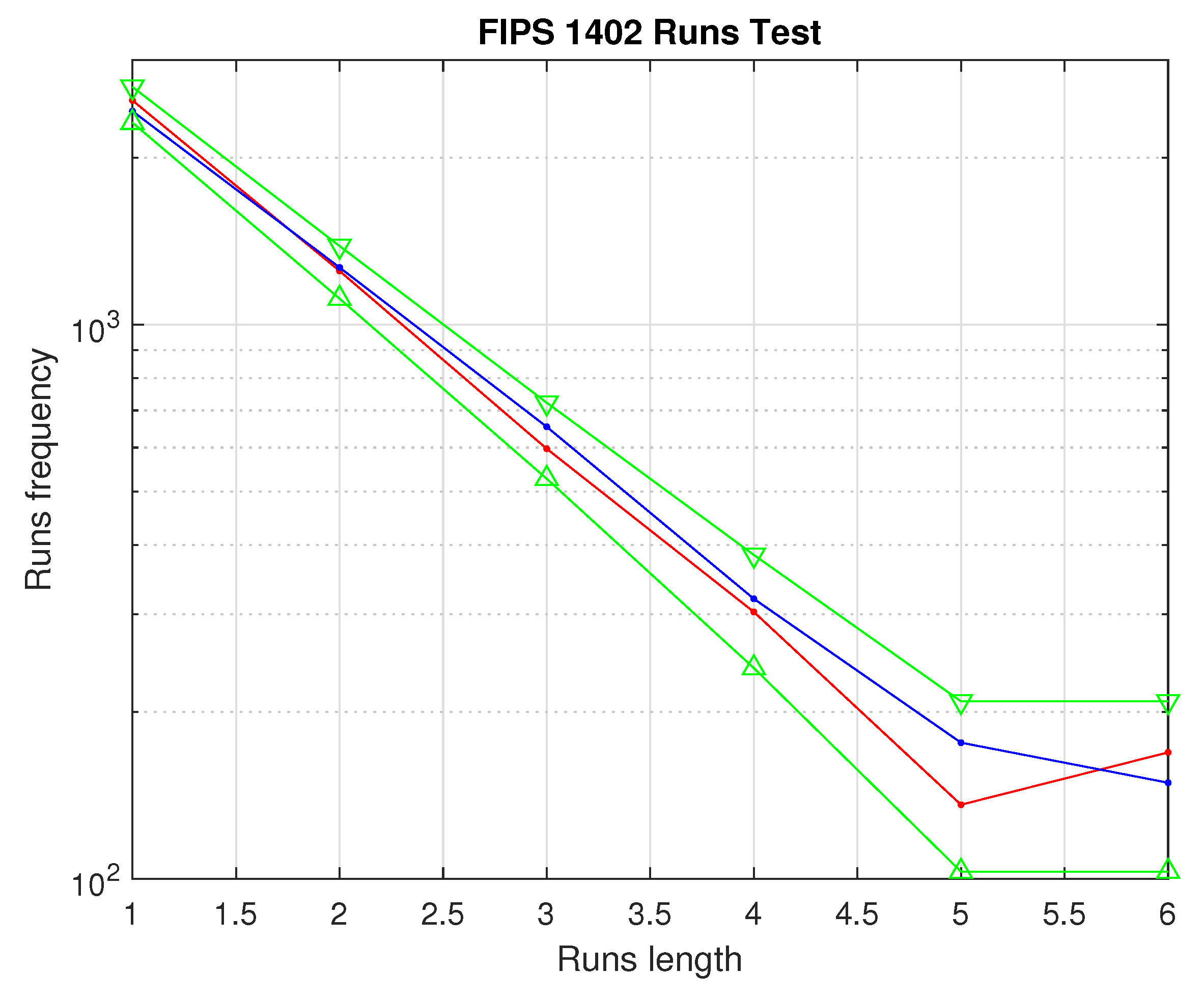
• RUNS TEST: Passed. The test is passed if the runs (for both the runs of zeros, red line, and the runs of ones, blue line) that occur (of lengths 1 through 6) are each within the corresponding interval specified in the Figure 1 by the green line.

6. Conclusions

The output sequence of the shrinking generator, the shrunken sequence, is obtained decimating the bits of a PN-sequences in terms of the bits of another PN-sequence. Besides, the shrunken sequence can be also obtained interleaving shifted versions of a unique PN-sequence. In this paper, we use the same idea of interleaving shifted versions of the same PN-sequence in order to obtain a new family of sequences with the same features as those of the shrunken sequences, that is, large period and linear complexity. We study their periods, linear complexities and the number of sequences obtained for any possible value of $LC$. Furthermore, we present a preliminary study of the randomness of t-interleaving sequences with the application of the standard FIPS, a statistical test suite for the validation of pseudorandom number generators. Through the analysis of a great number of these sequences, for different values of t and different primitive polynomials, we point out a good random behaviour.

As future work, we would like to study the open cases that we have not solved in this paper. For instance, we would like to find an analytical proof for the expressions we found on the total number of 4-interleaving sequences with $LC=3L$ and $LC=4L$; complete the study of $2^t$-interleaving sequences; and increase our knowledge about the case of t-interleaving sequences. Furthermore, we would like to do a statistical randomness analysis of these new sequences using several statistical test batteries as the Diehard battery of tests, the packet FIPS 140-2, CRYPT-X or TestU01, among others. Until now, our research is focused on the use of a PN-sequence and shifted versions of itself. A natural step would be the study of the resultant sequences of interleaving PN-sequences of different primitive polynomials (with same or different degree).