Article

Mass-Preserving Approximation of a Chemotaxis Multi-Domain Transmission Model for Microfluidic Chips

by
Elishan Christian Braun
1,†,
Gabriella Bretti
2,*,† and
Roberto Natalini
2,†
1
Department Mathematics, University of Rome 3, 00146 Rome, Italy
2
Istituto per le Applicazioni del Calcolo “M.Picone”, 00185 Rome, Italy
*
Author to whom correspondence should be addressed.
These authors contributed equally to this work.
Mathematics 2021, 9(6), 688; https://doi.org/10.3390/math9060688
Submission received: 3 March 2021 / Revised: 16 March 2021 / Accepted: 18 March 2021 / Published: 23 March 2021

Abstract

:
The present work is inspired by the recent developments in laboratory experiments made on chips, where the culturing of multiple cell species was possible. The model is based on coupled reaction-diffusion-transport equations with chemotaxis and takes into account the interactions among cell populations and the possibility of drug administration for drug testing effects. Our effort is devoted to the development of a simulation tool that is able to reproduce the chemotactic movement and the interactions between different cell species (immune and cancer cells) living in a microfluidic chip environment. The main issues faced in this work are the introduction of mass-preserving and positivity-preserving conditions, involving the balancing of incoming and outgoing fluxes passing through interfaces between 2D and 1D domains of the chip and the development of mass-preserving and positivity preserving numerical conditions at the external boundaries and at the interfaces between 2D and 1D domains.

1. Introduction

The aim of the present work is to study both the modelling and numerical approximation of a chemotaxis-reaction-diffusion mathematical system describing the qualitative behavior of different cell species living in a confined environment. This work is inspired by laboratory experiments made on microfluidic chip [1], where some populations cohexist and interact. In recent years, there has been the development of a new approach to biological studies aimed at reconstructing organs and complex biological processes on a chip [2]. The fundamental idea is that the comprehension of the sophisticated physiology of organisms, based on the complex behavior and interaction of cell populations, tissues, and organs, needs interdisciplinary contributions from biology to mathematics.
Motivated by the laboratory setting of the experiment in microfluidic chips [1,2,3]—see also the short description of the experiments reported in Section 2.1.1—we introduce a model mimicking the interactions between two cell populations—namely, immune and cancer cells.
The mathematical model, proposed in Section 2.2, is a reaction-diffusion system with chemotaxis and describes birth and death processes, the migration of immune cells driven by chemical signals produced by tumor cells, and interactions between different cell species. We underline that, since the chemical gradients are not measured experimentally, by using the simulation algorithm based on the mathematical model proposed here, the chemical concentration gradients in the chip can be obtained by solving the inverse problem of minimizing the residuals between the measured trajectories and the simulated ones; see also the discussion in Section 5 about the future developments of our work. From a mathematical point of view, we follow the framework of the classical macroscopic models of chemotaxis; see, for instance, [4], where the evolution of the density of cells is described by a parabolic equation and the concentration of a chemoattractant can be given by a parabolic or elliptic equation, depending on the different regimes to be described and on the authors’ choices. The choice of a continuous model to reproduce an experiment in a confined environment, with a relatively small number of cells, is motivated by the fact that we aim at developing a simulation tool which is able to describe the phenomena of immunosorveillance of cancer in tissues, where billions of cells are present. For this reason, a macroscopic model is more suitable respect a particle model.
In the chambers, we consider a 2D doubly parabolic model which is a modification of the Keller–Segel model [4] to take into account the presence of two populations both producing chemical signal which are interacting each other. We remark that we consider only the 2D case, since the experimental data do not take into account the height of the chip. Clearly, in principle, our framework (model and numerical algorithm) could be easily extended to the third dimension and we remark that, analogously to the 2D-1D case here considered, mass-preserving and positivity preserving numerical conditions at the external boundaries and at the interfaces between 3D and channels still hold.
We consider the microchannels connecting the 2D chambers as 1D lines for modelling and computational reasons, as explained in Section 1.1. In order to model the dynamics on the microchannels, we choose two different approaches: we can assign a 1D version of the doubly parabolic model used in the chambers; otherwise, we can assign a model derived from a 1D-GA model [5], being characterized by the more realistic feature that the speed of propagation of cells in the channels is finite, which seems the dominant property at this scale. On the other hand, other models based on hyperbolic/kinetic equations for the evolution of the density of individuals can be assigned, characterized by a finite speed of propagation [6,7,8,9,10].

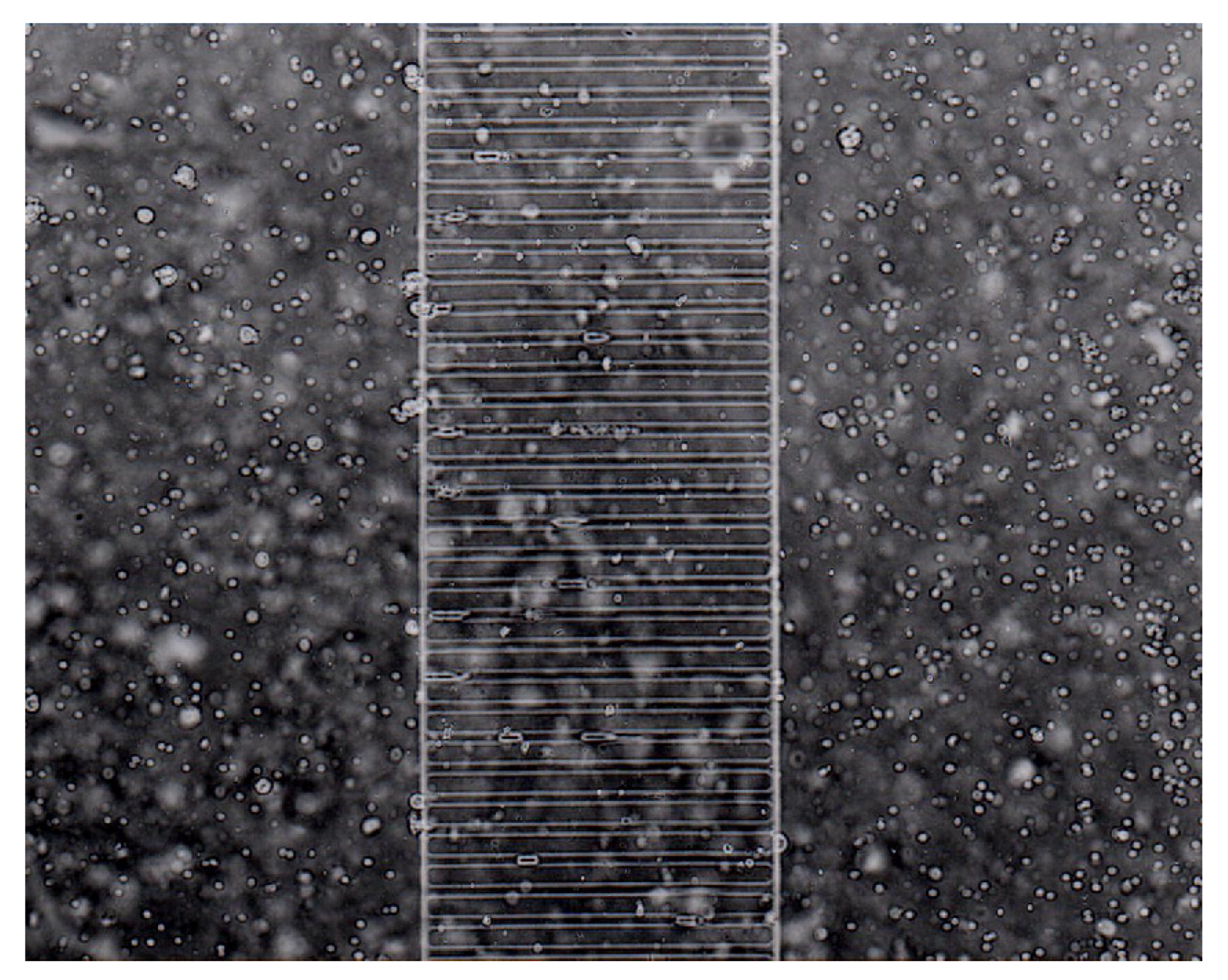
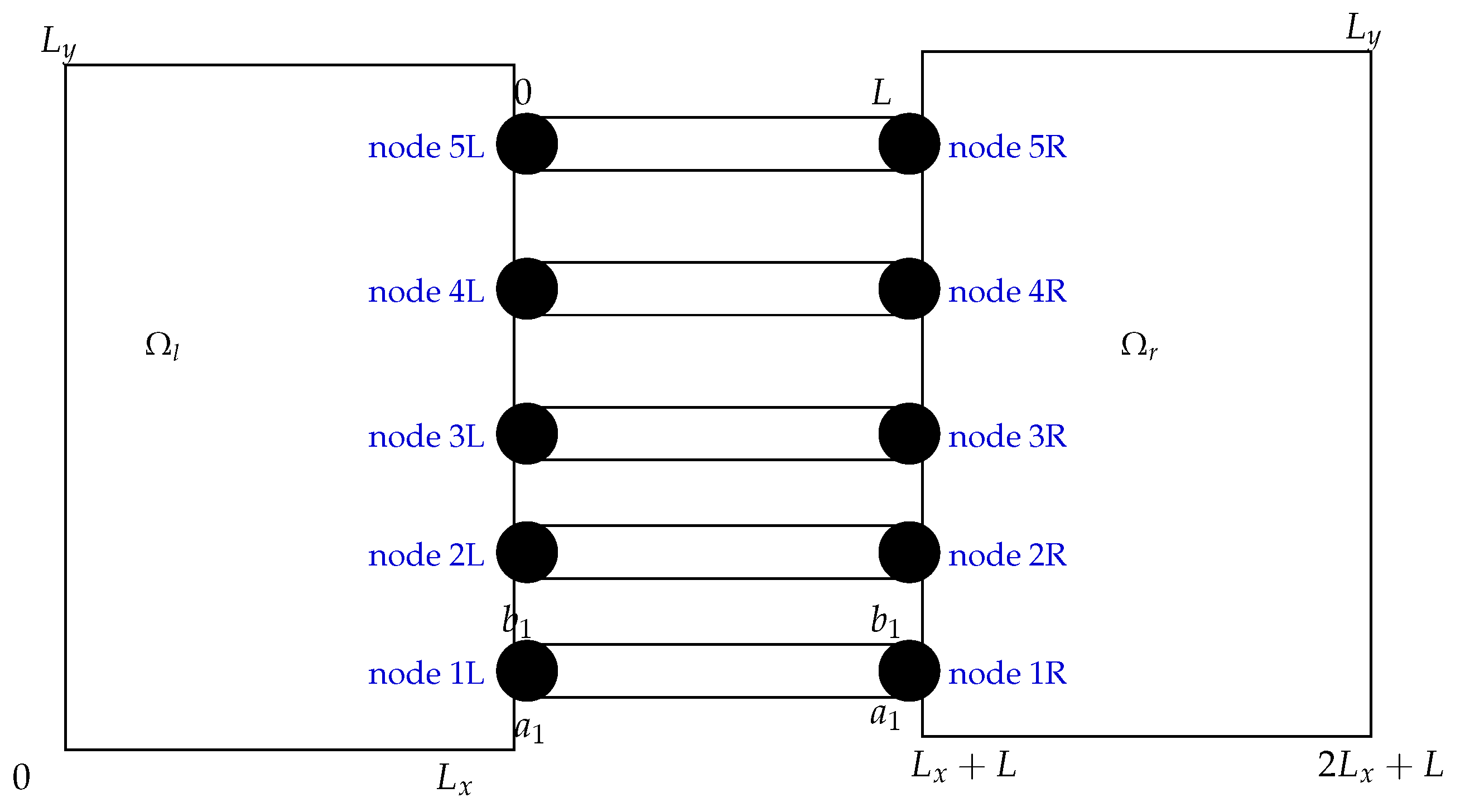
1.1. The Geometry of the Microfluidic Chip and of the Related Computational Domain

The microfluidic chip is represented as a network of channels connecting two boxes (the microfluidic chambers); see Figure 1 and a schematic picture of the related computational domain is depicted in Figure 2. Here, we refer to the experiment of two main culture chambers (a tumor and an immune cell compartment) connected via narrow capillary migration micro-channels with, respectively, width and length of 12 μ m and 500 μ m. Moreover, the channels height is of 10 μ m; however, since in the video footage the experiments is recorded at a fixed height, the third spatial dimension in our framework is neglected. The cross-sectional dimensions of culture chambers are 1 mm (width) × 100 μ m (height).
A simplified schematization of the bounded surface where the experiment is performed is reported in Figure 2. We have two microfluidic chambers of the same size, one on the left and the other on the right, defined, respectively, as Ω l = [ 0 , L x ] × [ 0 , L y ] and Ω r : = [ L x + L , 2 L x + L ] × [ 0 , L y ] . They are connected by microchannels, each of them schematized as rectangles R = [ 0 , L ] × [ a , b ] . In order to ease the reading, we point out that in the sequel we approximate the rectangular microchannels as 1D intervals C = [ 0 , L ] with zero thickness for the following reasons:
- 
modelling reason the width of microchannels (12 μ m) is comparable to the size of cells (for instance, immune cells measure about 8–10 μ m of diameter);
- 
computational reason to reduce the running time of the simulation algorithm, since otherwise we should consider a 2D meshgrid for each microchannel.
Then, the link between the box on the left and the corridor is schematized as a junction (node 1 L ) and analogously the link between the corridor and the box on the right as node 2 L . The two junctions are not really a single point, therefore they are parametrized as an interval for node 1 L and node 2 L —namely, [ a , b ] of length σ : = b a .
We remark that for the sake of simplicity, the numerical treatment is developed for a simpler geometry composed by 2D chambers connected through a single 1D channel. The extension to multiple 1D channels is done in Section 3.2.2.

1.2. Original Contribution of the Present Paper

From the mathematical and numerical viewpoint, here we deal with a challenging issue arising in the chemotaxis modelling of cell interaction. The problem involves doubly parabolic models in 2D domains (microfluifidic chambers) that are connected with 1D domains represented by channels, where either a doubly parabolic or a hyperbolic-parabolic model can be assigned.
The classical doubly parabolic Keller–Segel (KS) model [4] of chemotaxis reads as:
u t = d i v ν u χ ( ϕ ) u ϕ ϕ t = D Δ ϕ + a u b ϕ ,
with u the density of individuals in the considered medium, ν the diffusion rate of the organism according to Fick’s Law, and ϕ the density of the chemoattractant. The positive constant D is the diffusion coefficient of the chemoattractant; the positive coefficients a and b are, respectively, its production and degradation rates; and χ is the chemotactic sensitivity, depending on the density of the considered quantities. In the 2D domains given by the microfluidic chambers, we apply a reaction-diffusion chemotaxis KS-like model inspired by (1) and described in Section 2.2.1.
In the 1D microfluidic channels, we use the one-dimensional version of the KS-like model used in the chambers, but we also study the behavior of individuals when a hyperbolic-parabolic model, characterized by finite speed of propagation, is assigned. Such a hyperbolic-parabolic model, described in Section 2.2.1, is inspired by the Greeberg–Alt (GA) model, arising as a simple model for chemotaxis on a line:
t u + x v = 0 , t v + λ 2 x u = v + χ ( ϕ ) u x ϕ , t ϕ = D x x ϕ + a u b ϕ .
Note that here v is the averaged flux. Let us underline that the flux v in model (2) corresponds to v = λ 2 u + χ ( ϕ ) u ϕ for the KS system.
We remark that here we do not consider the GA model on the 2D domain, since in this case the derivation of the monotonicity condition, easily computed in 1D, it is not straightforward, due to the oscillations brought by 2D wave equation. One possibility to overcome this problem should be to consider the macroscopic hyperbolic model proposed by Preziosi in [9,11]. Alternatively, a kinetic 2D model of chemotaxis and its numerical approximation is studied in [12].
This system was analytically studied on the whole line and on bounded intervals in [13], while an effective numerical approximation, the Asymptotic High Order (AHO) scheme, was introduced in [14]—see also [15,16]—and extended on networks with general boundary conditions in [17,18].
Here, in the numerical treatment for the computation of numerical solutions one has to take care of what happens at the interface when switching from 2D-doubly parabolic models to 1D-doubly parabolic or 1D-hyperbolic-parabolic ones and vice versa.
Since we aim at reproducing the numerical solutions of such models, we need to deal with a multi-domain problem given by the passage from a 2D domain represented by the chambers of the chip to 1D domains given by the channels. For this reason we need to develop ad hoc transmission conditions to ensure mass conservation at the 2D-1D interfaces. From the numerical viewpoint, here we consider numerical boundary conditions including in the stencil a ghost cell value taken from the neighbouring domain, as we will show in the numerical Section 3. The approximation of doubly parabolic chemotaxis models for the 1D-KS model (1) on networks was already considered in [19]. However, in that case the transmission conditions were between 1D–1D interfaces and on each arc of the network the same fully parabolic model was considered. We also underline that in such work, transmission conditions required to impose the continuity of the density of both cells u and chemoattractant ϕ , while we only impose the continuity of the fluxes, which seems to be more realistic when dealing with flux of individuals or molecules.
For the numerical approximation of the GA system (2), we refer to our previous papers [14] for a single line. In particular, the numerical treatment of the hyperbolic part of the system is based on the finite difference AHO scheme with the development of mass-preserving numerical scheme at outer boundaries, while the parabolic part is approximated by finite difference and Crank–Nicolson scheme.
In [17,18] the GA system was solved on networks, thus making it necessary to develop mass-preserving transmission conditions at inner nodes (interfaces) and suitable boundary conditions at outer nodes. However, rgw transmission conditions considered there involved the mass exchange only between 1D–1D interfaces; moreover, on each arc of the network, the same model was considered. Furthermore, the second-order numerical approximation of the boundary conditions developed in such papers did not ensure the posivity preserving property in the case of oscillating functions.
The numerical approximation of permeability Kedem–Katchalsky [20] conditions describing the conservation of the flux through a node was already considered in [21], but we underline that in the mentioned paper the study was done for the approximation with finite elements methods of linear problems. For reaction-diffusion problems the approximation of permeability conditions was studied in [22] for finite difference schemes and in [23] for discontinuous Galerkin methods. The numerical treatment of permeability conditions for chemotaxis problems was presented for the first time in [24] for the 1D parabolic–parabolic interface, and a finite difference approximation was developed without taking into consideration the mass preservation nor the positivity-preservation properties at the interfaces.
Therefore, to the best of our knowledge the present paper is the first numerical work where this new technique of switching the size of the domains and type of equations (parabolic vs. hyperbolic approach) is introduced, in order to develop mass-preserving and positivity preserving schemes. We point out that in the present paper the approximation method—based on finite difference schemes—involves the derivation of suitable zero-flux boundary conditions. The motivation for our framework based on finite difference methods seems to be a natural choice when dealing with hyperbolic models of transmission.

1.3. Main Contents and Plan of the Paper

In the present paper, a positivity-preserving and mass-preserving numerical discretization of Neumann boundary conditions at the corners and at the bottom and top boundaries of the 2D domain for a 2D-doubly parabolic reaction-diffusion problem are presented. Moreover, a positivity-preserving and mass-preserving numerical scheme at the interfaces of the network connecting the 2D chambers with the 1D channels (where the 1D-doubly parabolic or 1D-hyperbolic-parabolic problem can be assigned) is developed. To summarize the main contents of the present work, the mathematical issues faced in this study are categorized into two aspects:
  • the study of the behavior of two different modelling of the dynamics in the channels: the parabolic model describing the dynamics inside the chambers was coupled both with KS-like and GA-like models;
  • the numerical approximation of equations defined in a heterogeneous domain, characterized by the switch from 2D domains, represented by microfluidic left and right chambers, to 1D domains, given by the channels connecting them.
Then, the numerical questions arising in the mentioned issues and here addressed are:
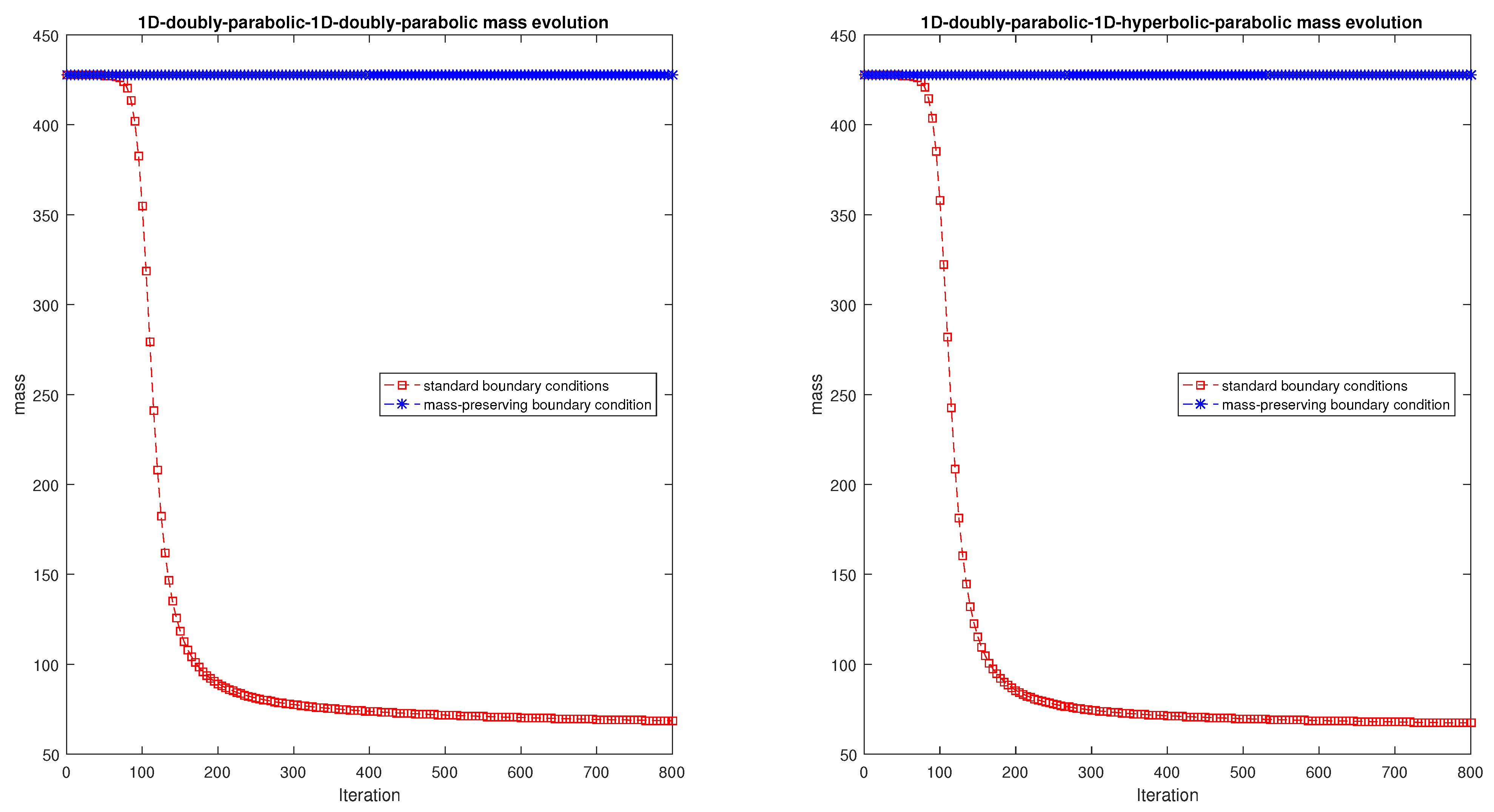
  • the study of positivity and mass-preserving external boundary conditions for 2D-doubly parabolic model (3);
  • the introduction of mass-preserving and positivity-preserving permeability conditions at the interfaces between 2D and 1D parabolic models—see Section 2.3.2;
  • the introduction of mass-preserving and positivity-preserving permeability conditions at the interfaces between the 2D-fully parabolic model and 1D-hyperbolic-parabolic model—see Section 2.3.3.
The plan of the paper is as follows. In Section 2 we describe the biological framework that inspired our study and we introduce the mathematical formulation of biologically inspired models and we introduce the adopted model. Section 3 is devoted to the numerical techniques used to approximate the problem and in Section 4 some numerical tests showing the qualitative behavior of cells in the designed environment are presented. Finally, in Section 5 a discussion on the results and the future developments of our work is presented.

2. Materials and Methods

The present Section is devoted to:
  • the description of the biological framework and the laboratory experiment that inspired our work—see Section 2.1;
  • the mathematical methods—see Section 2.2—bringing us to the development of a simulation algorithm designed for qualitatively reproducing the experimental observations.

2.1. Biological Framework

The control of immune cells migration and interaction with tumor cells living inside the chambers of the microfluidic chip, represent a new and attractive approach for the clinical management of tumor diseases. Furthermore, in the chip environment also drug testing can be exploited. Then, the quantitative assessment of immune cell migration ability to recognize and attack the tumor cells for each patient could provide a new potential parameter predictive of patient outcomes in the future.
Migrating cells respond to complex chemical stimuli (as a mixture of growth factors, cytokines, and chemokines), representing a source of chemoattractants. These chemoattractants, through the interaction with their receptors, allow cells to acquire a polarized morphology and to perform the action of immunosurveillance.
The development of lab-on-chip technologies has made it possible to realize a reproducible tailoring of the cellular microenvironment, thus allowing the continuous monitoring of experiments and the accurate control of experimental parameters. Recently, the development of microengineering has provided the possibility to realize culturing of multiple cell types and made it possible to observe cell-cell interactions and to transpose in vivo studies to a second generation of in vitro smart environments. The main advantages of this new technological tool are a close control over local experimental conditions and lower costs with respect to the use of animals in laboratory experiments for efficacy and toxicity testing. Some results obtained with on-chip experiments are presented in [1,2,25,26,27].
Regarding the structure of microfluidic devices, they are designed to allow chemical and physical contacts between tumor cells and non-adherent immune cells (i.e., murine splenocytes or human peripheral blood mononuclear cells). The microfluidic co-culture platforms are fabricated in polydimethylsiloxane (PDMS, Silgard 184), a biocompatible optically transparent silicone elastomer.

2.1.1. Setting of the Laboratory Experiments

Here, we shortly describe the laboratory experiments inspiring our work (see [1]) and carried out in the microfluidic chip environment; see Figure 1. Two populations, immune cells of wild type and cancer cells, are initially put into two separate chambers and can have physical and chemical contact through the microchannels. In more detail, rgw cells are loaded into the reservoirs as follows: the left chambers are filled with about 2 × 10 6 human peripheral blood mononuclear cells and the right chambers with about 5 × 10 4 breast cancer cells, pre-treated or not with doxorubicin hydrochloride, all immersed in a suitable culture medium. Time-lapse recordings are performed over a period of 72 h (1 microphotograph every 2 min) by means of a microscope placed directly inside the CO 2 incubator for the duration of the recording.
We consider two different scenarios:
  • first scenario (treated case): before enabling cells to migrate, tumor cells are previously treated with a chemoterapy drug. Afterwards, we observe immune cells migrating towards the left chamber where the tumor remains confined, but expresses the chemical stimuli attracting immune cells. Mainly, the dynamics observed in this case is the migration of immune cells from the right to the left in order to attack the tumor cells.
  • second scenario (untreated case): tumor cells migrate in the right chamber and proliferate. In this case, the tumor cells do not produce chemoattractant, thus immune cells move in the environment without recognizing and attacking tumor cells.
The culture medium in both cases is neutral, thus meaning that no exogenous substances are introduced. Our aim is then to build a simulation algorithm based on the mathematical model, which is able to reproduce the main features of the observed phenomena in the two scenarios.

2.2. Mathematical Framework

For the development of the mathematical modelling explained in the next section, we remark that we neglect the third dimension, since we do not have laboratory measurements of the movement of cells in the vertical direction. For this reason we consider the microfluidic chambers as 2D objects. Nowadays, the mathematical analysis of biological phenomena has become an important tool to explore complex processes and to detect mechanisms that might not be evident to the experimenters. Although a mathematical model cannot replace a real experiment, it may represent a support tool to explain acquired biological data and it may allow to gain a deeper understanding of the interactions between cancer cells and the immune system. More generally, mathematical models can describe a broad variety of biological phenomena, including cell dynamics and cancer [28,29,30,31,32].
The movement of bacteria under the effect of a chemical substance has been widely studied in the last few decades, and numerous mathematical models have been proposed. As shown in [33], chemotaxis is decisive in biological processes. For instance, the formation of cells aggregations (amoebae, bacteria, etc) occurs during the response of the different species to the change of the chemical gradients in the environment. Moreover it is possible to describe this biological phenomenon at different scales: particles models, hybrid (multiscale) models and macroscopic models.
In the present paper, the population density is assumed to be as a whole, thus macroscopic models of partial differential equations are considered. In particular, in order to describe the dynamics of cells in the 2D chambers we use a KS-like model, while in the microchannels we compare the behavior between two different modelization: a 1D KS-like model and a 1D GA-like model. The modelling here applied is described in the next Section 2.2.1.

2.2.1. The Model

Here, we introduce a mathematical model that aims at describing the behavior of two populations of cells coexisting together: tumoral cells T and immune cells (macrophages) M. We underline that the setting here considered can be made more complex with the introduction of a greater number of cell species and with the presence of an exogenous substance in the environment.
The model consists of a reaction-diffusion system with chemotaxis that it is able to describe birth and death processes, interactions with chemoattractants, interactions and competition between different cell species. The microfluidic chip is schematized as a network of channels connecting two boxes (the microfluidic chambers), then, following the ideas in [17], ad hoc transmission conditions were introduced to ensure mass conservation. The parameters of the model, such as the velocity of different cell populations, the turning rates, and the decay rates, will be calibrated with rgw observed data.
Cancer cells T produce chemical signals, called φ , activating the immune response of M and influencing their behavior. Moreover, we take into account the presence of cytokines ω (produced by M), acting as a chemical killer of cancer cells. Mainly referring to the KS model, the model here considered in the 2D chambers reads as:
t T = D T Δ T λ T ( ω ) T , t M = D M Δ M d i v ( χ ( φ ) M φ ) , t φ = D φ Δ φ + α ϕ T β φ φ , t ω = D ω Δ ω + α ω M β ω ω .
The system above describes the dynamics of the two cell species and the diffusion of the chemoattractant, and it needs to be complemented with suitable initial conditions and boundary conditions for the cells and the chemoattractant concentrations, as will be specified in the following paragraphs.
In particular, bearing in mind the first scenario (treated tumor), the system above describes the following situation: tumor cells T produce a chemical substance φ attracting immune cells M, that start migrating towards them. In this case, the tumor does not proliferate, since it is treated by a chemotherapy medicine, thus we do not include this feature in the model. Immune cells do not seem to proliferate during the experiment, thus we neglect this feature in the model. Note that, although here we are neglecting the proliferation of tumor, a tumor growth is observed experimentally in the second scenario (untreated tumor). This feature can be easily added to the model by putting a linear or logistic source term in the equation for the tumor.
Immune cells also produce a chemical substance ω which should be responsible for tumor killing. Therefore, in the first equation of the system (3), besides the diffusion term we can find λ T ( ω ) T , representing the tumor suppression operated by immune cells. We underline that at the moment we have no information from the biologists about the real killing rate in the microchip environment induced by ω , but we decided to introduce it in order to include this phenomenon in the model qualitatively.
In the second equation, in addition to the diffusion term we have the chemotactic term f = χ ( φ ) φ due to the presence of the chemical substance φ produced by the tumor.
In order to define the action of the cytotoxin ω produced by immune cells (which determines the death of cancer cells), we introduce the function λ T ( ω ) :
λ T ( ω ) = S ω γ + ω ,
where S is the maximum secretion rate of the cytotoxin by the immune cells and γ the equivalent Michaelis constant associated with the production, as described in [33]. A lot of effort has been devoted to finding a biologically accurate expression for the chemotaxis function χ ( φ ) representing the chemotactic sensitivity of immune cells; here, we refer the form suggested in [34] by Lapidis and Schiller:
χ ( φ ) = k 1 ( k 2 + φ ) 2 ,
where k 1 represents the cellular drift velocity, while k 2 is the receptor dissociation constant, which says how many molecules are necessary to bind the receptors. Note that we mainly refer to [33] for the values of the parameters k 1 , k 2 , and all the parameters of the model are reported in Table 1.
Now, in order to describe the dynamics of cells in the microchannels connecting the two boxes, we introduce the following 1D models for the dynamics, with the label c indicating the channels. Then, we consider two possible models in the channels: a diffusive one:
t T c = D T x x T c λ T ( ω ) T c , t M c = D M x x M c x ( M c f c ) , t φ c = D φ x x φ c + α φ T c β φ φ c , t ω c = D ω x x ω c + α ω M c β ω ω c ,
and a hyperbolic one:
t T c + x v c T = λ T ( ω ) T c , t v c T + D T x T c = v c T , t ω c = D ω x x ω c + α ω T c β c ω c , x M c + t v c M = 0 , t v c M + D M x M c = M c f c v c M , t φ c = D φ x x φ c + α φ T c β φ φ c ,
with T c and M c , respectively, as the density of tumor and immune cells; f c = χ ( φ c ) x φ c and v c T and v c M , respectively, as the average flux of tumor cells T c and immune cells M c in the channels. Note that the 1D-doubly parabolic model (6) is the one-dimensional version of the system (3), while (7) is the 1D-hyperbolic-parabolic model inspired by GA model [5]. We remark that, for the hyperbolic-parabolic system (7), we also need to assign initial and boundary conditions for the flux v.

2.2.2. The Simplified Model

To present the numerical scheme, we write a simpler model with respect to (3) but share the main features of it:
t u = D u Δ u div F + g ( x , y , t , u ) , t ϕ = D ϕ Δ ϕ + a u b ϕ ,
with u as the density of individuals, ϕ as the density of chemoattractant, and with F = u f . From now on, the two components of the drift term f = χ ( ϕ ) ϕ will be indicated as:
f x , y , t : = f x x , y , t f y x , y , t .
For the mono-dimensional channel, in order to make the explanation of the numerical approximation easier, we consider simpler models sharing the same characteristics of the models in (6) and (7), which read as:
t u c = D u c x x u x F c + g ( x , t , u ) , t ϕ c = D ϕ c x x ϕ c + a c u c b c ϕ c
or
t u c + x v c = g ( x , t , u c ) , t v c + λ c 2 x u c = F c v c , t ϕ c = D ϕ c x x ϕ c + a c u c b c ϕ c ,
with F c = u c f c . The systems above have to be complemented with smooth initial conditions for the unknowns u , ϕ and also v for system (10); initial data will be specified in Section 3.3. On the boundary, we consider for all the quantities homogeneous Neumann conditions, so we assume no-flux boundary conditions.
Monotonicity conditions. We also mention at this point that model (10) requires an analytical monotonicity criteria; see [35]. For a linear convection term A u c and a linear source term g = B u c , the sub-characteristic criteria
A λ c B 1 ,
must be satisfied in order for the quantity u c to be non-negative. Otherwise, having a negative u c would lead to unphysical solutions.
With regard to our former model (7), that would mean we have for the immune cell density M the monotonicity condition:
k 1 k 2 + φ c 2 | x φ c | D M .
This needs to be verified in the computational domain in order to ensure non-negative solutions.
Remark 1.
We remark that the no-flux conditions boundary conditions used in our simulations are needed to have the mass-conservation of all the quantities. However, they are not realistic, since in the laboratory experiment there is an inflow of cells from the outer boundaries. Then, we aim at extending the no-flux boundary conditions to more general ones.
In the following section, in order to discuss mass-conservation we restrict our study on a 2D closed rectangular domain named Ω n c (i.e., box without the channels) and on single lines not connected at the outer boundaries, as indicated by C n c .

2.3. Outer Boundary and Interface Conditions for the Models with Null Source Term G

From now on, we consider a further simplified version of the models presented above putting the source term g equal to zero to discuss mass conservation.

2.3.1. Boundary Conditions for the 2d Doubly Parabolic Model (8) with G = 0 .

Here, we consider the mass conservation of cell density u for zero-flux conditions at the outer boundaries of a rectangular closed domain Ω n c for the 2D model (8) with a null source term.
Indeed, since our model describes the migration of cells by both diffusion and chemoattractant effects, physically speaking the mass of cells must be preserved in the absence of the creation and destruction of cells.
For this reason, we assume a no-flux condition for the density u and the chemoattractant ϕ . Since we define the source term f as a product function of ϕ , we get the no-flux conditions:
F x , y , t n | Ω n c = 0 , u x , y , t n | δ Ω n c = 0 , ( x , y ) Ω n c ,
These guarantee mass conservation.

2.3.2. Interface between 2D-1D Models in (8) and (9)

We remark that, for simplicity, the following description focuses on the left part of the domain—i.e., Ω l and its connection with a single microchannel represented by the interval [ 0 , L ] . However, the numerical treatment holds analogously on the right side of the domain and also to multiple channels.
In the 2D left box Ω l , the position of node 1 L is at x = L y , y [ a , b ] and for the 1D domain, represented by a given number of channels C, node 1 L is placed at x = 0 (left endpoint of the channel); see Figure 2.
In order to ensure the conservation of the total mass when the mass-exchange occurs, we introduce suitable transmission conditions at the interface between 2D and 1D domains. Then, we consider the simplified models (9) or (10) for 1D channels, with g = 0 .
In particular, we have to prescribe the flux conservation at the 2D-1D interfaces, since we cannot lose or gain any cells during the passage through a node.
The conservation condition for u reads as:
d d t Ω l u x , y , t d Ω l + d d t 0 L u c x , t d x = 0 ,
and it rewrites as:
0 = Ω l D u u x , y , t F x , y , t n d S + ( D u c x u c F c ( x , t ) ) | L 0
by using the divergence theorem in the first integral. With our analytical boundary conditions, the integral vanishes, except at the boundary where the node is positioned.
We remark that attention has to be paid to n being the outer normal of the domain.
Thanks to the boundary conditions (12), we get the condition:
a b D u x u L x , y , t u ( L x , y , t ) f x ( L x , y , t ) d y = D u c x u c 0 , t F c 0 , t .
Note that in this case, the evaluation of the integrand at the right endpoint L is discarded, since we are only considering the junction connecting Ω l with the left endpoint x = 0 of the microchannel (see Figure 2).
Now, we impose Kedem–Katchalsky (KK) [20] conditions describing the conservation of the flux through a node (see also [21] for the numerical treatment of these conditions). In particular, at the interface between the left chamber and the channels, we have (on the left of node 1 L in Figure 2):
D u x u L x , y , t u L x , y , t f x L x , y , t = K u c 0 , t u ( L x , y , t ) for y a , b
On the right of node 1 L , we have:
D u c x u c 0 , t F c 0 , t = K u c ( 0 , t ) ( b a ) a b u ( L x , y , t ) d y .
Thanks to conditions (14) and (15), we are guaranteed to have the flux conservation (13), and we will use such conditions to obtain numerical boundary conditions for the boundary values at the nodes on both sides, as shown in Section 3 and in Section 3.1.2.

2.3.3. Interface between 2D-1D Models in (8)–(10)

In this section, we describe the combination of 2D parabolic-1D hyperbolic model in order to describe the dynamics with a hyperbolic model in the channels. Further care has to be given in order to keep some important properties which ensure the consistency and non-negativity of numerical solutions when connecting both models.
Now, the transmission conditions for the switch from Ω l to C = [ 0 , L ] are derived in this case. For the mass conservation of u, we impose the condition:
0 = d d t Ω l u x , y , t d Ω l + d d t 0 L u c x , t d x = Ω l D u u x , y , t div F x , y , t d Ω l + 0 L x v x , t d x Ω l D u u x , y , t F ( x , y , t ) n d S + v 0 , t = 0 .
Note that in the above formula, we have v L , t = 0 because we are looking at left interface (node 1 L ). Then, we finally get:
a 1 b 1 D u x u L x , y , t u L x , y , t ) f x ( L x , y , t d y = v 0 , t .
Now, we impose the KK-condition at the interface:
D u x u L x , y , t u ( L x , y , t ) f x L x , y , t = K u c 0 , t u L x , y , t for y a , b
Then, (16) reads as:
v 0 , t = K ( b a ) u c 0 , t + K a b u L x , y , t d y .

3. Numerical Approximation

In this section, we describe the numerical approximation of the adopted models: 2D-doubly parabolic, 1D-doubly parabolicm and 1D-hyperbolic-parabolic. We define equispaced x i : = i x , y j : = j y , and t n : = n t with x , y , t > 0 , and i = 0 , , N x + 1 , j = 0 , , N y + 1 ; for channel [ 0 , L ] , we discretize it as x i = i x , with i = 0 , , N . For a more structured presentation, we introduce the operators:
δ x 2 u i , j n : = u i + 1 , j n 2 u i , j n + u i 1 , j n , δ y 2 u i , j n : = u i , j + 1 n 2 u i , j n + u i , j 1 n , δ x 0 u i , j n : = u i + 1 , j n u i 1 , j n , δ y 0 u i , j n : = u i , j + 1 n u i , j 1 n , δ x 1 u i , j n : = u i + 1 , j n u i , j n , δ y 1 u i , j n : = u i , j + 1 n u i , j n .
Remark 2.
Note that special attention has to be paid also to the stiffness induced by the source term g x , y , t , u . To overcome this issue, implicit methods can be used, such as the Crank–Nicolson method, which is associated with a Δ t that is small enough.
Mass-preserving and (numerically)-positivity-preserving approximations will be developed in the present section. In the following, we will neglect the label c to make the reading easier and we will make distinctions only when necessary.

3.1. The Parabolic-Parabolic Case

Here, we introduce a numerical scheme for the doubly parabolic systems (8) and (9) for g = 0 .
For the discretization of equations in a 2D system (8) in the interior points of the domain—i.e., for i = 1 , , N x , j = 1 , , N y , we define a finite difference discretization both for u and ϕ :
u i , j n + 1 = u i , j n + D u t 2 δ x 2 ( u i , j n + u i , j n + 1 ) x 2 + δ y 2 ( u i , j n + u i , j n + 1 ) y 2 t ( δ x 0 F i , j x , n + δ y 0 F i , j y , n ) ,
ϕ i , j n + 1 = ϕ i , j n + D ϕ t 2 δ x 2 ϕ i , j n + ϕ i , j n + 1 x 2 + δ y 2 ϕ i , j n + ϕ i , j n + 1 y 2 + t 2 a ( u i , j n + u i , j n + 1 ) t 2 b ( ϕ i , j n + ϕ i , j n + 1 ) .
Note that F i x , n = χ ( ϕ i , j n ) u i , j n δ x 0 ϕ i , j n with δ x 0 ϕ i , j n a centered second order approximation of ϕ x .
For a 1D system (9), in the interior points of the channel C we apply the Crank–Nicolson scheme, as above:
u i c , n + 1 = u i c , n + D u c Δ t 2 δ x 2 u i c , n + u i c , n + 1 x 2 Δ t δ x 0 F c , i n ,
ϕ i c , n + 1 = ϕ i c , n + D ϕ c t 2 δ x 2 ϕ i c , n + ϕ i c , n + 1 x 2 + t 2 a c ( u i c , n + u i c , n + 1 ) t 2 b c ( ϕ i c , n + ϕ i c , n + 1 ) .
Remark 3.
We remark that here, for simplicity, upwinding terms needed to avoid meshgrid restrictions caused by a large Péclet number—see, for instance [36]—are not included in the schemes (18) and (20). In this case, assuming a small Δ x and Δ y will be enough to avoid oscillations.
The upwinding be added in the implemented scheme described in Section 3.3.
Stability condition. By using the Von-Neumann stability analysis on the linearized problem, we derive the following condition for the Crank–Nicolson schemes above, [37]:
D u t x 2 1 for 1 D , D u t x 2 + D u t y 2 1 for 2 D .
In the following, we present the discretization of the boundary and transmission conditions to complete the numerical schemes.

3.1.1. Discretization of the Outer Boundary Conditions for the Doubly Parabolic Problem

Since a qualitative characteristic of the model is the preservation of total mass for zero-flux boundary conditions, the first step is to ensure the mass preservation at each time step in a closed 1D line C n c and, analogously, in a closed 2D chamber, namely Ω n c . To this aim, we have to choose discrete boundary conditions that both are consistent with the analytical boundary conditions and preserve the mass in the numerical method. We remark that we present the computations without source term g, and we will add it in the following to complete the equations.
Boundary conditions for the density of individuals u in 1D model (9).
Here, we consider Neumann boundary conditions u x ( x , t ) = 0 . If we discretized it with a (standard) forward finite difference scheme:
x u ( 0 ) = u 1 c , n u 0 c , n Δ x ,
the mass will not be preserved over time, as shown in the numerical Example 1. Therefore, in order to have mass preservation, we use the central finite difference approximation with a ghost cell:
x u ( 0 ) = u 1 c , n u 1 c , n 2 Δ x .
At the outer boundaries at the first ( x 0 = 0 ) and last ( x N + 1 = L ) endpoint of the channels, we assign the numerical schemes:
u 0 c , n + 1 = u 0 c , n + D u c t x 2 δ x 1 u 0 c , n + u 0 c , n + 1 t x ( F c , 1 n + F c , 0 n )
and
u N + 1 c , n + 1 = u N + 1 c , n D u c t x 2 δ x 1 u N c , n + u N c , n + 1 + t x ( F c , N n + F c , N + 1 n ) ,
with F c , 0 n = 0 in (25) and F c , N + 1 n = 0 in (26), since we are imposing zero flux at the boundaries. The boundary conditions above are mass-preserving by construction, as stated in the following proposition.
Proposition 1.
The 1D numerical scheme at the internal points introduced above, namely:
u i c , n + 1 = u i c , n + D u c t 2 x 2 δ x 2 ( u i c , n + u i c , n + 1 ) t 2 x δ x 0 F c , i n ,
endowed with boundary conditions (25) and (26), is mass-preserving by construction, since it is obtained by imposing I n + 1 I n = 0 .
Proof. 
The mass conservation over time on the closed domain Ω n c reads as:
I ( t ) = Ω n c u t , x , y d Ω n c = Ω n c u 0 , x , y d Ω n c = I ( 0 ) .
Now, applying a quadrature rule for the numerical integration:
I n Ω n c u t , x , y d Ω n c .
We need to ensure that I n + 1 = I n .
For the numerical integration, different quadrature formulas can be used; in particular, we applied closed Newton–Cotes formulas to take into account the values at the boundaries. By using the trapezoidal rule with an integration error of O x 2 and imposing the equality I n + 1 I n = 0 in the 1D case, one obtains:
x u 0 c , n + 1 2 u 0 c , n 2 + i = 1 N u i c , n + 1 u i c , n + u N + 1 c , n + 1 2 u N + 1 c , n 2 = 0 .
Using the numerical scheme (20) for u i c , n + 1 in (30) for i = 1 , , N we have:
x u 0 c , n + 1 u 0 c , n 2 + D u c t 2 x 2 i = 1 N δ x 2 u i c , n + u i c , n + 1 t 2 x i = 1 N δ x 0 F c , i n + u N + 1 c , n + 1 u N + 1 c , n 2 = 0 .
Now, using the definition of δ x 0 F c , i n in the sum, the above formula becomes:
u 0 c , n + 1 u 0 c , n D u c t x 2 u 1 c , n + u 1 c , n + 1 ( u 0 c , n + u 0 c , n + 1 ) + t x F c , 0 n + F c , 1 n + u N + 1 c , n + 1 u N + 1 c , n D u c t x 2 u N c , n + u N c , n + 1 ( u N + 1 c , n + u N + 1 c , n + 1 ) t x F c , N n + F c , N + 1 n = 0 .
We can now compute the values for both u 0 n + 1 and u N + 1 n + 1 so that the term equals zero. By collecting values from nearby stencils together (otherwise we obtain an error of O ( x ) , which can be verified by Taylor expansion), at the outer boundaries of 1D domain we obtain the schemes (25) and (26). Note that in the formula above, by imposing homogeneous Neumann boundary conditions we have f 0 n = 0 and f N + 1 n = 0 .
We also remark that besides imposing the stability condition (22), Δ x has to be small enough in order to ensure the positivity of the scheme for taking into account the possibility of having a negative term brought by f 1 n or f N n in (25) and (26), respectively. □
Remark 4.
Although here we are not proving that, the scheme (27) is in practice second order in the space up to the boundaries, since it can be equivalently obtained using the second-order approximation of the first derivative including a ghost cell reported in (24).
We underline that for f 0 , even using formula (24), the approach with the discrete integral equation is necessary for ensuring the mass preservation. Furthermore, by using a different numerical integration scheme, we can achieve different mass-preserving boundary conditions of a higher order.
Boundary conditions for the density of individuals u in 2D model (8).
Let us assume there are no-flux conditions at the boundaries. Then, in this case we consider the 2D closed domain Ω n c .
Using the mass-preserving property argument, we compute boundary conditions for the corners and the top and bottom boundaries of Ω n c . By applying them with the numerical method (18) into I n + 1 I n = 0 , we obtain the expression:
t x 4 4 t i = 1 N x j = 1 N y δ x 0 F i , j x + δ y 0 F i , j y = 0 ,
since the terms in u cancel. By plugging in it the expression of the central in rgw space second-order finite difference scheme δ x 0 f j x , n for div f , we obtain:
1 y i = 1 N x F i , N y + 1 y , n + F i , N y y , n F i , 1 y , n F i , 0 y , n + 1 x j = 1 N y F N x + 1 , j x , n + F N x , j x , n F 1 , j x , n F 0 , j x , n = 0 .
Now, we can distribute the remaining values to the boundaries in the same way as above for the 1D-parabolic case. Therefore, we obtain the following mass-preserving boundary conditions for the corners:
u 0 , 0 n + 1 = u 0 , 0 n + D u t 2 x 2 δ x 1 u 0 , 0 n + u 0 , 0 n + 1 + D u t 2 y 2 δ y 1 u 0 , 0 n + u 0 , 0 n + 1 , u N x + 1 , 0 n + 1 = u N x + 1 , 0 n D u t 2 x 2 δ x 1 u N x , 0 n + u N x , 0 n + 1 + D u t 2 y 2 δ y 1 u N x + 1 , 0 n + u N x + 1 , 0 n + 1 , u 0 , N y + 1 n + 1 = u 0 , N y + 1 n + D u t 2 x 2 δ x 1 u 0 , N y + 1 n + u 0 , N y + 1 n + 1 D u t 2 y 2 δ y 1 u 0 , N y n + u 0 , N y n + 1 , u N x + 1 , N y + 1 n + 1 = u N x + 1 , N y + 1 n D u t 2 x 2 δ x 1 u N x , N y + 1 n + u N x , N y + 1 n + 1 D u t 2 y 2 δ y 1 u N x + 1 , N y n + u N x + 1 , N y n + 1 .
For the edges of the box Ω n c , i = 1 , , N x and j = 1 , , N y , we have:
u i , 0 n + 1 = u i , 0 n + D u t 2 x 2 δ x 2 u i , 0 n + u i , 0 n + 1 + D u t y 2 δ y 1 u i , 0 n + u i , 0 n + 1 t y F i , 1 y , n , u i , N y + 1 n + 1 = u i , N y + 1 n + D u t 2 x 2 δ x 2 u i , N y + 1 n + u i , N y + 1 n + 1 D u t y 2 δ y 1 u i , N y n + u i , N y n + 1 + t y F i , N y y , n , u 0 , j n + 1 = u 0 , j n + D u t x 2 δ x 1 u 0 , j n + u 0 , j n + 1 + D u t 2 y 2 δ y 2 u 0 , j n + u 0 , j n + 1 t x F 1 , j x , n , u N x + 1 , j n + 1 = u N x + 1 , j n D u t x 2 δ x 1 u N x , j n + u N x , j n + 1 + D u t 2 y 2 δ y 2 u N x + 1 , j n + u N x + 1 , j n + 1 + t x F i , N y y , n .
We underline that in the above formulas the terms F x , n and F y , n on the edges of the domain cancel because of the homogeneous Neumann boundary condition on ϕ x and ϕ y .
Boundary conditions for the density of chemoattractant ϕ in 1D model (9).
For the computation of the conditions at the outer boundaries for the chemoattractant ϕ c in the 1D-doubly parabolic model we proceed as above, but neglect the source term a c u c b c ϕ c to obtain boundary conditions that are mass-preserving.
Proceeding as above, we achieve the following mass-preserving boundary conditions for the chemoattractant:
ϕ 0 c , n + 1 = ϕ 0 c , n + D ϕ c t x 2 δ x 1 ϕ 0 c , n + δ x 1 ϕ 0 c , n + 1 ϕ N + 1 c , n + 1 = ϕ N + 1 c , n D ϕ c t x 2 δ x 1 ϕ N c , n + δ x 1 ϕ N c , n + 1
This, under the CFL condition (22), is second-order accurate and positivity-preserving up to the boundaries. The parabolic equation in the interior points is solved using an implicit-explicit method:
ϕ i c , n + 1 = ϕ i c , n + D ϕ c t 2 x 2 δ x 2 ϕ i c , n + ϕ i c , n + 1 .
Boundary conditions for the density of chemoattractant ϕ in 2D model (8).
Reasoning as above, by applying the numerical method (19) we obtain the following boundary condition for the chemoattractant at the corners:
ϕ 0 , 0 n + 1 = ϕ 0 , 0 n + D ϕ t x 2 δ x 1 ( ϕ 0 , 0 n + ϕ 0 , 0 n + 1 ) + 2 D ϕ t y 2 δ y 1 ( ϕ 0 , 0 n + ϕ 0 , 0 n + 1 ) ϕ N x + 1 , 0 n + 1 = ϕ N x + 1 , 0 n D ϕ t x 2 δ x 1 ( ϕ N x + 1 , 0 n + ϕ N x + 1 , 0 n + 1 ) + D ϕ t y 2 δ y 1 ( ϕ N x + 1 , 0 n + ϕ N x + 1 , 0 n ) ϕ N x + 1 , N y + 1 n + 1 = ϕ N x + 1 , N y + 1 n D ϕ t x 2 δ x 1 ( ϕ N x , N y + 1 n + ϕ N x , N y + 1 n + 1 ) D ϕ t y 2 δ x 1 ( ϕ N x + 1 , N y + 1 n + ϕ N x + 1 , N y n ) ϕ 0 , N y + 1 n + 1 = ϕ 0 , 0 n + D ϕ t x 2 δ x 1 ( ϕ 1 , N y + 1 n + ϕ 1 , N y + 1 n + 1 ) D ϕ t y 2 δ y 1 ( ϕ 0 , N y n + ϕ 0 , N y n + 1 )
and
ϕ i , 0 n + 1 = ϕ i , 0 n + D ϕ t x 2 δ x 2 ( ϕ i , 0 n + ϕ i , 0 n + 1 ) + 2 D ϕ t y 2 δ y 1 ( ϕ i , 0 n + ϕ i , 0 n + 1 ) ϕ i , N y + 1 n + 1 = ϕ i , N y + 1 n + D ϕ t x 2 δ x 2 ( ϕ i , N y + 1 n + ϕ i , N y + 1 n + 1 ) 2 D ϕ t y 2 δ y 1 ( ϕ i , N y n + ϕ i , N y n + 1 ) ϕ 0 , j n + 1 = ϕ 0 , j n + D ϕ t y 2 δ y 2 ( ϕ 0 , j n + ϕ 0 , j n + 1 ) + 2 D ϕ t x 2 δ x 1 ( ϕ 0 , j n + ϕ 0 , j n + 1 ) ϕ N x + 1 , j n + 1 = ϕ N x + 1 , j n + D ϕ t y 2 δ y 2 ( ϕ N x + 1 , j n + ϕ N x + 1 , j n + 1 ) . 2 D ϕ t x 2 δ x 1 ( ϕ N x , j n + ϕ N x , j n + 1 )
We now have a complete numerical method to solve the system (8) on Ω n c and the 1D version of it (9) on C n c .
Let us now turn to the complete domain depicted in Figure 2 in order to develop mass-preserving transmission conditions at the nodes of the network. We remark that for the sake of clarity, for the development of the numerical transmission conditions here we consider just the junction—indicated as node 1 L —connecting the left box Ω l and a single channel parametrized as an interval C = [ a , b ] .

3.1.2. Discretization of the Transmission Conditions for the 2D-1D Doubly Parabolic Case

The choice of suitable transmission conditions is crucial, since it should reflect the qualitative attributes of the analytical model.
Here, we use ghost values (24) in order to obtain the numerical boundary conditions, since in such a way mass-preserving and positivity-preserving properties are ensured.
By using the central approximation formula for d i v f in the condition (14) on the left of node 1 L , we have:
D u x u L x , y , t F x L x , y , t = K u c 0 , t u L x , y , t   for   y a , b .
Then we have:
D u u N x + 2 , j n u N x , j n 2 x = K u 0 c , n u N x + 1 , j n + F N x + 1 , j x , n
and we get:
u N x + 2 , j n = u N x , j n + K 2 x D u 0 c , n u N x + 1 , j n + 2 x D u F N x + 1 , j x , n
for j = j a , , j b .
Moreover, using the central approximation for x u c in (15),
we finally get the formula:
u 1 c , n = u 1 c , n K 2 x D u c ( b a ) u 0 c , n + 2 x D u c Δ y j = j a j b K ( u N x + 1 , j n + u N x + 1 , j n + 1 ) 2 x D u c F c , 0 n .
We now use the Ansatz to apply the ghost values into the 1D (27) and 2D (18) numerical schemes without specific chemotactic approximation, and use the discrete integral equation to determine the chemotactic term discretization.
Since we need to conserve the mass in each domain, but also in both connected ones, the expanded discrete integral equation is needed to compute the total mass over both domains.
Plugging the ghost values (36) and (37), respectively, into the numerical schemes (18) and (27), we get the conditions at the interface (node 1 L ):
u N x + 1 , j n + 1 = u N x + 1 , j n D u t x 2 δ x 1 u N x , j n + u N x , j n + 1 + 2 K t x u 0 c , n u N x + 1 , j n + D u t 2 y 2 δ y 2 u N x + 1 , j n + u N x + 1 , j n + 1 + 2 t x F N x + 1 , j x , n t δ x 0 F N x + 1 , j x , n t δ y 0 F N x + 1 y , n ,
and
u 0 c , n + 1 = u 0 c , n + D u c t x 2 δ x 1 u 0 c , n + u 0 c , n + 1 2 K t x ( b a ) u 0 c , n + 2 K t y x j = j a j b u N x + 1 , j n + u N x + 1 , j n + 1 2 t x F c , 0 n t 2 Δ x δ x 0 F c , 0 n .
In particular, the conservation of the discrete total mass reads as:
I 1 D n + 1 + I 2 D n + 1 I 1 D n I 2 D n = 0 ,
Now, applying the conditions (38) and (39) with the other boundary conditions (31) and (25), we get:
x ( K t x ( b a ) u 0 c , n + K t y x j = j a j b u N x + 1 , j n + u N x + 1 , j n + 1 t x F c , 0 n t 2 δ x 0 F c , 0 n + t 2 x F c , 0 n + F c , 1 n ) + x y 4 ( 2 j = j a j b ( 2 K t x u 0 c , n u N x + 1 , j n + 2 t x F N x + 1 , j x , n t δ x 0 F N x + 1 , j x , n t δ y 0 F N x + 1 , j y , n ) 2 t x j = j a 1 j b 1 F N x + 1 , j x , n + F N x , j x , n 2 t y j = j a j b F N x + 1 , j y , n + F N x , j y , n ) = 0 ,
We can then obtain the following transmission conditions:
u 0 c , n + 1 = u 0 c , n + D u c t x 2 δ x 1 u 0 c , n + u 0 c , n + 1 t x ( F c , 1 n + F c , 0 n ) same as for BC without transmission condition 2 K t x ( b a ) u 0 c , n + 2 K t x j = j a j b u N x + 1 , j n + u N x + 1 , j n + 1 ,
u N x + 1 , j n + 1 = u N x + 1 , j n D u t x 2 δ x 1 u N x , j n + u N x , j n + 1 + D u t 2 y 2 δ y 2 u N x + 1 , j n + u N x + 1 , j n + 1 + t x F N x + 1 , j x , n + F N x , j x , n t 2 y F N x + 1 , j + 1 y , n F N x + 1 , j 1 y , n + 2 K t x u 0 c , n u N x + 1 , j n additional term for transmission condition ,
for j = j a , , j b .
Proceeding analogously as above, this approach leads to mass-preserving and positivity-preserving transmission conditions for the chemoattractant ϕ as well. In particular, we have at the first and last endpoint, respectively:
ϕ 0 c , n + 1 = ϕ 0 c , n + D ϕ c t x 2 δ x 1 ϕ 0 c , n + δ x 1 ϕ 0 c , n + 1 + t a c u 0 c , n t b c ϕ 0 c , n 2 K t x ( b a ) ϕ 0 c , n + 2 K t x a b ϕ L x , y , t n d y
and
ϕ N x + 1 , j n + 1 = ϕ N x + 1 , j n + D ϕ t y 2 δ y 2 ( ϕ N x + 1 , j n + ϕ N x + 1 , j n + 1 ) 2 D ϕ t x 2 δ x 1 ( ϕ N x , j n + ϕ N x , j n + 1 ) + a t u N x + 1 , j n b t ϕ N x + 1 , j n + 2 K t x ϕ 0 c , n ϕ N x + 1 , j n .
We have finally developed a complete numerical scheme to treat doubly parabolic partial differential equations systems in two domains, 1D and 2D, connected through a node, which ensures by construction the mass conservation as the original PDE. Numerically, the scheme also ensures the positivity preserving property under the monotonicity conditions discussed in Section 3.3.1.

3.2. The Hyperbolic-Parabolic Case

The second-order AHO scheme on a line was introduced in [14] for the 1D hyperbolic system (2). Here, considering the presence of the source term g on the right hand side of the equation for the density of cells, the AHO scheme of second order reads as:
u i c , n + 1 = u i c , n + λ t 2 x δ x 2 u i c , n t 2 x t 4 λ δ x 0 v i c , n + t 4 λ δ x 0 F c , i n + t 4 g i 1 n + 2 g i n + g i + 1 n , v i c , n + 1 = v i c , n λ 2 t 2 x δ x 0 u i c , n + λ t 2 x t 4 δ x 2 v i c , n + t 4 δ x 2 F c , i n + λ t 4 g i 1 n g i + 1 n ,
with mass-preserving boundary conditions (including the additional source term g) at the external boundaries.
We remark that for the hyperbolic-parabolic model not only mass must be preserved as the in the fully parabolic model, but also the flux v needs to converge towards the steady state v = 0 . Since here we have the 1D domain connected at both the endpoints, we do not need to use numerical boundary conditions for the outer boundaries. However, for the details and the description of the AHO numerical scheme at the outer boundaries, see [14]. For this reason we use the so-called AHO (Asymptotic Higher Order) schemes (see [18] for the study of AHO scheme at interfaces including mass-preserving transmission conditions) with source term g, for which the approximation of the stationary solutions is up to the third order of accuracy and converges towards a numerical solution with v = 0 , while preserving the mass.

3.2.1. Discretization of Transmission Conditions for the 2D-Doubly Parabolic and 1D-Hyperbolic-Parabolic Case

The first equation is the same as for the interface between the 2D-doubly parabolic and 1D-doubly parabolic case. Hence, we derive the same transmission condition reported in (42) for u N x + 1 , j n + 1 for j = j a , , j b .
For the flux, the transmission condition (17) gives us
v 0 c , n + 1 = K ( b a ) u 0 c , n + 1 + K y j = j a j b u N x + 1 , j n + u N x + 1 , j n + 1 ,
This can be computed explicitly with the numerically computed values of u 0 c , n + 1 and u N x + 1 , j n + 1 .
Then, imposing the mass conservation:
I 2 D n + 1 + I 2 D n + 1 I 1 D n I 1 D n = 0
we get:
x 2 u 0 c , n + 1 u 0 c , n + λ t x u 0 c , n + 1 u 1 c , n + 1 t x t 2 λ v 0 c , n + 1 v 1 c , n + 1 + x t 4 λ F c , 0 n + 1 + F c , 1 n + 1 + x y 4 4 j = j a j b t K x u 0 c , n + 1 + u 0 c , n u N x + 1 , j n + 1 u N x + 1 , j n = 0
We thus finally obtain the mass-preserving transmission condition, where we finally add the source term g, as:
u 0 c , n + 1 = u 0 c , n + λ t x δ x 1 u 0 c , n + 1 t x t 2 λ v 0 c , n + 1 + v 1 c , n + 1 K t x y j = j a j b u 0 c , n + 1 + u 0 c , n u N x + 1 , j n + 1 u N x + 1 , j n t 2 λ F c , 0 n + 1 + F c , 1 n + 1 + t 2 g 0 n + 1 + g 1 n + 1 .
Proposition 2.
The complete numerical scheme derived for the 2D-doubly parabolic-1D-hyperbolic-parabolic model is mass-preserving—by construction—across the transmission conditions in absence of source terms.
Remark 5.
Note that the chemoattractant equation is the same as for the 1D-doubly parabolic and 2D-doubly parabolic case. Hence, the numerical schemes (33) and (19) with boundary conditions (32) and (43) can be used.

3.2.2. Multiple Channels

In the previous paragraphs, we connected the two-dimensional domain Ω l with a single one-dimensional channel C at ( L x , y ) Ω l with y a 1 , b 1 , and j a 1 and j b 1 , the positions of the endpoints of the corridor on the numerical grid. Of course, this can be extended to more channels.
Let C m , with m = 1 , , M be M corridors, connected to the two-dimensional domain Ω l at L x , y m with y m a m , b m and a 1 > 0 , b m < a m + 1 , for m = 1 , , M 1 , and b M < L y to avoid intersections of the corridors, with equal width k y , k N .

3.3. Implemented Algorithm.

Before presenting the numerical tests in the next Section 4, we adapt the approximation scheme for the density u, also including the source term g, implemented to solve the problem in the 2D-1D domain. As underlined before, it is necessary to use implicit schemes to consider the presence of stiff source terms. For this reason, for the approximation of the time derivatives we use the Crank–Nicolson (CN) method on the diffusion and source term, which is a second-order implicit method and the explicit central method for the convection term. Moreover, since CN is only A-stable but not L-stable [38], we also need to choose a Δ t that is small enough to avoid spurious oscillations of the solution during transience.
Because of the explicit term, we have numerical restrictions on the mesh grid and time step. Furthermore, as discussed previously, we introduce artificial viscosity to avoid oscillations due to not suitable mesh grid size in dominant convection regime, which is often the case in chemotaxis models. Finally, the implicit-explicit numerical method used to compute the solutions for the density u in (8) inside the 2D domain Ω l is:
u i , j n + 1 = u i , j n + D u t 2 δ x 2 ( u i , j n + u i , j n + 1 ) x 2 + δ y 2 ( u i , j n + u i , j n + 1 ) y 2 t 4 δ x 0 F i , j x , n x + δ y 0 F i , j y , n y + t 2 g i , j n + g i , j n + 1 t δ x 2 θ i , j n 2 x + δ y 2 θ i , j n 2 y artificial viscosity ,
with: θ i , j n : = χ ( φ i , k n ) u i , j n | φ i , j n | for i = 1 , , N x , j = 1 , , N y . As can be seen, the function θ used for the artificial viscosity is almost identical to f, with the exception of using the absolute value of φ . By using this, we increase artificial viscosity only where the gradient of the chemoattractant increases. This reduces the restriction on the meshgrid due to the condition induced by the cell Péclet number, [36]. The numerical transmission condition on the left of node 1 L ( i = N x + 1 , j = j a , , j b ) is:
u N x + 1 , j n + 1 = u N x + 1 , j n D u t x 2 δ x 1 ( u N x , j n + u N x , j n + 1 ) + D u t 2 y 2 δ y 2 u N x + 1 , j n + u N x + 1 , j n + 1 + t x F N x + 1 , j x , n + F N x , j x , n t y F N x + 1 , j + 1 y , n F N x + 1 , j 1 y , n + t 2 g N x + 1 , j n + g N x + 1 , j n + 1 t δ x 1 θ N x , j n x + δ y 2 θ N x + 1 , j n 2 y + K t x u 0 c , n u N x + 1 , j n + u 0 c , n + 1 u N x + 1 , j n + 1 ( additional term for transmission condition ) .
The role of permeability coefficient K in the positivity of (48) is discussed in Section 3.3.1.
For the external boundaries (the edges of the chamber Ω l except at the junctions j = j a , , j b ), we use:
u i , 0 n + 1 = u i , 0 n + D u t 2 x 2 δ x 2 u i , 0 n + u i , 0 n + 1 + D u t y 2 δ y 1 u i , 0 n + u i , 0 n + 1 t 2 x δ x 0 F i , 0 x , n t y F i , 0 y , n + F i , 1 y , n + t 2 g i , 0 n + g i , 0 n + 1 t δ x 2 θ i , 0 n 2 x + δ y 1 θ i , 0 n y , i = 1 , , N x , u i , N y + 1 n + 1 = u i , N y + 1 n + D u t 2 x 2 δ x 2 u i , N y + 1 n + u i , N y + 1 n + 1 D u t y 2 δ y 1 u i , N y n + u i , N y n + 1 t 2 x δ x 0 F i , N y + 1 x , n + t y F i , N y y , n + F i , N y + 1 y , n + t 2 g i , N y + 1 n + g i , N y + 1 n + 1 t δ x 2 θ i , N y + 1 n 2 x + δ y 1 θ i , N y n y , i = 1 , , N x , u 0 , j n + 1 = u 0 , j n + D u t x 2 δ x 1 u 0 , j n + u 0 , j n + 1 + D u t 2 y 2 δ y 2 u 0 , j n + u 0 , j n + 1 t x F 0 , j x , n + F 1 , j x , n t 2 y δ y 0 F 0 , j y , n + t 2 g 0 , j n + g 0 , j n + 1 t δ x 1 θ 0 , j n x + δ y 2 θ 0 , j n 2 y , j = 1 , , N y , u N x + 1 , j n + 1 = u N x + 1 , j n D u t x 2 δ x 1 u N x , j n + u N x , j n + 1 + D t 2 y 2 δ y 2 u N x + 1 , j n + u N x + 1 , j n + 1 t 2 x δ x 0 F i , N y + 1 x , n + t x F i , N y y , n + F i , N y + 1 y , n + t 2 g N x + 1 , j n + g N x + 1 , j n + 1 t δ x 1 θ N x , j n x + δ y 2 θ N x + 1 , j n 2 y , j = 1 , , N y , j j a , , j b .
For the corners, we use the following boundary conditions:
u 0 , 0 n + 1 = u 0 , 0 n + D u t x 2 δ x 1 u 0 , 0 n + u 0 , 0 n + 1 + D u t y 2 δ y 1 u 0 , 0 n + u 0 , 0 n + 1 t x F 0 , 0 x , n + F 1 , 0 x , n t y F 0 , 0 y , n + F 0 , 1 y , n + t 2 g 0 , 0 n + g 0 , 0 n + 1 t δ x 1 θ 0 , 0 n x + δ y 0 θ 0 , 0 n y , u N x + 1 , 0 n + 1 = u N x + 1 , 0 n D u t x 2 δ x 1 u N x , 0 n + u N x , 0 n + 1 + D u t y 2 δ y 1 u N x + 1 , 0 n + u N x + 1 , 0 n + 1 t x F N x + 1 , 0 x , n + F N x , 0 x , n t y F N x + 1 , 0 y , n + F N x + 1 , 1 y , n + t 2 g N x + 1 , 0 n + g N x + 1 , 0 n + 1 t δ x 1 θ N x , 0 n x + δ y 1 θ N x + 1 , 0 n y , u 0 , N y + 1 n + 1 = u 0 , N y + 1 n + D u t x 2 δ x 1 u 0 , N y + 1 n + u 0 , N y + 1 n + 1 D u t y 2 δ y 1 u 0 , N y n + u 0 , N y n + 1 t x F 0 , N y + 1 x , n + F 1 , N y + 1 x , n t y F 0 , N y + 1 y , n + F 0 , N y y , n + t 2 g 0 , N y + 1 n + g 0 , N y + 1 n + 1 t δ x 1 θ 0 , N y + 1 n x + δ y 1 θ 0 , N y n y , u N x + 1 , N y + 1 n + 1 = u N x + 1 , N y + 1 n D u t x 2 δ x 1 u N x , N y + 1 n + u N x , N y + 1 n + 1 D u t y 2 δ y 1 u N x + 1 , N y n + u N x + 1 , N y n + 1 t x F N x + 1 , N y + 1 x , n + F N x , N y + 1 x , n t y F N x + 1 , N y + 1 y , n + F N x + 1 , N y y , n + t 2 g N x + 1 , N y + 1 n + g N x + 1 , N y + 1 n + 1 t δ x 1 θ N x , N y + 1 n x + δ y 1 θ N x + 1 , N y n y .
Similarly, for the chemoattractant ϕ , we have the implicit-explicit scheme in the interior points of the 2D domain:
ϕ i , j n + 1 = ϕ i , j n + D ϕ t 2 δ x 2 ϕ i , j n + ϕ i , j n + 1 x 2 + δ y 2 ϕ i , j n + ϕ i , j n + 1 y 2 t 2 ( a ( u i , j n + u i , j n + 1 ) t 2 ( b ( ϕ i , j n + ϕ i , j n + 1 )
At the boundaries and the corners of the numerical schemes for ϕ , we use, respectively, conditions:
ϕ 0 , 0 n + 1 = ϕ 0 , 0 n + D ϕ t x 2 δ x 1 ( ϕ 0 , 0 n + ϕ 0 , 0 n + 1 ) + 2 D ϕ t y 2 δ y 1 ( ϕ 0 , 0 n + ϕ 0 , 0 n + 1 ) + a t ( u 0 , 0 n + u 0 , 0 n + 1 ) b t ( ϕ 0 , 0 n + ϕ 0 , 0 n + 1 ) , ϕ N x + 1 , 0 n + 1 = ϕ N x + 1 , 0 n D ϕ t x 2 δ x 1 ( ϕ N x + 1 , 0 n + ϕ N x + 1 , 0 n + 1 ) + D ϕ t y 2 δ y 1 ( ϕ N x + 1 , 0 n + ϕ N x + 1 , 0 n ) + a t ( u N x + 1 , 0 n + u N x + 1 , 0 n + 1 ) b t ( ϕ N x + 1 , 0 n + ϕ N x + 1 , 0 n + 1 ) , ϕ N x + 1 , N y + 1 n + 1 = ϕ N x + 1 , N y + 1 n D ϕ t x 2 δ x 1 ( ϕ N x , N y + 1 n + ϕ N x , N y + 1 n + 1 ) D ϕ t y 2 δ x 1 ( ϕ N x + 1 , N y + 1 n + ϕ N x + 1 , N y n ) + a t u N x + 1 , N y + 1 n b t ϕ N x + 1 , N y + 1 n , ϕ 0 , N y + 1 n + 1 = ϕ 0 , 0 n + D ϕ t x 2 δ x 1 ( ϕ 1 , N y + 1 n + ϕ 1 , N y + 1 n + 1 ) D ϕ t y 2 δ y 1 ( ϕ 0 , N y n + ϕ 0 , N y n + 1 ) + a t u 0 , N y + 1 n b t ϕ 0 , N y + 1 n ,
For the borders, we use:
ϕ i , 0 n + 1 = ϕ i , 0 n + D ϕ t x 2 δ x 2 ( ϕ i , 0 n + ϕ i , 0 n + 1 ) + 2 D ϕ t y 2 δ y 1 ( ϕ i , 0 n + ϕ i , 0 n + 1 ) + a t u i , 0 n b t ϕ i , 0 n , ϕ i , N y + 1 n + 1 = ϕ i , N y + 1 n + D ϕ t x 2 δ x 2 ( ϕ i , N y + 1 n + ϕ i , N y + 1 n + 1 ) 2 D ϕ t y 2 δ y 1 ( ϕ i , N y n + ϕ i , N y n + 1 ) + a t u i , N y + 1 n b t ϕ i , N y + 1 n , ϕ 0 , j n + 1 = ϕ 0 , j n + D ϕ t y 2 δ y 2 ( ϕ 0 , j n + ϕ 0 , j n + 1 ) + 2 D ϕ t x 2 δ x 1 ( ϕ 0 , j n + ϕ 0 , j n + 1 ) + a t u 0 , j n b t ϕ 0 , j n , ϕ N x + 1 , j n + 1 = ϕ N x + 1 , j n + D ϕ t y 2 δ y 2 ( ϕ N x + 1 , j n + ϕ N x + 1 , j n + 1 ) 2 D ϕ t x 2 δ x 1 ( ϕ N x , j n + ϕ N x , j n + 1 ) + a t u N x + 1 , j n b t ϕ N x + 1 , j n .
Note that for i = N x + 1 the last formula in (53) is applied for j = 1 , , N y , j j a , , j b .
Remark 6.
If we consider a two-dimensional domain Ω r connected to the right endpoint of the one-dimensional corridor C, the complete numerical scheme for the left domain Ω l described above can be considered.
The main difference is that the transmission conditions at the interface between the box and the channel (the left for the box Ω l and the right for the corridor) are reversed to the left for the corridor and the right for the box Ω r . In the numerical scheme, the change only affects the channel C, where we have transmission conditions also for u N + 1 c , n (resp. v N + 1 c , n ). The same boundary condition can be used without transmission conditions, with only the additional term derived from the KK-condition and it must be added as well for u 0 c , n (resp. v 0 c , n ).
For the computation of solutions on the one-dimensional channel C, we have two different approximations depending on the choice of the model we assign to it. If we solve the doubly parabolic problem (9), the approximation scheme used is the Crank–Nicolson scheme, as above:
u i c , n + 1 = u i n + D u c t 2 δ x 2 u i c , n + u i c , n + 1 x 2 t δ x 0 F c , i n + t 2 g i n + g i n + 1 t δ x 2 θ i n 2 x ,
with the transmission condition on the left of node 1 L ( i = 0 ) given by:
u 0 c , n + 1 = u 0 c , n + D u c t x 2 δ x 1 u 0 c , n + u 0 c , n + 1 t x F c , 0 n + F c , 1 n t δ x 1 θ 0 n x K t x ( b a ) ( u 0 c , n + u 0 c , n + 1 ) + j = j a j b u N x + 1 , j n + u N x + 1 , j n + 1 + t 2 g 0 n + g 0 n + 1 .
If, instead, we need to solve the hyperbolic-parabolic problem (7), an implicit version of the second-order AHO scheme is applied—see the scheme reported in (44)—in order to ensure the stability of numerical solutions in the channels.
The scheme (44) is endowed with transmission conditions (45) and (46).

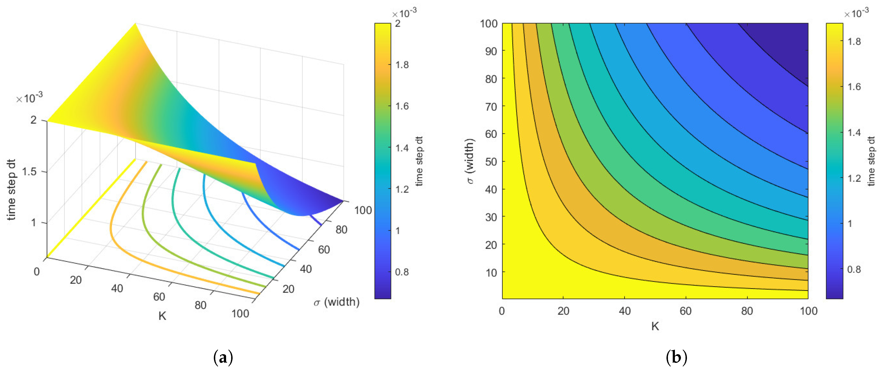
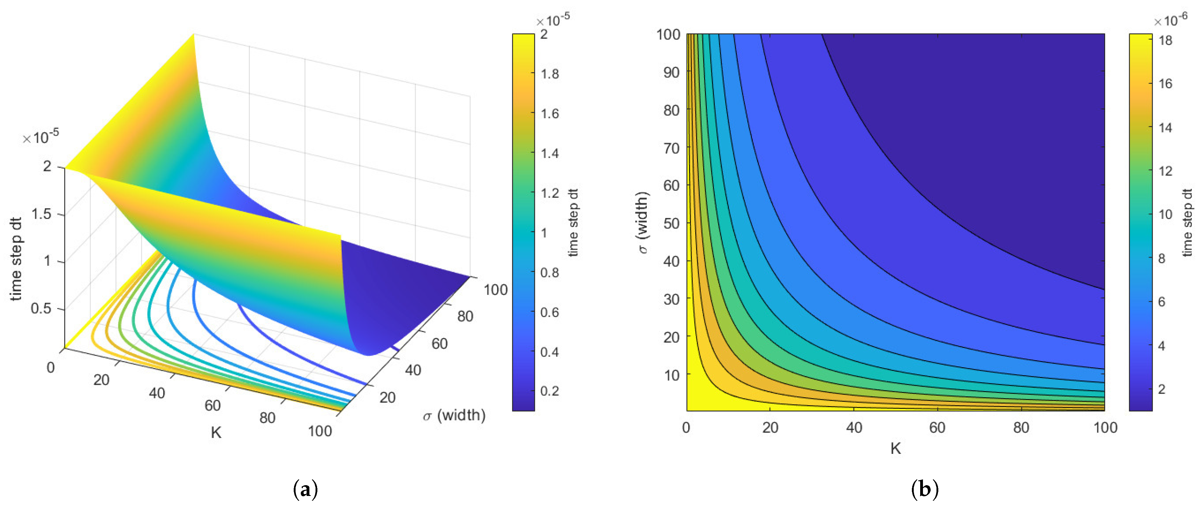
3.3.1. Stability at Interfaces

Note that, in order to ensure the positivity of the quantities in the above formulas deriving from the KK conditions—i.e., (48) for the 2D domain and (55) or (45) for the 1D domain—we also need to take care of the ratio between the KK coefficient K and the space discretization steps. In particular, for (48) and (45), one needs to ensure that K t x and, respectively, K t x y is not too big in order to damp possible high oscillations produced by the term in parentheses. Similarly, in (55) we need to check that K t x ( b a ) is small in order to prevent the growth of the negative term.
Moreover, as previously discussed, we need to check that the numerical monotonicity condition is satisfied:
k 1 k 2 + φ i , j n 2 | x , i , j n φ i , j n | D M
in the computational domain in order to ensure non-negative solutions.
Now, we consider the interface between the 2D and 1D domains. If we assume g = 0 and f = χ ( ϕ ) ϕ , the first equation in the 2D parabolic system, (8), rewrites as:
t u = D u d i v u · f .
The transmission condition (48) reads as:
u N x + 1 , j n + 1 = u N x + 1 , j n D u t x 2 δ x 1 ( u N x , j n + u N x , j n + 1 ) + D u t 2 y 2 δ y 2 u N x + 1 , j n + u N x + 1 , j n + 1 + t x f N x , j x , n u N x , j n + f N x + 1 , j x , n u N x + 1 , j n t 2 y f N x + 1 , j + 1 y , n u N x + 1 , j + 1 n f N x + 1 , j 1 y , n u N x + 1 , j 1 + t x | f N x , j x , n | u N x , j n | f N x + 1 , j x , n | u N x + 1 , j n + t 2 y | f N x + 1 , j + 1 y , n | u N x + 1 , j + 1 n 2 | f N x + 1 , j y , n | u N x + 1 , j n + | f N x + 1 , j 1 y , n | u N x + 1 , j 1 n + x t K u 0 c , n v N x + 1 , j n + u 0 c , n + 1 u N x + 1 , j n + 1 KK - transmission term .
Then, the transmission condition (55) for g = 0 and f = χ ( ϕ ) ϕ x now reads as:
u 0 c , n + 1 = u 0 c , n + D u c t x 2 δ x 1 u 0 c , n + u 0 c , n + 1 t x u 0 c , n f 0 n + u 1 c , n f 1 n + t x u 1 c , n | f 1 n | u 0 c , n | f 0 n | + x t K j = j a j b u N x + 1 , j n + u N x + 1 , j n + 1 ( b a ) u 0 n + u 0 n + 1 KK - transmission term
for j = j a , j b . For the transmission condition (58), we see that monotonicity is preserved when:
1 D u t x 2 D u t y 2 + t x f N x + 1 , j x , n t x | f N x + 1 , j x , n | t y | f N y + 1 , j y , n | t x K > 0 ,
which gives us the stability condition for the left side of the interface.
For the right side of the interface, if we assign the doubly parabolic 1D system (9), we have the stability condition:
1 D u c t x 2 + λ f c , 0 n t x | f 0 n | t x K ( b a ) .
We underline that (61) is not only influenced by the KK-constant K but also by the channel width σ : = ( b a ) , which must be taken care of accordingly.
Analogously, we conduct the derivation of stability conditions for the transmission conditions in the case where we assign the 2D parabolic model (57) on the left part of the interface and the hyperbolic system (10) on the right. For the sake of clarity, we rewrite the hyperbolic part of the system (10) for the density flux of individuals when we assume g = 0 :
t u c + x v c = 0 , t v c + λ c 2 x u c = F c .
The KK-transmission explicit version of conditions (46) and (45) in this case read as:
u 0 c , n + 1 = u 0 c , n + λ t x u 1 c , n u 0 c , n t x t 2 λ v 0 c , n + v 1 c , n t 2 λ F c , 0 n + F c , 1 n K t x y j = j a j b u 0 c , n u N x + 1 , j n + u 0 c , n + 1 u N x + 1 , j n + 1 , u N + 1 c , n + 1 = u N + 1 c , n + λ t x u N c , n u N + 1 c , n + t x t 2 λ v N c , n + v N + 1 c , n + t 2 λ F c , N n + F c , N + 1 n K t x y j = j a j b u N + 1 c , n u 0 , j c , n + u N + 1 c , n + 1 u 0 , j c , n + 1 , v 0 c , n = K ( b a ) u 0 c , n + K y j = j a j b u N x + 1 , j l , n + u N x + 1 , j l , n + 1 , v N + 1 c , n = K ( b a ) u N + 1 c , n + K y j = j a j b u N x + 1 , j r , n + u N x + 1 , j r , n + 1 .
In order to establish the monotonicity condition, as in [39], we need to diagonalize the boundary conditions above into the diagonal variables w 0 n + 1 , z 0 n + 1 , w N + 1 n + 1 , z N + 1 n + 1 with the relation u = w + z and v = λ z w .
We have:
v 0 c , n + 1 = λ z 0 c , n + 1 w 0 c , n + 1 = K ( b a ) ( z 0 c , n + 1 + w 0 c , n + 1 ) + K y j = j a j b u N x + 1 , j l , n + 2 + u N x + 1 , j l , n + 1 .
If we set ρ : = λ ( b a ) K λ + ( b a ) K , ς n + 1 : = + K λ + ( b a ) K j = j a j b u N x + 1 , j l , n + 2 + u N x + 1 , j l , n + 1 we find
z 0 n + 1 = ρ w 0 n + 1 + y ς n + 1
and
w 0 n + 1 + ρ w 0 n + 1 + ς n + 1 = ( 1 + ρ ) w 0 n + ς n + 2 λ t x w 1 n ρ w 0 n ς n + t 2 ρ 1 w 0 n + ς n + z 1 n w 1 n t 2 λ F c , 0 n + F c , 1 n t x K k ( ( b a ) 1 + ρ w 0 n + w 0 n + 1 + ( b a ) ς n + ς n + 1 j = j a k j b k u N x + 1 , j n + u N x + 1 , j n + 1 ) .
Now, by applying the monotonicity condition we get the following inequality:
1 + ρ 2 λ t x ρ + t 2 ρ 1 t x K ( b a ) 1 + ρ t 2 λ F c , 0 n > 0 t 1 + ρ 2 λ x ρ ρ 1 2 + K ( b a ) ( 1 + ρ ) x + F c , 0 n 2 λ
For the implicit AHO, the condition above reads as:
t 1 + ρ K ( b a ) ( 1 + ρ ) x + F c , 0 n 2 λ .
In Figure 3, the time step restriction (64) is depicted for a qualitative understanding of the effect of the Kedem–Katchalsky constant K and of the channel width σ on the time step t . As expected, the time step t must be chosen smaller when either K or σ increases. Furthermore for K = 0 we recover the time step restriction of the A H O 2 -scheme t 4 x x + 4 λ = 2 · 10 3 . Since the values of K are typically of similar magnitude to the diffusion coefficients, the additional stability restrictions caused by the hyperbolic part of the transmission conditions are minimal.
Finally, we also point out that the time step restriction for the transmission condition for the one-dimensional parabolic Equation (61) is much more severe than for the one-dimensional hyperbolic (64), which can also be seen qualitatively in the steepness of Figure 3 and Figure 4.
Comparing all time step restrictions (61) and (64) with each other, it is evident that the restriction for the two-dimensional parabolic transmission condition dominates the full model.
For the sake of completeness, we underline that at each time step a non-linear equation system must be solved, for which Newton–Krylov subspace methods [40] can be used, which take advantage of the mostly sparse structure of the Jacobian matrix.

4. Numerical Tests and Results

We start this section with a preliminary test on mass-preserving properties at the boundaries. Indeed, in absence of source terms, the masses of cells and chemical substances are preserved. Then, in order to perform a numerical verification of this property, we consider the numerical approximation at the interface between 1D-1D models in the next numerical example.
Example 1.
In Figure 5, a comparison between the central mass-preserving (24) and standard finite difference (23) boundary conditions is depicted, for the 1D-doubly parabolic case on both sides of the interface (on the left) and for the 1D-doubly parabolic-1D-hyperbolic-parabolic interface (on the right). From this 1D numerical example, the necessity of developing modified boundary conditions which are consistent and preserve the mass correctly is evident. We also underline that for the discretization of the Neumann condition, the forward scheme is first-order accurate, while the central scheme is second-order accurate; for more details, see [41].
From now on, this section is devoted to the presentation of the numerical tests and the parameters of the problem are reported in Table 1. Our aim is to show the ability of the simulation algorithm based on the model (3)–(7) to reproduce the qualitative behavior of the two population sharing the same habitat as observed in the videos of laboratory experiments, [1,2,25].
We remark that we decided to perform numerical simulations of the chip geometry by assigning the 1D-hyperbolic-parabolic model on channels, since it seems more realistic.
Example 2.
Before we numerically simulate the laboratory experiment with the algorithm, we conduct a simple numerical test in order to prove its accuracy. We assumed the following setting: a left squared chamber Ω l with one corridor positioned in the middle and only one cell family with initial distribution u ( x , y , 0 ) = 5 e 1 2 ( x 0.5 ) 2 + ( y 0.5 ) 2 . Since we do not have any analytical solution for this problem, we choose Δ t and Δ x = Δ y , which are small enough to obtain reasonable error estimations. In this case, we use d t = 10 4 and Δ x = Δ y = 5 × 10 4 for the approximation u e at time t = 100 and calculate the error as the quantity u e u approx in L 1 -norm.
In order to confirm the order of our scheme, we use a log-log-plot with constant and small enough Δ t (resp. Δ x ) and decreasing Δ x (resp. Δ t ). As shown in Figure 6 and Figure 7, the time order and space order are equal to line with slope 2 in the log-log plot, which corresponds to our scheme of order 2 in time and space.
Now, we describe the simulation of the chip environment. All the simulations were performed in MATLAB©. The computational time for a simulation on the complete geometry until time t = 50,000 took about 400 s on an Intel(R) Core(TM) i7-3630 QM CPU 2.4 GHz. The computational domain is schematized in Figure 2 with the two chambers and 5 corridors C m : = [ 0 , L ] , m = 1 , , 5 with the same width = 12 μ m and equispaced from each other. The numerical method implemented is listed in Section 3.3; for the 1D channels, the A H O 2 -scheme (of second order) is implemented, since there we are considering the hyperbolic-parabolic model. The discretization grid has time step size t = 100 s and space size x = 2.5 μ m , y = 25 μ m.
For the examples below, we assume the following initial condition (time t = 0 ) for the tumor cells distribution on the chip for ( x , y ) Ω l :
T ( x , y , 0 ) = 5 e 10 4 x 2 + ( y 500 ) 2 + 5 e 10 4 x 2 + ( y 5 ) 2 + 5 e 10 4 x 2 + ( y 1000 ) 2 ,
Whereas, in the corridors and the right chamber, no tumor cells are present.
For the immune cells distribution on the chip for ( x , y ) Ω r , we assign:
M ( x , y , 0 ) = 5 , for x , y Ω r ,
to mean that macrophages are disposed in the right chamber, whereas no immune cells are present in the left chamber nor in the corridors at the beginning.
For the chemoattractants, we set a constantly null initial density for ω and φ in both the chambers and also in the channels.
Example 3.
First scenario: treated case. For the following numerical simulation, we replicate the laboratory experiment of the first scenario (treated case) described in Section 2.1; see also [1]. All the parameters are reported in Table 1.
The results are depicted in the following Figure 8 and Figure 9.
In Figure 8 and Figure 9, we can see the density of the tumor cells T and macrophages M for different times t = 0 , t = 10000   s , and t = 50,000 s. Note that at time t = 0 tumor cells are present in the left chamber only and immune cells are present in the right chamber only.
Since tumor cells are previously treated by a chemoterapy drug, they slowly diffuse around and stay confined in the left chamber Ω l during all the simulation time; in the meanwhile they produce chemoattractant φ attracting immune cells. Immune cells M, instead, diffuse around in Ω r , cross the channels, and after a certain time they enter the left chamber Ω l while creating chemoattractant ω.
This is due to the fact that the chemoattractant φ produced by cancer cells travels through channels and induces a migration of the immune cells M towards the tumor cells T, causing a higher migration towards the center of the left chamber where the initial distribution of tumor cells was closest to the chambers, as we observe from the laboratory experiment.
At the final time t = 50,000 s, we can see that the quantity of tumor cells is decreasing under the action of immune cells producing chemokine ω.
Example 4.
Second scenario: untreated case.In this numerical test, we consider the second scenario where the tumor is not treated with any medicine. Therefore, in this case we assume a higher diffusion coefficient for the tumor, but the initial conditions are the same as those used above. The results are depicted in the following Figure 10.
In Figure 10, we can see the density of the tumor cells T and macrophages M for times t = 10,000 s and t = 50,000 s. Note that at time t = 0 tumor cells are present in the left chamber only and immune cells are present in the right chamber only.
Since, in the laboratory experiment, untreated tumor cells diffuse around, cross the channels, and enter the right chamber Ω r after some time, we try to reproduce such behavior by using a diffusion coefficient D T of a order of magnitude higher respect to the one used in the first scenario. Moreover, in this case the tumor cells do not produce chemoattractant φ; for this reason, here we set α ϕ = 0 . Immune cells M diffuse around in Ω r and do not cross the channels, since the chemical stimulus is not secreted by T cells. Moreover, the production of the chemical substance w is neglected in this case, thus tumor cells are not killed.
We only mention that we tested the 1D-doubly parabolic model on channels and compared it with the hyperbolic-parabolic model used in the previous examples. By using the same initial data as for the other examples, we notice that the doubly parabolic model seems to have a similar pattern as for the hyperbolic-parabolic model depicted above, but the scale of the quantities differs a lot between these models.
In particular, for the doubly parabolic model the concentration of the tumor cells T is two or three order of magnitude higher. This is due to the much slower movement of the immune cells through the channels. This also explains the much higher concentration of the chemoattractant ϕ because of the much higher concentration of T compared to in the other models.
In the following Figure 11, we represent the density of tumor cells and immune cells as particles, by randomly placing them according to their density. The higher the density at a given point, the more cells will be distributed randomly around that area. If the density is lower than a chosen threshold in a certain point, no cells will be represented around it.

5. Conclusions and Future Perspectives

The principal feature of the present work has been the development of a simulation tool to describe cell movements and interactions inside a microfluidic chip environment. Our study focused on both the modelling and the numerical point of view. Indeed, schematizing the chip geometry as two 2D boxes connected by a network of 1D channels, the main issues were:
  • the introduction of mass-preserving conditions involving the balancing of incoming and outgoing fluxes passing through interfaces between 2D and 1D domains;
  • the development of mass-preserving numerical schemes at the boundaries of the 2D domain and the mass-preserving transmission conditions at the 2D–1D interfaces.
Furthermore, from the modelling point of view, we studied the dynamics in the channels in the case of a doubly parabolic model and a hyperbolic-parabolic model. Since we obtained comparable asymptotic states, we decided to apply the hyperbolic-parabolic model in order to obtain a finite speed of propagation in the channels, which seems to be more realistic. In this framework, bearing in mind the laboratory experiments on a chip described in Section 2.1, it was possible to simulate the chip environment with two species of living cell moving in it. Moreover, we remark that we can simulate more complicated situations where more than two cell species are present.
As a further development of the present study, we will work on the calibration of the model against experimental data obtained from cell tracking in a microfluidic chip [1,2,25].

Author Contributions

Methodology, G.B. and R.N.; Software, E.C.B.; Supervision, G.B. and R.N.; Validation, E.C.B. and G.B.; Visualization, E.C.B.; Data curation, E.C.B. and G.B.; Conceptualization, R.N.; Investigation, E.C.B. and G.B. Writing, E.C.B. and G.B. All authors have read and agreed to the published version of the manuscript.

Funding

This research received no external funding.

Institutional Review Board Statement

Not applicable.

Informed Consent Statement

Not applicable.

Data Availability Statement

All data are contained within the article.

Conflicts of Interest

The authors declare no conflict of interest.

References

  1. Vacchelli, E.; Ma, Y.; Baracco, E.E.; Sistigu, A.; Enot, D.P.; Pietrocola, F.; Yang, H.; Adjemian, S.; Chaba, K.; Semeraro, M.; et al. Chemotherapy-induced antitumor immunity requires formyl peptide receptor 1. Science 2015, 350, 972–978. [Google Scholar] [CrossRef]
  2. Businaro, L.; De Ninno, A.; Schiavoni, G.; Lucarini, V.; Ciasca, G.; Gerardino, A.; Belardelli, F.; Gabriele, L.; Mattei, F. Cross talk between cancer and immune cells: Exploring complex dynamics in a microfluidic environment. Lab. Chip 2013, 13, 229–239. [Google Scholar] [CrossRef]
  3. Parlato, S.; De Ninno, A.; Molfetta, R.; Toschi, E.; Salerno, D.; Mencattini, A.; Romagnoli, G.; Fragale, A.; Roccazzello, L.; Buoncervello, M.; et al. 3D Microfluidic model for evaluating immunotherapy efficacy by tracking dendritic cell behaviour toward tumor cells. Sci. Rep. 2017, 7, 1–16. [Google Scholar] [CrossRef] [PubMed]
  4. Keller, E.F.; Segel, L.A. Initiation of slime mold aggregation viewed as an instability. J. Theor. Biol. 1970, 26, 399–415. [Google Scholar] [CrossRef]
  5. Greenberg, J.M.; Alt, W. Stability results for a diffusion equation with functional drift approximating a chemotaxis model. Trans. Am. Math. Soc. 1987, 300, 235–258. [Google Scholar] [CrossRef]
  6. Di Russo, C. Analysis and Numerical Approximation of Hydrodynamical Models of Biological Movements. Ph.D. Thesis, Roma Tre University (Università degli studi Roma Tre), Rome, Italy, 2011. [Google Scholar]
  7. Dolak, Y.; Hillen, T. Cattaneo models for chemosensitive movement. Numerical solution and pattern formation. J. Math. Biol. 2003, 46, 153–170, Corrected Version after misprinted p.160 in J. Math. Biol. 2003, 46, 461–478. [Google Scholar] [CrossRef]
  8. Filbet, F.; Laurençot, P.; Perthame, B. Derivation of hyperbolic models for chemosensitive movement. J. Math. Biol. 2005, 50, 189–207. [Google Scholar] [CrossRef] [Green Version]
  9. Gamba, A.; Ambrosi, D.; Coniglio, A.; De Candia, A.; Di Talia, S.; Giraudo, E.; Serini, G.; Preziosi, L.; Bussolino, F. Percolation, morphogenesis, and Burgers dynamics in blood vessels formation. Phys. Rev. Lett. 2003, 90, 118101.1–118101.4. [Google Scholar] [CrossRef] [Green Version]
  10. Perthame, B. Transport Equations in Biology, Frontiers in Mathematics; Birkhäuser: Basel, Switzerland, 2007. [Google Scholar]
  11. Serini, G.; Ambrosi, D.; Giraudo, E.; Gamba, A.; Preziosi, L.; Bussolino, F. Modeling the early stages of vascular network assembly. Embo J. 2003, 22, 1771–1779. [Google Scholar] [CrossRef] [Green Version]
  12. Bretti, G.; Gosse, L. Diffusive limit of a two-dimensional well-balanced approximation to a kinetic model of chemotaxis. In SN Partial Differential Equations and Applications; Springer: Berlin, Germany, 2021. [Google Scholar] [CrossRef]
  13. Guarguaglini, F.R.; Mascia, C.; Natalini, R.; Ribot, M. Stability of constant states and qualitative behavior of solutions to a one dimensional hyperbolic model of chemotaxis. Discret. Contin. Dyn. Syst. Ser. B 2009, 12, 39–76. [Google Scholar] [CrossRef]
  14. Natalini, R.; Ribot, M. An asymptotic high order mass-preserving scheme for a hyperbolic model of chemotaxis. SIAM J. Numer. Anal. 2012, 50, 883–905. [Google Scholar] [CrossRef] [Green Version]
  15. Gosse, L. Asymptotic-preserving and well-balanced schemes for the 1D Cattaneo model of chemotaxis movement in both hyperbolic and diffusive regimes. J. Math. Anal. Appl. 2012, 388, 964–983. [Google Scholar] [CrossRef]
  16. Gosse, L. Well-balanced numerical approximations display asymptotic decay toward Maxwellian distributions for a model of chemotaxis in a bounded interval. SIAM J. Sci. Comput. 2012, 34, A520–A545. [Google Scholar] [CrossRef] [Green Version]
  17. Bretti, G.; Natalini, R. Numerical approximation of nonhomogeneous boundary conditions on networks for a hyperbolic system of chemotaxis modeling the physarum dynamics. J. Comput. Methods Sci. Eng. 2018, 18, 85–115. [Google Scholar] [CrossRef] [Green Version]
  18. Bretti, G.; Natalini, R.; Ribot, M. A hyperbolic model of chemotaxis on a network: A numerical study. Math. Model. Numer. Anal. 2014, 48, 231–258. [Google Scholar] [CrossRef] [Green Version]
  19. Borsche, S.; Göttlich, S.; Klar, A.; Schillen, P. The scalar Keller-Segel model on networks. Math. Model. Methods Appl. Sci. 2014, 24, 221–247. [Google Scholar] [CrossRef]
  20. Kedem, O.; Katchalsky, A. Thermodynamic analysis of the permeability of biological membrane to non-electrolytes. Biochim. et Biophysica Acta 1958, 27, 229–246. [Google Scholar] [CrossRef]
  21. Quarteroni, A.; Veneziani, A.; Zunino, P. Mathematical and numerical modeling of solute dynamics in blood flow and arterial walls. SIAM J. Num. Anal. 2002, 39, 1488–1511. [Google Scholar] [CrossRef] [Green Version]
  22. Serafini, A. Mathematical Models for Intracellular Transport Phenomena. Ph.D. Thesis, “Sapienza” University of Rome 1, Rome, Italy, 2007. [Google Scholar]
  23. Cangiani, A.; Natalini, R. A spatial model of cellular molecular trafficking including active transport along microtubules. J. Theor. Biol. 2010, 267, 614–625. [Google Scholar] [CrossRef] [Green Version]
  24. Di Costanzo, E.; Ingangi, V.; Angelini, C.; Carfora, M.F.; Carriero, M.V.; Natalini, R. A Macroscopic Mathematical Model For Cell Migration Assays Using A Real-Time Cell Analysis. PLoS ONE 2016, 11, e0162553. [Google Scholar] [CrossRef]
  25. Agliari, E.; Biselli, E.; De Ninno, A.; Schiavoni, G.; Gabriele, L.; Gerardino, A.; Mattei, F.; Barra, A.; Businaro, L. Cancer-driven dynamics of immune cells in a microfluidic environment. Sci. Rep. 2014, 4, 6639. [Google Scholar] [CrossRef]
  26. Lucarini, V.; Buccione, C.; Ziccheddu, G.; Peschiaroli, F.; Sestili, P.; Puglisi, R.; Mattia, G.; Zanetti, C.; Parolini, I.; Bracci, L.; et al. Combining Type I Interferons and 5-Aza-2’-Deoxycitidine to Improve Anti-Tumor Response against Melanoma. J. Investig. Dermatol. 2017, 137, 159–169. [Google Scholar] [CrossRef] [PubMed] [Green Version]
  27. Nguyen, M.; De Ninno, A.; Mencattini, A.; Mermet-Meillon, F.; Fornabaio, G.; Evans, S.S.; Cossutta, M.; Khira, Y.; Han, W.; Sirven, P.; et al. Dissecting Effects of Anti-cancer Drugs and Cancer-Associated Fibroblasts by On-Chip Reconstitution of Immunocompetent Tumor Microenvironments. Cell Rep. 2018, 25, 3884–3893. [Google Scholar] [CrossRef] [Green Version]
  28. Altrock, P.M.; Liu, L.L.; Michor, F. The mathematics of cancer: Integrating quantitative models. Nat. Rev. Cancer 2015, 15, 730–745. [Google Scholar] [CrossRef] [PubMed]
  29. Emako, C.; Gayrard, C.; Buguin, A.; de Almeida, L.N.; Vauchelet, N. Traveling Pulses for a Two-Species Chemotaxis Model. PLoS Comput. Biol. 2016, 12, 1–22. [Google Scholar] [CrossRef]
  30. Preziosi, L.; Tosin, A. Multiphase and Multiscale Trends in Cancer Modellings. Math. Model Nat. Phenom. 2009, 4, 1–11. [Google Scholar] [CrossRef] [Green Version]
  31. Méhes, E.; Vicsek, T. Collective motion of cells: From experiments to models. Integr. Biol. 2014, 6, 831–854. [Google Scholar] [CrossRef] [Green Version]
  32. Di Costanzo, E.; Natalini, R.; Preziosi, L. A hybrid mathematical model for self-organizing cell migration in the zebrafish lateral line. J. Math Biol. 2015, 71, 171–214. [Google Scholar] [CrossRef] [Green Version]
  33. Murray, J.D. Mathematical Biology II Spatial Models and Biomedical Applications; Springer: Berlin/Heidelberg, Germany, 2003. [Google Scholar]
  34. Lapidis, I.R.; Schiller, R. Model for the chemotactic response of a bacterial population. Biophys. J. 1976, 16, 779–789. [Google Scholar] [CrossRef] [Green Version]
  35. Natalini, R. Convergence to equilibrium for the relaxation approximations of conservation laws. Comm. Pure Appl. Math. 1996, 49, 795–823. [Google Scholar] [CrossRef]
  36. Patankar, S.V. Numerical Heat Transfer and Fluid Flow; McGraw-Hill: New York, NY, USA, 1996; ISBN 0-89116-522-3. [Google Scholar]
  37. Crank, J.; Nicolson, P. A practical method for numerical evaluation of solutions of partial differential equations of the heat conduction type. Proc. Camb. Phil. Soc. 1947, 43, 50–67. [Google Scholar] [CrossRef]
  38. Hairer, E.; Wanner, G. Solving ordinary differential equations. II, vol. 14 of Springer Series in Computational Mathematics. In Stiff and Differential-Algebraic Problems, 2nd revised ed.; Springer: Berlin, Germany, 2010. [Google Scholar]
  39. Aregba-Driollet, D.; Natalini, R. Convergence of relaxation schemes for conservation laws. Appl. Anal. 1996, 61, 163–193. [Google Scholar] [CrossRef]
  40. Knoll, D.A.; Keyes, D.E. Jacobian-Free Newton-Krylov methods: A survey of approaches and applications. J. Comput. Phys. 2004, 193, 357–397. [Google Scholar] [CrossRef] [Green Version]
  41. Morton, K.W.; Mayers, D. Numerical Solutions of Partial Differential Equations; Cambridge University Press: Cambridge, UK, 2005. [Google Scholar]
  42. Curk, T.; Marenduzzo, D.; Dobnikar, J. Chemotactic Sensing towards Ambient and Secreted Attractant Drives Collective Behaviour of E. coli. PLoS ONE 2013, 8, e74878. [Google Scholar] [CrossRef] [PubMed] [Green Version]
Figure 1. Microfluidic chip environment: two chambers connected by multiple channels. Credits by Vacchelli et al. [1] edited by AAAS.
Mathematics 09 00688 g001
Figure 2. Simplified schematization of the chip geometry depicted in Figure 1.
Mathematics 09 00688 g002
Figure 3. Time step restriction (64) t for the hyperbolic transmission condition with x = 0.01 , y = 0.1 and λ = 5 for different K and channel widths ( b a ) for the transmission between the two-dimensional parabolic Equation (57) with the one-dimensional hyperbolic Equation (62) with f = 0 .
Mathematics 09 00688 g003
Figure 4. Time step restriction (61) t for the one-dimensional parabolic transmission condition with x = 0.01 , y = 0.1 and D = 5 for different K and channel width σ = b a , f = 0 . As expected, the time step t must be chosen smaller when either K or the channel width σ increases.
Mathematics 09 00688 g004
Figure 5. (left) evolution of total mass for 1D-1D-doubly parabolic model with standard vs. mass-preserving boundary conditions. (right) evolution of total mass for 1D-1D-hyperbolic-parabolic model with standard vs. mass-preserving boundary conditions.
Mathematics 09 00688 g005
Figure 6. Log-log plot of the error—namely, the quantity u e u approx in L 1 -norm as a function of the space step, with fixed Δ t = 10 3 and decreasing Δ x = 0.5 , 0.1 , 0.05 , 0.001 at time t = 100 . We depict in blue the obtained error and in red a line with slope 2 for comparison.
Mathematics 09 00688 g006
Figure 7. Log-log plot of the error, namely the quantity u e u approx in L 1 -norm as a function of the time step, with fixed Δ x = 10 3 and decreasing Δ t = 0.5 , 0.1 , 0.05 , 0.001 at time t = 100 . We depict in blue the obtained error and in red a line with slope 2 for comparison.
Mathematics 09 00688 g007
Figure 8. Treated case. Initial distribution for the model (3)–(7) at time t = 0 .
Mathematics 09 00688 g008
Figure 9. Treated case. Evolution of the model (3)–(7) at time t = 10,000 s (top) and at time t = 50,000 s (bottom).
Mathematics 09 00688 g009
Figure 10. Untreated case. Evolution of the model (3)–(7) at time t = 10,000 s (top) and at time t = 50,000 s (bottom).
Mathematics 09 00688 g010
Figure 11. Visualization of immune cells (blue dots) and tumor cells (red squares) for times t = 0, t = 5, and t = 50 using the density of each quantity and representing them as cells.
Mathematics 09 00688 g011
Table 1. Parameters of the problem.
ParameterDescriptionUnitsValueRef.
D M Diffusivity of cells μ m 2 /s 9 × 10 2  [33]
D T Diffusivity of T -scenario 2 μ m 2 /s 56 × 10 1 empirical
D T Diffusivity of T -scenario 1 μ m 2 /s 5.6 × 10 1  [33]
D φ , D ω Diffusivity of chemoattractants μ m 2 /s 2 × 10 2  [33]
α φ growth rate of φ in scenario 2s 1 /cell0empirical
α φ growth rate of φ for scenario 1s 1 /cell 0.5 × 10 1  [42]
β φ consumption rate of φ s 1 10 4  [42]
α ω growth rate of ω for scenario 1s 1 /cell 10 1  [42]
α ω growth rate of ω for scenario 2s 1 /cell0empirical
β ω consumption rate of ω s 1 10 4 [42]
k 1 cellular drift velocitymol cm 2 s 1 3.9 × 10 9  [33]
k 2 receptor dissociation constantmol 5 × 10 6  [33]
Smaximum secretion rate of the chemicalsg/ μ m 3 1.9676 × 10 11  [33]
γ equivalent Michaelis constantcells / μ m 3 10 4  [33]
Llength of the corridor μ m500datum
L x horizontal size of the box μ m100datum
L y vertical size of the box μ m1000datum
KKedem–Katchalsky constant-500empirical
Publisher’s Note: MDPI stays neutral with regard to jurisdictional claims in published maps and institutional affiliations.

