
Handling Hysteresis in a Referral Marketing Campaign with Self-Information. Hints from Epidemics

Department of Electrical and Information Engineering, University of Cassino and Southern Lazio, Di Biasio Str., I-03043 Cassino, Italy
Mathematics 2021, 9(6), 680; https://doi.org/10.3390/math9060680
Submission received: 6 February 2021
/
Revised: 14 March 2021
/
Accepted: 18 March 2021
/
Published: 22 March 2021
(This article belongs to the Special Issue Differential Equation Models in Applied Mathematics: Theoretical and Numerical Challenges)
Abstract
:In this study we show that concept of backward bifurcation, borrowed from epidemics, can be fruitfully exploited to shed light on the mechanism underlying the occurrence of hysteresis in marketing and for the strategic planning of adequate tools for its control. We enrich the model introduced in (Gaurav et al., 2019) with the mechanism of self-information that accounts for information about the product performance basing on consumers’ experience on the recent past. We obtain conditions for which the model exhibits a forward or a backward phenomenology and evaluate the impact of self-information on both these scenarios. Our analysis suggests that, even if hysteretic dynamics in referral campaigns is intimately linked to the mechanism of referrals, an adequate level of self-information and a fairly high level of customer-satisfaction can act as strategic tools to manage hysteresis and allow the campaign to spread in more controllable conditions.
1. Introduction and Motivations
In the last century, mathematical models based on differential equations have been fruitfully applied to describe phenomena belonging to even extremely different disciplinary fields. As well known in literature [1], mathematical models can act essentially in two directions: those based on more sophisticated mathematical tools can give a great contribution in terms of quantitative predictions but simpler qualitative models can be precious to shed light on the constitutive mechanisms, highlighting their role and reciprocal interactions.
Precisely because they go to the heart of the phenomena, simple mechanistic qualitative models are capable to create bridges between apparently very distant worlds, making sure that models and methodologies used in a certain context could be exploited to open the way to the understanding of phenomena that are similar in their underlying mechanisms. On this line, it is not surprising that the simple mechanistic model found by Volterra [2] to describe the interaction between preys and predators in the Italian Adriatic Sea displays the same mathematical structure as the one introduced in those same years by Lotka [3] in the context of the chemical kinetics. And, again, it is not surprising at all that a discipline such as marketing has been able to benefit from the models and the modus operandi of mathematical epidemiology. In this case, the unifying factor is the idea of contagion, a key mechanism for those forms of marketing defined as viral. The viral name refers in particular to all those marketer-initiated consumer activities that spreads a marketing message unaltered across a market or segment in a limited time period mimicking an epidemic [4]. Terms from epidemiology have been hence widely used to explain such viral marketing process [5,6].
This interconnection has become even more pronounced with the unchallenged emergence of new means of communication. With consumers showing increasing resistance to traditional forms of advertising, marketers have been forced to rely on alternative strategies. Among these are social networks, whose usage is sensitively growing among marketing managers with the aim to promote an idea, a product or a brand at no additional cost to the firm. If a marketer encourages consumers to share and spread a marketing message through their social contacts, this is called Referral Marketing [7]. In few words, referral marketing spreads the word about a product or service through a business’ existing customers, rather than traditional advertising. This kind of marketing uses referrals or word-of-mouth to promote services or products and businesses may control it through suitable strategies and make a viral referral campaign. Strategic use of referral marketing can hence allow marketers to leverage the power of consumer recommendations in order to achieve the desired results. On this line, questions as ‘Which are the underlying set of interactions that ensure a marketing message to go viral? Which parameters can allow an effective spread of a marketing message through a viral process?’ becomes simply crucial. And since a viral marketing message involves a person-to-person transmission spreading within a population just like an epidemic, it is not strange that the most likely enlightening answers could hence come from epidemic models.
In the classical models of epidemiology, the interactions between susceptible and infected is a key factor for the spread of an epidemic, qualitatively defined as a situation in which the number of the infected reaches a significant percentage at steady state. In the case of a viral marketing campaign it can be thought as a situation for which, because of the sharing mechanisms, the marketing message reaches and attracts a majority of its target consumers. Obviously in epidemiology one aims to contain epidemics whereas, within the marketing framework, the main purpose is to maximize the spread.
In the context of online social networks and digital contagion, many efforts have recently been made to model such kind of dynamics: reference [4] discussed the viral marketing diffusion within the SIR and SEIAR epidemic framework and reference [8] proposed a mathematical model borrowed from epidemiology to describe its spread. An extensive survey in [9] underlined that along with the viral component, a particular focus on customer behaviors should be given to ensure the relevance and survival of a newly-launched campaign. On this line, references [7,10] considered more realistic models for the viral campaign spread, where specific behavioral factors were introduced to take into account a customer’s perspective about marketing messages, i.e., inherent adversion, brand trust, remembering and reminding.
In this paper we want to pursue this line focusing on the interplay between two behavioral mechanisms that can be involved together in a referral campaign. In fact, if referral is obviously the key mechanism of a referral campaign, it is not the only one. The Nielson Global Survey of Trust in Advertising [11] clearly supports the remarkable potential of referrals showing that for the question ‘To what extent do you trust the following form of advertising?’, the answer ‘Recommendation from the people I know’ gains the first position with 83%. But the answer ‘Consumer’s opinion posted online’ is also on the podium with , confirming how online reviews remain a trust source of customer information. This means that, on average, two-thirds of consumers feels the need of ‘self-information’ and make purchases after inspecting customers’ opinions posted online about a particular product or service. In this case information comes from sources of reviews with no conflicts of interest, such as specific consumers’ forum that collect opinions by those who bought particular products or experienced certain services.
Therefore in a referral marketing campaign, the nature of the information for the potential consumer can be twofold: passive, when it is linked to the mechanism of recommendations by friends and acquaintances or active when it is linked to the self-information mechanism described above. Our aim is to elucidate under what conditions the interplay between ‘passive’ and ‘active’ information can strengthen or weaken the survival chances of a referral campaign. On this line, we enrich the model introduced in [10] with the mechanism of self-information that accounts for information about the product performance basing on consumer’s experience on the recent past. Such a mechanism, based on a kind of learning that a potential consumer can adopt during the referral campaign, is mathematically obtained by introducing a distributed lag in the population equations that therefore become an integro-differential system, i.e., a delay differential model. The importance of considering such kind of models is provided by the fact that the role of delays in biological [12,13,14,15] as well as in economic models [16,17,18,19,20] is widely recognized, being often appropriate for these kind of problems to allow the rate of change of the system variables to depend in some sense on the previous history. We want to establish conditions for which the model exhibits a forward or a backward phenomenology and evaluate the impact of self-information on both these scenarios. The backward phenomenology, in particular, is connected to a situation of bistability between the campaign-free equilibrium and the campaign-standing equilibrium and can lead the system towards hysteresis-type behaviors. In a very qualitative way the term hysteresis, related to the idea of “irreversibility”, denotes the effects that persist after the causes that determined them have been removed. The relevance of using hysteresis at economic systems level is well recognized and marketing provides a generous framework to improve the understanding of this phenomenon in the economic sphere. In marketing, hysteresis is mainly thought in relation to consumer behaviour as well as to temporary or permanent changes of consumption patterns caused by specific marketing tools [21,22,23].
Its link with hysteresis is the reason why, in mathematical epidemiology, many papers have been focused on backward bifurcation, i.e., [24,25,26,27,28]. In that context, the basic reproduction number is usually defined as the expected number of new infections produced by a single infective individual introduced into a disease-free population [29] and represents the threshold value that separates the stability and instability regimes of the disease-free equilibrium. There are two bifurcation scenarios commonly detectable at : (i) forward bifurcation that implies disease eradication below the threshold ; (ii) backward bifurcation that includes a saddle-node (sn) bifurcation at along with a subcritical transcritical bifurcation at ; it involves a multiplicity of endemic equilibria and subcritical persistence of the disease. When a backward scenario is found, reducing below 1 is not sufficient to eradicate the disease and a further effort should be done until is lowered below the critical value . It is therefore obvious that, in epidemic models, detecting and managing the occurrence of backward bifurcations are two features of primary importance in the perspectives of the disease control. In viral marketing, however, the backward scenario may play a different role than in epidemics since it could be seen as an opportunity for the firm to carry on the viral campaign even in adverse conditions, which in itself adds an interesting perspective to the problem. Also in this case, however, the backward scenario must still be carefully monitored because in the bistability regime, too large displacements from the campaign-standing equilibrium can bring the system into the basin of attraction of the campaign-free equilibrium. That means a sudden collapse of the referral campaign.
The paper is structured as follows: In Section 2, we enrich the model introduced in [10] with the mechanism of self-information by the means of a variable that summarizes information about the product performance basing on consumers’ experience on the recent past. In Section 3 we get conditions for the existence of a campaign-free and of a campaign-standing equilibria and establish under which conditions, expressed as a function of the system parameters, the campaign spread goes towards stopping. In Section 4 a bifurcation analysis in the neighbouring of the campaign-free equilibrium is performed and conditions are obtained for the emergence of a forward or a backward scenario that are also discussed in the perspective to improve the sustainability of the referral campaign. The effects of self-information on the bifurcation thresholds is shown in Section 5 where the role of the customer satisfaction parameter is also elucidated. Concluding remarks, in Section 6, close the paper.
2. A Referral Marketing Model with Self-Information
To mimics referral dynamics, a model was introduced in [7] with the total population divided in three mutually exclusive subpopulations: Unaware, Broadcaster and Inert. The unaware class U is the target market, namely ‘susceptible’ people that have not yet received the message about a certain product but are exposed and have a chance of receiving it; the broadcaster class B is composed of individuals who have received the message earlier and have the potential to spread the message further to their social contacts; the inert class I is instead made of individuals that, willingly or unwillingly, do not take part in the campaign even if they have come across it at least once. This model is essentially based on contagion as the basic transition mechanism between different subgroups.
To increase the degree of realism, the authors then proposed in [10] a more realistic model including some additional features raised in a survey campaign developed in [9]. Analyzing the surveys and the interactions between different people, they modeled the transition between different sub-groups with taking into account some additional factors that more clearly reflect customer’s perspective about marketing messages: (a) inherent aversion, i.e., a portion of individuals could be strongly against the mechanisms of referral marketing in general; (b) brand trust, i.e., people need to ‘trust’ the person who is referring the product (for example family or friends) as well as the brand-names while participating in referral marketing; (c) remembering and reminding, i.e., strategically designed emails from the company or casual reminders from friends can tempt inert individuals to become broadcasters again. The following model was hence considered [10]:
where u,b and i are the fraction of the unaware, broadcaster and inert classed normalized by the total population. In (1), it is assumed that a broadcaster spreads the message to a member from unaware class at a rate and, whenever a broadcaster sends the referral message to an unaware individual, this moves to the broadcaster class with a probability p and to the inert class with a probability . The parameter assumes a high value if the campaign comes from a trusted brand or the message comes from a trusted member and can be hence interpreted as the ‘trust’ parameter. The term accounts that some individuals of the unaware class might decide to ignore the messages or to not take part in the campaign, i.e., groups of individuals that are for example rigidly inert. Messages from not so trustworthy brand or members increases the value of .
Once the unawares have become broadcasters or inert, they can ‘change their mind’ by moving from one class to another respectively. In fact, broadcasters can stop sharing the message, hence moving to the inert class at a rate . On the other hand, inert people can move back to broadcaster class following two different mechanisms: (i) independently of their interaction with other individuals (like reminder from the company etc.) at a rate or (ii) because of their interaction with another broadcaster (like reminder from a friend, discussion with family members) at a rate where is the original relapse rate and p is the trust parameter. Obviously people can join or leave a particular social platform where the campaign is going. It is then assumed a constant input in the unaware class and a natural ‘mortality rate’ for each class so that a fixed population size can be maintained.
The analysis carried out in [10] showed that the brand loyalty and brand name are two important factors to create positive reaction of a person towards a campaign message. Moreover, model dynamics turned out to be critically affected by variations in the relapse rate that was recognized to be crucial to safeguard the survival of the campaign. In particular, sufficiently high values of the relapse rate could drive the system towards a bistability situation between the campaign-free and the campaign-standing equilibria.
In [10] the involved information mechanism was essentially passive because the spread of the message is based on referrals. To investigate the role of an active information on the spreading of the referral campaign, we equipped model (1) with a self-information variable m that summarizes information about the product performance basing on the customers’ experiences in the recent past, i.e., online customer reviews. Because of this ‘active’ information process, we assume that unaware individuals can exit their class at a rate , moving to the broadcaster class with a probability q and to the inert class with a probability . The parameter assumes a high value if the online reviews on the product indicates an overall high level of satisfaction and can be hence interpreted as a ‘customer satisfaction’ parameter. We hence consider the following model:
where the self-information variable m is given by
The distributed lag (3) in the governing equations means that unaware, broadcaster and inert individuals at time t are affected by the state variables u, b, i at possibly all previous times in a way prescribed by the function and distributed in the past by the delay kernel which is also called ‘memory function’.
We assume here that the function where k is a positive parameter. Among the possible types of delay kernels, we consider
which qualitatively represents a weak delay in the sense that the maximum (weighted) response of the growth rate is to current population density whereas past densities have exponentially decreasing influence. Such a kernel provides therefore a reasonable effect of short term memory.
With (4) as delay kernel and by applying the linear chain trick [30], the set of delay differential Equations (2) and (3) turns out to be equivalent to the following set of ordinary differential equations that will be hereafter the object of our investigations:
with .
In the next section, we get conditions for the existence of a campaign-free and of a campaign-standing equilibria and establish under which conditions, expressed as a function of the system parameters, the campaign goes viral or is forced to stop.
3. The Campaign-Free and the Campaign-Standing Equilibria
Model (5) always admits a campaign-free equilibrium and, under suitable conditions on the system parameters can admit one or two campaign-standing equilibrium where:
and is a positive solution of the following algebraic equation,
with
and
By (6), it follows that is a positive equilibrium provided is a positive solution of (7). Moreover being (7) a second order algebraic equation we observe that, for certain ranges of the parameter values, model (5) could admit a multiplicity of campaign-standing equilibria.
In the next we assume so that the natural “mortality rate” for each class is considered slow with respect to the marketing process. Under this condition, both and are positive quantities. We now determine the conditions for which model (5) can admit feasible (i.e. positive) campaign-standing equilibria. To do that, we inspect the discriminant of the algebraic Equation (7), namely
and observe that, if , then (10) is a positive quantity so that by the Descartes’ rule of signs, the algebraic Equation (7) admits only one positive real solution. On the contrary, if , then where
and
For , is a positive quantity and it is also easy to prove that . We can hence conclude that: if then Equation (7) admits no real solutions; if then, by the Descartes’ rule of signs, the algebraic Equation (7) admits two negative real solutions; if then it admits two positive real solutions.
The above results can be summarized in the following theorems:
Theorem 1.
Let and . Then model (5) admits the campaign-free equilibrium and one positive campaign-standing equilibrium .
Theorem 2.
Let and . Then model (5) admits thecampaign-freeequilibrium and (i) if , none positive campaign-standing equilibrium exists; (ii) if , two positive campaign-standing equilibria exist.
As far as the local stability properties of the campaign-free equilibrium are concerned, we observe that the Jacobian matrix of model (5) when evaluated at , is given by
and admits as an eigenvalue. To reason about the sign of the other three eigenvalues, we introduce the following matrices:
and recall that the remaining three eigenvalues of have negative real part if and only if the following conditions holds:
We get and so that:
where is given in (9) and . We also observe that
and
that is always verified. Therefore for , the threshold quantity is negative so that for every positive value of a. Moreover by straightforward algebra follows that, for , inequality is always verified. We are hence in the position to state the following theorem:
Theorem 3.
Let . (i) If then the campaign-free equilibrium is unstable. (ii) If then the campaign-free equilibrium is locally asymptotically stable.
In the following section, we analyze in more details the nature of the transcritical bifurcation at and its impact on the sustainability of the referral campaign.
4. Sustaining the Campaign: Forward or Backward Scenario?
Within the epidemic framework, backward scenarios have been mainly detected by the means of specific bifurcation approaches [31] with the aim to establish the nature of the bifurcation at . Once the backward scenario is detected, the subcritical persistence of the disease can be prevented by varying significant parameters in the system or by the means of error-based methods as the Z-type control approach [32,33,34].
In this section, we discuss the occurrence of the backward vs the forward phenomenology for model (5), by using the method proposed in [35] that provides simple and manageable conditions for monitoring both these scenarios.
As shown in the previous section, is a transcritical bifurcation threshold. We observe that all the coefficients in the equilibrium Equation (7) may be regarded as functions of the parameter . Moreover at , so that Equation (7) becomes
and admits the roots and . The former is related to the campaign-free equilibrium and the latter corresponds to a positive campaign-standing equilibrium only if and have opposite signs. Therefore, in order to have a positive campaign-standing equilibrium, must hold. By implicit differentiation of Equation (7) with respect to , one obtains:
Now, looking at the equilibrium , at one has:
since, recalling (8), it holds . Therefore, in order inequality (12) to be verified, and must have opposite sign. This means that the slope of the bifurcation curve at must have opposite sign with respect to the coefficient . Since in our case a forward scenario at is obtained when and a backward scenario when , it hence follows that: (i) if then a backward bifurcation occurs at ; (ii) if , the system displays a forward bifurcation at .
For model (5), is hence a necessary and sufficient condition for the occurrence of the backward bifurcation at . By (9), the threshold depends on the parameter . Therefore by introducing,
where
the following result holds:
Theorem 4.
Proof.
It follows from (8) by direct computations. □
Remark 1.
It easy to prove by direct computation that the threshold defined in (11) is such that
so that results in Theorem 4 are in perfect agreement with the existence results provided in Theorem 2.
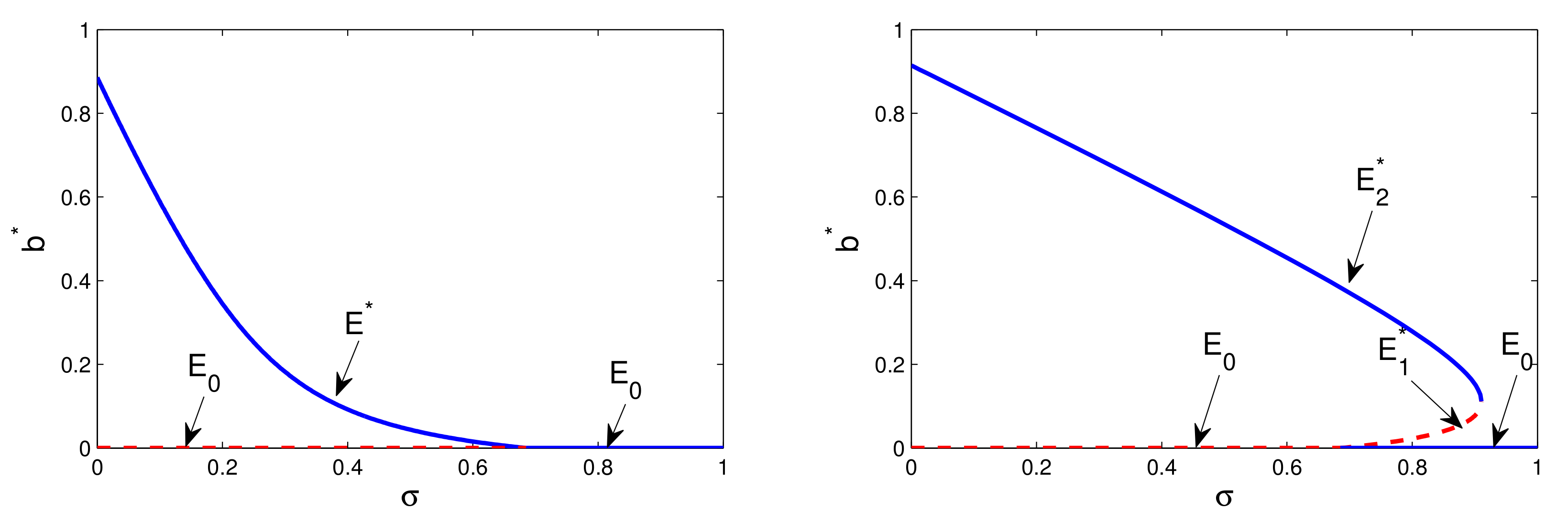
To validate the results found in Theorem 4, we show the local dynamics in the neighboring of the bifurcation value by the means of the bifurcation diagrams in the parameter space, Figure 1.
For the numerical investigations, we decide to use the same parameters considered in [7,10] where a mathematical model was introduced basing on data collected through an extensive questionnaire-based-survey [9]. That survey recognized the dynamics of viral marketing propagation as a complicated nonlinear phenomenon that involves several interactions between the participants and is influenced by several intensive and extensive parameters. In [7,10], the above conceptual framework was developed through a mathematical ODE epidemic model that in [7] contains only the essential features of the phenomenon and in [10] is instead enriched with more realistic behavioral factors. The set of parameters used in these papers are chosen with the purposes (i) to illustrate the range of possible dynamics that can be expressed by the model and (ii) to elucidate which parameters and hence mechanisms can influence the overall dynamics. The perspective in which they move is a qualitative one and the model we develop in the present paper, enriching [10] with the self-information mechanism, moves exactly in the same qualitative direction. Therefore, to better elucidate the role of self-information and for a better comparison with the dynamics presented in [7,10], in the present study we have intentionally decided to consider the same set of parameters used there, namely: ; ; ; . The parameters for the self-information mechanism are instead chosen so that the hypothesis of Theorem 4 could be verified. We hence fix , , , .
With this choice for the parameters, the assumption is verified. Moreover and .
In Figure 1 (left), the parameters are taken in order to verify condition (i) in Theorem 4 so that a forward scenario is obtained. In this case, : a forward bifurcation occurs at . For , the campaign-standing equilibrium is the only attractor for the system, being unstable in this range. Differently, for , the campaign-free equilibrium is the only attractor for the system and increasing above the threshold is sufficient to stop the campaign. In Figure 1 (right), we choose the parameter values so that condition (ii) in Theorem 4 is verified. In this case, : a backward bifurcation occurs at and is the saddle node-bifurcation value. For , the campaign-standing equilibrium is the only attractor for the system since is unstable in this range. For , a bistability situation occurs, with the disease-free equilibrium and the endemic equilibrium as local attractors. For , the campaign-free equilibrium becomes the only attractor for the system. In this case, the value of the parameter should be increased above the saddle-node bifurcation threshold in order to stop the campaign.
The above results well put into evidence that the sustainability of the referral campaign is linked to the suitable interplay between the two parameters and that respectively regulate the reciprocal transition between the broadcaster and inert classes. We recall that is the relapse rate from the inert to the broadcaster class whereas is the dropout rate of the broadcaster class in favor of the inert class. Therefore, when the impact of the relapse rate is below a certain threshold, i.e., , then increasing the dropout rate above a certain threshold has the effect to stop the campaign. On the contrary, when the impact of the relapse rate is much stronger, i.e., , then simply increasing the dropout rate above is not enough to stop the campaign and the value of must exceed an higher threshold to make it end. This aspect would seem to suggest that a backward scenario could strengthen the campaign’s chances of survival. However, in the bistability range , the dynamics of the system is highly dependent on the initial conditions so that, within the backward scenario, a sudden stop of the campaign could likely occur.
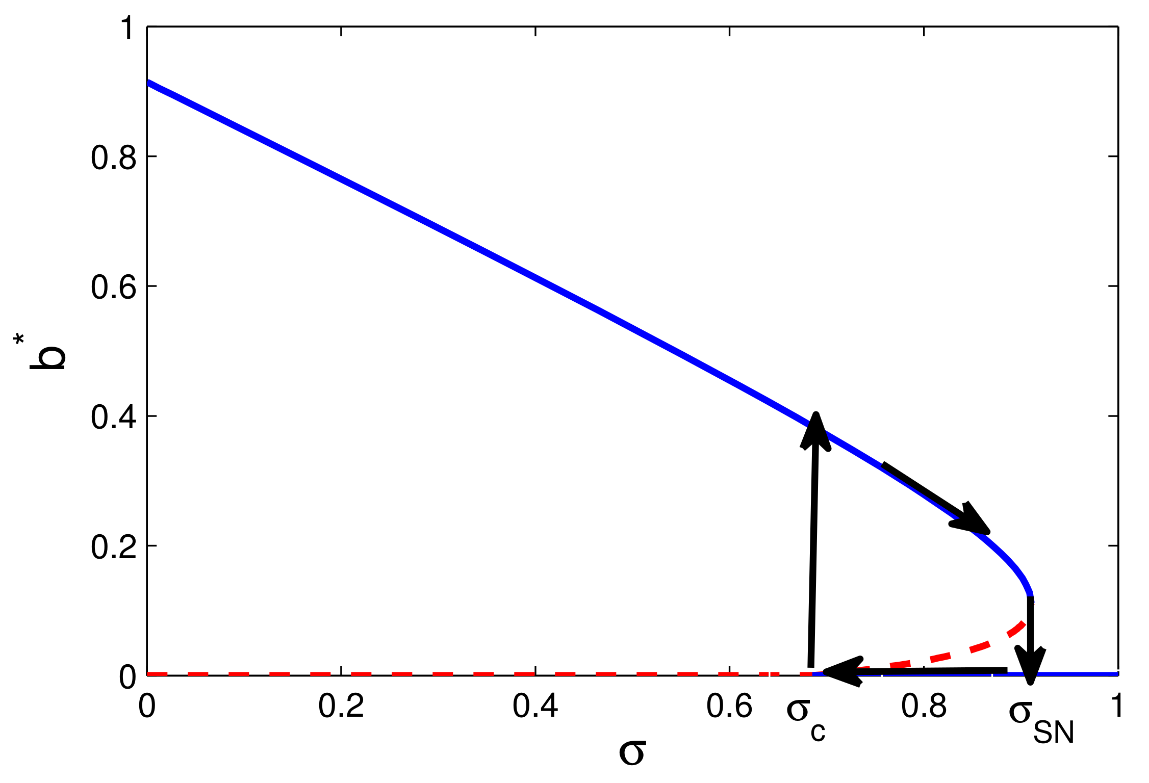
In this latter case, inducing a slight reduction of the dropout rate does not allow to restore the spreading of the campaign. To this aim, it is in fact necessary to drastically reduce below the value. This behavior is depicted in Figure 2 and clearly indicates a hysteretic phenomenology since the functioning and the current state of the system can be understood in a more detailed manner with reference to its past. In this sense, the effects on the dynamics persist after the causes that determined them have been removed.
As a consequence if the backward phenomenology can represent an opportunity, it nevertheless introduces a risk factor and, for this reason, it must be detected and adequately managed. This suggests the need for a more accurate characterization of the bistability range delimited by the transcritical threshold and by the saddle-node threshold . To this aim, we derive the analytical expression of the saddle-node bifurcation threshold . We first recall that the two campaign-standing equilibria and are such that:
where , and are defined in (6) and are the two positive solutions of the algebraic Equation (7) whose coefficients are defined in (8). More precisely,
with defined in (10) and the quantities and defined in (9). At , the two campaign-standing equilibria (unstable) and (stable) coalesce and disappear so that, for the campaign-free equilibria is the only attractor for the system. The saddle-node bifurcation of the two campaign-standing equilibria can be detected by requiring that so that . At this regard, it holds:
where
with defined in (14). By direct computation it easy follows that if then are real quantities and that, for , the inequalities hold. Therefore,
is the saddle-node bifurcation threshold and is the bistability range for model (5). In the next section, we show how these critical thresholds are affected by variations in the self-information level.
5. Effects of Self-Information on the Bifurcation Thresholds
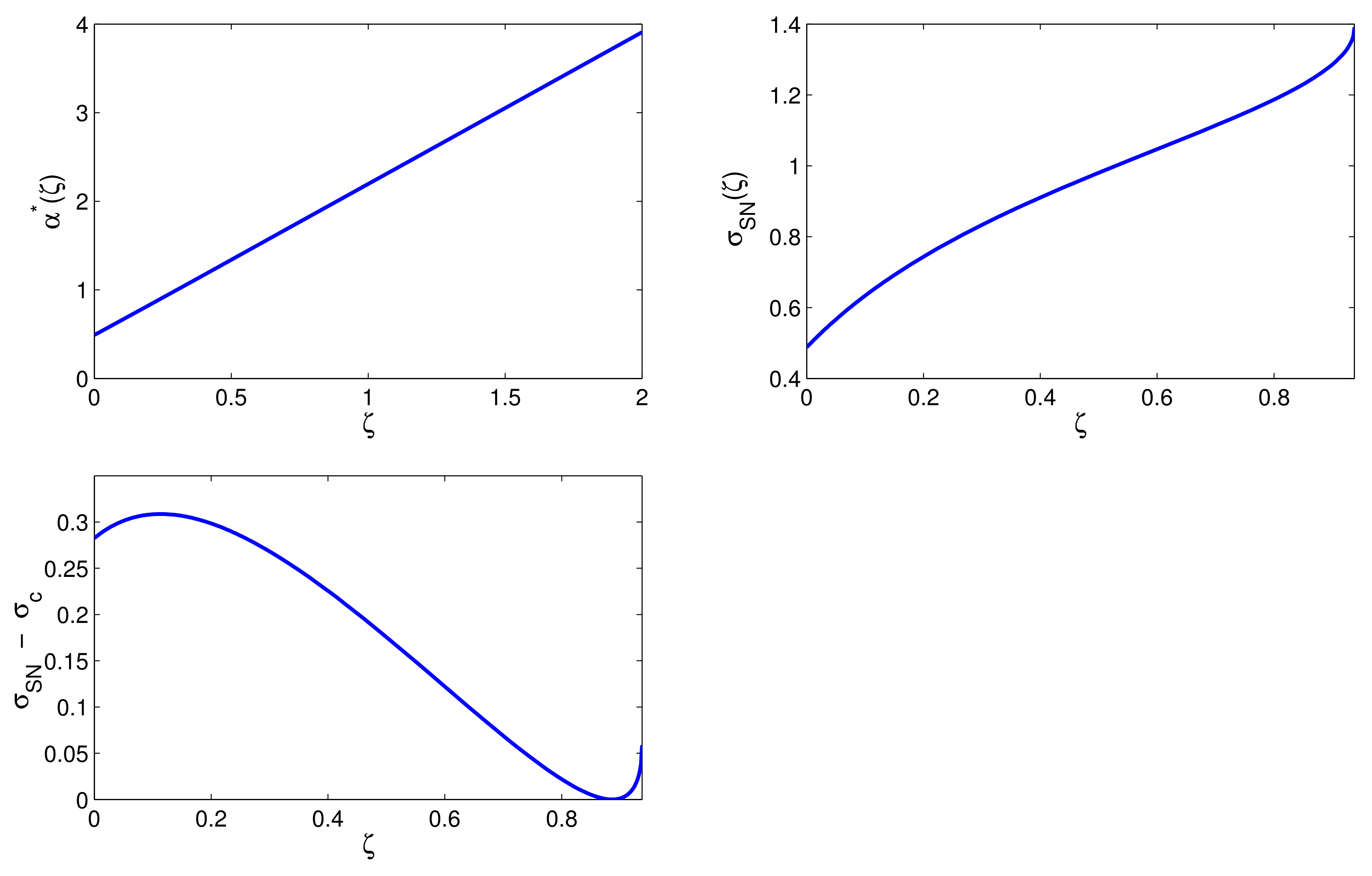
Since and k are the parameters specifically related to the self-information mechanism, we introduce the information parameter and consider the different bifurcation thresholds as function of , i.e.,
with as defined in (15). We observe that the saddle-node bifurcation threshold is a real quantity provided that the information variable is chosen in the range , where
Moreover, since in the backward scenario , the inequality
is always verified and is a positive quantity. We also observe that the transcritical bifurcation threshold is an increasing function of , being
Therefore an higher information increases the threshold , so that both in the forward and in the backward regime it becomes larger the range for which the campaign-standing equilibrium is the only attractor for the system.
Moreover, Figure 3 also indicates that:
- the threshold increases with increasing the information variable . This means that an higher information increases the threshold , favoring the forward regime with respect to the backward scenario. In this sense, information would act as a stabilizing mechanism;
- within the backward scenario, the saddle-node bifurcation threshold increases with increasing the information variable . This means that an higher information implies a higher value of in order to stop the campaign. However, the length of the bistability range does not have a monotone trend as function of the information variable . More precisely, for intermediate values of , the bistability range decreases whereas it increases when the values of are too small or too large. This would qualitatively mean that too much or too little information, although enlarging the chances of survival of the campaign, can have eventually a destabilizing effect on the system dynamics favoring sudden collapses in broadcasters that could lead to a sudden stop of the campaign according to a hysteretic phenomenology.
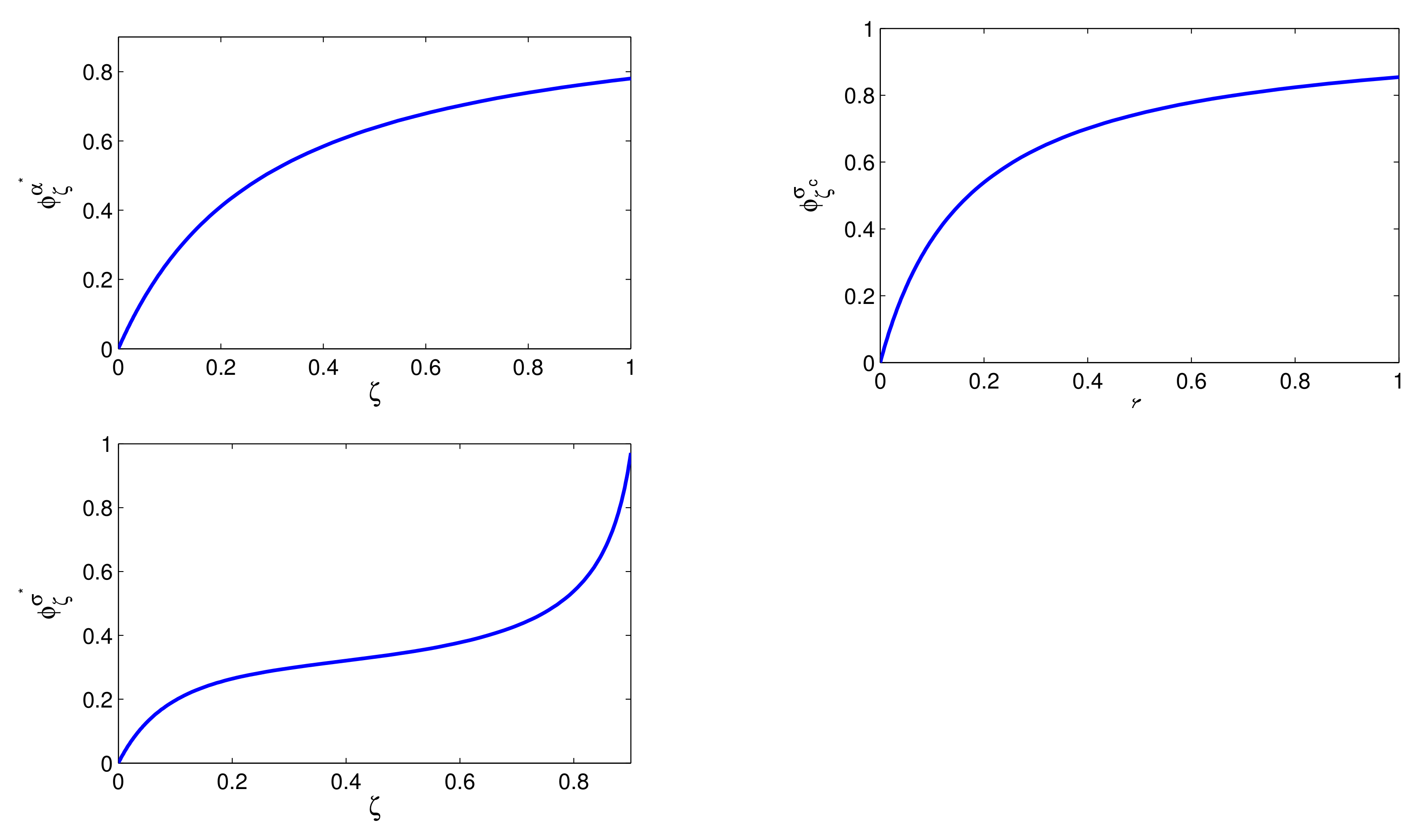
To give a more quantitative measure of the impact of the information parameter on the bifurcation thresholds (16), we will make use of the sensitivity analysis that is a useful tool to reveal how a certain parameter can influence the campaign transmission. The sensitivity of a certain variable with respect to system parameters can be measured through a sensitivity index that provides a quantitative measure of the relative change in a variable when a parameter changes. When the variable is a differentiable function of the parameter, the sensitivity index is defined as follows:
Definition 1.
[36] The normalized forward sensitivity index of a variable u, that depends differentiably on a parameter p, is defined as
The normalized forward sensitivity index of a variable with respect to a parameter is therefore the ratio of the relative change in the variable to the relative change in the parameter.
Figure 4 shows how the sensitivity index of the different thresholds , and varies with varying the information parameter . For both and , the sensitivity index is a saturating function of , the first increasing more slowly than the latter. The sensitivity of instead rapidly grows for enough low values and for enough high values of the information parameter ; on the contrary, it grows very slowly for intermediate values of . In Table 1, we show more quantitatively how variations in the information parameter can affect the different thresholds (16).
It is interesting to observe that affects such thresholds differently depending on the level of information we consider.
In the case of low information, is the most affected threshold: in fact, , which means that increasing (or decreasing) the parameter by , increases (or decreases) the transcritical threshold by . The less affected threshold is instead , being . However, for this case, the sensitivity indices for the three thresholds have numerical values fairly low and quite similar each others. A similar situation, but with higher values of the sensitivity indices is found for the case of intermediate levels of information for which the thresholds and are influenced by variations in the information parameter much more than the saddle-node bifurcation threshold . Also in this case, is the threshold most influenced by variations in the information parameter, being ; the less affected threshold is instead , since . The case of high levels of information presents a completely different scenario being now the most affected threshold with : this means that increasing (or decreasing) the parameter by , increases (or decreases) the saddle-node bifurcation threshold by . In this case, however, also the thresholds and are significantly influenced by variations in the information parameter .
These results seem to suggest that intermediate levels of information allow to spread the campaign in more controllable conditions. In fact, they seem to (i) favor a forward-type regime over a backward type, as it can be observed by the significant increase in the threshold; (ii) favor the presence of a single campaign-standing type attractor (significant increase in the threshold ) with respect to a bistability regime (loose impact on the threshold ). In this sense, intermediate levels of information are surely preferable to low ones. On the other hand, too high levels of information sensitively impact the saddle-node threshold, favoring a bistability situation where the chances of the campaign’s survival increase despite being exposed to the likely emergence of hysteretic dynamics.
The survival of the campaign obviously depends on the number of people who make it to spread and in the bistability range, when tends to , the level of broadcasters at the campaign-standing equilibrium tends to decrease, as it can be seen from the bifurcation diagram in Figure 1.
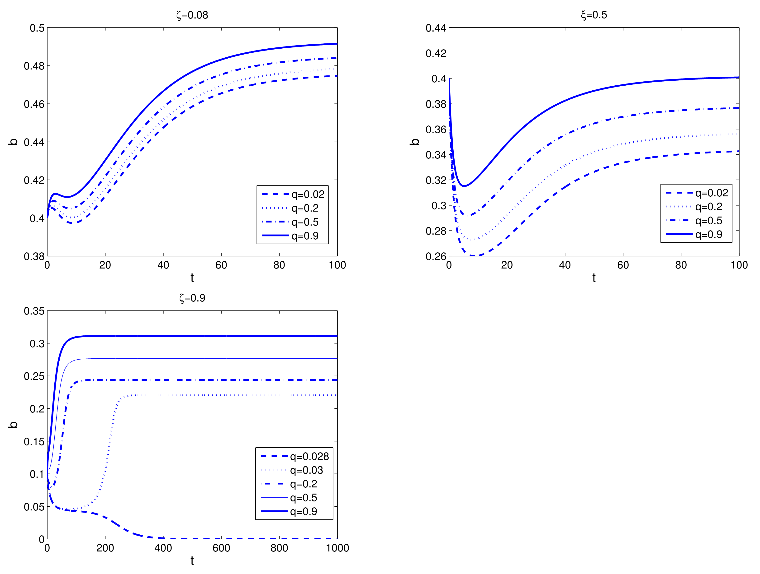
It is therefore interesting to ask whether the level of customer satisfaction linked to the self-information process can act as a destabilizing factor for the survival of the campaign. Numerical simulations in Figure 5 (Top) show that, for low or intermediate values of the self-information parameter , the campaign-standing equilibrium is rather resilient to variations in the level of the customer satisfaction q. However, increasing the level of self-information from low to intermediate, the impact of q also increases to the point that, for high values of , a threshold value can be found below which the referral campaign is driven to stop, Figure 5 (Bottom).
6. Conclusions
With this study we wanted to show that the concept of backward bifurcation, borrowed from epidemics, can be fruitfully exploited to shed light on the mechanism underlying the occurrence of hysteresis in marketing as well as for the strategic planning of adequate tools for its control.
In this paper, we considered a referral marketing model with self-information and evaluated how the interplay between a passive information (due to referrals) and an active information (due to self-information) impacts the sustainability of the viral campaign. We found that the emergence of a forward or a backward phenomenology is essentially linked to passive information mechanisms since the occurrence of these scenarios depends on the suitable interplay between the two parameters that regulate the reciprocal transition between the broadcaster and inert classes by the means of referrals.
Differently from epidemics, in the viral marketing context, a backward scenario could strengthen the campaign’s chances of survival. But if it can represent an opportunity from one side, on the other it introduces a risk factor because of the bistability range where system dynamics highly depends on the initial conditions. In this range hysteresis-type behaviors can hence emerge. Moreover, if in epidemics the main purpose is to ‘avoid’ a backward type scenario, for viral marketing this aim becomes learning to tame and eventually manage the backward phenomenology. In the present study, this has been shown to be the role of self-information that, however, needs to be properly calibrated. According to the Latin sentence ‘in medio stat virtus’, our analysis shows in fact that intermediate levels of self-information allow the campaign to spread in more controllable conditions by favoring the more reassuring forward-type regime over the backward one and, in both these cases, by widening the range of parameters in which the campaign-standing equilibrium is the only attractor for the system. Too high levels of information can instead broaden the region of parameters in which bistability occurs and, although enlarging the chances of survival of the campaign, can be responsible of sudden collapses in its spread. Just in this case, the level of customer satisfaction turns out to have a certain weight since a threshold customer satisfaction value can be found, below which, small fluctuations from the campaign-standing equilibrium value can lead the campaign to a sudden stop.
Therefore, even if hysteretic dynamics in referral campaigns may likely occur because intimately linked to the mechanism of referrals, an adequate level of self-information and a fairly high level of customer-satisfaction, can be two weapons capable to control hysteresis by transforming a potential risk into an opportunity.
In conclusion, this study represents a qualitative step to better understand how self-information can impact the sustainability of a referral marketing campaign and, within such a qualitative dimension, there is no presumption to fit the trend of a specific campaign. To provide further insight into the topic, two extensions are currently the subject of ongoing research: (i) giving the model a more quantitative dimension through a validation with a practical experience and (ii) exploring the possible impact of multilayer or multiplex networks, that may lead to some hidden patterns of influence and interplay between the self-information mechanism and the viral spreading of the campaign.
Funding
This research received no external funding.
Institutional Review Board Statement
Not applicable.
Informed Consent Statement
Not applicable.
Acknowledgments
The present work has been performed under the auspices of the Italian National Group for Mathematical Physics (GNFM-Indam). The author wishes to thank the anonymous Referees and the handling Editor for their valuable comments and remarks.
Conflicts of Interest
The author declares no conflict of interest.
References
- May, R.M. Uses and Abuses of Mathematics in Biology. Science 2004, 303, 790–793. [Google Scholar] [CrossRef] [PubMed] [Green Version]
- Volterra, V. Variazioni e fluttuazioni del numero di individui in specie animali conviventi. Mem. Acc. Lincei 1926, 2, 31–113. [Google Scholar]
- Lotka, A. Elements of Physical Biology; William and Wilkins: Baltimore, MD, USA, 1925. [Google Scholar]
- Sohn, K.; Gardner, J.; Weaver, J. Viral Marketing–More than a Buzzword. J. Appl. Bus. Econ. 2013, 14, 21–42. [Google Scholar]
- Kaplan, A.M.; Haenlein, M. Two hearts in three-quarter time: How to waltz the social media/viral marketing dance. Bus. Horizons 2011, 54, 253–263. [Google Scholar] [CrossRef]
- Reichstein, T.; Brusch, I. The decision-making process in viral marketing—A review and suggestions for further research. Psychol. Mark. 2019, 36, 1062–1081. [Google Scholar] [CrossRef] [Green Version]
- Bhattacharya, S.; Gaurav, K.; Ghosh, S. Viral marketing on social networks: An epidemiological perspective. Phys. A Stat. Mech. Appl. 2019, 525, 478–490. [Google Scholar] [CrossRef]
- Rodrigues, H.; Fonseca, M. Can information be spread as a virus? viral marketing as epidemiological model. Math. Methods Appl. Sci. 2016, 39, 4780–4786. [Google Scholar] [CrossRef] [Green Version]
- Ghosh, S.; Bhattacharya, S.; Gaurav, K.; Singh, Y. Going Viral: The Epidemiological Strategy of Referral Marketing. arXiv 2018, arXiv:1808.03780. [Google Scholar]
- Ghosh, S.; Gaurav, K.; Bhattacharya, S.; Singh, Y.N. Ensuring the Spread of Referral Marketing Campaigns: A Quantitative Treatment. Sci. Rep. 2020, 10, 11072. [Google Scholar]
- The Nielsen Company. Global Trust in Advertising. 2015. Available online: https://www.nielsen.com/wp-content/uploads/sites/3/2019/04/global-trust-in-advertising-report-sept-2015-1.pdf (accessed on 14 March 2021).
- Beretta, E.; Breda, D. Discrete or distributed delay? Effects on stability of population growth. Math. Biosci. Eng. 2016, 13, 19. [Google Scholar] [CrossRef]
- Buonomo, B.; d’Onofrio, A.; Lacitignola, D. Global stability of an SIR epidemic model with information dependent vaccination. Math. Biosci. 2008, 216, 9–16. [Google Scholar] [CrossRef] [PubMed]
- Feng, J.; Sevier, S.; Huang, B.; Jia, D.; Levine, H. Modeling delayed processes in biological systems. Phys. Rev. E. 2016, 94, 032408. [Google Scholar] [CrossRef] [Green Version]
- Rombouts, J.; Vandervelde, A.; Gelens, L. Delay models for the early embryonic cell cycle oscillator. PLoS ONE 2018, 13, e0194769. [Google Scholar] [CrossRef]
- Bischi, I.; Naimzada, A. A Kaleckian Macromodel with Memory. In Cycles, Growth and the Great Recession; Cristini, A., Leoni, R., Eds.; Routledge: London, UK, 2015. [Google Scholar]
- Matsumoto, A.; Chiarella, C.; Szidarovszky, F. Dynamic monopoly with bounded continuously distributed delay. Chaos Solitons Fractals 2013, 47, 66–72. [Google Scholar] [CrossRef]
- Krawiec, A.; Szydłowski, M. Economic growth cycles driven by investment delay. Econ. Model. 2017, 67, 175–183. [Google Scholar] [CrossRef]
- Sîrghi, N.; Neamtu, M.; Mircea, G.; Ramescu, D. The Deterministic Model With Time Delay for a New Product Diffusion in a Market. Timis. J. Econ. Bus. 2018, 11, 55–66. [Google Scholar] [CrossRef] [Green Version]
- Hughes, C.; Swaminathan, V.; Brooks, G. Driving Brand Engagement Through Online Social Influencers: An Empirical Investigation of Sponsored Blogging Campaigns. J. Mark. 2019, 83, 78–96. [Google Scholar] [CrossRef]
- Kryukov, E.; Malgin, V.; Malgina, I. The influence of Hysteresis in consumer’s behaviour for premium price evaluation. Manag. Mark. J. 2014, 12, 205–218. [Google Scholar]
- Hanssens, D. Keeps Working and Working and Working … The Long-Term Impact of Advertising. NIM Mark. Intell. Rev. 2015, 7, 42–47. [Google Scholar] [CrossRef] [Green Version]
- Moraru, A.; Barbulescu, A.; Duhnea, C. Consumption and hysteresis: The new, the old, and the challenge. Econ. Res. Ekon. Istraz. 2018, 31, 1965–1980. [Google Scholar] [CrossRef] [Green Version]
- Anguelov, R.; Garba, S.; Usaini, S. Backward bifurcation analysis of epidemiological model with partial immunity. Comput. Math. Appl. 2014, 68, 931–940. [Google Scholar] [CrossRef]
- Buonomo, B.; Lacitignola, D. On the backward bifurcation of a vaccination model with nonlinear incidence. Nonlinear Anal. Model. Control 2011, 16, 30–46. [Google Scholar] [CrossRef] [Green Version]
- Gumel, A. Causes of backward bifurcations in some epidemiological models. J. Math. Anal. Appl. 2012, 395, 355–365. [Google Scholar] [CrossRef] [Green Version]
- Lacitignola, D.; Saccomandi, G. Managing awareness can avoid hysteresis in disease spread: An application to Coronavirus Covid-19. Chaos Solitons Fractals 2021, 144, 110739. [Google Scholar] [CrossRef] [PubMed]
- Zhang, W.; Wahl, L.; Yu, P. Backward bifurcations, turning points and rich dynamics in simple disease models. J. Math. Biol. 2016, 73, 947–976. [Google Scholar] [CrossRef]
- Van den Driessche, P.; Watmough, J. A simple SIS epidemic model with a backward bifurcation. J. Math. Biol. 2000, 40, 525–540. [Google Scholar] [CrossRef] [PubMed]
- Smith, H. An Introduction to Delay Differential Equations with Applications to the Life Sciences; Springer Science & Business Media: Berlin/Heidelberg, Germany, 2010. [Google Scholar]
- Strogatz, S. Nonlinear Dynamics and Chaos: With Applications to Physics, Biology, Chemistry, and Engineering, 2nd ed.Studies in Nonlinearity; Westview Press: Nashville, TN, USA, 2014. [Google Scholar]
- Guo, D.; Zhang, Y. Neural Dynamics and Newton–Raphson Iteration for Nonlinear Optimization. J. Comput. Nonlinear Dyn. 2014, 9, 021016. [Google Scholar] [CrossRef]
- Lacitignola, D.; Diele, F. On the Z-type control of backward bifurcations in epidemic models. Math. Biosci. 2019, 315, 108215. [Google Scholar] [CrossRef] [PubMed]
- Lacitignola, D.; Diele, F. Using awareness to Z-control a SEIR model with overexposure. Insights on Covid-19 pandemic. Chaos Solitons Fractals 2021. under revision. [Google Scholar]
- Brauer, F. Backward bifurcations in simple vaccination models. J. Math. Anal. Appl. 2004, 298, 418–431. [Google Scholar] [CrossRef] [Green Version]
- Chitnis, N.; Hyman, J.; Cushing, J. Determining Important Parameters in the Spread of Malaria Through the Sensitivity Analysis of a Mathematical Model. Bull. Math. Biol. 2008, 70, 1272–1296. [Google Scholar] [CrossRef] [PubMed]
Figure 1.
Bifurcation diagram in the plane (). The other parameters are ; ; ; ; ; ; ; so that and . The solid lines (-) denote stability; the dashed lines (- -) denote instability. (Left) Forward scenario. The case , − At , system (5) exhibits a forward bifurcation. (Right) Backward scenario. The case , − At , system (5) exhibits a backward bifurcation. The value is the saddle-node bifurcation threshold.

Figure 2.
Graphical representation of an hysteresis cycle on the bifurcation diagram in the plane () in the case , where a backward scenario is obtained. The other parameters are as in Figure 1 (right). Here , and the value is the saddle-node bifurcation threshold. The solid lines (-) denote stability; the dashed lines (- -) denote instability.

Figure 3.
Thresholds (16) as function of the information variable . The other parameters are chosen as in Figure 1. (Top-left) The threshold as function of . (Top-right) The saddle-node bifurcation threshold as function of . The threshold is feasible in the range , with (Bottom) The length of the bistability range, i.e., , within the backward scenario as function of . The bistability range is increasing for and and it decreases for . Here ; ; .

Figure 4.
Sensitivity indices of the different thresholds , and as function of the information variable . The other parameters are chosen as in Figure 1. (Top-left) Plot of the sensitivity versus the information variable ; (Top-right) Plot of the sensitivity versus the information variable ; (Bottom) Plot of the sensitivity versus the information variable .

Figure 5.
Impact of the customer satisfaction parameter q on the referral campaign in the bistability region, , for different levels of self-information. Initial conditions are chosen in the neighbouring of the campaign-standing equilibrium. The other parameters are as in Figure 1. (Top-left) Low level of the self-information parameter, i.e., () and . (Top-right) Intermediate level of the self-information parameter, i.e., () and . (Bottom) High level of the self-information parameter, i.e., () and .


Table 1.
Sensitivity indices of the thresholds , and for three different levels of information: low, intermediate and high. The numerical values of the system parameters used for the computations are: ; ; ; ; . Here ; ; .
Table 1.
Sensitivity indices of the thresholds , and for three different levels of information: low, intermediate and high. The numerical values of the system parameters used for the computations are: ; ; ; ; . Here ; ; .
| Low Information | Intermediate Information | High Information |
|---|---|---|
Publisher’s Note: MDPI stays neutral with regard to jurisdictional claims in published maps and institutional affiliations. |
© 2021 by the author. Licensee MDPI, Basel, Switzerland. This article is an open access article distributed under the terms and conditions of the Creative Commons Attribution (CC BY) license (http://creativecommons.org/licenses/by/4.0/).
Share and Cite
MDPI and ACS Style
Lacitignola, D. Handling Hysteresis in a Referral Marketing Campaign with Self-Information. Hints from Epidemics. Mathematics 2021, 9, 680. https://doi.org/10.3390/math9060680
AMA Style
Lacitignola D. Handling Hysteresis in a Referral Marketing Campaign with Self-Information. Hints from Epidemics. Mathematics. 2021; 9(6):680. https://doi.org/10.3390/math9060680
Chicago/Turabian StyleLacitignola, Deborah. 2021. "Handling Hysteresis in a Referral Marketing Campaign with Self-Information. Hints from Epidemics" Mathematics 9, no. 6: 680. https://doi.org/10.3390/math9060680
Note that from the first issue of 2016, this journal uses article numbers instead of page numbers. See further details here.