
Black-Box-Based Mathematical Modelling of Machine Intelligence Measuring


Department of Electrical Engineering and Information Technology, Faculty of Engineering and Information Technology, “George Emil Palade” University of Medicine, Pharmacy, Sciences, and Technology of Tg. Mures, Gh. Marinescu 38, 540142 Tg. Mures, Romania
Mathematics 2021, 9(6), 681; https://doi.org/10.3390/math9060681
Submission received: 11 December 2020
/
Revised: 14 March 2021
/
Accepted: 18 March 2021
/
Published: 22 March 2021
(This article belongs to the Section Mathematics and Computer Science)
Abstract
:Current machine intelligence metrics rely on a different philosophy, hindering their effective comparison. There is no standardization of what is machine intelligence and what should be measured to quantify it. In this study, we investigate the measurement of intelligence from the viewpoint of real-life difficult-problem-solving abilities, and we highlight the importance of being able to make accurate and robust comparisons between multiple cooperative multiagent systems (CMASs) using a novel metric. A recent metric presented in the scientific literature, called MetrIntPair, is capable of comparing the intelligence of only two CMASs at an application. In this paper, we propose a generalization of that metric called MetrIntPairII. MetrIntPairII is based on pairwise problem-solving intelligence comparisons (for the same problem, the problem-solving intelligence of the studied CMASs is evaluated experimentally in pairs). The pairwise intelligence comparison is proposed to decrease the necessary number of experimental intelligence measurements. MetrIntPairII has the same properties as MetrIntPair, with the main advantage that it can be applied to any number of CMASs conserving the accuracy of the comparison, while it exhibits enhanced robustness. An important property of the proposed metric is the universality, as it can be applied as a black-box method to intelligent agent-based systems (IABSs) generally, not depending on the aspect of IABS architecture. To demonstrate the effectiveness of the MetrIntPairII metric, we provide a representative experimental study, comparing the intelligence of several CMASs composed of agents specialized in solving an NP-hard problem.
1. Introduction
Computer systems encounter various issues during problem-solving, including high computational complexity, especially in the case of NP-hard problems, and the presence of different types of uncertainties, e.g., due to missing or erroneous data. Usually, computationally complex problems can be effectively solved by intelligent agent-based systems (IABSs), ranging from individual agents (IAGs) to cooperative multiagent systems (CMASs).
There are diverse CMASs specialized in difficult-problem-solving that are considered intelligent [1,2,3,4]. Applications of agent-based systems (ABSs) include the following: diverse problems solving in Industry 4.0 [5]; adaptive clustering [6]; modeling strategic interactions in diverse democratic systems [7]; investigation on supply chain of product recycling [8]; detecting the proportion of traders in the stock market [9]; control design in the presence of actuator saturation [10]; agent-based simulator for environmental land change [11]; distributed intrusion detection [12]; investigations of complex information systems [13]; discovering Semantic Web services through process similarity matching [14]; power system control and protection [15]; studies on task type and critic information in credit assignments [16]; planning with joint actions [17]; patient scheduling [18]; study compliance with safety regulations [19]; multi-objective optimization [20]. Studies present applications of computational intelligence in domains including the [21] industry and environment. Problem-solving based on computational intelligence techniques include adaptive reflection detection and location in iris biometric images [22], arithmetic codes for concurrent error detection in artificial neural networks [23], and support in medical decision-making [24,25].
This paper defines ICMASs formed of agent members that are not necessarily intelligent, but at the level of the whole system, a measurable increase in collective intelligence emerges [1,2]. Machine intelligence measures are considered in the context of difficult-problem-solving abilities. Diverse studies and research related to the performance and intelligence measures in the paper [26] are presented. The problem-solving ability of interest should be established by a human assessor (Ha) who would like to make the problem-solving intelligence measurement. Higher intelligence means a measurably improved problem-solving ability. The intelligent biological life forms have variability in intelligence. For problem-solving, a CMAS can manifest higher or lower intelligence, exhibiting variability. For the solution of a difficult problem, a CMAS could manifest sometimes a statistically high or low extreme (outlier) intelligence metric value. According to our bibliographic study, the most important properties of intelligence metrics should include universality, accuracy, and robustness [27,28].
The MetrIntPair metric [27] can make an accurate comparison of the intelligence of two CMASs. It takes into account all the aforementioned considerations. Intelligence measurements were also considered in the context of difficult-problem-solving abilities. This metric can also be used to make classifications of the considered CMASs based on their intelligence, where two CMASs with the same (from a statistical point of view) intelligence can be included in the same class. MetrIntPair can make a differentiation in intelligence between two CMASs even if the numerical difference between the measured intelligence is small. In the framework of intelligence comparisons using the MetrIntPair metric, a statistical analysis is performed. In the case of comparing more than two CMAS intelligence, one idea is to use MetrIntPair in pair-by-pair comparisons of the CMASs. Unfortunately, this increases the chance for a statistical intelligence comparison error, known as the Family-wise error rate (FWER). A more detailed analysis of this subject and the calculus of the FWER value [29] are presented in the discussion section. This is a motivation for the design of a more general metric that could analyze simultaneously the intelligence of any number of systems and classify them based on their problem-solving intelligence in intelligence classes.
In this paper, a novel mathematically grounded metric called Pairwise Machine Intelligence Measuring and Comparison of Multiple Intelligent Systems (MetrIntPairII) is proposed. It is able to make an accurate and robust comparison of a large number of CMASs. It conforms to all the aforementioned considerations. MetrIntPairII represents a generalization and an extension of the MetrIntPair metric, conserving all of its properties. The generalization consists in the fact that MetrIntPairII is not restricted to the application on two CMASs. The extension consists in the fact that it can handle intelligence indicator data that does not satisfy the assumption of normality. Furthermore, an advantage of MetrIntPairII over MetrIntPair in the context of intelligence comparisons is that it does not produce an FWER error. To prove the effectiveness of the MetrIntPairII metric, we investigate a case study, using different CMASs that operate by mimicking diverse biological swarms. In this context, the intelligence of a few CMASs specialized in solving a type of NP-hard problem are measured and compared.
The rest of this paper is organized as follows: Section 2 reviews state-of-the-art metrics for intelligence measurement. In Section 3, the MetrIntPairII metric is presented, together with the notions that stand at its foundation. Section 4 presents the performed experimental study, which demonstrates the effectiveness of the MetrIntPairII metric. In Section 5, various aspects related to the considered metric are discussed. In the last section, the conclusions of this research are summarized.
2. Metrics for Measuring Machine Intelligence
Many of the IABSs are CMASs. Even in very simple CMASs, an increased intelligence can emerge at the system’s level. For instance, Yang et al. [1] proposed an ICMAS composed of simple reactive mobile agents that are able to mimic the behavior of a human network administrator.
One of the earliest famous definitions of machine intelligence was presented by Alan Turing [30] in 1950. A computing system was considered intelligent if a human assessor could not decide the nature of the system as being human or artificial based on questions asked from a hidden room. The definition is based on the idea of an artificial cognitive system that is able to mimic the cognition of a human being.
As examples of systems that could best fit the Turing’s criteria of intelligence appreciation, from a specialty knowledge point of view, similar to the knowledge that human specialists have, the expert systems (ESs) can be mentioned. ESs can solve specialty problems, similarly to human specialists, and have a diversity of applications [31].
Several studies have been performed related to machine intelligence, human intelligence, and the analogies and differences between them, analyzing different aspects of Turing’s test proposal. A relatively recent study on Turing’s test was presented by Sterret [32], analyzing how Watson, an IBM-developed question-answering computer, could compete against humans in the Jeopardy game. There is also the famous competition between the chess playing machine named Deep Blue and the chess grandmaster Kasparov [33]. Besold et al. [34] studied diverse difficult problems for humans that could be used as benchmark problems for IABSs. Detterman [35] proposed an interesting challenge regarding the Machine Intelligence Quotient (MIQ) measured by well-known IQ tests developed for humans. Sanghi and Dowe [36] presented an intelligent computer program that was evaluated successfully on some standard human IQ tests. According to the authors, it surpassed the average human intelligence (by 100) on some tests [36]. Even in this successful situation from the side of the computing system, we consider that artificial and human intelligence cannot be directly compared at the general level.
MetrIntSimil [37] represents an accurate and robust metric that can be applied for a comparison of similarity in intelligence of any number of cooperative multiagent systems.
An interesting study realized at the US National Institute of Standards and Technology was presented by Schreiner [38], aiming to create standard measures for intelligent systems (ISs). Schreiner studied the research question of how precisely ISs are defined, and analyzed how to measure and compare the intelligence capabilities of ISs. Park et al. [39] introduced the notion of an intelligence task graph to study the measurement of machine intelligence of human–machine cooperative systems. Anthon and Jannett [40] analyzed the ABS intelligence considering the ability to compare alternatives with different levels of complexity. In their research, an agent-based distributed sensor network system was considered. The proposal was tested by comparing MIQs in diverse scenarios. Hernández-Orallo and Dowe [41] proposed a general test called the universal anytime intelligence test. That study considered that such a test should be able to measure the intelligence level, which could be very low or very high in diverse situations. The presented approach was based on the C-tests and compression-enhanced Turing tests developed in the late 1990s. Different tests were discussed, highlighting their limitations, and some new ideas were introduced and need to be studied for the development of a universal intelligence test.
ExtrIntDetect [42] represents a universal method that can be applied for the identification of intelligent cooperative multiagent systems with extreme intelligence.
Legg and Hutter defined an intelligence measure [43], presuming that the performance in easy environments counts less toward an agent’s intelligence than does the performance in difficult environments. Hibbard [44] proposed a metric for intelligence measurement based on a hierarchy of sets of increasingly difficult environments. Hibbard considers an agent’s intelligence measurement according to diverse considerations related to difficult-problem-solving ability.
In [28], a novel metric called MetrIntComp for the comparison of two CMASs’ intelligence was proposed. Intelligence measuring was considered based on the principle of difficult-problem-solving abilities. MetrIntComp is able to make a differentiation in intelligence between the two CMASs even if the numerical difference between the measured intelligence values is low. MetrIntComp makes also a classification of the considered CMASs based on their intelligence. According to this classification, two CMASs with the same intelligence (from a statistical point of view) can be included in the same class.
Liu et al. [45] present a recent complex study regarding the analysis of the intelligence quotient and the grade of artificial intelligence.
In [46], a metric that is able to compare the intelligence of a system with a reference intelligence is presented. The designed metric is also able to measure the evolution in intelligence of swarm systems.
In [47], a novel universal metric called MeasApplInt able to measure and compare the real-life problem solving machine intelligence of two cooperative multiagent systems systems at an application is proposed. The studied intelligent systems are classified in intelligence classes. Systems classified in the same class can solve problems at the same level of intelligence.
Usually, intelligence is required when the problems to be solved are characterized by different kinds of difficulties. In this sense, the main purpose of endowing systems with intelligence is to obtain improvements in solving difficult problems. Machine intelligence must be considered based on difficult-problem-solving abilities. Measuring machine intelligence is important to develop highly intelligent problem-solving approaches. At the same time, it should enable the selection of the most appropriate systems, based on their intelligence.
Each of the metrics/methods presented in the scientific literature is based on some specific ideology of intelligence measuring. Based on this fact, most of them cannot be compared. There is no standardization of intelligence measuring, nor is there a universal vision on what an intelligence’s metric should measure. One type of difficult problem could be solved by IABSs with a large diversity of architectures whose intelligence must be measured. This motivates the necessity to design universal metrics. One of the main drawbacks of actual metrics is their limitation in universality.
3. The Proposed MetrIntPairII Metric
In the following, we present a novel metric called Pairwise Machine Intelligence Measuring and Comparison of Multiple Intelligent Systems (MetrIntPairII). The metric is described in the form of an algorithm abbreviated as MetrIntPairII.
3.1. Description of the Proposed MetrIntPairII Metric
This subsection introduces the notion intelligence indicator of solving difficult problems. An intelligence indicator is established by an Ha in order to obtain a quantitative measure of the type of problem-solving intelligence that represents interest.
The following notations are used: Coop = {Coop, Coop, …, Coop} denotes the set of CMASs to be compared; |Coop| = m represents the cardinality (number) of compared CMASs; Int = {Int, Int, …, Int}; Int = {In1, In1, …, In1}, Int = {In2, In2, …, In2}, …, Int = {Inm, Inm, .., Inm} denote the obtained intelligence indicators as a result of intelligence measurements using a set of test problems Probl = {Prl, Prl, …, Prl}. Int represents the intelligence indicators for Coop; … Int represents the intelligence indicators for Coop. Table 1 presents the structuring of the measured intelligence indicator data. A line from Table 1, for instance, Prl, In1, In2, …, Inm, represents the measured Prl problem-solving intelligence measure for CoopCoop, …, Coop. In1 represents the Prl problem-solving intelligence measure for Coop … Inm represents the Prl problem-solving intelligence measure for Coop. The number of problems used with the purpose of intelligence measurements is represented by |Probl| = k; |Int| = |Int| = … = |Int| = k represents the cardinality of Int, Int, …, Int.
The number of problems used with the purpose of intelligence measurements is represented by |Probl| = k; |Int| = |Int| = … = |Int| = k represents the cardinality of Int, Int, …, Int.
A problem-solving intelligence measure is expressed as an intelligence indicator value. Based on the intelligence indicator values of a CMAS, what we call the Machine Intelligence Quotient (MIQ) can be obtained. This is an indicator of the central intelligence tendency. The sequence MIQ, MIQ, …, MIQ denotes the machine intelligence quotients of the Coop, Coop, …, Coop obtained by the measurement of the problem-solving intelligence using the set of test problems Probl. The MIQ of the Coop, Coop, …, Coop calculus is considered as the mean or the median of Int, Int, …, Int. It is calculated as the mean in the parametric case when all the intelligence indicator data Int, Int, …, Int pass the normality assumption. It is calculated as the median in the nonparametric case when not all the intelligence indicator data Int, Int, …, Int pass the normality assumption.
It must be noted that different sets of experimental intelligence evaluations could give slightly different MIQ values. This phenomenon is similar to the case of human intelligence tests, where a human obtains an evaluation result of his/her Intelligence Quotient (IQ), but at another evaluation, a slightly different IQ could be obtained. The proposed metric takes into consideration this aspect, which is called variability in intelligence. The central intelligence tendency of an ICMAS is described by the MIQ value and some additional indicators that include the mean, the standard deviation (SD), the confidence level of the mean (CL) (the use of 95% CL is recommended in most cases, and even other values such as 90% or 99% can be used), the lower confidence interval of the mean (LCI) and the upper confidence interval of the mean (UCI), both of which are calculated at an established CL level, and the coefficient of variation (CV) defined as CV = 100 × (SD/mean), expressed as a percentage to be easier to interpret by an Ha. The previously introduced indicators enable a statistical characterization of intelligence that allows for the formulation of diverse conclusions. For instance, CV is used as an indicator of the homogeneity–heterogeneity, and homogeneous intelligence means that there is not much significant variation in the problem-solving intelligence.
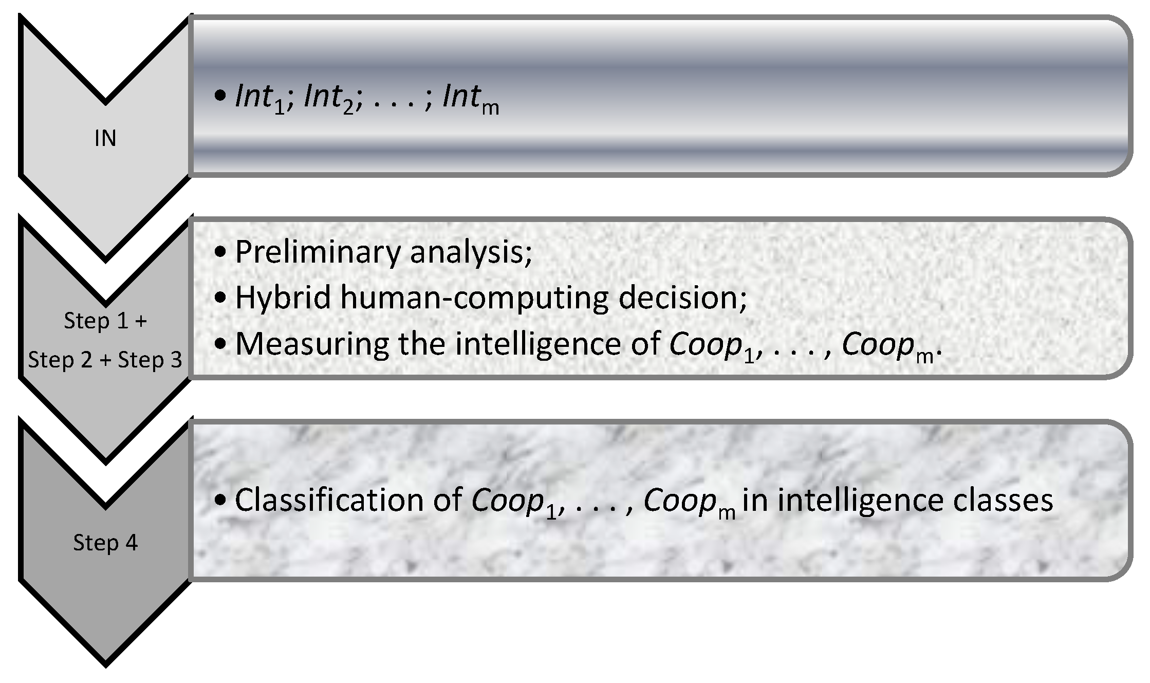
The MetrIntPairII algorithm compares the intelligence of Coop on the Probl testing problems set. It verifies whether the intelligence of Coop, Coop, …, Coop is statistically equal and makes a classification of the studied CMASs in intelligence classes. In the following, the null hypothesis, denoted as H, is the statement that the intelligence of Coop,Coop, …, Coop is equal from a statistical point of view (the difference is not statistically significant), meaning that all the analyzed CMASs should be included in the same intelligence class. H is denoted as the alternative hypothesis, which indicates that the intelligence of Coop, Coop, …, Coop are not all equal from a statistical point of view, and there is a difference in intelligence between at least two of them. It can be concluded that all analyzed CMASs cannot be included in the same class. MetrIntPairII uses as input Int, Int, …, Int. The “@” symbol specifies that the performance of a specific set of processing’s. For example, “@Apply the Friedman test with the More significance level.” specifies that the Friedman test is applied, as presented in the scientific literature, with the More significance level. Figure 1 briefly presents the main processing steps performed by the MetrIntPairII: Intelligence Comparison Algorithm.
A dataset is called homogeneous if CV < C, relatively homogeneous if CV∈ [C, C), relatively heterogeneous if CV∈ [C, C), and heterogeneous if CV ≥ C. Recommended values include C = 10, C = 20, and C = 30, as usually they are the most appropriate.
Some studies [48,49] compare the most frequently used tests for verification of the normality assumption, such as the One-Sample Kolmogorov–Smirnov test(KS test), the Shapiro–Wilk test(SW test), and the Lilliefors test(Lill test). The Lill test is an adaptation of the KS test. The SW test was proved to have the most statistical power for significance from the studied tests. It was noted in [48,49] that powerful normality tests could have disadvantages that must also be considered in decisions. For instance, in the case of the SW test, it was proved that it does not work well with many identical values.
| Algorithm 1. MetrIntPairII: Intelligence Comparison Algorithm |
| INPUT:Int;Int;…; Int; OUTPUT:MIQ; MIQ;…;MIQ; DecInt; Decision on classification. Step 1. Preliminary analysis. @Establish CL;@Makes a statistical analysis for Int, Int, …, Int by obtaining the: mean; LCI; UCI; minimum; maximum; median; SD; variance; CV; @Analyze the homogeneity/heterogeneity of Int, Int, …, Int based on the CV values. @Verify if Int, Int, …, Int pass the normality assumption. Step 2. Hybrid human-computing system decision. @Based on the Int, Int, …, Int data homogeneity/heterogeneity and normality ask Ha whether he/she decides for the application of an extreme detection test or the application of a data transformation. @Set the PreProcessing decision. If (PreProcessing="YesOutl”) Then @Apply an outlier detection test; ElseIf (PreProcessing="YesTransf”) @Apply a transformation to intelligence indicators data. EndIf Step 3. Measuring the intelligence ofCoop, …, Coop. Normality verification ofInt, Int, …, Int. If(IntandInt … and Int are normally distributed) Then Passed:="Yes”; ElsePassed:="No”; EndIf @Choose the significance level αMore. Calculate the MIQs as the mean or the median. @Calculate MIQ,MIQ, …, MIQ. Step 4. Classification based on the intelligence measurement. If (Passed="Yes") Then @Apply the Repeated Measure Anova with αMore. @Obtain p-value. Else @Apply the Friedman test with αMore. @Obtain the p-value. EndIf If (p-value>More) Then@Accept H. DecInt:="Coop,Coop, …, Coop intelligences are equal”; ElseIf((Passed= "Yes”) and (p-value<More)) Then @Apply the Tukey–Kramer Multiple Comparisons test. @Establish the decision on the classification ofCoop, Coop, …, Coop based on their intelligence. ElsePassed="No” and p-value <More. @Apply the Dunn test. @Make the decision on the classification of Coop,Coop, …, Coop based on their intelligence. EndIf EndMetrIntPairIIAlgorithm |
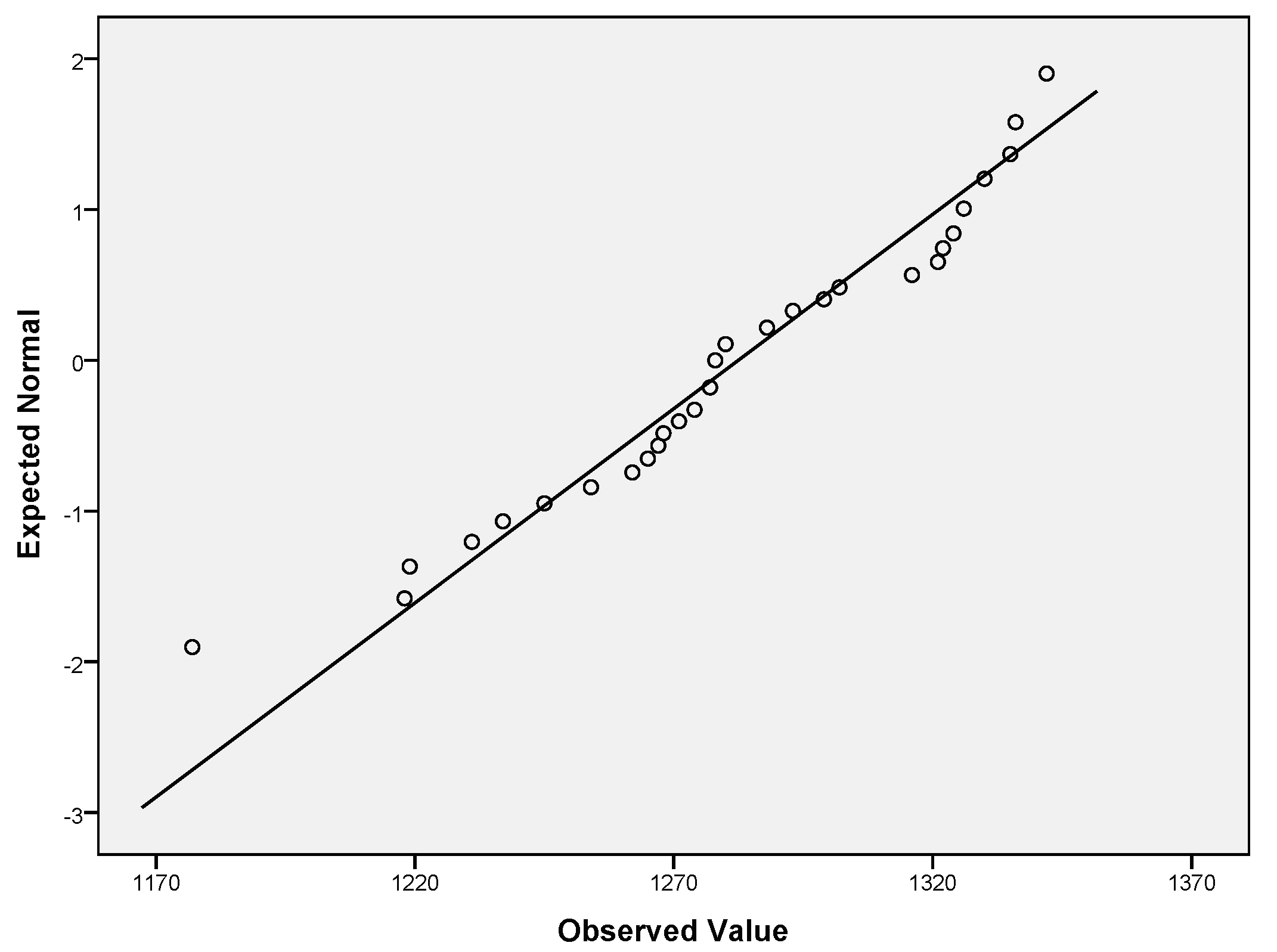
In our algorithm, for the normality verification, we have chosen the KS test [50,51,52], the Lill test [51,52,53], and the SW test [54]. The Quantile-Quantile plot (QQ plot) is a scatterplot appropriate for the normality visual appreciation. From an interpretation point of view, a QQ plot is a plotted reference line. In the case of normally distributed data, the points should fall approximately along this reference line. The greater the departure from the reference line, the greater the evidence is for the conclusion that the data fail the normality assumption. The joint use of the QQ plot with the SW test is suggested for accurate verification of the normality assumption.
In usual applications, it is sufficient to use the SW test jointly with the QQ plot. The SW test is appropriate even in the case of a normality evaluation of smaller sets of data.
Step 2 of the algorithm includes a hybrid human–computing system decision. This is based on the consideration that a human has some problem and domain-specific knowledge that can help him/her in more efficient decisions in some situations than computing systems. This step in some situations could be implemented as an automatic decision.
In the nonparametric case (the samples of at least one of the intelligence indicators are not normally distributed), to obtain normally distributed data, an Ha could decide for the elimination of extreme (outlier) intelligence indicator values. An intelligence indicator sample could contain extreme intelligence values. It is called the extreme intelligence indicator value, a very high or very low intelligence value, statistically significantly different from other intelligence indicator values. For the detection of extreme values, we used a statistical method called the Grubbs test for outlier detection, also called the ESD method (extreme studentized deviate) [55,56,57,58]. The assumption of the Grubbs test is the expected normality. The dataset can be reasonably approximated by a normal distribution. This must be first verified or known before its application. It is proposed that the Grubbs test be used with the significance level αGrubbs = 0.05, and other values can be considered, such as 0.01 or 0.1. At first application, the Grubbs test can identify a single extreme if there are any. If an extreme value is detected, then it is the statistically significantly most different value from those other measured intelligence indicator values. If an extreme is detected, one may consider applying the extreme detection test again. It can be applied recursively several times until no further extremes are identified.
Whenever the Grubbs test detects an extreme intelligence indicator in an intelligence indicator dataset, this value is removed together with the corresponding paired values from the other intelligence indicators datasets. For instance, in the case of the problem denoted Prl, the corresponding intelligence indicator value In1 (from In) is identified as an extreme, and In2, …, Inm are then also removed from the samples In, …, In.
Alternately, if the sample intelligence data does not pass the normality assumption, a transformation can be applied to obtain normally distributed data. Some of the most commonly used normalizing transformations, are indicated in Table 2 [59]. IN denotes an arbitrary dataset.
At Step 1 of the algorithm, statistical analysis is performed, and the results are used to make intermediary decisions on the intelligence indicator data and to decide on further processing steps. It is also appropriate to make some additional characterizations of the intelligence variability of the studied CMASs.
Step 4 of the algorithm performs the classification of the studied CMASs based on their intelligence. For effective comparison of the intelligence of the CMASs, the Repeated Measure Anova test [60,61] is used in the parametric case, when Int, Int, … Int pass the normality assumption. In the nonparametric case, when not all of Int, Int, … Int are normally distributed, the Friedman Two-Way Analysis of Variance by Ranks test (the Friedman test) is used [62,63]. When using the Friedman test, it is important to use a sample size of at least 12 in order to obtain an accurate p-value. In choosing each of the tests, the αMore significance levels value should be established. It is suggested that a value of αMore = 0.05 be used (other values such as 0.01 and 0.1 can also be used), which is frequently the most appropriate. αMore denotes the probability of making a type I error, signifying the rejection of H when it is true. As a motivation for choosing this significance level value, it must be mentioned that the smaller the significance level is, the less likely it is to make a type I error, and the more likely it is to make a type II error.
In the proposed MetrIntPairII metric algorithm, a p-value > αMore implies that H can be accepted at the established significance level. In this case, it can be concluded that, even if there is a numerical difference between the calculated MIQ, MIQ, …, MIQ values, there is no statistical difference in the intelligence of the studied CMASs. The numerical difference is the result of the variability in the intelligence of the CMASs. From a classification point of view, Coop, Coop, …, Coop can be classified in the same class of intelligence, in the sense that they can solve the considered class of problems with the same level of intelligence.
If H is accepted, then it can be concluded that the intelligence level of MIQ, MIQ, …, MIQ is statistically significantly different (there is a significant difference between at least two of them). Accordingly, from the point of view of classification, Coop, Coop, …, Coop cannot be classified in the same intelligence class. To distribute Coop, Coop, …, Coop into intelligence classes, the following post-tests are used: the Tukey–Kramer Multiple Comparisons test [64,65] (in the parametric case, when all the samples from Int pass the normality assumption) and the Dunn test [66,67] (in the non-parametric case, when not all the samples from Int pass the normality assumption). Additional explanations related to how the classification is accomplished based on the Tukey–Kramer post-test and the Dunn post-test are provided at the end of the experimental study presented in the next section. It is recommended that the application of both tests be at the significance level 0.05, and other significance levels such as 0.01 and 0.1 can be applied as well.
Dunn’s test compares the difference in the sum of ranks between two intelligence indicator sets with the expected average difference. For each pair of intelligence indicators, the p-value is obtained.
The Tukey–Kramer post-test is a single-step multiple-comparison statistical test. It can be used separately or in conjunction with, as a post-hoc of ANOVA, to find means that are significantly different from each other. It compares all possible pairs of means and is based on a studentized range distribution.
3.2. Intelligence Indicator Calculus Based on More Intelligence Components Values
Choosing the most appropriate intelligence indicator is the responsibility of the Ha who wishes to measure the intelligence and to compare the problem-solving intelligence of two or more CMASs. He/she could choose the most preferable one based on what he/she indicates as problem-solving intelligence, with respect to the type of intelligence that he/she would like to measure.
3.2.1. An Illustrative Example for the Notion: Type of Intelligence
The scenario of an intelligent transporting agent being able to autonomously pilot a car with a passenger.
In the considered Travelling Salesman (TSP) type of problem, a passenger starting from a city located in a country with a certain number of cities would like to visit with the help of a transporting agent each city once and return to the starting city with the smallest cost. Some examples of intelligence types that the pilot agent could use are enumerated below:
- 1.
- Type: Communication intelligence. The capacity to communicate with the passenger from the car. This may be implemented to work via voice commands.
- 2.
- Type: Intelligence in avoiding static objects that might appear on the road.
- 3.
- Type: Intelligence in avoiding collisions with other cars.
- 4.
- Type: Intelligence in avoiding humans who cross the road irregularly.
- 5.
- Type: Intelligence in avoiding animals that cross the road irregularly.
- 6.
- Type: Intelligence in planning efficient routes.
In this scenario, the Ha should establish the type of intelligence that he/she would like to measure at a specific moment of time. The Ha can choose, for instance, Type, which could be measured as the percentage of correctly recognized voice commands and the accuracy of their execution. Type could be measured, for instance, based on the aspect of how close the obtained route is to the shortest possible route.
A pilot agent AG may be more intelligent based on a specific type of intelligence than another pilot agent AG, while for another type of intelligence, the situation could be vice versa. For instance, AG could be more intelligent than AG in avoiding humans that cross the road, while AG could be more intelligent than AG in communication with the passenger.
If necessary, the intelligence indicator value can be calculated as the weighted sum of some components that characterize different aspects of the CMAS’s intelligence, using the formula:
where z represents the number of considered components; mes, mes, …, mes represent the considered components at a specific problem-solving intelligence evaluation; wgh, wgh, …, wgh represent the weights/importance of the components.
3.2.2. An Illustrative Example for the: Intelligence Components
The scenario of a hybrid CMAS composed of flying agent-based drones and terrestrial mobile robotic ants.
The scenario of a CMAS composed of intelligent flying agent-based drones and intelligent mobile robotic ants (who operate like agents) able to move on a certain type of land is considered. The mobile robotic ants are specialized in collecting different types of soil samples for analysis. The flying drones have a high altitude vision of the land that can analyze it based on techniques such as image analysis. Using the available information about the robotic ants (e.g., their position and motion), obtained by inspecting the land from the air, the drones can indicate to the robotic ants the most appropriate places to go in order to efficiently collect representative (by diverse type) soil samples. The robotic ants are also able to cooperate with each other during operation. For instance, a robotic ant might find more soil samples than it can transport. Based on this issue, it can request the help of another robotic ant that is nearby, which is able to transport a part of those samples. The Ha should establish the most appropriate indicator of the intelligence, based on the types of intelligence that represent his/her assignment and choose the intelligence components that contribute to the considered intelligence measuring.
The Ha considers the following three (z = 3) components of the intelligence:
- 1.
- Comp: new information. The added value of the new information obtained by processing the data that can be extracted from the collected samples. The weight wgh corresponds to Comp.
- 2.
- Comp: used resources. The consumed fuel by the robotic agents. The weight wgh corresponds to Comp.
- 3.
- Comp: problem-solving time. The time to obtain all the samples. The weight wgh corresponds to Comp.
If the added value of the obtained information and the time of collection are considered, the added value component could be more important. It must have a higher weight wgh>wgh. The weights of the components should be established by the Ha. Sometimes it may be necessary to apply a transformation to some components of the intelligence measure (e.g., to its units) before performing the intelligence indicator calculus based on them. The necessary types of transformations should be established by the Ha. For instance, in the case of Comp, a lower value is better; it is better if the resource consumption is lower. In the case of Comp, a lower value is better; it is better if the samples are collected in a smaller amount of time. In the case of Comp, a higher value is better; it is better if a higher amount of new information is obtained.
4. The Performed Experimental Study
4.1. The Cooperative Multiagent Systems Used in the Study
Dorigo [68,69,70,71] introduced the concept of problem-solving based on simple computing agents that mimic the generic behavior of natural ants. In an Ant System (AtS), initially, each agent (artificial ant) is placed on some randomly chosen node. An agent agent currently at node i chooses to move to node j by applying the following probabilistic transition rule:
After each agent completes its tour, the pheromone amount on each path will be adjusted as follows:
In Equations (2)–(5), , α, and are parameters whose values should be set. and control the relative weights of the heuristic visibility and the pheromone trail. and establish the necessary trade-off between edge length and pheromone intensity. , 0 << 1 represents the evaporation factor. Q denotes an arbitrary constant, usually Q = 1. The variables ( = 1/d) stand for the heuristic visibility of the edge (g,h). d represents the distance between the nodes g and h. The number of agents is denoted by m. L stands for the length of the tour performed by the agent.
There are many types of cooperation in CMASs that could lead to intelligent behavior at the systems’ level. A fundamental component of the cooperation is the communication. There are many types of communication that can be implemented in multiagent systems. One example is the communication where a transmitted message does not have a destinatary agent. It is received by all the agents that are nearby (at a certain distance). The studied CMASs whose intelligence is compared in this study are composed of simple computing software mobile agents (artificial ants) that mimic the operation of natural ants. They are considered to have so-called Swarm Intelligence (SI). The expression of SI was introduced by Beni and Wang [72]. The mobile agents operate in an environment represented by a graph of connected nodes. The agents are able to move in an environment from node to node during problem-solving. The communication of the agents is realized using signs, which is similar to the communication of natural ants using chemical pheromones. Though this is a simple form of communication, it allows for efficient (efficiency in problem-solving), robust (even if some agents fail, the problem can be successfully solved), and scalable (the CMAS can be extended, if necessary, with new agents) cooperation in solving the undertaken problems. Many of the CMASs that operate by mimicking natural ants are considered intelligent in the scientific literature [73,74,75].
The Best-Worst Ant System (BW) was proposed in [76]. Coop operated as a BW [76,77,78]. TheMin-Max Ant System (MM) was proposed by Stützle and Hoos [79]. Coop operated as a MM [79,80]. The first modified version of the AtS consisted in the Ant Colony System(AC). The ACwas introduced by Dorigo and Gambardella [81]. Coop operated as an AC [69,70,81]. Coop, and Coop, and Coop were applied in solving the TSP [81].
TSP can be defined as follows: Given M cities (nodes of an undirected weighted graph), a salesman who starts from a given node should visit each node exactly once and then return to the starting node. The salesman would like to choose the route that minimizes either the traveled distance, or the travelling time, or the travelling energy.
4.1.1. Presentation of the Coop Intelligent System’S Operation
In the operation of Coop, (2) represents the solution construction, and (6) represents the evaporation rule; ∀i, and j, with ∈ [0, 1], represent the pheromone decay parameter.
with only the best-to-date agent and worst-to-date agent updates of pheromones. The best-to-date agent update is indicated in (7). = Q/L if the path ij is from T. T is the best-to-date agent round trip; L is the length of the performed trip.
On the paths of the round trip of the worst agent for the current iteration that are not in the best-to-date solution has an additional evaporation, as indicated in (8).
where is a supplementary factor for all L∈ T and L∉ T∩T. T is the worst solution for the given iteration. T is the best-to-date solution.
4.1.2. Presentation of the Coop System’s Operation
Coop is based on a MM. MM differs from a conventional AtS in some aspects. An MM gives dynamically evolving bounds on the pheromone trail intensities. This is performed in such a way that the pheromone intensity on all paths is always within a specified limit of the path with the greatest pheromone intensity. All the paths will permanently have a non-trivial probability of being selected. This way, a wider exploration of the search space is assured. MM uses lower and upper pheromone bounds to ensure that all of the pheromone intensities are between these two bounds.
In a MM, the solution construction is according to (2). There are variants in the selection of the agents allowed to update pheromones: the best-for-current iteration, the best-to-date agent, the best-after-latest-reset agent, or the best-to date-agent for even (or odd) iterations. There are minimal and maximal pheromone limits to the quantity of pheromone on the paths between nodes, denoted as and The evaporation on the graph can be expressed as (9). (10) denotes the pheromone update based on the selected agent’s round trip.
(t) = Q/L if the path ij∈ T, T is the selected best-to-date agent’s round trip. L is the length of the trip. 0 = 1/nc (nc denotes the number of cities). Another possibility for 0 initialization consists in 0 = . The decision of which of them is a more appropriate initialization should be established experimentally.
4.1.3. Presentation of the Coop Intelligent System’s Operation
Coop is based on an AtS. The difference between AC and AtS consists in the decision rule used by the agents during their operation (solution construction process). The agents in AC use the following rule: the probability for an agent to move from node i to node j depends on a random variable q uniformly distributed over [0, 1], and a parameter q0. If the condition q0 ≥q is satisfied, then, among the feasible edge, the edge that maximizes the product × is chosen. In alternative cases, the same equation as in AtS is used.
This is a kind of greedy rule, that favors the exploitation of pheromone information. In order to counterbalance this, the local pheromone update is performed by all agents after each construction process. Each agent applies it only to the last edge traversed:
In (11), the following notations are used: , ∈ (0,1]: the pheromone decay coefficient; τ0: the initial value of the pheromone.
The local pheromone update intends to increase the chance of visiting promising itineraries on the search performed by subsequent agents. The decrease of the pheromone concentration on the edges as they are traversed during a single iteration has the effect of indicating to subsequent agents that they should choose other edges that results in different solutions. This makes it less probable that several agents obtain identical solutions during a single iteration. Because of the local pheromone update, the minimum values of the pheromone are limited.
Similarly with the AtS, in AC, at the end of the construction process, a pheromone update is realized. It is performed only by the agent that performed best. The best agent updates the edges that it visited.
In (12), the following notations are used: τ = 1/L if the best agent traversed the edge (i,j) in its tour; in alternative cases, = 0. For the calculus of the L value, the following is recommended: L is considered the iteration best, and the length of the best tour found in the current iteration or L is considered best-so-far, the best solution found since the start of the problem-solving process.
4.2. Experimental Results
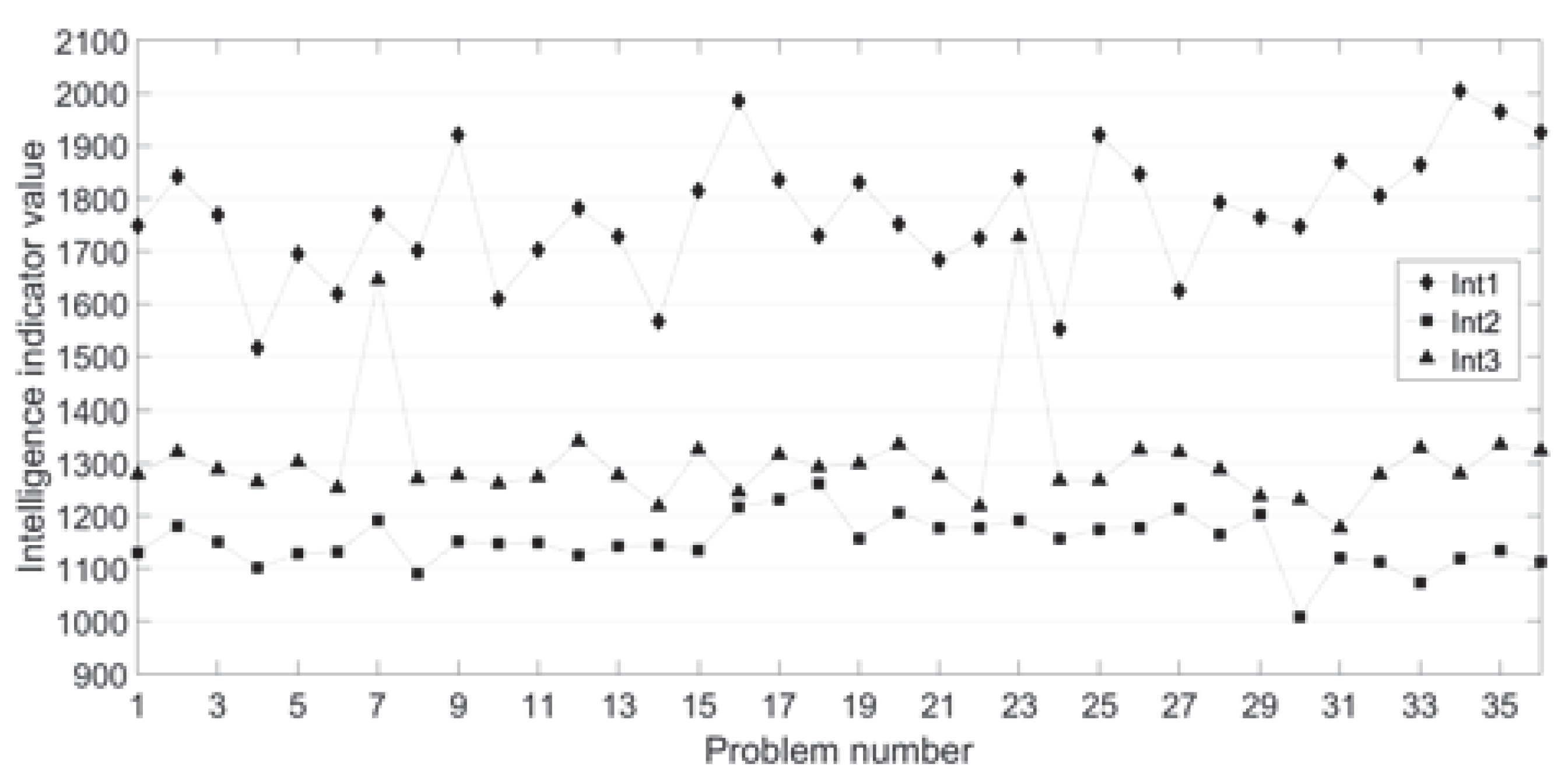
For intelligence measurement, a particular experimental setup was considered. Experiments were performed using a computing system with a Quad Core I7 2.6 GHz processor and 8 GB RAM. There were considered maps with nr = 100 randomly placed cities on the map. The most appropriate parameter values were considered based on some experimental evaluations. As parameters, for all the CMASs, the following settings were considered: number-of-steps = 1000; = 1 (power of the pheromone); = 1 (power of the distance/edge weight); = 0.1 (the evaporation factor). Table 3 presents a part of the obtained experimental intelligence evaluation results. Figure 2 provides a graphic representation of Int, Int, and Int. In the simulations, the obtained best-to-date travel value at the end of the problem-solving was considered as the intelligence indicator. A smaller value of the global-best has the significance of higher intelligence. Probl = {Prl, Prl, …, Prl} represents the set of problems used in the problem-solving intelligence evaluations.
Table 4 presents the results of the descriptive characterization of Int, Int, Int intelligence indicators samples, where mean denotes the sample mean; sample size represents the calculated sample size; LowerCI and UpperCI represent the lower and upper confidence interval of the sample mean; SD denotes the sample standard deviation; CV represents the coefficient of variation of the sample; variance represents the sample variance (calculated as ); min represents the smallest value from the sample; max represents the largest value of the sample; median represents the median of the sample.
Table 5 presents the results of the normality tests performed for Int, Int, Int. Table 6 presents the results of the descriptive characterization of Int, Int, Int intelligence indicators samples. Table 7 presents the results of the normality tests performed for Int, Int, Int. To check the normality of data, the KS, Lill, and SW tests were applied, all of them at the significance level αNorm = 0.05. Table 5 and Table 7 present, in the case of all the performed normality tests, the obtained test statistic and the p-value. For effective interpretation, only the p-value was used. The condition p-value > αNorm indicated the passing of the normality assumption at the considered significance level.
Table 4 and Table 5 present the results obtained by analyzing Int, Int, and Int data, where Table 4 presents a descriptive characterization, and Table 5 presents the results of normality testing. Not all the intelligence indicators’ data pass the normality assumption. Based on this fact, the Friedman test is applied with the chosen significance level αMore = 0.05. The obtained Friedman test p-value ≈ 0.0001 (Friedman Statistic Fr = 72 ), p-value <αMore, indicates that there is a statistically significant difference among the intelligence of Coop, Coop, and Coop. This means that all three CMASs cannot be included in the same class of intelligence. For further processing, the Dunn test with the significance level αPost = 0.05 (Table 8, the column labeled “Dunn test”) was used to compare all pairs of CMASs. For the interpretation of the results, the p-value of the Dunn test should be compared with the αPost significance level. p-value ≤Post indicates a significant statistical difference between a compared pair of CMASs. p-value ≤Post means that the two compared CMASs cannot be classified in the same class. The obtained results indicate that no couple of the studied CMASs can be included in the same class. Henceforth, there are three identified intelligence classes.
Applying the second approach of the MetrIntPairII algorithm, based on the fact that Int does not pass the normality assumption, extremes were identified using the Grubbs test on the Int intelligence indicator data. At the first application of the test, Int3 = 1727 corresponding to Pr was identified as an outlier. It was removed from Int,Int = Int−{Int3}, removing at the same time the corresponding values from Int(Int2 = 1192), Int = Int−{Int2} and Int(Int1 = 1839),Int = Int−{Int1}. The removal of Int2 and Int1 from Int and Int, respectively, was based on the pairing property (they were the intelligence indicators obtained as the Pr problem-solving intelligence evaluation by Coop and Coop). At the second application of the Grubbs test, Int3 = 1646 associated with Pr was identified as the second extreme. It was removed from Int,Int = Int−{Int3}, removing at the same time the corresponding values from Int (Int2 = 1191), Int = Int2−{Int2} and Int(Int1 = 1770),Int = Int−{Int1}. The removal of Int2 from Int and Int1 from Int was based on the pairing property.
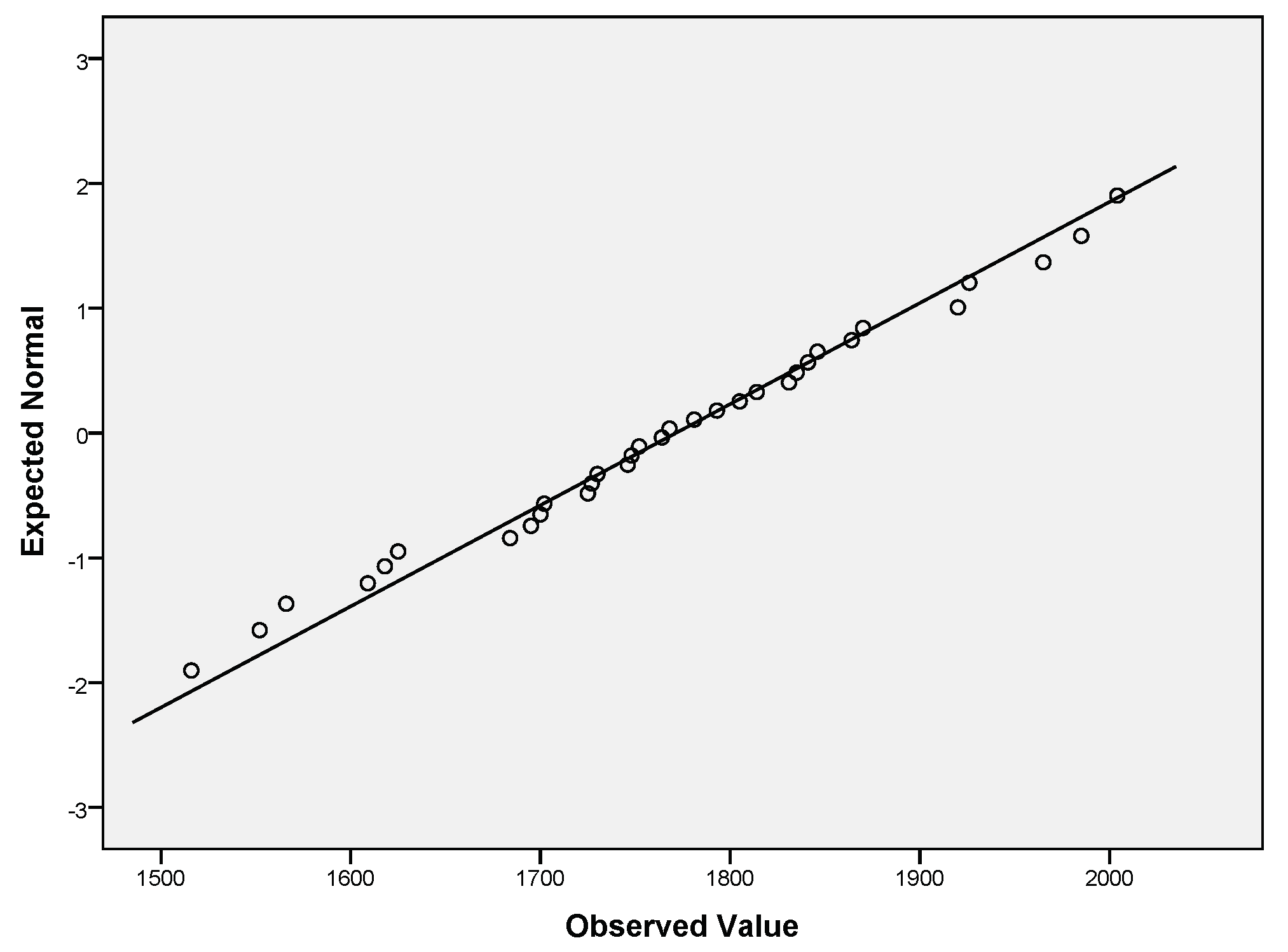
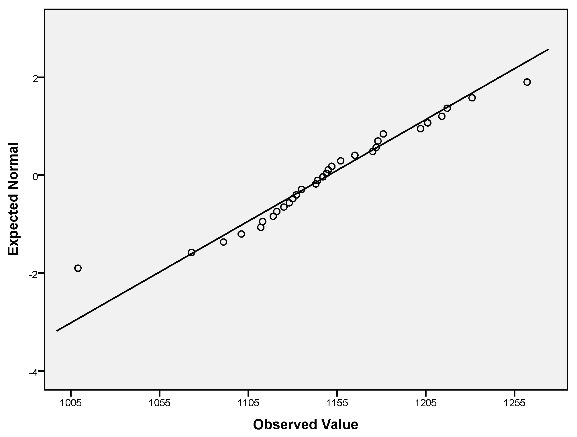
The obtained Int, Int, Int data passed the normality assumption (see Table 7 for the obtained normality test results and Table 6 for the performed descriptive characterization of intelligence indicators). QQ plots for Int (Figure 3), Int (Figure 4), Int (Figure 5) were constructed. The visual interpretation of Figure 3, Figure 4 and Figure 5 lead to the same conclusion that Int, Int, Int passed the normality assumption (the points fall approximately along this reference line).
Based on this fact, according to the MetrIntPairII algorithm, the application of the Repeated Measure Anovatest was considered with the significance level αMore = 0.05. The obtained p-value ≈ 0.0001 (p-value <αMore) indicated that the intelligence of the three studied CMASs present significant differences. Henceforth, Coop, Coop, and Coop cannot be included in the same class of intelligence. The fact that the p-value <αMore and all the intelligence indicators data Int, Int, Int passed the normality test justifies the application of Tukey–Kramer Multiple Comparisons testwith the significance level αPost = 0.05 for the comparison of all pairs of CMASs (Table 8, the column labeled “Tukey–Kramertest”). If p-value <αPost, then the two compared CMASs cannot be classified in the same class of intelligence. The final decision based on the obtained results presented in Table 8 indicates that all three studied CMASs should be assigned to different classes.
Table 8 indicates that the obtained results in both the parametric (applied Tukey–Kramer test) and the non-parametric (applied Dunn test) cases were the same. Based on the pairwise comparisons, it can be concluded that the difference in the intelligence of any two of the studied three CMASs is statistically significant. Henceforth, Coop, Coop, and Coop should be assigned to separate classes of intelligence. Coop belongs to the most intelligent class, denoted IntClass.Coop belongs to the second intelligence class, denoted IntClass. Coop belongs to the third intelligence class, denoted IntClass. The intelligence of CMASs that belong to IntClass is higher than the intelligence of the CMASs that belong to IntClass. The intelligence of CMASs that belong to IntClass is higher than the intelligence of the CMASs that belong to IntClass.
5. Discussion
Frequently, in CMASs, the intelligence can be considered at the system’s level. Although the intelligence of CMASs cannot be defined universally, it is useful to measure it. This is similar to the nature of human intelligence. Nobody deeply understands what human intelligence is, but even in this context, there are intelligence tests that can measure it. The outcome of human intelligence tests are useful for applicative purposes, such as the comparison of the effectiveness of two books used for learning by students taking the same exam. Each of the students uses one of the two books for learning. If the IQ of the students is taken into consideration in the comparison, more accurate results will be obtained, in the sense that a more intelligent student can learn easier even from a poorly written educational book.
There are few metrics presented in the scientific literature, where most of them is based on a specific ideology. The different ideology of the intelligence measuring does not allow a direct comparison of the metrics. In our study, intelligence measurement was considered based on the ability to solve difficult problems. The designed MetrIntPairII metric is appropriate for CMASs, where the intelligence indicator of the problem-solving ability of each CMAS can be expressed as a single value. If necessary (in the case of highly complex systems), this value can be computed as a weighted sum of other values that measure different aspects of the system’s intelligence. MetrIntPairII takes into consideration the variability in the intelligence of the compared CMASs. A CMAS may have a different value of intelligence in different situations. For a specific problem, the intelligence of a CMAS may be higher or lower. Extreme intelligence of CMASs was also considered with extreme high and low intelligence values. If such extreme intelligence indicator values are taken into consideration in case of a CMAS, they might strongly influence the value of its measured machine intelligence.
The MetrIntPairII algorithm, based on some mathematically grounded analysis, chooses the application of either the parametric Single-Factor ANOVA test with replications [60,61] or the nonparametric Friedmantest [62,63]. Based on this fact, the principal properties of the MetrIntPairII metric consist in accuracy and robustness in comparison and classification. In the case of our metric, if the intelligence indicator data pass the normality assumption, then the mean should be chosen as a representative statistical indicator of the central intelligence tendency. If the intelligence indicator data do not pass the normality assumption, then the median should be chosen as a representative statistical indicator of the central intelligence tendency based on the fact that is more robust than the mean. The robustness can be explained based on the fact that an extreme value (very high or very low) influences the median value in a lower degree than the value of the mean.
Another strength of the MetrIntPairII metric consists in the reduced sample size of necessary intelligence indicators, which is a result of using pairwise intelligence evaluations, such as the two sample paired and unpaired tests for the verification of the null hypothesis, which consists in the verification of equality of the means or medians of two samples. For example, an application can be considered in the following context: tails = 2 (in statistical analysis, the two-tailed test is almost always chosen instead the one-tailed test); = 0.05; = 0.2, Power = 1 − = 0.8; Effect size = 0.5. β is a type II error, the probability from failure to reject a false null hypothesis. Generally speaking, a type I error is the detection of an effect that is not present, while a type II error is failing to detect an effect that is present. An effect size is a quantitative measure of the strength of a phenomenon. The power represents the probability of detecting a true effect. Based on these data, using an a priori calculus (two samples) in a parametric case (normally distributed data), in the case of matched pairs, the sample size of each sample should be 34; in the case of non-matched pairs, the sample size of each sample should be 64.
A comparable metric called MetrIntPair was presented in [27]. MetrIntPair uses difficult-problem-solving intelligence measuring data. Based on that, it makes a mathematically grounded comparison of the intelligence of two CMASs at an application. Finally, it can classify the compared systems into intelligence classes. MetrIntPair is based on the same consideration for the pairwise measuring of difficult-problem-solving intelligence, similar to the MetrIntPairII metric introduced in this paper. MetrIntPairII conserves the properties of the MetrIntPair metric. The increased generality of the MetrIntPairII metric versus the MetrIntPair metric is the fact that MetrIntPairII is able to simultaneously compare and classify a large number of CMASs at an application. MetrIntPairII, at some point, uses the One-way Repeated Measure ANOVA test, a generalization of the Two-sample Paired T-test [60,61] (used by the MetrIntPairmetric). The Repeated Measure ANOVA test for two samples should yield results that are similar to the Two-sample Paired T-testfor two CMASs, considering that both tests are applied by taking into consideration all the requested assumptions. Based on this fact, the p-value of the One-way Repeated Measure ANOVA test is mathematically identical to the p-value of the Two-sample Paired T-test.
We applied the MetrIntPairII metric to the intelligence indicator data reported in [27]. The main purpose of the experimental comparison consisted in proving that the MetrIntPairII metric yields results that are similar to the MetrIntPair metric in the comparison of the intelligence of two CMASs. In [27], two CMASs specialized in solving a class of NP-hard problems were considered. One of them operated similarly to a Rank-Based Ant System(RB) [80,82], and the other operated as a Min-Max Ant System(MM) [79,80]. The experimentally compared two metrics led to the same decision regarding the intelligence of the studied CMASs.
The Family-wise error rate (FWER) is the probability of making one or more type I errors when performing multiple hypotheses tests [29]. If m-independent comparisons are performed, the FWER is calculated according to (13). Comp denotes the type I error of a single comparison. Ov denotes the overall type I error as a result of m comparisons.
MetrIntPair could be applied for the comparison of more than two CMASs, but this approach would not be appropriate. The probability of making a type I error increases as the number of tests increase. If the significance level is set at , the probability of a type I error can be obtained, regardless of the number of groups being compared. For instance, if the probability of a type I error for the analysis is set at = 0.05 and four two sample tests (T-test for example) are performed, the overall probability of a type I error for the set of tests Ov = 1 − 0.95≈ 0.186 (0.185494) substantially increases. In the case of MetrIntPairII for the same four intelligence samples, the type I error does not change. Its value remains at 0.05. In the case of MetrIntPairII,the probability of making a type I error does not increase as the number of compared systems increases.
The extension of the MetrIntPairII metric versus the MetrIntPair consists in using a statistical non-parametric test for intelligence indicator data that do not pass the normality assumption. In this case, it uses the Friedman test, which is known as a robust nonparametric test [62,63]. MetrIntPairII based on the obtained intelligence indicators makes a mathematically grounded analysis and applies the most appropriate statistical tests.
6. Conclusions
In this paper, a novel intelligence metric called MetrIntPairII was proposed. MetrIntPairII is able to make an effective measuring and comparison of the intelligence of several CMASs. Based on their difficult-problem-solving intelligence, the studied CMASs are classified into intelligence classes. MetrIntPairII is accurate and robust based on the fact that it takes into account the variability in the intelligence of the compared CMAS and the occurrence of extreme (low and high) intelligence measurement results. MetrIntPairII is a generalization and extension of the metric called MetrIntPair, presented in the scientific literature.
For validation purposes, we performed experimental difficult-problem-solving intelligence evaluations for a set of CMASs. Each CMAS was composed of simple computing agents specialized in solving an NP-hard problem, in that, at the systems’ level, increased intelligence emerged.
The most important property of the proposed metric that suggests its applicability is its universality. MetrIntPairII was presented as being applied for CMASs. This decision was based on the fact that measuring the intelligence of a CMASs is usually more difficult than measuring the intelligence of a system that operates individually. MetrIntPairII can be applied to intelligent agent-based systems generally, even to systems that operate in isolation without cooperating with other systems during problem-solving. Prospective applications could include the intelligence measuring of robotics swarms. It can provide a reliable comparison, for instance, of the intelligence of a set of agents with different architectures that solve problems in isolation with the intelligence of a cooperative coalition of agents in solving the same type of problem. Based on a comprehensive scientific literature review performed in this study, the metric proposed in this paper is original, and we estimate that it will represent the foundation for the intelligence measuring of IABSs in many future studies.
Funding
This research received no external funding.
Institutional Review Board Statement
Not applicable.
Informed Consent Statement
Not applicable.
Data Availability Statement
Not applicable.
Acknowledgments
This work was developed in the framework of the CHIST-ERA programme supported by the Future and Emerging Technologies (FET) programme of the European Union through the ERA-NET Cofund funding scheme under the grant agreements, title: Social Network of Machines (SOON). This research was supported by a grant of the Romanian National Authority for Scientific Research and Innovation, CCCDI-UEFISCDI, project number 101/2019, COFUND-CHIST-ERA-SOON, within PNCDI III.
Conflicts of Interest
The author declares no conflict of interest.
References
- Yang, K.; Galis, A.; Guo, X.; Liu, D. Rule-driven mobile intelligent agents for real-time configuration of IP networks. In Knowledge-Based Intelligent Information and Engineering Systems; Palade, V., Howlett, R.J., Jain, L., Eds.; Springer: Berlin/Heidelberg, Germany, 2003; Volume 2773, pp. 921–928. [Google Scholar]
- Iantovics, L.B.; Zamfirescu, C.B. ERMS: An Evolutionary Reorganizing Multiagent System. Int. J. Innov. Comput. 2013, 9, 1171–1188. [Google Scholar]
- Graziano, M.G. Fuzzy cooperative behavior in response to market imperfections. Int. J. Intell. Syst. 2012, 27, 108–131. [Google Scholar] [CrossRef]
- Jumadinova, J.; Dasgupta, P. A multi-agent system for analyzing the effect of information on prediction markets. Int. J. Intell. Syst. 2011, 26, 383–409. [Google Scholar] [CrossRef]
- Huang, Z.; Kim, J.; Sadri, A.; Dowey, S.; Dargusch, M.S. Industry 4.0: Development of a multi-agent system for dynamic value stream mapping in SMEs. J. Manuf. Syst. 2019, 52, 1–12. [Google Scholar] [CrossRef]
- Grachev, S.; Skobelev, P.; Mayorov, I.; Simonova, E. Adaptive Clustering through Multi-Agent Technology: Development and Perspectives. Mathematics 2020, 8, 1664. [Google Scholar] [CrossRef]
- Lanza, G.; Patti, D.M.A.; Navarra, P. Can Citizens Affect the Performance of Their Elected Representatives? A Principal-Agent Model of Strategic Interaction in Democratic Systems. Mathematics 2020, 8, 1194. [Google Scholar] [CrossRef]
- Chen, Y.T.; Cao, Z.C. An Investigation on a Closed-Loop Supply Chain of Product Recycling Using a Multi-Agent and Priority Based Genetic Algorithm Approach. Mathematics 2020, 8, 888. [Google Scholar] [CrossRef]
- Tran, M.T.; Duong, D.; Pham-Hi, D.; Bui, M. Detecting the Proportion of Traders in the Stock Market: An Agent-Based Approach. Mathematics 2020, 8, 198. [Google Scholar] [CrossRef] [Green Version]
- Lin, Z. Control design in the presence of actuator saturation: From individual systems to multi-agent systems. Sci. China Inf. Sci. 2019, 62, 26201. [Google Scholar] [CrossRef] [Green Version]
- Coelho, C.G.C.; Abreu, C.G.; Ramos, R.M.; Mendes, A.H.D.; Teodoro, G.; Ralha, C.G. MASE-BDI: Agent-based simulator for environmental land change with efficient and parallel auto-tuning. Appl. Intell. 2016, 45, 904–922. [Google Scholar] [CrossRef]
- Wang, Y.; Tao, R.; Zhang, H. Research on distributed intrusion detection system based on multi-living agent. Sci. China Inf. Sci. 2010, 53, 1067–1077. [Google Scholar] [CrossRef]
- Wang, Y.; Tao, R.; Li, B. Using the multi-living agent concept to investigate complex information systems. Sci. China Ser. F Inf. Sci. 2009, 52, 1–17. [Google Scholar] [CrossRef]
- Celik, D.; Elci, A. A broker-based semantic agent for discovering Semantic Web services through process similarity matching and equivalence considering quality of service. Sci. China Inf. Sci. 2013, 56, 1–24. [Google Scholar] [CrossRef] [Green Version]
- Manickam, A.; Kamalasadan, S.; Edwards, D.; Simmons, S. A Novel Self-Evolving Intelligent Multiagent Framework for Power System Control and Protection. IEEE Syst. J. 2014, 8, 1086–1095. [Google Scholar] [CrossRef]
- Harati, A.; Ahmadabadi, M.N.; Araabi, B.N. Knowledge-Based Multiagent Credit Assignment: A Study on Task Type and Critic Information. IEEE Syst. J. 2007, 1, 55–67. [Google Scholar] [CrossRef]
- Chouhan, S.S.; Niyogi, R. MAPJA: Multi-agent planning with joint actions. Appl. Intell. 2017, 47, 1044–1058. [Google Scholar] [CrossRef]
- Hsieh, F.S. A hybrid and scalable multi-agent approach for patient scheduling based on Petri net models. Appl. Intell. 2017, 7, 1068–1086. [Google Scholar] [CrossRef]
- Sharpanskykh, A.; Haest, R. An agent-based model to study compliance with safety regulations at an airline ground service organization. Appl. Intell. 2016, 45, 881–903. [Google Scholar] [CrossRef] [Green Version]
- Li, X.; Zhang, H. A multi-agent complex network algorithm for multi-objective optimization. Appl. Intell. 2020, 50, 2690–2717. [Google Scholar] [CrossRef]
- Labati, R.D.; Genovese, A.; Muñoz, E.; Piuri, V.; Scotti, F.; Sforza, G. Computational intelligence for industrial and environmental applications. In Proceedings of the IEEE 8th International Conference on Intelligent Systems (IS), Sofia, Bulgaria, 4–6 September 2016; pp. 8–14. [Google Scholar]
- Scotti, F.; Piuri, V. Adaptive Reflection Detection and Location in Iris Biometric Images by Using Computational Intelligence Techniques. IEEE Trans. Instrum. Meas. 2010, 59, 1825–1833. [Google Scholar] [CrossRef]
- Piuri, V.; Sami, M.; Stefanelli, R. Arithmetic codes for concurrent error detection in artificial neural networks: The case of AN+B codes. In Proceedings of the IEEE International Workshop on Defect and Fault Tolerance in VLSI Systems, Dallas, TX, USA, 4–6 November 1992; pp. 127–136. [Google Scholar]
- Iakovidis, D.K.; Papageorgiou, E. Intuitionistic fuzzy cognitive maps for medical decision making. IEEE Trans. Inf. Technol. Biomed. 2011, 15, 100–107. [Google Scholar] [CrossRef]
- Papageorgiou, E.I.; Iakovidis, D.K. Intuitionistic fuzzy cognitive maps. IEEE Trans. Fuzzy Syst. 2013, 21, 342–354. [Google Scholar] [CrossRef]
- Meystel, A.M.; Messina, E.R. Measuring the Performance and Intelligence of Systems. In Proceedings of the 2000 PerMIS Workshop, Gaithersburg, MD, USA, 14–16 August 2000; National Institute of Standards and Technology, Special Publication 970. U.S. Government Printing Office: Washington, DC, USA, 2001. [Google Scholar]
- Iantovics, L.B.; Rotar, C.; Niazi, M.A. MetrIntPair—A novel accurate metric for the comparison of two cooperative multiagent systems intelligence based on paired intelligence measurements. Int. J. Intell. Syst. 2018, 33, 463–486. [Google Scholar] [CrossRef]
- Iantovics, L.B.; Rotar, C.; Nechita, E. A novel robust metric for comparing the intelligence of two cooperative multiagent systems. Procedia Comput. Sci. 2016, 96, 637–644. [Google Scholar] [CrossRef] [Green Version]
- Bartroff, J.; Song, J. Sequential Tests of Multiple Hypotheses Controlling Type I and II Familywise Error Rates. J. Stat. Plan. Inference 2014, 153, 100–114. [Google Scholar] [CrossRef] [PubMed] [Green Version]
- Turing, A.M. Computing machinery and intelligence. Mind 1950, 59, 433–460. [Google Scholar] [CrossRef]
- Sabzi, H.Z.; King, J.P.; Abudu, S. Developing an intelligent expert system for streamflow prediction, integrated in a dynamic decision support system for managing multiple reservoirs: A case study. Expert Syst. Appl. 2017, 83, 145–163. [Google Scholar] [CrossRef]
- Sterret, S.G. Turing on the Integration of Human and Machine Intelligence. In Philosophical Explorations of the Legacy of Alan Turing; Floyd, J., Bokulich, A., Eds.; Boston Studies in the Philosophy and History of Science; Springer: Cham, Switzerland, 2017; Volume 324, pp. 323–338. [Google Scholar]
- Newborn, M. Kasparov Vs. Deep Blue: Computer Chess Comes of Age; Springer: New York, NY, USA, 1997. [Google Scholar]
- Besold, T.; Hernandez-Orallo, J.; Schmid, U. Can Machine Intelligence be Measured in the Same Way as Human intelligence? Künstliche Intell. 2015, 29, 291–297. [Google Scholar] [CrossRef] [Green Version]
- Detterman, D.K. A challenge to Watson. Intelligence 2011, 39, 77–78. [Google Scholar] [CrossRef]
- Sanghi, P.; Dowe, D.L. A computer program capable of passing I.Q. tests. In Proceedings of the Joint International Conference on Cognitive Science, 4th ICCS International Conference on Cognitive Science and 7th ASCS Australasian Society for Cognitive Science, Sydney, Australia, 13–17 July 2003; pp. 570–575. [Google Scholar]
- Iantovics, L.B.; Dehmer, M.; Emmert-Streib, F. MetrIntSimil—An Accurate and Robust Metric for Comparison of Similarity in Intelligence of Any Number of Cooperative Multiagent Systems. Symmetry 2018, 10, 48. [Google Scholar] [CrossRef] [Green Version]
- Schreiner, K. Measuring IS: Toward a US standard. IEEE Intell. Syst. Their Appl. 2000, 15, 19–21. [Google Scholar] [CrossRef]
- Park, H.J.; Kim, B.K.; Lim, K.Y. Measuring the machine intelligence quotient (MIQ) of human-machine cooperative systems. IEEE Trans. Syst. Man Cybern. Part A Syst. Hum. 2001, 31, 89–96. [Google Scholar] [CrossRef]
- Anthon, A.; Jannett, T.C. Measuring machine intelligence of an agent-based distributed sensor network system. In Advances and Innovations in Systems, Computing Sciences and Software Engineering; Elleithy, K., Ed.; Springer: Dordrecht, The Netherlands, 2007; pp. 531–535. [Google Scholar]
- Hernández-Orallo, J.; Dowe, D.L. Measuring universal intelligence: Towards an anytime intelligence test. Artif. Intell. 2010, 174, 1508–1539. [Google Scholar] [CrossRef] [Green Version]
- Iantovics, L.B.; Kountchev, R.; Crisan, G.C. ExtrIntDetect—A New Universal Method for the Identification of Intelligent Cooperative Multiagent Systems with Extreme Intelligence. Symmetry 2019, 11, 1123. [Google Scholar] [CrossRef] [Green Version]
- Legg, S.; Hutter, M. A formal measure of machine intelligence. In Proceedings of the 15th Annual Machine Learning Conference of Belgium and The Netherlands, Ghent, Belgium, 11–12 May 2006; pp. 73–80. [Google Scholar]
- Hibbard, B. Measuring agent intelligence via hierarchies of environments. In Artificial General Intelligence; Schmidhuber, J., Thórisson, K.R., Looks, M., Eds.; Springer: Berlin/Heidelberg, Germany, 2011; pp. 303–308. [Google Scholar]
- Liu, F.; Shi, Y.; Liu, Y. Intelligence quotient and intelligence grade of artificial intelligence. Ann. Data Sci. 2017, 4, 179–191. [Google Scholar] [CrossRef] [Green Version]
- Iantovics, L.B.; Emmert-Streib, F.; Arik, S. MetrIntMeas a novel metric for measuring the intelligence of a swarm of cooperating agents. Cogn. Syst. Res. 2017, 45, 17–29. [Google Scholar] [CrossRef]
- Iantovics, L.B.; Kovács, L.; Rotar, C. MeasApplInt—A novel intelligence metric for choosing the computing systems able to solve real-life problems with a high intelligence. Appl. Intell. 2019, 49, 3491–3511. [Google Scholar] [CrossRef]
- Razali, N.; Wah, Y.B. Power comparisons of Shapiro-Wilk, Kolmogorov-Smirnov, Lilliefors and Anderson-Darling tests. J. Stat. Model. Anal. 2011, 2, 21–33. [Google Scholar]
- Stephens, M.A. EDF statistics for goodness of fit and some comparisons. J. Am. Stat. Assoc. 1974, 69, 730–737. [Google Scholar] [CrossRef]
- Chakravarti, I.M.; Laha, R.G.; Roy, J. Handbook of Methods of Applied Statistics; Wiley: New York, NY, USA, 1967; Volume I, pp. 392–394. [Google Scholar]
- Lilliefors, H. On the Kolmogorov-Smirnov test for normality with mean and variance unknown. J. Am. Stat. Assoc. 1967, 62, 399–402. [Google Scholar] [CrossRef]
- Lilliefors, H. On the Kolmogorov-Smirnov test for the exponential distribution with mean unknown. J. Am. Stat. Assoc. 1969, 64, 387–389. [Google Scholar] [CrossRef]
- Dallal, G.E.; Wilkinson, L. An analytic approximation to the distribution of Lilliefors’s test statistic for normality. Am. Stat. 1986, 40, 294–296. [Google Scholar]
- Shapiro, S.S.; Wilk, M.B. An analysis of variance test for normality (complete samples). Biometrika 1965, 52, 591–611. [Google Scholar] [CrossRef]
- Barnett, V.; Lewis, T. Outliers in Statistical Data, 3rd ed.; Wiley: New York, NY, USA, 1994. [Google Scholar]
- Stefansky, W. Rejecting outliers in factorial designs. Technometrics 1972, 14, 469–479. [Google Scholar] [CrossRef]
- Grubbs, F.E. Sample criteria for testing outlying observations. Ann. Math. Stat. 1950, 21, 27–58. [Google Scholar] [CrossRef]
- Grubbs, F.E. Procedures for Detecting Outlying Observations in Samples. Technometrics 1969, 11, 1–21. [Google Scholar] [CrossRef]
- Motulsky, H. GraphPad InStat Version 3. In The Instat Guide to Choosing and Interpreting Statistical Tests; GraphPad Software, Inc.: San Diego, CA, USA, 2003. [Google Scholar]
- Muller, B. Approximate power for repeated-measures ANOVA lacking sphericity. J. Am. Stat. Assoc. 1989, 84, 549–555. [Google Scholar] [CrossRef]
- Gueorguieva, R.; Krystal, J.H. Move over ANOVA: Progress in analyzing repeated-measures data and its reflection in papers published in the Archives of General Psychiatry. Arch. Gen. Psychiatry 2004, 61, 310–317. [Google Scholar] [CrossRef]
- Friedman, M. The use of ranks to avoid the assumption of normality implicit in the analysis of variance. J. Am. Stat. Assoc. 1937, 32, 675–701, Correction in 1939, 34, 109. [Google Scholar] [CrossRef]
- Friedman, M. A comparison of alternative tests of significance for the problem of m rankings. Ann. Math. Stat. 1940, 11, 86–92. [Google Scholar] [CrossRef]
- Morrison, S.; Sosnoff, J.J.; Heffernan, K.S.; Jae, S.Y.; Fernhall, B. Aging, hypertension and physiological tremor: The contribution of the cardioballistic impulse to tremorgenesis in older adults. J. Neurol. Sci. 2013, 326, 68–74. [Google Scholar] [CrossRef] [PubMed]
- Tukey, J. Comparing individual means in the analysis of variance. Biometrics 1949, 5, 99–114. [Google Scholar] [CrossRef] [PubMed]
- Siegel, S.; Castellan, N.J. Nonparametric Statistics for the Behavioral Sciences; McGraw-Hill: New York, NY, USA, 1988. [Google Scholar]
- Dunn, O.J. Multiple Comparisons Using Rank Sums. Technometrics 1964, 6, 241–252. [Google Scholar] [CrossRef]
- Dorigo, M.; Maniezzo, V.; Colorni, A. Positive Feedback As a Search Strategy; Technical Report 91-016; Dipartimento di Elettronica, Politecnico di Milano: Milan, Italy, 1991. [Google Scholar]
- Colorni, A.; Dorigo, M.; Maniezzo, V. Distributed optimization by ant colonies. In European Conference on Artificial Life; Varela, F., Bourgine, P., Eds.; Elsevier: Paris, France, 1991; pp. 134–142. [Google Scholar]
- Dorigo, M. Optimization, Learning and Natural Algorithms. Ph.D. Thesis, Dipartimento di Elettronica, Politecnico di Milano, Milan, Italy, 1992. (In Italian). [Google Scholar]
- Dorigo, M.; Maniezzo, V.; Colorni, A. Ant System: Optimization by a colony of cooperating agents. IEEE Trans. Syst. Man Cybern. Part B 1996, 26, 29–41. [Google Scholar] [CrossRef] [Green Version]
- Beni, G.; Wang, J. Swarm Intelligence in Cellular Robotic Systems, Proceed. In Proceedings of the NATO Advanced Workshop on Robots and Biological Systems, Tuscany, Italy, 26–30 June 1993. [Google Scholar]
- Wilson, S.; Pavlic, T.P.; Kumar, G.P.; Buffin, A.; Pratt, S.C.; Berman, S. Design of ant-inspired stochastic control policies for collective transport by robotic swarms. Swarm Intell. 2014, 8, 303–327. [Google Scholar] [CrossRef] [Green Version]
- Berman, S.; Halasz, A.; Kumar, V.; Pratt, S. Algorithms for the Analysis and Synthesis of a Bio-inspired Swarm Robotic System. In Swarm Robotics. SR 2006. Lecture Notes in Computer Science; Sahin, E., Spears, W.M., Winfield, A.F.T., Eds.; Springer: Berlin/Heidelberg, Germany, 2007; Volume 4433, pp. 56–70. [Google Scholar]
- Ducatelle, F.; Di Caro, G.A.; Pinciroli, C.; Gambardella, L.M. Self-organized cooperation between robotic swarms. Swarm Intell. 2011, 5, 73. [Google Scholar] [CrossRef]
- Cordon, O.; Herrera, F.; de Viana, I.F.; Moreno, L. A New ACO Model Integrating Evolutionary Computation Concepts: The Best-Worst Ant System. In Proceedings of the ANTS’2000. From Ant Colonies to Artificial Ants: Second International Workshop on Ant Algorithms, Brussels, Belgium, 7–9 September 2000; pp. 22–29. [Google Scholar]
- Cordon, O.; de Viana, I.F.; Herrera, F. Analysis of the Best-Worst Ant System and Its Variants on the QAP. In Ant Algorithms; Dorigo, M., Di Caro, G., Sampels, M., Eds.; Springer: Berlin/Heidelberg, Germany, 2002; Volume 2463, pp. 228–234. [Google Scholar]
- Zhang, Y.; Wang, H.; Zhang, Y.; Chen, Y. Best-worst ant system. In Proceedings of the 3rd International Conference on Advanced Computer Control (ICACC), Harbin, China, 18–20 January 2011; pp. 392–395. [Google Scholar]
- Stützle, T.; Hoos, H.H. Max-min ant system. Future Gener. Comput. Syst. 2000, 16, 889–914. [Google Scholar] [CrossRef]
- Prakasam, A.; Savarimuthu, N. Metaheuristic algorithms and probabilistic behaviour: A comprehensive analysis of Ant Colony Optimization and its variants. Artif. Intell. Rev. 2016, 45, 97–130. [Google Scholar] [CrossRef]
- Dorigo, M.; Gambardella, L.M. Ant Colony System: A cooperative learning approach to the traveling salesman problem. IEEE Trans. Evol. Comput. 1997, 1, 53–66. [Google Scholar] [CrossRef] [Green Version]
- Bullnheimer, B.; Hartl, R.F.; Strauss, C. A new rank based version of the Ant System. A computational study. Cent. Eur. J. Oper. Res. 1999, 7, 25–38. [Google Scholar]
Figure 1.
Main processing performed by the Algorithm 1.

Figure 2.
Graphical representation of Int, Int and Int.

Figure 3.
QQ plot of Int.

Figure 4.
QQ plot of Int.

Figure 5.
QQ plot of Int.


Table 1.
Results of the problem-solving intelligence evaluation.
| Probl | Int | Int | .. | Int | Formed Pairs |
|---|---|---|---|---|---|
| Prl | In1 | In2 | Inm | In1-In2-…- Inm | |
| Prl | In1 | In2 | Inm | In1-In2-…- Inm | |
| …… | …… | …… | |||
| Prl | In1 | In2 | Inm | In1-In2-…- Inm | |
| MIQ | MIQ | MIQ |
Table 2.
Transformation to obtain normally distributed data.
| IN Type - Distribution | Normalizing Transformation |
|---|---|
| Poisson distribution | SquareRoot(IN) |
| Time or Duration | 1/IN |
| Lognormal distribution | Log(IN) |
| Binomial distribution | Arcsine(SquareRoot(IN)) |
Table 3.
Intelligence indicators for Coop/Int, Coop/Int, and Coop/Int.
| Int | Int | Int |
|---|---|---|
| In1(1748); In1(1841);… | In2(1130);In2(1181);… | In3(1278);In3(1322);… |
| In1(1770); In1(1700);In1(1920); | In2(1191);In2(1091); | In3(1646);In3(1271); |
| In1(1609); …In1(1839); | In2(1152);In2(1147);… | In3(1277); In3(1262);… |
| … | In2(1192); … | In3(1727);… |
Table 4.
Results of the Int, Int, Int analysis.
| Int | Int | Int | |
|---|---|---|---|
| mean/ sample size | 1773.22/36 | 1152.56/36 | 1304.89/36 |
| LowerCI/ UpperCI | 1732.5/1814 | 1136.4/1168.7 | 1270.5/1339.3 |
| SD/ CV | 120.39/6.79 | 47.7/4.14 | 101.61/7.79 |
| variance | 14,493.95 | 2275.28 | 10,324.56 |
| min/ max | 1616/2004 | 1009/1262 | 1177/1727 |
| median | 1769 | 1149.5 | 1279 |
Table 5.
Results of normality testing for Int, Int, Int.
| Int | Int | Int | |
|---|---|---|---|
| KS Stat/p-value | 0.067/ ≈ 0.1 | 0.087/ ≈ 0.1 | 0.30/0.001 |
| Lill Stat/p-value | 0.67/ ≈ 0.2 | 0.86/ ≈ 0.2 | 0.302/0 |
| SW Stat/p-value | 0.93/ ≈ 0.851 | 0.976/ ≈ 0.67 | 0.612/0 |
| Normality passed | Yes | Yes | No |
Table 6.
Results of the Int, Int, Int analysis.
| Int | Int | Int | |
|---|---|---|---|
| mean/ sample size | 1771.38/34 | 1150.26/34 | 1282.44/34 |
| LowerCI/ UpperCI | 1728.3/1814.5 | 1133.5/1167.1 | 1268.9/1296 |
| SD/ CV | 123.44/6.97 | 48.12/4.18 | 38.81/3.03 |
| variance | 15237.46 | 2315.84 | 1505.83 |
| min/ max | 1516/2004 | 1009/1262 | 1177/1278 |
| median | 1766 | 1148 | 1342 |
Table 7.
Results of the normality testing Int, Int, Int.
| Int | Int | Int | |
|---|---|---|---|
| KS Stat/p-value | 0.063/ ≈ 0.1 | 0.096/ ≈ 0.1 | 0.1/ ≈ 0.1 |
| Lill Stat/p-value | 0.63/ ≈ 0.2 | 0.968/ ≈ 0.2 | 0.1/ ≈ 0.2 |
| SW Stat/p-value | 0.983/0.873 /see Figure 3 | 0.972/≈0.505/see Figure 4 | 0.954/0.166/see Figure 5 |
| Normality passed | Yes | Yes | Yes |
Table 8.
Results of the Dunn and Tukey–Kramer post-hoc tests, post = 0.05.
| Dunn Test | Tukey–Kramer Test | ||||
|---|---|---|---|---|---|
| Rank Sum Difference | p-Value | Mean Difference | Q | p-Value | |
| Intvs. Int | 72 | <0.001 | 621.12 | 47.508 | <0.001 |
| Intvs. Int | 36 | <0.001 | 488.94 | 37.398 | <0.001 |
| Intvs. Int | −36 | <0.001 | −132.18 | 10.110 | <0.001 |
Publisher’s Note: MDPI stays neutral with regard to jurisdictional claims in published maps and institutional affiliations. |
© 2021 by the author. Licensee MDPI, Basel, Switzerland. This article is an open access article distributed under the terms and conditions of the Creative Commons Attribution (CC BY) license (http://creativecommons.org/licenses/by/4.0/).
Share and Cite
MDPI and ACS Style
Iantovics, L.B. Black-Box-Based Mathematical Modelling of Machine Intelligence Measuring. Mathematics 2021, 9, 681. https://doi.org/10.3390/math9060681
AMA Style
Iantovics LB. Black-Box-Based Mathematical Modelling of Machine Intelligence Measuring. Mathematics. 2021; 9(6):681. https://doi.org/10.3390/math9060681
Chicago/Turabian StyleIantovics, László Barna. 2021. "Black-Box-Based Mathematical Modelling of Machine Intelligence Measuring" Mathematics 9, no. 6: 681. https://doi.org/10.3390/math9060681
Note that from the first issue of 2016, this journal uses article numbers instead of page numbers. See further details here.