Article

Personalized Cotesting Policies for Cervical Cancer Screening: A POMDP Approach

by
Malek Ebadi
1,† and
Raha Akhavan-Tabatabaei
2,*,†
1
Faculty of Engineering and Natural Sciences, Sabanci University, Orta Mahalle, Tuzla 34956, Turkey
2
Sabanci Business School, Sabanci University, Orta Mahalle, Tuzla 34956, Turkey
*
Author to whom correspondence should be addressed.
These authors contributed equally to this work.
Mathematics 2021, 9(6), 679; https://doi.org/10.3390/math9060679
Submission received: 4 February 2021 / Revised: 15 March 2021 / Accepted: 16 March 2021 / Published: 22 March 2021
(This article belongs to the Special Issue Markov-Chain Modelling and Applications)

Abstract

:
Screening for cervical cancer is a critical policy that requires clinical and managerial vigilance because of its serious health consequences. Recently the practice of conducting simultaneous tests of cytology and Human Papillomavirus (HPV)-DNA testing (known as cotesting) has been included in the public health policies and guidelines with a fixed frequency. On the other hand, personalizing medical interventions by incorporating patient characteristics into the decision making process has gained considerable attention in recent years. We develop a personalized partially observable Markov decision process (POMDP) model for cervical cancer screening decisions by cotesting. In addition to the merits offered by the guidelines, by availing the possibility of including patient-specific risks and other attributes, our POMDP model provides a patient-tailored screening plan. Our results show that the policy generated by the POMDP model outperforms the static guidelines in terms of quality-adjusted life years (QALY) gain, while performing comparatively equal in lifetime risk reduction.

1. Introduction

Cervical cancer is the fourth most common cancer type among women worldwide [1]. Every year, more than half a million women are diagnosed with cervical cancer and over 300,000 cases result in death worldwide [2]. In nearly all of the cervical cancer cases an infection by Human Papillomavirus (HPV) is identified [3,4]. HPV is a sexually transmitted virus and spans a wide range of strains [5]. Two specific strains of HPV namely 16 and 18 are persistent in the body while the majority of the other strains are acute (non-persistent), harmless and cleaned from the body without medical interventions [6]. In this regard, spontaneous regression is a unique characteristic of the disease distinguishing it from most of the other cancer types.
The preclinical phase of cervical cancer is long; the virus remains silent for a long time and an infected woman may remain asymptomatic for several years before developing cancer [7]. Hence, the extended period from infection until the infected cells become cancerous creates a relatively high opportunity for detection and treatment of the cancer [8]. During the long asymptomatic period of the disease, it is critical to detect the infection and precancerous symptoms early enough in order to reduce the disease burden. Accomplishing this goal is possible either by preventive methods such as vaccination or by organized screening programs [9]. From the medical point of view, the uptake of HPV vaccine provides partial immunity against certain high risk strains and does not obviate the need for routine screening programs [10,11,12]. Hence, screening with one of the common tests namely cytology, HPV-DNA testing, and the practice of conducting both tests simultaneously (known as cotesting) should still remain in practice to prevent the disease.
Cytology-based screening (including conventional Pap smear and recent liquid based cytology) makes use of cytology to identify women at increased risk of cervical pathology by taking samples from the cervix and checking for precancerous abnormalities [13]. HPV-DNA testing on the other hand, refers to a broad class of testing methods, which rely on identification of HPV viral DNA. Specifically, qualitative methods detect only the presence or absence of HPV DNA; quantitative methods estimate the viral load as the quantity of virus in a given volume and some methods detect the degree of integration of HPV into the host genome [14].
Selection of the appropriate screening method depends on multiple attributes including age, prior screening records, availability of resources and test characteristics defined by its sensitivity and specificity [15]. Sensitivity of a test represents the fraction of patients with cancer having a positive test result and specificity of a test represents the fraction of healthy patients having a negative test result. A cytology test has a higher specificity but lower sensitivity compared to the HPV-DNA testing [16]. Low sensitivity results in a higher number of false negatives; hence, missing many precancerous lesions. To compensate this shortcoming of cytology, more frequent screenings at shorter intervals must be exercised, which could be infeasible in many countries and settings [17]. Conversely, HPV-DNA testing is more sensitive and hence, more suitable to detect the precancerous lesions that may be missed by cytology screening. HPV-DNA testing allows extending the screening intervals longer than those by cytology screening [18,19]. However, the lower specificity of HPV-DNA testing results in an increase in the number of false positive cases, which subsequently increases the costs by too many unnecessary follow-up tests [20,21]. Achieving a reasonable trade-off becomes even more challenging, knowing that in many cases, the precancerous lesions that are missed by cytology and found by HPV-DNA testing are clinically important [10]. Therefore, in many countries, the recommended screening modality is cotesting, which helps to maintain high sensitivity at longer intervals.
Since the disease evolves through time, women need to undergo screening regularly. There is now substantial and consistent evidence that the incidence of the disease has decreased sharply in the countries where regular population-based screening programs are implemented [22]. Such countries provide guidelines to inform the population about the frequency and timings of the screening rounds. In the US, the current guidelines of the American Cancer Society (ACS), the American Society for Colposcopy and Cervical Pathology (ASCCP), the American Society for Clinical Pathology (ASCP), and US Preventive Services Task Force (USPSTF) agree that regardless of the vaccination status, screening should start at the age of 21, and until 29 cytology to be conducted every three years. From age 30 until 65 cotesting every 5 years is preferred [23,24].
There are several advantages to following such static guidelines, including simplicity of implementation and effectiveness in reducing mortality. While guidelines create a distinct advantage by reducing the disease burden in many countries, they also suffer from several drawbacks. First, it is widely acknowledged that screening the whole population with the same intensive frequency is costly to the healthcare system and requires considerable availability of diverse resources and infrastructure [25]. Second, it must be recognized that the clinical understanding of cervical cancer is not static, rather it is exposed to fast-paced changes with the new emerging technologies [23]. Consequently, the population based guidelines very often evolve with the emergence of new data and evidence regarding the natural history of the disease and the optimal screening strategies [15]. In the United States, since the introduction of the first guideline, the guidelines have gone through several revisions [26]. This creates complexity and challenges to implement such guidelines in a context where a long chain of patients, healthcare providers, clinicians, gynecologists as well as healthcare payers have to continuously adapt to the frequent updates of the recommendations from the multiple guidelines [27].
As an alternative to the guidelines, personalized screening programs provide many advantages including the identification of the optimal intervention choice for distinct patient profiles, preventing adverse effects and reducing the overall healthcare costs [28]. Given that the current cervical screening guidelines are inflexible to differentiate between patient groups with distinct risk factors, we aim to develop a personalized model that can incorporate the cancer risk as well as test characteristics to create a patient-tailored screening program. Since a number of studies address the positive effect of applying cotesting as the primary screening test [29,30], we consider cotesting as the primary screening test for the personalized screening programs.
Recently, personalized medicine has gained attention in the medical and public health community and is being incorporated into the cancer screening programs. Ayer and Chen [28] characterize personalized medicine (PM) as interventions that are organized based on the needs of individual patients in contrast to one-size-fit-all population based methods. According to the authors, the differentiating characteristics of a PM rely on restricting the treatment to those who are more likely to benefit from a particular intervention. Konecny [31] and Robertson and Ladabaum [32] address the required settings and the challenges to shift from population based guidelines to personalized screening programs.
Several studies have focused on the design and planning of screening and treatment decisions for various types of chronic diseases, including cardiovascular, cancer and diabetes, using the framework of partially observable Markov decision processes (POMDP). Güneş and Örmeci [33] present a detailed overview of disease screening problems and operations research applications on different aspects of the problem. Alagoz et al. [34] and Steimle and Denton [35] provide a review of MDP models applied to different chronic diseases and address the challenges and opportunities of applying them for medical decision making. For some examples of (PO)MDP models specifically applied to chronic diseases see [36,37,38,39,40,41,42].
Multiple examples of applying personalized MDP and POMDP models that capture the general characteristics of the patients including age, education or the disease specific characteristics in different disease contexts can be found in the literature. Interested readers can look at [43,44,45,46,47]. Personalized POMDPs are also able to incorporate the adherence behavior of the patient in the decision making process. An adherence issue arises when patients undergoing screening tests are not complying with the prescribed procedures. Examples include studies by Ayer et al. [48] and Li et al. [49]. Both studies suggest that low adherence results in shorter screening intervals and more aggressive screenings than those recommended by the current guidelines. Generally, the popularity of personalized POMDP models relies on the power of these models to reflect the real world. A survey of the recent literature exhibits the rising trend in the usage of personalized (PO)MDP frameworks for medical decision making, and specifically for screening decisions.
The most similar studies in the literature to ours include the studies by Ayer et al. [50] and Akhavan-Tabatabaei et al. [51]. Ayer et al. [50] aim to optimize breast cancer screening decisions via a POMDP model, the output of which is the optimal screening schedule for the patients stratified based on their risk. Cevik et al. [52] extend Ayer’s study and develop a constrained POMDP that has a restriction on the number of available screenings both in patient and cohort level and their reported results for the unlimited model reflect the results obtained in the former study. Our approach is similar to the study of Ayer et al. [50], yet our model differs from their model in the context of the disease.
Akhavan-Tabatabaei et al. [51] develop an MDP model for cervical cancer screening policies in Colombia. Their optimal policy shows how frequently patients in different age groups with different risk profiles must undergo screening. Despite similarities in the context, our model differs in multiple aspects. Our model addresses making screening decisions using a POMDP approach, which is capable of incorporating the sensitivity and specificity of the screening tests. We consider cotesting as the primary screening test whereas the intervention modality in their study is cytology and colposcopy. Finally, in their model the intervention outcomes are measured in terms of monetary costs, while the objective function of our POMDP model maximizes the quality-adjusted life years (QALY), which is a measure of health outcome that varies between 0 and 1.
To the best of our knowledge, the present work is the first study to apply the POMDP approach to cervical cancer screening, incorporating the patient’s risk characteristics and history of screening into the decision making process. We implement our model and compare the optimal policy against multiple real-world guidelines and scenarios and present insights on the frequency of screenings and its relation to the risk and QALY gain or loss.
The rest of this paper is organized as follows. First, in Section 2, we formulate our proposed POMDP model. In Section 3, we present our optimal policy and compare it against some currently practiced policies and discuss our numerical results. Finally, in Section 4, we discuss the significance of our results, limitations and conclude with possible extensions to our model.

2. Materials and Methods

Over a certain period in a patient’s lifetime, the decision maker (e.g., physician) aims to choose an optimal action from the feasible set of actions such that the expected total reward is maximized. We model this problem as a discrete-time finite horizon partially observable Markov decision process (POMDP) while at any point in time, the state of the patient evolves according to the underlying Markov chain. We model the natural history of the disease starting with the state of no-cancer (NC), which represents all the possible cases when the patient is perfectly healthy, has no HPV infection nor any cervical lesions. Newly infected patients or patients with a persistent HPV infection may develop precancerous-lesions. We denote the state of such patients with (PL). HPV infections/precancerous lesions may regress to the healthy state or progress to a more severe disease state and lead to invasive-cancer denoted by state (IC). The complete set of states and the underlying Markov chain are depicted in Figure 1. We explain and motivate the remaining states in the Markov chain while discussing the decision process in our model.
The decision process can be described as follows: in each of the decision epochs in the planning horizon, for the patients in any of the states (NC), (PL) or (IC), the decision maker faces a decision problem: either to test or wait. Consistent with most of the guidelines, we assume that the planning horizon in our model starts from age 21 and ends at age 69, and decisions are made annually. In many countries 21 is the earliest age to start screening for cervical cancer, and screening stops at age 69. We use t to denote the decision epochs and as a convention t = 0 corresponds to age 21. We use N to denote the terminal age when the decision process ends (N corresponds to t = 49 and age 70); the last decision will be made at N 1 , i.e., at t = 48 .
At decision epoch t, if wait action is decided, the next decision will be made at t + 1 . Otherwise, if cotesting is conducted and the result is negative, the patient waits again until t + 1 . If the test is positive, a diagnostic test, i.e., biopsy (Bx), which is assumed to be perfectly accurate, is conducted. Biopsy reveals the correct state of the patient. If she has no cancer (state (NC)), the biopsy result will be negative. If she has lesions (state (PL)), the biopsy will show precancerous lesions. Similarly, if the patient has invasive cancer (state (IC)), the biopsy will show cancer. Those patients whose biopsy results show either precancerous lesions or invasive cancer enter the post-cancer states and start the corresponding treatment. We represent the treatment states for precancerous lesions with (PoC1) and for invasive cancer with (PoC2). For patients who undergo treatment, the follow up procedure includes more aggressive screenings [53]. Hence, we assume that those patients leave the decision process once they enter (PoC1) or (PoC2). In all states (NC), (PL) and (IC) patients may die from noncancerous reasons. Additionally, patients in state (IC) may die from cancer. An absorbing death state (DT) will represent all such transitions. Figure 2 shows the decision process at epoch t. The decision maker will face the same problem at t + 1 , t + 2 , until the decision horizon is reached (i.e., t = N ).
After a cotesting, the outcome of the test will help us to gain information about the actual state of the patient. However, despite its increased sensitivity compared to standalone cytology and HPV-DNA testing, cotesting does not provide exact information about the state. That is, when the test outcome is positive, still there is little yet non-negligible chance that the test is falsely alarming the existence of the disease, while in reality the patient is disease free. Similarly, a negative test outcome does not provide 100% confidence against the existence of the disease. As a result, even though the test outcome provides good indication of the real state of the patient, the true state might be different than the one revealed by the test. To account for this uncertainty caused by the test performance, a common approach is assigning probabilities of occupying each state accordingly. These probabilities form the so-called belief states, corresponding to the partially observable states. For instance, a belief state b t = [ 0.9 , 0.065 , 0.035 ] , shows that the probability of being in state (NC) at a given time t is 0.90 (i.e., P ( N C ) = 0.9 ), the probability of being in (PL) is 0.065 (i.e., P ( P L ) = 0.065 ), and the probability of being in (IC) is 0.035 (i.e., P ( I C ) = 0.035 ). It must be noted that states (PoC1), (PoC2) and (DT) are observable states. The components of the POMDP model are listed and described below.
State space: S = S d S a including partially observable states S d and absorbing states S a . where S d = { N C , P L , I C } and, S a = { P o C 1 , P o C 2 , D T } . For simplicity, we use numbers 1 , , 6 to denote the states NC, PL, IC, PoC1, PoC2, and DT, respectively.
Action space: A = { CT , W } , a t A denotes the action taken at time t. C T stands for cotesting and W stands for waiting until the next decision epoch. Death and post-cancer states are absorbing and no decision is associated with these states.
Observation space, Ω : is the set of all observations. After conducting an action a, an immediate observation θ is received. We assume that cotesting will result in either a positive ( C T + ) or a negative ( C T ) result. Hence, Ω = { θ C T , θ W } with θ C T = { C T , C T + } and θ W = .
Transition function, T t ( s , s , a , θ ) : defined by p t a , θ ( s | s ) , which denotes the conditional probability of ending up at state s at time t + 1 given that at time t, the states is s, action a is conducted and an immediate observation θ is obtained. Transition probabilities vary with the age of the patient. Younger patients are more prone to new infections, and at the same time the regression rate of the infections is also higher at younger ages. With increasing age, the infection rate of the patient decreases, but the progression rate of the persistent infections into invasive cancer increases. Death due to both cancerous and noncancerous reasons occur at a higher rate with the increasing age of the patient.
Observation function, O ( θ , s , a ) : defined by k a ( θ | s ) , which denotes the conditional probability of observing an outcome θ upon taking an action a in state s. In cancer screening, observation probabilities are determined by test sensitivity and specificity [54]. As an example, k C T ( C T | s = 1 ) is the probability of observing a negative cotesting when the patient is disease free. This probability is equivalent to the specificity of the test denoted by s p e c ( C T ) . We also use s e n s ( C T , s ) to denote the sensitivity of the test in state s, noting that the sensitivity depends on the state of the patient [54,55]. Similarly, we use the following relations to specify the observation probabilities in our model:
k C T ( C T | s = 1 ) = s p e c ( C T ) , k C T ( C T + | s = 1 ) = 1 s p e c ( C T ) k C T ( C T | s = x ) = 1 s e n s ( C T , s ) x { 2 , 3 } k C T ( C T + | s = x ) = s e n s ( C T , s ) x { 2 , 3 } .
Sensitivity and specificity of screening tests may vary with age [56]; however, due to the lack of reliable data, we assume that they are independent of age.
Belief space, B : which denotes the entire space of belief states.
B = { b R | S d | : b ( s ) 0 , s b ( s ) = 1 } . Given three partially observable states 1 , 2 and 3 in our model, the belief space is a two-dimensional simplex (triangle), as shown in Figure 3.
Immediate rewards, r t ( s , a , θ ) : which represents the reward of being in a state s, taking an action a and receiving an observation θ . Consistent with the literature, we reward the implementation of each action by its consequent quality-adjusted life years (QALYs). Sonnenberg and Beck [57] argued that on average, transitions occur halfway through each decision epoch and proposed the half cycle correction method. In this method, it is assumed that if the patient dies between two decision epochs, half the length of the cycle contributes to the expected number of QALYs [54]. By doing so the reward of action W is obtained from r t ( s , W , ) = P ( alive at t | s ) + 0.5 P ( dies at t | s ) . While assigning rewards for a screening test, it is common to incorporate the discomfort due to medical interventions into the reward function [28,54]. The calculation of rewards for action C T relies on the disutility score due to the discomfort caused by conducting a cotesting and possibly disutility of a biopsy test if cotesting turns out positive. Let ζ t ( a , θ ) ( s ) be the disutility associated with a screening action with outcome θ for the true health state s at time t, and ζ t B x denote the disutility of biopsy testing,
r t ( s , C T , C T ) = r t ( s , W , ) ζ t ( C T , C T ) ( s ) f o r s S d r t ( s , C T , C T + ) = r t ( s , W , ) ζ t ( C T , C T + ) ( s ) ζ t B x f o r s S d
Lump sum rewards, R t ( s ) : denote the post treatment life expectancy. For patients who have been treated for cervical cancer, the screening program of asymptomatic population are not considered. For those patients, despite treatment, the risk of developing a post-treatment recurrent cancer remains high. Those patients undergo close surveillance with more frequent screenings every six months [58]. Therefore, we assign a lump sum treatment reward in the absorbing states 4 and 5. Let e t ( s ) denote the life expectancy of a patient in state s at time t. The lump sum reward R t ( s ) can be calculated by:
R t ( s ) = e t ( s ) if s { 4 , 5 } 0 if s = 6
Terminal reward, r N ( s ) : We define the terminating reward r N ( s ) , s S to represent the reward of ending up at state s S . Terminal rewards are equal to the life expectancy of the patients at terminal time N. For t = 49 ,
r N ( s ) = e t ( s ) if s { 1 , 2 , 3 , 4 , 5 } 0 if s = 6
Belief update function, τ ( b , a , θ ) : While the decision at time t was based on b t , conducting action a and receiving test result θ provides new information to the decision maker to make his decision at time t + 1 . For any belief state b t , after performing an action and receiving the observation at time t, the updated belief state at time t + 1 denoted by b t + 1 = τ ( b , a , θ ) can be calculated from the Bayesian belief update:
b t + 1 ( s ) = s b ( s ) p t a , θ ( s | s ) s s b t ( s ) p t a , θ ( s | s ) if a = W p t C T , C T + ( s | 1 ) if a = C T , θ = C T + s b t ( s ) p t a , θ ( s | s ) k a ( θ | s ) s s b t ( s ) p t a , θ ( s | s ) k a ( θ | s ) if a = C T , θ = C T
Figure 3 shows the belief space and updated belief state for each action and observation pair.
Value function, J t ( b ) : represents the maximum total expected QALY at belief state b at time t. If at time t, the patient is in one of the absorbing states with probability one, then the value equals the lump sum reward of that state.
J t ( b ) = R t ( 4 ) if b t ( s ) = [ 0 , 0 , 0 , 1 , 0 , 0 ] R t ( 5 ) if b t ( s ) = [ 0 , 0 , 0 , 0 , 1 , 0 ] 0 if b t ( s ) = [ 0 , 0 , 0 , 0 , 0 , 1 ] J t ( b ) if b t ( s ) = [ b | 0 , 0 , 0 ] , b [ 0 , 0 , 0 ]
where J t ( b ) = max { J t W ( b ) , J t C T ( b ) } and the boundary condition at the end of the horizon is:
J N ( b ) = s S d b ( s ) r N ( s )
J t W ( b ) and J t C T ( b ) are computed using the following equations:    
J t W ( b ) = s S d b ( s ) r t ( s , W , ) + s S d p t W , ( s | s ) J t + 1 ( τ [ b , w , ] ) , t = 1 , , N 1
J t C T ( b ) = s S d b t ( s ) k C T ( C T | s ) r t ( s , C T , C T ) + s S d p t C T , C T ( s | s ) J t + 1 ( τ [ b , C T , C T ] ) + b t ( 1 ) k C T ( C T + | 1 ) r t ( 1 , C T , C T + ) + s S d p t C T , C T + ( s | 1 ) J t + 1 ( τ [ b , C T , C T + ] ) + s = 2 3 b t ( s ) k C T ( C T + | s ) r t ( s , C T , C T + ) + s S d p t C T , C T + ( s | s ) R t + 1 ( s ) , t = 1 , , N 1
Defining The Value Function in Terms of Alpha Vectors and Solving The POMDP Model:
The value functions given in Equations (4) and (5) can be computed using Bellman’s dynamic programming. One approach is the backward recursions of value iteration [59]. However, it should be noted that both equations are defined over the belief simplex, B , which is a continuum with uncountably many belief states. Hence, it is computationally intractable to use this method for computing the value of each and every belief state in B . Furthermore, as it can be seen from Figure 3, the number of action-observation histories grow exponentially with the planning horizon; this problem is also known as the curse of history [60]. Therefore, for POMDP problems, the classic dynamic programming recursions have often been considered impractical [61].
Sondik [62] and Smallwood and Sondik [63] were the first to explore the structure of the POMDP value function and showed that the optimal value function is piecewise linear and convex (PWLC) in belief at every time t. This means that, for any time t, the value function J t ( b ) can be represented using a finite set of | S d | -dimensional vectors (hyperplanes). Those vectors are called alpha vectors. Using alpha-vector representation, the value iteration algorithm reduces to the computation of the alpha-vectors for every time t. In other words, instead of evaluating the value function over a continuous space of belief states, one only needs to find the set of vectors Γ t = { α t j } j = 1 | J t | , such that
J t ( b ) = max k { s S d b t ( s ) α t k ( s ) } for some { α t 1 , α t 2 , , α | J t | }
where each α t j is a vector of dimension | S d | , i.e., α t j = [ α t j ( s ) ] , s S d . Equation (6) infers that the value at a certain belief state b t is obtained by taking the maximum of the dot product of b t with each vector in Γ t . The merit of the algorithm is that given Γ t , we can generate the set of alpha vectors, which together constitute the value function at time t + 1 , i.e., Γ t + 1 [64]. Furthermore, each alpha vector is associated with an action a ( α t j ) A , and the reflection of each optimal alpha vector over the belief space creates a partitioning over which the action associated with the vector is the optimal action. For the belief state b t , the value-maximizing alpha vector from the set Γ t , denoted as α t l ( b ) can be obtained from α t l ( b ) = argmax k { s S d b t ( s ) α t k ( s ) } . The optimal policy π : B A is a mapping from belief b t B into an action a t A . The policy at b t is given by π ( b ) = a ( α t l ( b ) ) . This implies that the set of alpha vectors encodes both the value and the optimal policy [65].
An example of the PWLC value function with the optimal alpha vectors in two-state POMDP is illustrated in Figure 4. The x-axis represents the belief space over the core state space with two states s 1 and s 2 . The belief space is a one-dimensional unit interval and each point on the horizontal x-axis is a belief state. The y-axis is the value of each belief state. The belief space is covered with five alpha vectors, α 1 , α 2 , α 3 , α 4 , and α 5 , while only four vectors contribute to the optimal value function. At any belief state b t , the optimal value J t ( b ) is the upper surface of four vectors α 1 , α 2 , α 3 and α 5 .
We also use α t l ( b , a ) to denote the value-maximizing alpha vector for a belief given an action a. We proceed to write α t l ( b , W ) and α t l ( b , C T ) .
α t l ( b , W ) ( s ) = r t ( s , W , ) + s S d p t W , ( s | s ) α t + 1 ι ( b , W , )
α t l ( b , C T ) ( s ) = k C T ( C T | s ) r t ( s , C T , C T ) + s S d p t C T , C T ( s | s ) α t + 1 ι ( b , C T , C T ) ) + k C T ( C T + | s ) r t ( s , C T , C T + ) + max k s S d p t C T , C T + ( s | s ) α t + 1 k if s = 1 k C T ( C T | s ) r t ( s , C T , C T ) + s S d p t C T , C T ( s | s ) α t + 1 ι ( b , C T , C T ) + k C T ( C T + | s ) r t ( s , C T , C T + ) + s S d p t C T , C T + ( s | s ) R t + 1 ( s ) if s = 2 , 3
where
ι ( b , a , θ ) = argmax k s S d b ( s ) s S d p t a , θ ( s | s ) α t + 1 k if ( a , θ ) = ( W , ) , argmax k s S d b ( s ) k t a ( θ | s ) s S d p t a , θ ( s | s ) α t + 1 k if ( a , θ ) ( C T , C T ) , ( C T , C T + ) .
Multiple exact solution algorithms for POMDPs, including Sondik’s one-pass algorithm [62], Cassandra’s witness algorithm [66], Monahan’s enumeration algorithm [67], Cheng’s linear support algorithm [68], and Cassandra’s incremental pruning [69] have been proposed in the literature. These solution methods differ mainly in the way that they generate the alpha vectors at time t + 1 given the set of alpha vectors at time t. It can be seen from Equations (7) and (8) that alpha vectors at time t are formed by a transformation of the vectors at time t + 1 . Smallwood and Sondik [63] showed that the transformation preserves the PWLC property of the value function. To compute Equations (7) and (8), one needs to use Equation (9) to find the optimal alpha vector at time t + 1 for belief state b t . The well-known algorithm of Monahan [67] simplifies the solution procedure by generating all possible alpha vectors instead of checking the maximizing alpha vector for every pair of action and observation. Enumerating all the possible alpha vectors creates a maximum of | A | | Γ t | | Ω | vectors for Γ t + 1 [70]. Of course, many of the generated vectors are dominated by other vectors and are not useful. Therefore, in the pruning phase, the algorithm eliminates the vectors that are not part of the value function by checking whether there exists a belief point where that specific vector is dominant or not. Such vectors are easily identified using a direct linear programming (LP) approach. The most straightforward LP method introduced by Monahan [67] is defined as: for α t i , α t j Γ t ,
max σ s . t . s S d b t ( s ) α t i ( s ) α t j ( s ) σ , j , α t j α t i s S d b t ( s ) = 1 , b t ( s ) 0 , s S d
Other pruning methods including Lark’s filtering algorithm [71], Skyline algorithm [72] and accelerated pruning method [73] can also be found in the literature.
For POMDP problems with a small set of states, actions and observations, Monahan’s algorithm is proven to be efficient, as implemented in studies by Ayer et al. [50] and Cevik et al. [52] to solve the POMDP models for breast cancer screening policies and by Otten et al. [45,54] to solve the POMDP model developed for the follow up planning of the patients already treated for breast cancer. Li et al. [49] also applied this algorithm to solve their proposed POMDP model for the colorectal cancer screening policies.
We also implement Eagle’s reduction [74] phase, which is speeding up the pruning phase by eliminating element-wise dominated vectors. In Figure 4, α 4 is not element-wise dominated by α 2 , but it is element-wise dominated by α 1 and α 3 . Hence, it can be eliminated from the set of alpha vectors.
The solution procedure is summarized in Algorithm 1. Our model is coded in MATLAB, and implemented on a machine with Intel(R) Core(TM)i7-8700 processor. We use Gurobi to solve the linear programming problems.
Algorithm 1 Compact representation of solution method with Monahan’s algorithms and Eagle’s reduction phase
  • Initialization: α N ( s ) = r N ( s ) , s S d , Γ N = { α N }
  • For t = N 1 , until t = 0 , do:
  • Apply Monahan’s enumeration phase: Generate all the possible alpha vectors (using Equations (7) and (8), without trying to find the maximizing vector from t + 1 ) and mark the generated vectors. Create the set Γ t = { α t 1 , α t 2 , α t 3 , , α | J t | } .
  • Apply Eagle’s reduction phase:
    • For every marked vector α i in Γ t , do
    • Unmark the vector and check if there exists a vector α j s.t. α i α j , s S d , if so, remove α i from Γ t .
  • Apply Monahan’s pruning phase:
    • Mark the remaining vectors in Γ t after Eagle’s reduction phase.
    • For every marked vector in Γ t , do
    • Unmark the vector and use Equation (10) to check if LP has a solution σ 0 , if so, remove α i from Γ t . Otherwise, there exists a belief state at which α i is useful.

3. Results

In this section, we present our computational examples and show how our proposed decision making process is implemented. We then compare our results with the recommendations of the guidelines and discuss the trade-offs. At the end of the section, we also test the sensitivity of our results to the input parameters. The sources of the input data used in our computational experiments are presented in the Appendix A.

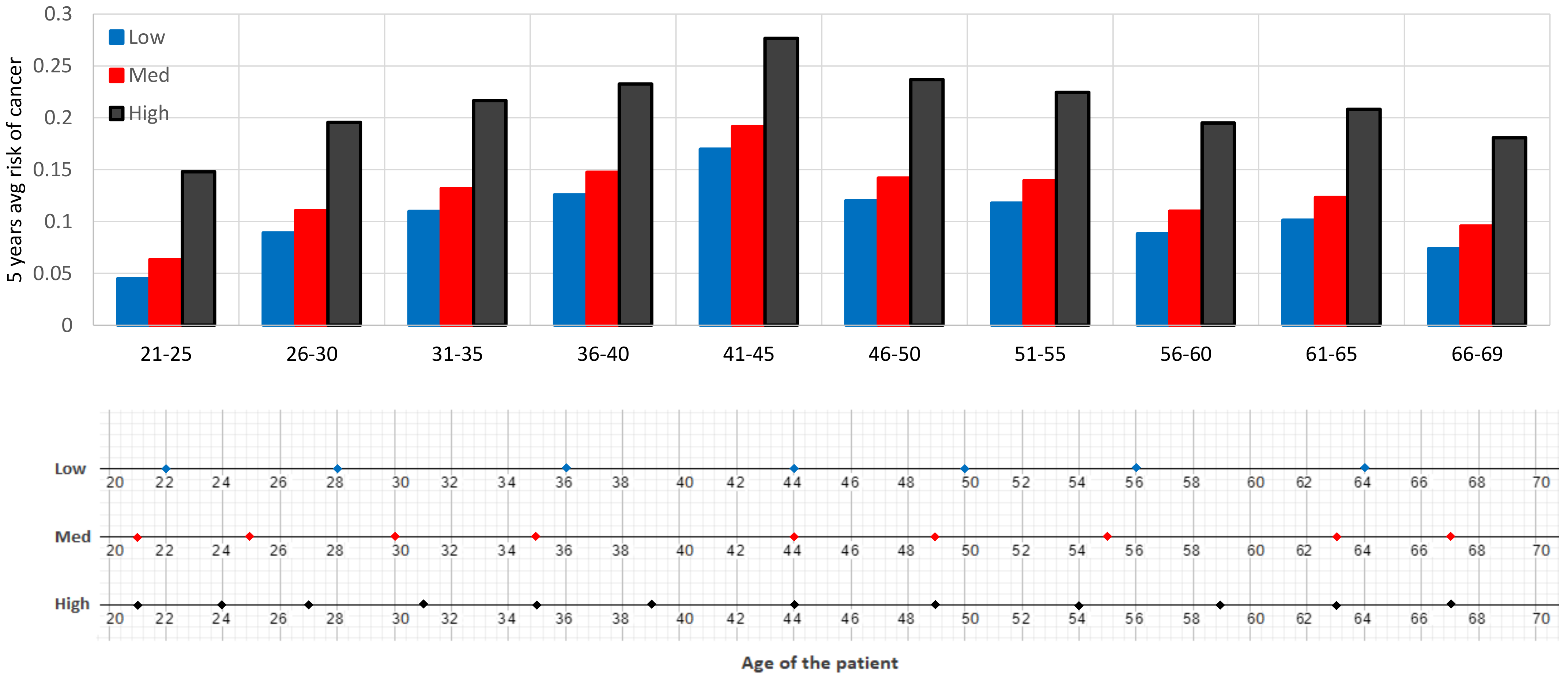
3.1. Optimal Belief-Based Screening Policy

We begin with an example that helps to illustrate how the optimal policy is generated for any patient. Suppose a patient at age 21 with b 0 = [ 0.99 , 0.0071 , 0.0029 ] , meaning that she has a 0.71 % chance of being in state 2 and 0.29 % chance of being in state 3. Based on her age and risk profile, she is expected to undergo screening at age 21. Determining the sequence of following actions throughout the patient’s lifetime requires the knowledge of the current and subsequent action’s outcome. If the test result is negative, b 0 is accordingly updated with ( a , θ ) = ( C T , C T ) . The output b 1 is then multiplied by each alpha vector in the set of alpha vectors of t = 1 created using the procedure explained in Algorithm 1 of Section 2. This procedure is repeated for every t until the terminal decision epoch.
Under the POMDP policy, for a patient whose belief state at age 21 is b 0 = [ 0.99 , 0.0071 , 0.0029 ] , nine screenings with cotesting are recommended throughout her lifetime at ages 21, 25, 30, 35, 44, 49, 55, 63 and 67.
Patients who start late to screen are exposed to higher risks of lifetime cancer. According to Table 1, a perfectly healthy patient with belief state b 0 = [ 1 , 0 , 0 ] at age 21 who has no history of screening ends with an increased risk of developing infections or lesions. Waiting until age 41 leads to the belief state b 20 = [ 0.714 , 0.251 , 0.035 ] .
Generating the optimal policy for a patient who was perfectly healthy at age 21, but has not undergone any screening until age 41, is similar to those starting at age 21 with the only difference that the initial belief state of the patient at age 41 would be equal to b 20 = [ 0.714 , 0.251 , 0.035 ] . According to our POMDP policy, screening for such a patient involves six cotestings. That is only one less than the screening frequency for a low risk patient who starts screening at age 21.
High risk of cancer is not solely correlated with a late start of screening rounds. Sexually active young patients are also subject to higher risks of new or persistent infections. In this part, we aim to evaluate the impact of the patient’s initial risk profile on the optimal screening policy. We consider three patients starting at age 21 with distinct risk profiles, i.e., low risk, medium risk and high risk. Their initial belief vectors are as follows:
  • Low risk patient: b 0 = [ 0.995 , 0.0029 , 0.0021 ] ,
  • Medium risk patient: b 0 = [ 0.99 , 0.0071 , 0.0029 ] ,
  • High risk patient: b 0 = [ 0.75 , 0.2 , 0.05 ] .
One of the risk measures introduced by the medical community of cervical cancer is the risk of being in any of the states of severe cervical dysplasia (in-situ) and invasive cancer, which together are referred to as CIN 3 + risk. In our POMDP model CIN 3 + risk is equivalent to the belief of being in states 2 and 3. We also introduce two additional measures of risk in our study: five-year and lifetime average risk of cancer, which are the arithmetic means of the CIN 3 + risks. Figure 5 illustrates the difference in the 5-year average CIN 3 + risks for three cohorts of patients with low, medium and high risk.
Even though the initial CIN 3 + risk between three groups is considerably different (i.e., 0.005 for low risk, 0.01 for medium risk, and 0.25 for high risk patients), the observed gap in risk is not directly reflected on the number of screenings. That is, 25 times higher risk of cancer for a high risk patient compared to a medium risk patient, leads to only 30 % more screenings. Average re-screen interval length is the longest for low risk patients. This observation can possibly be explained by the higher length of the time which is required for the low risk patients to develop a large enough risk of cancer to enter the screen-required zone. For each patient group, the optimal age of screening is depicted in Figure 5. Our analysis also shows that for the high risk patients, the lifetime average risk of cancer is considerably higher than low risk patients. The impact of the patient’s risk profile on the screening schedule and the lifetime average risk of cancer is summarized in Table 2.

3.2. Comparison of Multiple Policies and Guidelines

To evaluate the performance of our POMDP model, we compare its resulting optimal policy with a set of static policies or guidelines.
No screening: The base case for our comparison is a patient with the same risk of cancer as given in Section 3 who has performed no screening tests during her lifetime and all of the actions are assumed to be a W action. We call this no screening policy.
Modified US practice: represents a policy that recommends screening with cotesting every five years. Screenings start at the age of 21 and end at age 65. We have modified the US guidelines to make them comparable with our cotesting action, since they start with cytology at age 21, repeating every three years until 30, and shifting to cotesting until age 65 with cotesting repeated every 5 years.
Aggressive plan: In order to show that the policies with more frequent screening do not necessarily improve the QALY, we define a screening policy called aggressive plan. Under this plan, a patient is screened first at age 21 and repeats screening every three years until age 66.
Alternative policy 1: In order to study the effect of age at which screenings are conducted, we defined a static policy with the same number of screenings as suggested by our optimal POMDP policy (i.e., nine screenings throughout the lifetime), but distributed at equal intervals.
Alternative policy 2, and Alternative policy 3: Closely related to the real-world scenarios in which patients start late to undergo screening, we defined two static policies under which patients wait until age 41 and 51, respectively, to begin screening. Under Alternative policy 2, the patient starts screening at age 41 as her first screening round and continues screening every 5 years until age 66. Under Alternative policy 3, the patient starts screening at age 51 as her first screening round and continues screening every 5 years until age 66. Such patients carry a higher risk of remaining undetected. Hence, their lifetime risk of cancer might be higher than those who start early.
In the following part, the focus of the comparison analysis will be on both the expected QALY gains under the POMDP policy with other practices and on the lifetime risk of developing cancer under the POMDP policy with those of the other static policies.

3.2.1. QALY-Based Policy Comparison

To maximize the expected QALY gains throughout the patient’s lifetime, the POMDP policy chooses optimal actions at every age of the patient. The sequence of such actions for a specific patient is discussed in Section 3.1. Under no screening, assuming that such a patient survives until age 70, we observe that the expected QALY gain will be 56.346 , whereas the POMDP policy creates 57.228 QALY gains, an approximate 1.57 % increase relative to the no screening policy. We also observe that Alternative policy 1 creates 57.05 QALYs and is outperformed by POMDP policy. Aggressive plan with the highest screening frequency, creates 57.156 QALYs, lower than that of POMDP policy. Table 3 presents the expected QALY gain under various policies for a 21 years old patient.

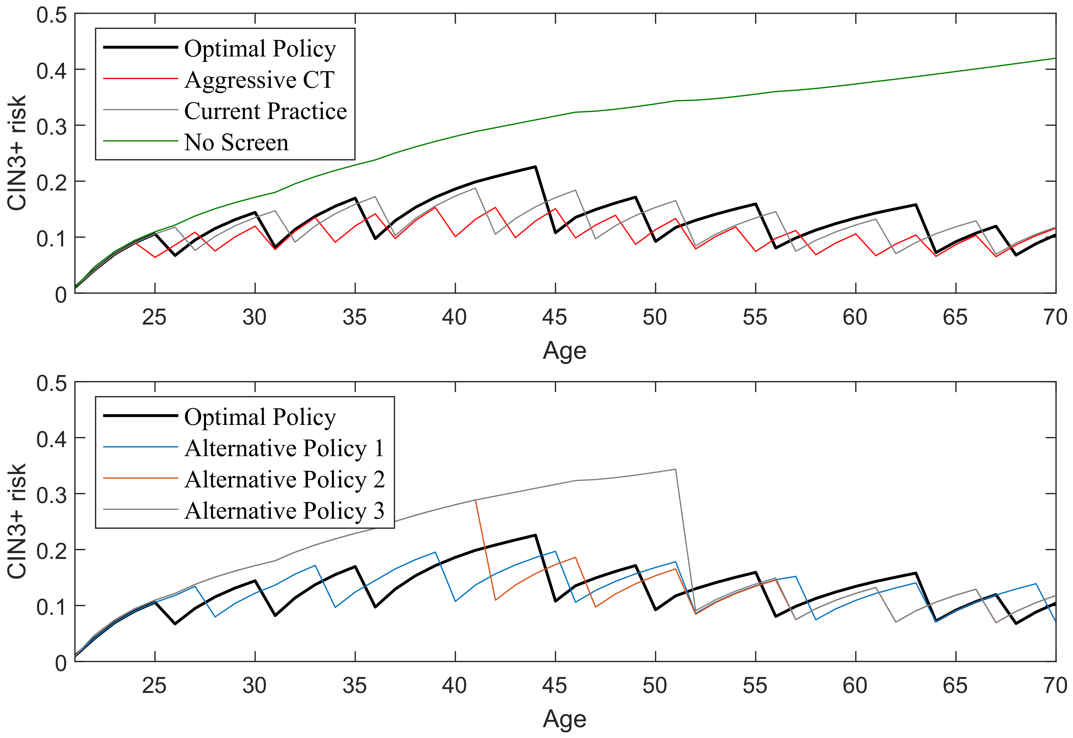
3.2.2. Comparison of Lifetime Cancer Risk across Different Policies

The POMDP model can also be used to study the risks associated with the current guidelines or benchmark practices. Figure 6 illustrates the risk performance of different policies considered. As expected, the risk of doing nothing and waiting is outranking all the other policies. Therefore, Alternative policy 2 and Alternative policy 3 accrue a higher risk until age 40 and 50, respectively, which start to decline as soon as the screening begins. Compared to the other policies, including our POMDP policy, Alternative policy 2 and Alternative policy 3 behave similar to no screening and carry a significantly higher risk until the first screening round. Moreover, one can conclude that Alternative policy 2 exposes the patient to a lower lifetime cancer risk compared to Alternative policy 3 as it is observed in Figure 6, yet there is not much risk difference between Alternative policy 2 and Alternative policy 3 after age 52 until 70. In fact, two patients with the same initial risk, one following Alternative policy 2 and the other following Alternative policy 3 end up at age 70 with the same risk even though in the latter case the patient starts screening 10 years later.

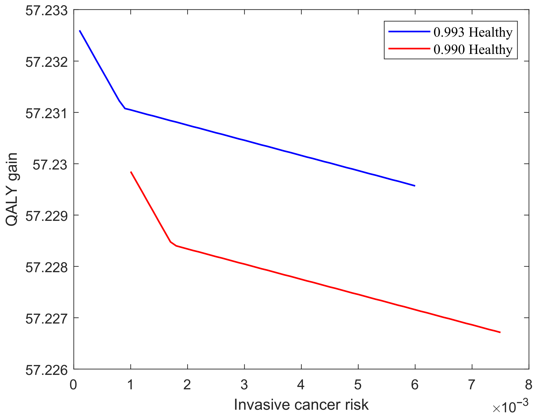
3.3. Sensitivity Analysis

In this section we analyze the model’s behavior with respect to different initial belief states. In other words, this study aims to investigate how our personalized POMDP model behaves while varying the initial belief. This can be interpreted as follows: For a pool of patients at age 21 with different initial cancer risk, what will be the life expectancy? To answer this question, we are looking at two sets of initial belief points.
  • Set 1: high risk patients who are 99 % healthy and their invasive cancer risks vary between 0.25 % and 0.90 % . This case is shown with a red line in Figure 7.
  • Set 2: medium risk patients who are 99.3 % healthy and their invasive cancer risks vary between 0.05 % and 0.70 % . This case is shown with a blue line in Figure 7.
As it is shown in Figure 7, one intuitive interpretation is that healthier patients are expected to gain more life expectancy under the POMDP model. For the patients in Set 1, the higher the risk of invasive cancer, the lower the expected QALY gain. The sudden drop in both graphs can be attributed to the age factor in QALY gain. That is, younger patients on average are gaining more life expectancy up to a certain age.

4. Discussion

“One size fits all” screening guidelines have recently been challenged by the newly introduced personalized screenings. In this study, using a POMDP approach, we developed a personalized screening policy for cervical cancer, which stratifies risk and generates a policy to follow. We showed that our proposed POMDP policy compared to the guidelines, in addition to being more patient representative, improves the life expectancy of the patients. The objective function of our POMDP model maximizes the quality adjusted life years (QALY), which indirectly includes the lifetime risk of cancer as part of the life-quality of the patient. Excessive testing increases the chance of false positive results, which in turn reduces the life quality of the patient due to unnecessary follow ups. By maximizing QALY, we simultaneously reward the lifetime cancer risk reduction and penalize the impact of false positive results. Therefore, the proposed policy by our POMDP model balances the benefits of the testing and the disutility of excessive testing and hence, results in a slightly higher lifetime cancer risk but increasing the overall life-quality of the patient.
Early screening and detection is critical to reducing the future cancer risk of the patients. As we show by one instance, starting screening at the age of 21 versus 41 can relatively reduce the cancer risk while applying only one extra screening on the patient in her lifetime. This highlights the impact of starting screening at an early age on the healthcare system both in terms of effectiveness and costs. Our analysis of the impact of the patient’s risk profiles on the screening frequency and the five-year average risk of cancer shows that the screening frequencies are not proportionate to the cancer risk.
One of the important observations made from our result is the lower QALY gain of aggressive plans compared to the POMDP policy. Therefore, we can safely conclude that performing more frequent screening does not necessarily lead to higher total QALY gains. Such policies, besides being more costly, could be less reliable too. Reliability of a policy is reduced when the policy results in a higher number of false results. False results of the tests, namely false negative and false positive results are crucial factors to consider while studying the performance of a specific policy and they can be considered as the secondary performance measures. Our results suggest that even though aggressive screening practices result in QALY close to that of the POMDP model, this is achieved with the increase of false test results compared to the POMDP policy.
Our analysis of lifetime risk exhibits that even though no policy is dominant in reducing the lifetime risk, it is clear that the POMDP policy has a slightly higher risk, which can be explained by the lower number of screening tests compared to most of the practices considered. We observe that, as the screening interval gets longer, the risk increases. Therefore, policies with longer screening intervals including the POMDP policy create higher risks. Another important observation made in risk analysis is that the policies that start their first screening later, end in relatively similar risk when the patient reaches age 70. This is due to the fact that a test with negative outcome hugely impacts our belief that the patient is healthy in reality.
A major issue that pervades most of the similar studies is the lack of reliable or abundance of conflicting data. Post treatment survival rates for different treatment types, which is common for cervical lesions and cervical cancer, are rarely studied in the literature. It should be noted that an important aspect of the recommendations obtained by a POMDP solution is how accurately a generated belief state represents the state of the patient. In this regard, an important limitation of this study is the lack of a risk estimation module similar to the Framingham Risk Score for cardiovascular disease or the Gail model for breast cancer.
Future research will consider the problem of a generative model for belief states, which receives two types of inputs: the disease attributes and biomarkers specific to HPV and cervical carcinoma, which altogether shape the body of knowledge of the decision maker. Identifying pertinent biomarkers requires the assistance of a cytopathologist, which will render a more reliable belief state if such information is supplied to the generative model. The second type relates to the patient attributes. The more such attributes are included, the more precise the belief estimates will be. In addition, by taking over the role of the Bayesian belief update approach, the generative model approach can remove the dependency on a pure probabilistic update procedure.

Author Contributions

Conceptualization, M.E.; Data curation, M.E.; Formal analysis, M.E. and R.A.-T.; Investigation, M.E.; Methodology, M.E. and R.A.-T.; Supervision, R.A.-T.; Validation, M.E.; Visualization, M.E.; Writing—original draft, M.E. and R.A.-T.; Writing—review and editing, M.E. and R.A.-T. All authors have read and agreed to the published version of the manuscript.

Funding

This research received no external funding.

Institutional Review Board Statement

Not applicable.

Informed Consent Statement

Not applicable.

Data Availability Statement

Data sharing not applicable. No new data were created or analyzed in this study. Data sharing is not applicable to this article.

Conflicts of Interest

The authors declare no conflict of interest.

Appendix A. Data Sources and Data Collection

The primary source of inputs in our model is the literature of cervical cancer, which is summarized in Table A1.
Table A1. Source of model parameters.
ParameterSource
State transitionsJC et al. [75], Campos et al. [76]
Sensitivity and specificity of cotestingJC et al. [75]
Probability of cancerous deathJC et al. [75]
Probability of noncancer deathMcLay et al. [77]
Disutility of BiopsyVelanovich Velanovich [78], Hanmer et al. [79]
Survival ratesSEER data [80]
Life expectancySEER data [80]
Quality of lifeUS life tables [81]
Based on the method explained in Arias and Xu [81] and the US life tables, we use the following terminating rewards in our calculations; r T ( 1 ) = 11 , r T ( 2 ) = 11 , r T ( 3 ) = 9.75 , r T ( 4 ) = 10 , r T ( 5 ) = 10 , r T ( 6 ) = 0 . The method estimates the age-specific life expectancy based on the current state and mortality rate. According to the table, the life expectancy of a patient at age 69 who is in state 1 is 11 years. For the cotesting action, we use the following scores as the disutility in our model. One day for a negative test result, two weeks for a true positive test result and four weeks for a false-positive test result. We assume the initial disutility of doing biopsy is 2 weeks [50], which is increasing over time, meaning that disutility of biopsy for older patients is higher. This is mainly due to the increased risk of adverse side effects of biopsy in older ages. We assume that the disutility associated with biopsy is inversely proportional to the age-specific EQ-5D scores, a utility-based measure of health status widely used in clinical and economic evaluation of health care. These scores reflect varying negative impacts of biopsy on women’s health at different ages. We use the estimates of Hammer et al. [79]. Table A2 summarizes the age-specific EQ-5D scores and our estimates of disutility of biopsy.
Similar to the approach proposed by Ayer et al. [28], we use the age-specific post cancer mortality rates from SEER data and apply the method described in Arias [81] to calculate these rewards. The mortality rate data in SEER is reported based on the cancer stage of localized, regional and distant. According to our definition of states in our Markov chain, those stages are part of our cancer state 3. Hence, we combine all those stages into one stage. Table A3 summarizes the data related to the test characteristics used in our model.
Table A2. Age dependent disutility of biopsy.
Age Group20–2930–3940–4950–5960–6970–7980–89
EQ-5D values0.9130.8930.8630.8370.8110.7710.724
Disutility of biopsy (weeks)22.042.122.182.252.372.52
Table A3. Data related to test characteristics and observation probabilities.
AgeSens(CT,2)Sens(CT,3)Specificity CIN3+ Threshold k CT ( CT | s ) k CT ( CT + | s )
States
123 123
21–690.6250.9910.991 0.9910.3750.009 0.0090.6250.991

References

  1. Arbyn, M.; Weiderpass, E.; Bruni, L.; de Sanjosé, S.; Saraiya, M.; Ferlay, J.; Bray, F. Estimates of incidence and mortality of cervical cancer in 2018: A worldwide analysis. Lancet Glob. Health 2020, 8, e191–e203. [Google Scholar] [CrossRef] [Green Version]
  2. Cohen, P.A.; Jhingran, A.; Oaknin, A.; Denny, L. Cervical cancer. Lancet 2019, 393, 169–182. [Google Scholar] [CrossRef]
  3. Walboomers, J.M.; Jacobs, M.V.; Manos, M.M.; Bosch, F.X.; Kummer, J.A.; Shah, K.V.; Snijders, P.J.; Peto, J.; Meijer, C.J.; Muñoz, N. Human papillomavirus is a necessary cause of invasive cervical cancer worldwide. J. Pathol. 1999, 189, 12–19. [Google Scholar] [CrossRef]
  4. Wilson, K.L.; Cowart, C.J.; Rosen, B.L.; Pulczinski, J.C.; Solari, K.D.; Ory, M.G.; Smith, M.L. Characteristics associated with HPV diagnosis and perceived risk for cervical cancer among unmarried, sexually active college women. J. Cancer Educ. 2018, 33, 404–416. [Google Scholar] [CrossRef] [PubMed]
  5. Jones, J.; Saleem, A.; Rai, N.; Shylasree, T.; Ashman, S.; Gregory, K.; Powell, N.; Tristram, A.; Fiander, A.; Hibbitts, S. Human Papillomavirus genotype testing combined with cytology as a ‘test of cure’post treatment: The importance of a persistent viral infection. J. Clin. Virol. 2011, 52, 88–92. [Google Scholar] [CrossRef]
  6. Alizon, S.; Murall, C.; Bravo, I. Why human papillomavirus acute infections matter. Viruses 2017, 9, 293. [Google Scholar] [CrossRef] [PubMed]
  7. Bennett, K.F.; Waller, J.; Chorley, A.J.; Ferrer, R.A.; Haddrell, J.B.; Marlow, L.A. Barriers to cervical screening and interest in self-sampling among women who actively decline screening. J. Med. Screen. 2018, 25, 211–217. [Google Scholar] [CrossRef]
  8. Silkensen, S.L.; Schiffman, M.; Sahasrabuddhe, V.; Flanigan, J.S. Is It Time to Move Beyond Visual Inspection with Acetic Acid for Cervical Cancer Screening? Glob Health Sci Pract. 2018, 6, 242–246. [Google Scholar] [CrossRef] [PubMed] [Green Version]
  9. Kessler, T.A. Cervical cancer: Prevention and early detection. In Seminars in Oncology Nursing; Elsevier: Amsterdam, The Netherlands, 2017; Volume 33, pp. 172–183. [Google Scholar]
  10. Castle, P.E.; de Sanjosé, S.; Qiao, Y.L.; Belinson, J.L.; Lazcano-Ponce, E.; Kinney, W. Introduction of human papillomavirus DNA screening in the world: 15 years of experience. Vaccine 2012, 30, F117–F122. [Google Scholar] [CrossRef]
  11. Schiffman, M.; Kinney, W.K.; Cheung, L.C.; Gage, J.C.; Fetterman, B.; Poitras, N.E.; Lorey, T.S.; Wentzensen, N.; Befano, B.; Schussler, J.; et al. Relative performance of HPV and cytology components of cotesting in cervical screening. JNCI J. Natl. Cancer Inst. 2017, 110, 501–508. [Google Scholar] [CrossRef]
  12. Polman, N.; Snijders, P.; Kenter, G.; Berkhof, J.; Meijer, C. HPV-based cervical screening: Rationale, expectations and future perspectives of the new Dutch screening programme. Prev. Med. 2018, 119, 108–117. [Google Scholar] [CrossRef]
  13. Aref-Adib, M.; Freeman-Wang, T. Cervical cancer prevention and screening: The role of human papillomavirus testing. Obstet. Gynaecol. 2016, 18, 251–263. [Google Scholar] [CrossRef] [Green Version]
  14. Hartmann, K.; Hall, S.; Nanda, K. Systematic evidence review number 25: Screening for cervical cancer. In Rockville, MD: US Department of Health and Human Services; CreateSpace Independent Publishing Platform: Scotts Valley, CA, USA, 2016. [Google Scholar]
  15. Stumbar, S.E.; Stevens, M.; Feld, Z. Cervical cancer and its precursors: A preventative approach to screening, diagnosis, and management. Prim. Care Clin. Off. Pract. 2019, 46, 117–134. [Google Scholar] [CrossRef] [PubMed]
  16. Johnson, C.A.; James, D.; Marzan, A.; Armaos, M. Cervical cancer: An overview of pathophysiology and management. In Seminars in Oncology Nursing; Elsevier: Amsterdam, The Netherlands, 2019; Volume 35, pp. 166–174. [Google Scholar]
  17. Basu, P.; Meheus, F.; Chami, Y.; Hariprasad, R.; Zhao, F.; Sankaranarayanan, R. Management algorithms for cervical cancer screening and precancer treatment for resource-limited settings. Int. J. Gynecol. Obstet. 2017, 138, 26–32. [Google Scholar] [CrossRef] [PubMed] [Green Version]
  18. Dijkstra, M.G.; van Zummeren, M.; Rozendaal, L.; van Kemenade, F.J.; Helmerhorst, T.J.; Snijders, P.J.; Meijer, C.J.; Berkhof, J. Safety of extending screening intervals beyond five years in cervical screening programmes with testing for high risk human papillomavirus: 14 year follow-up of population based randomised cohort in the Netherlands. BMJ 2016, 355, i4924. [Google Scholar] [CrossRef] [PubMed] [Green Version]
  19. Kitchener, H.C.; Gilham, C.; Sargent, A.; Bailey, A.; Albrow, R.; Roberts, C.; Desai, M.; Mather, J.; Turner, A.; Moss, S.; et al. A comparison of HPV DNA testing and liquid based cytology over three rounds of primary cervical screening: Extended follow up in the ARTISTIC trial. Eur. J. Cancer 2011, 47, 864–871. [Google Scholar] [CrossRef]
  20. Wentzensen, N.; Schiffman, M.; Palmer, T.; Arbyn, M. Triage of HPV positive women in cervical cancer screening. J. Clin. Virol. 2016, 76, S49–S55. [Google Scholar] [CrossRef] [PubMed] [Green Version]
  21. Benard, V.B.; Castle, P.E.; Jenison, S.A.; Hunt, W.C.; Kim, J.J.; Cuzick, J.; Lee, J.H.; Du, R.; Robertson, M.; Norville, S.; et al. Population-based incidence rates of cervical intraepithelial neoplasia in the human papillomavirus vaccine era. JAMA Oncol. 2017, 3, 833–837. [Google Scholar] [CrossRef] [Green Version]
  22. Pileggi, C.; Flotta, D.; Bianco, A.; Nobile, C.G.; Pavia, M. Is HPV DNA testing specificity comparable to that of cytological testing in primary cervical cancer screening? Results of a meta-analysis of randomized controlled trials. Int. J. Cancer 2014, 135, 166–177. [Google Scholar] [CrossRef] [PubMed]
  23. Smith, R.A.; Andrews, K.S.; Brooks, D.; Fedewa, S.A.; Manassaram-Baptiste, D.; Saslow, D.; Wender, R.C. Cancer screening in the United States, 2019: A review of current American Cancer Society guidelines and current issues in cancer screening. CA Cancer J. Clin. 2019, 69, 184–210. [Google Scholar] [CrossRef]
  24. Salina Zhang, B.; Batur, P.; Ncmp, C. Human papillomavirus in 2019: An update on cervical cancer prevention and screening guidelines. Clevel. Clin. J. Med. 2019, 86, 173. [Google Scholar] [CrossRef] [Green Version]
  25. Gelband, H.; Sankaranarayanan, R.; Gauvreau, C.L.; Horton, S.; Anderson, B.O.; Bray, F.; Cleary, J.; Dare, A.J.; Denny, L.; Gospodarowicz, M.K.; et al. Costs, affordability, and feasibility of an essential package of cancer control interventions in low-income and middle-income countries: Key messages from Disease Control Priorities. Lancet 2016, 387, 2133–2144. [Google Scholar] [CrossRef] [Green Version]
  26. Silver, M.I.; Rositch, A.F.; Phelan-Emrick, D.F.; Gravitt, P.E. Uptake of HPV testing and extended cervical cancer screening intervals following cytology alone and Pap/HPV cotesting in women aged 30–65 years. Cancer Causes Control 2018, 29, 43–50. [Google Scholar] [CrossRef] [PubMed]
  27. Lees, B.F.; Erickson, B.K.; Huh, W.K. Cervical cancer screening: Evidence behind the guidelines. Am. J. Obstet. Gynecol. 2016, 214, 438–443. [Google Scholar] [CrossRef] [PubMed]
  28. Ayer, T.; Chen, Q. Personalized medicine. In Handbook of Healthcare Analytics: Theoretical Minimum for Conducting 21st Century Research on Healthcare Operations; Wiley: Hoboken, NJ, USA, 2018; pp. 109–135. [Google Scholar]
  29. Wright, T.C.; Stoler, M.H.; Behrens, C.M.; Sharma, A.; Zhang, G.; Wright, T.L. Primary cervical cancer screening with human papillomavirus: End of study results from the ATHENA study using HPV as the first-line screening test. Gynecol. Oncol. 2015, 136, 189–197. [Google Scholar] [CrossRef] [PubMed] [Green Version]
  30. Kinney, W.; Fetterman, B.; Cox, J.T.; Lorey, T.; Flanagan, T.; Castle, P.E. Characteristics of 44 cervical cancers diagnosed following Pap-negative, high risk HPV-positive screening in routine clinical practice. Gynecol. Oncol. 2011, 121, 309–313. [Google Scholar] [CrossRef] [PubMed] [Green Version]
  31. Konecny, G.E. The path to personalized medicine in women’s cancers: Challenges and recent advances. Curr. Opin. Obstet. Gynecol. 2015, 27, 45–47. [Google Scholar] [CrossRef] [Green Version]
  32. Robertson, D.J.; Ladabaum, U. Opportunities and challenges in moving from current guidelines to personalized colorectal cancer screening. Gastroenterology 2019, 156, 904–917. [Google Scholar] [CrossRef] [Green Version]
  33. Güneş, E.D.; Örmeci, E.L. Or applications in disease screening. In Operations Research Applications in Health Care Management; Springer: Berlin/Heidelberg, Germany, 2018; pp. 297–325. [Google Scholar]
  34. Alagoz, O.; Hsu, H.; Schaefer, A.J.; Roberts, M.S. Markov decision processes: A tool for sequential decision making under uncertainty. Med. Decis. Mak. 2010, 30, 474–483. [Google Scholar] [CrossRef] [PubMed]
  35. Steimle, L.N.; Denton, B.T. Markov decision processes for screening and treatment of chronic diseases. In Markov Decision Processes in Practice; Springer: Berlin/Heidelberg, Germany, 2017; pp. 189–222. [Google Scholar]
  36. Chhatwal, J.; Alagoz, O.; Burnside, E.S. Optimal breast biopsy decision-making based on mammographic features and demographic factors. Oper. Res. 2010, 58, 1577–1591. [Google Scholar] [CrossRef]
  37. Alagoz, O.; Chhatwal, J.; Burnside, E.S. Optimal policies for reducing unnecessary follow-up mammography exams in breast cancer diagnosis. Decis. Anal. 2013, 10, 200–224. [Google Scholar] [CrossRef] [Green Version]
  38. Burnside, E.S.; Chhatwal, J.; Alagoz, O. What is the optimal threshold at which to recommend breast biopsy? PLoS ONE 2012, 7, e48820. [Google Scholar]
  39. Yaylali, E.; Karamustafa, U. A Markov Decision Process Approach to Estimate the Risk of Obesity Related Cancers. In Industrial Engineering in the Big Data Era; Springer: Berlin/Heidelberg, Germany, 2019; pp. 489–502. [Google Scholar]
  40. Ayvaci, M.U.; Alagoz, O.; Burnside, E.S. The effect of budgetary restrictions on breast cancer diagnostic decisions. Manuf. Serv. Oper. Manag. 2012, 14, 600–617. [Google Scholar] [CrossRef] [PubMed] [Green Version]
  41. Önen, Z.; Sayin, S.; Gürvit, I.H. Optimal population screening policies for alzheimer’s disease. IISE Trans. Healthc. Syst. Eng. 2019, 9, 14–25. [Google Scholar] [CrossRef]
  42. Goulionis, J.E.; Koutsiumaris, B. Partially observable Markov decision model for the treatment of early Prostate Cancer. Opsearch 2010, 47, 105–117. [Google Scholar] [CrossRef]
  43. Tomer, A.; Nieboer, D.; Roobol, M.J.; Steyerberg, E.W.; Rizopoulos, D. Personalized schedules for surveillance of low-risk prostate cancer patients. Biometrics 2019, 75, 153–162. [Google Scholar] [CrossRef] [PubMed]
  44. Witteveen, A.; Otten, J.W.; Vliegen, I.M.; Siesling, S.; Timmer, J.B.; IJzerman, M.J. Risk-based breast cancer follow-up stratified by age. Cancer Med. 2018, 7, 5291–5298. [Google Scholar] [CrossRef] [PubMed]
  45. Otten, J.W.M.; Witteveen, A.; Vliegen, I.; Siesling, S.; Timmer, J.B.; IJzerman, M.J. Stratified breast cancer follow-up using a partially observable MDP. In Markov Decision Processes in Practice; Springer: Berlin/Heidelberg, Germany, 2017; pp. 223–244. [Google Scholar]
  46. Gan, K.; Scheller-Wolf, A.A.; Tayur, S.R. Personalized Treatment for Opioid Use Disorder. Available online: https://ssrn.com/abstr-act=3389539 (accessed on 16 May 2019).
  47. Ibrahim, R.; Kucukyazici, B.; Verter, V.; Gendreau, M.; Blostein, M. Designing personalized treatment: An application to anticoagulation therapy. Prod. Oper. Manag. 2016, 25, 902–918. [Google Scholar] [CrossRef] [Green Version]
  48. Ayer, T.; Alagoz, O.; Stout, N.K.; Burnside, E.S. Designing a new breast cancer screening program considering adherence. In Proceedings of the INFORMS Annual Meeting, Austin, TX, USA, 7–11 November 2010. [Google Scholar]
  49. Li, J.; Dong, M.; Ren, Y.; Yin, K. How patient compliance impacts the recommendations for colorectal cancer screening. J. Comb. Optim. 2015, 30, 920–937. [Google Scholar] [CrossRef]
  50. Ayer, T.; Alagoz, O.; Stout, N.K. OR Forum—A POMDP approach to personalize mammography screening decisions. Oper. Res. 2012, 60, 1019–1034. [Google Scholar] [CrossRef]
  51. Akhavan-Tabatabaei, R.; Sánchez, D.M.; Yeung, T.G. A Markov decision process model for cervical cancer screening policies in Colombia. Med. Decis. Mak. 2017, 37, 196–211. [Google Scholar] [CrossRef] [PubMed]
  52. Cevik, M.; Ayer, T.; Alagoz, O.; Sprague, B.L. Analysis of mammography screening policies under resource constraints. Prod. Oper. Manag. 2018, 27, 949–972. [Google Scholar] [CrossRef]
  53. Kocken, M.; Helmerhorst, T.J.; Berkhof, J.; Louwers, J.A.; Nobbenhuis, M.A.; Bais, A.G.; Hogewoning, C.J.; Zaal, A.; Verheijen, R.H.; Snijders, P.J.; et al. Risk of recurrent high-grade cervical intraepithelial neoplasia after successful treatment: A long-term multi-cohort study. Lancet Oncol. 2011, 12, 441–450. [Google Scholar] [CrossRef]
  54. Otten, M.; Timmer, J.; Witteveen, A. Stratified breast cancer follow-up using a continuous state partially observable Markov decision process. Eur. J. Oper. Res. 2020, 281, 464–474. [Google Scholar] [CrossRef] [Green Version]
  55. Molani, S.; Madadi, M.; Wilkes, W. A partially observable Markov chain framework to estimate overdiagnosis risk in breast cancer screening: Incorporating uncertainty in patients adherence behaviors. Omega 2019, 89, 40–53. [Google Scholar] [CrossRef]
  56. Leinonen, M.; Nieminen, P.; Kotaniemi-Talonen, L.; Malila, N.; Tarkkanen, J.; Laurila, P.; Anttila, A. Age-specific evaluation of primary human papillomavirus screening vs conventional cytology in a randomized setting. JNCI J. Natl. Cancer Inst. 2009, 101, 1612–1623. [Google Scholar] [CrossRef]
  57. Sonnenberg, F.A.; Beck, J.R. Markov models in medical decision making: A practical guide. Med. Decis. Mak. 1993, 13, 322–338. [Google Scholar] [CrossRef]
  58. Kocken, M.; Uijterwaal, M.H.; de Vries, A.L.; Berkhof, J.; Ket, J.C.; Helmerhorst, T.J.; Meijer, C.J. High-risk human papillomavirus testing versus cytology in predicting post-treatment disease in women treated for high-grade cervical disease: A systematic review and meta-analysis. Gynecol. Oncol. 2012, 125, 500–507. [Google Scholar] [CrossRef] [PubMed]
  59. Hauskrecht, M. Value-function approximations for partially observable Markov decision processes. J. Artif. Intell. Res. 2000, 13, 33–94. [Google Scholar] [CrossRef] [Green Version]
  60. Pineau, J.; Gordon, G.; Thrun, S. Point-based value iteration: An anytime algorithm for POMDPs. IJCAI Citeseer 2003, 3, 1025–1032. [Google Scholar]
  61. Krishnamurthy, V. Structural results for partially observed markov decision processes. arXiv 2015, arXiv:1512.03873. [Google Scholar]
  62. Sondik, E.J. The Optimal Control of Partially Observable Markov Processes; Technical Report; Stanford University California Stanford Electronics Labs: Stanford, CA, USA, 1971. [Google Scholar]
  63. Smallwood, R.D.; Sondik, E.J. The optimal control of partially observable Markov processes over a finite horizon. Oper. Res. 1973, 21, 1071–1088. [Google Scholar] [CrossRef]
  64. Walraven, E.; Spaan, M.T. Point-based value iteration for finite-horizon POMDPs. J. Artif. Intell. Res. 2019, 65, 307–341. [Google Scholar] [CrossRef]
  65. Porta, J.M.; Vlassis, N.; Spaan, M.T.; Poupart, P. Point-Based Value Iteration for Continuous POMDPs. J. Mach. Learn. Res. 2006, 7, 2329–2367. [Google Scholar]
  66. Cassandra, A.R.; Kaelbling, L.P.; Littman, M.L. Acting optimally in partially observable stochastic domains. AAAI 1994, 94, 1023–1028. [Google Scholar]
  67. Monahan, G.E. State of the art—A survey of partially observable Markov decision processes: Theory, models, and algorithms. Manag. Sci. 1982, 28, 1–16. [Google Scholar] [CrossRef] [Green Version]
  68. Cheng, H.T. Algorithms for Partially Observable Markov Decision Processes. Ph.D. Thesis, University of British Columbia, Vancouver, BC, Canada, 1988. [Google Scholar]
  69. Cassandra, A.R.; Littman, M.L.; Zhang, N.L. Incremental pruning: A simple, fast, exact method for partially observable Markov decision processes. arXiv 2013, arXiv:1302.1525. [Google Scholar]
  70. Braziunas, D. POMDP Solution Methods; University of Toronto: Toronto, ON, Canada, 2003. [Google Scholar]
  71. White, C.C. A survey of solution techniques for the partially observed Markov decision process. Ann. Oper. Res. 1991, 32, 215–230. [Google Scholar] [CrossRef] [Green Version]
  72. Raphael, C.; Shani, G. The Skyline algorithm for POMDP value function pruning. Ann. Math. Artif. Intell. 2012, 65, 61–77. [Google Scholar] [CrossRef]
  73. Walraven, E.; Spaan, M. Accelerated vector pruning for optimal POMDP solvers. In Proceedings of the AAAI Conference on Artificial Intelligence, San Francisco, CA, USA, 4–9 February 2017; Volume 31. [Google Scholar]
  74. Eagle, J.N. The optimal search for a moving target when the search path is constrained. Oper. Res. 1984, 32, 1107–1115. [Google Scholar] [CrossRef] [Green Version]
  75. Felix, J.C.; Lacey, M.J.; Miller, J.D.; Lenhart, G.M.; Spitzer, M.; Kulkarni, R. The clinical and economic benefits of co-testing versus primary HPV testing for cervical cancer screening: A modeling analysis. J. Women’s Health 2016, 25, 606–616. [Google Scholar] [CrossRef] [Green Version]
  76. Campos, N.G.; Burger, E.A.; Sy, S.; Sharma, M.; Schiffman, M.; Rodriguez, A.C.; Hildesheim, A.; Herrero, R.; Kim, J.J. An updated natural history model of cervical cancer: Derivation of model parameters. Am. J. Epidemiol. 2014, 180, 545–555. [Google Scholar] [CrossRef] [PubMed]
  77. McLay, L.A.; Foufoulides, C.; Merrick, J.R. Using simulation-optimization to construct screening strategies for cervical cancer. Health Care Manag. Sci. 2010, 13, 294–318. [Google Scholar] [CrossRef] [PubMed]
  78. Velanovich, V. Immediate biopsy versus observation for abnormal findings on mammograms: An analysis of potential outcomes and costs. Am. J. Surg. 1995, 170, 327–332. [Google Scholar] [CrossRef]
  79. Hanmer, J.; Lawrence, W.F.; Anderson, J.P.; Kaplan, R.M.; Fryback, D.G. Report of nationally representative values for the noninstitutionalized US adult population for 7 health-related quality-of-life scores. Med. Decis. Mak. 2006, 26, 391–400. [Google Scholar] [CrossRef] [PubMed]
  80. Siegel, R.L.; Miller, K.D.; Jemal, A. Cancer statistics, 2019. CA Cancer J. Clin. 2019, 69, 7–34. [Google Scholar] [CrossRef] [PubMed] [Green Version]
  81. Arias, E.; Xu, J. Available online: https://www.cdc.gov/nchs/data/nvsr/nvsr68/nvsr68_07-508.pdf (accessed on 24 June 2019).
Figure 1. State transition diagram.
Mathematics 09 00679 g001
Figure 2. Timeline of the decision process.
Mathematics 09 00679 g002
Figure 3. Belief simplex and update of belief states.
Mathematics 09 00679 g003
Figure 4. Alpha vectors over belief space in a two-state partially observable Markov decision process (POMDP); bold segment of the alpha vectors constitute a piecewise linear and convex (PWLC) value function. α 4 is a redundant vector and can be eliminated.
Mathematics 09 00679 g004
Figure 5. Five-year average risk of cancer for patients with different risk profiles. Colored dots show the screening ages of each risk profile.
Mathematics 09 00679 g005
Figure 6. Lifetime risk of cancer under different policies.
Mathematics 09 00679 g006
Figure 7. Quality adjusted life years (QALY) gained under different starting belief points.
Mathematics 09 00679 g007
Table 1. Impact of starting late to screen on the health state of a 41 year old patient who has been healthy at age 21.
Age b t ( 1 ) b t ( 2 ) b t ( 3 )
21100
220.9710.0260.003
230.9440.0500.006
410.7140.2510.035
Table 2. Impact of the patient’s risk profile on the cancer risk and screening schedule.
Risk ProfileLifetime No.
of Screenings
Avg. Screening
Interval Length
Lifetime Avg.
Risk of Cancer
ine Low risk76.860.0849
Medium risk95.330.125
High risk1240.209
Table 3. Comparison of performance across different policies for a 21 year old patient with no test history.
Start
Age
Screen
Interval
Length
Screen
Rounds
Stop
Age
Exp.
False
Results
Exp.
QALY
Gain
Improve
In
QALY(%)
No screening--0-056.346-
Modified US practice21510660.1856.1190
Aggressive plan21316590.25257.1561.4
Alternative policy 12169690.16257.0751.3
Alternative policy 24056660.10857.0041.18
Alternative policy 35054660.07256.8240.87
POMDP policy23variable9670.16257.2281.57
Publisher’s Note: MDPI stays neutral with regard to jurisdictional claims in published maps and institutional affiliations.

