Author Contributions
Conceptualization, J.M. and V.V.; methodology, J.M.; software, E.M.; validation, J.M., M.K., and E.M.; formal analysis, V.V.; investigation, J.M., M.K., and E.M.; resources, V.V.; data curation, J.M.; writing—original draft preparation, J.M., M.K., and E.M.; writing—review and editing, V.V.; visualization, V.V.; supervision, M.K.; project administration, J.M.; funding acquisition, J.M., M.K., V.V., and E.M. All authors have read and agreed to the published version of the manuscript.
Figure 1.
Computational model of vehicle.
Figure 1.
Computational model of vehicle.
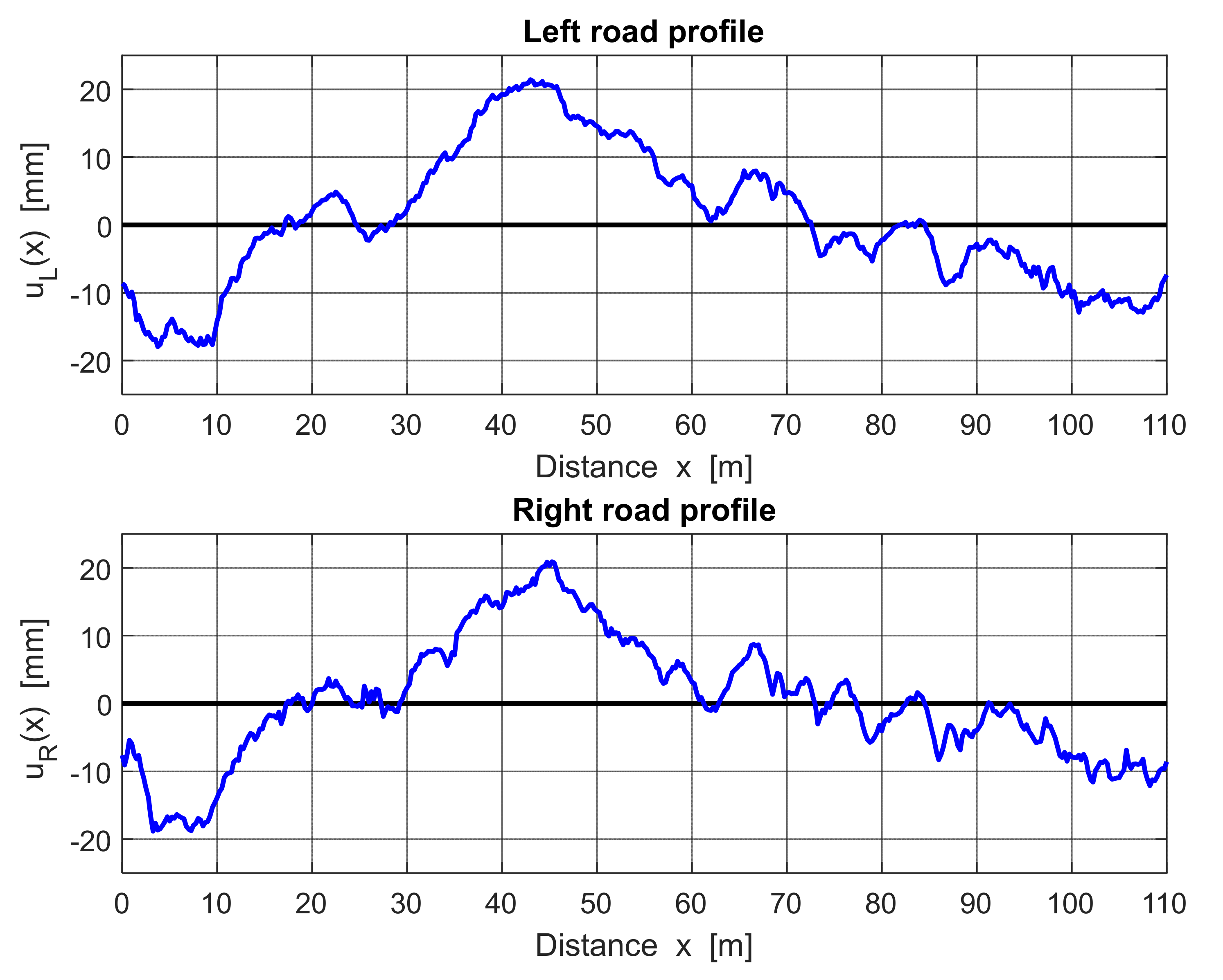
Figure 2.
Left and right road profiles.
Figure 2.
Left and right road profiles.
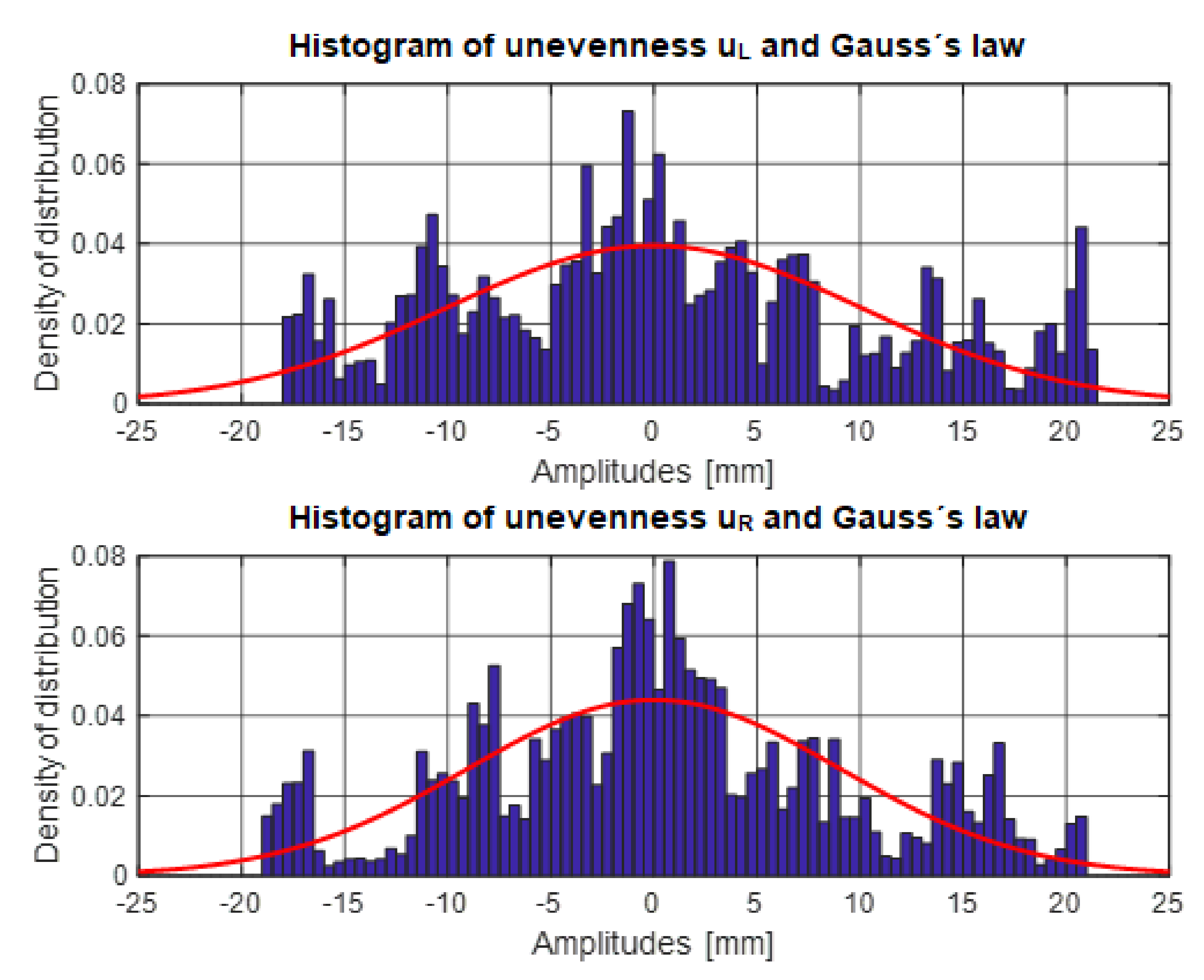
Figure 3.
Histogram of unevenness and Gauss’s law.
Figure 3.
Histogram of unevenness and Gauss’s law.
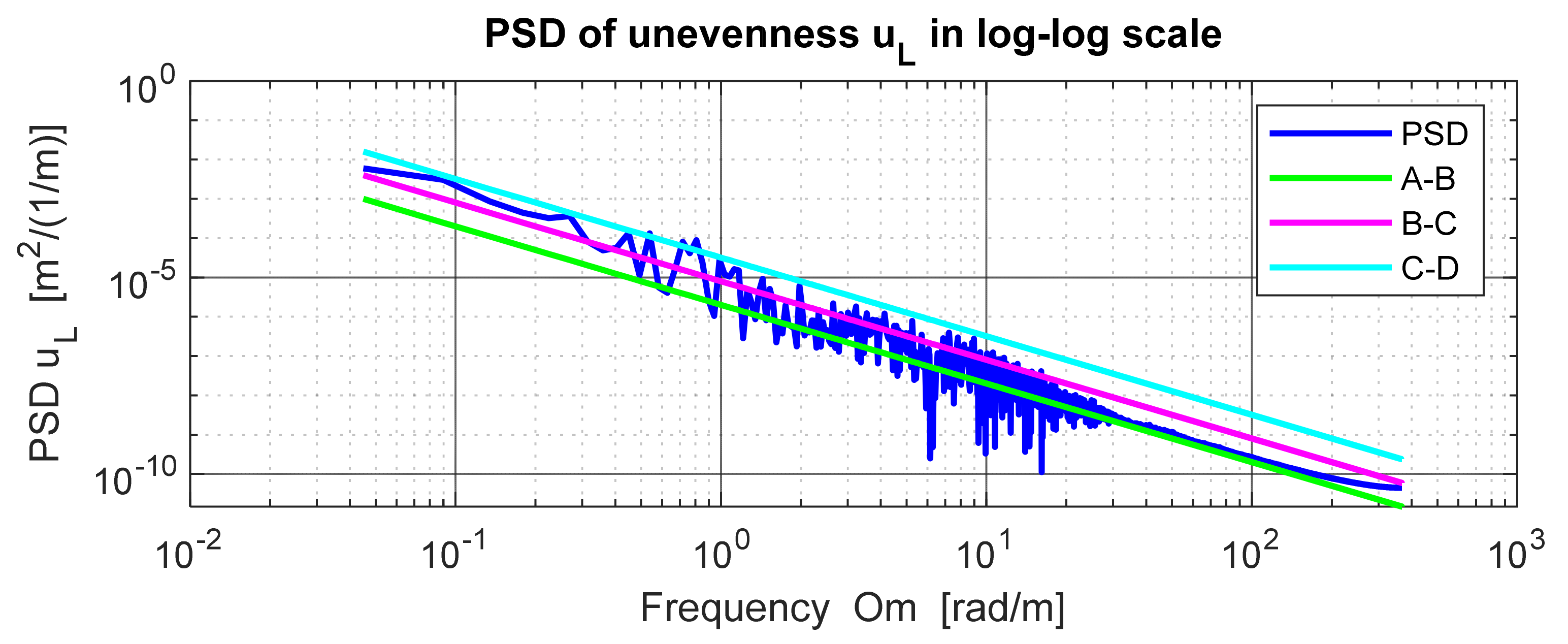
Figure 4.
Power spectral density (PSD) of left road profile in log-log scale.
Figure 4.
Power spectral density (PSD) of left road profile in log-log scale.
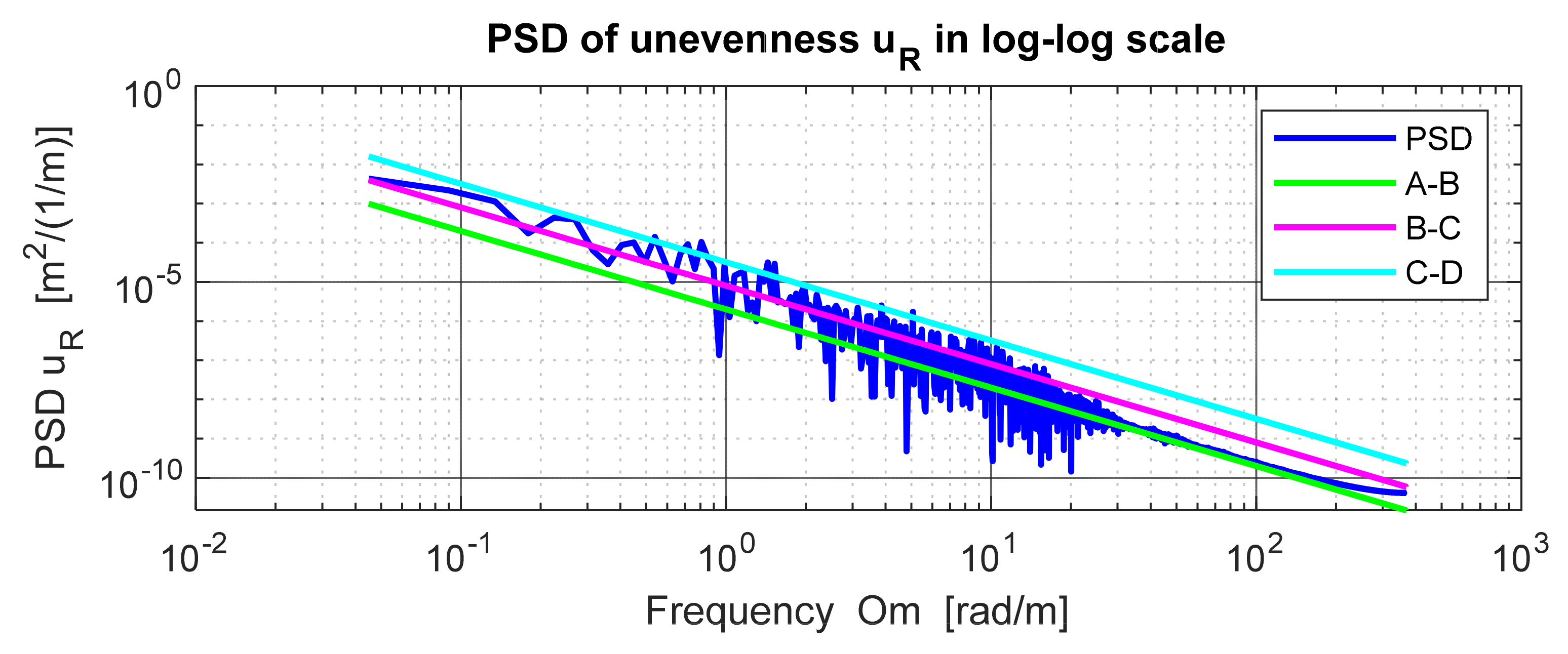
Figure 5.
PSD of right road profile in log-log scale.
Figure 5.
PSD of right road profile in log-log scale.
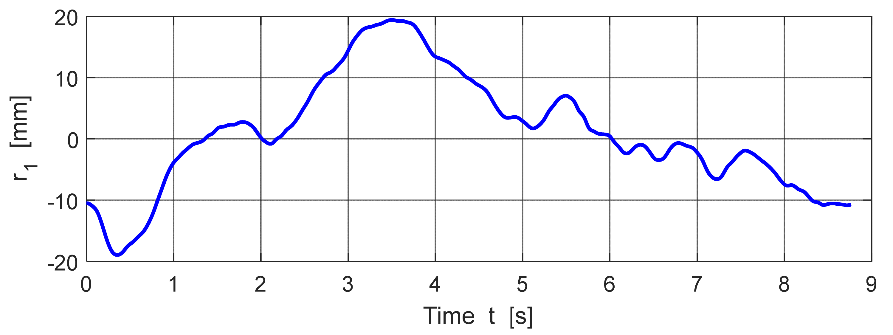
Figure 6.
Vertical deflection of the center of gravity of the sprung mass of vehicle.
Figure 6.
Vertical deflection of the center of gravity of the sprung mass of vehicle.
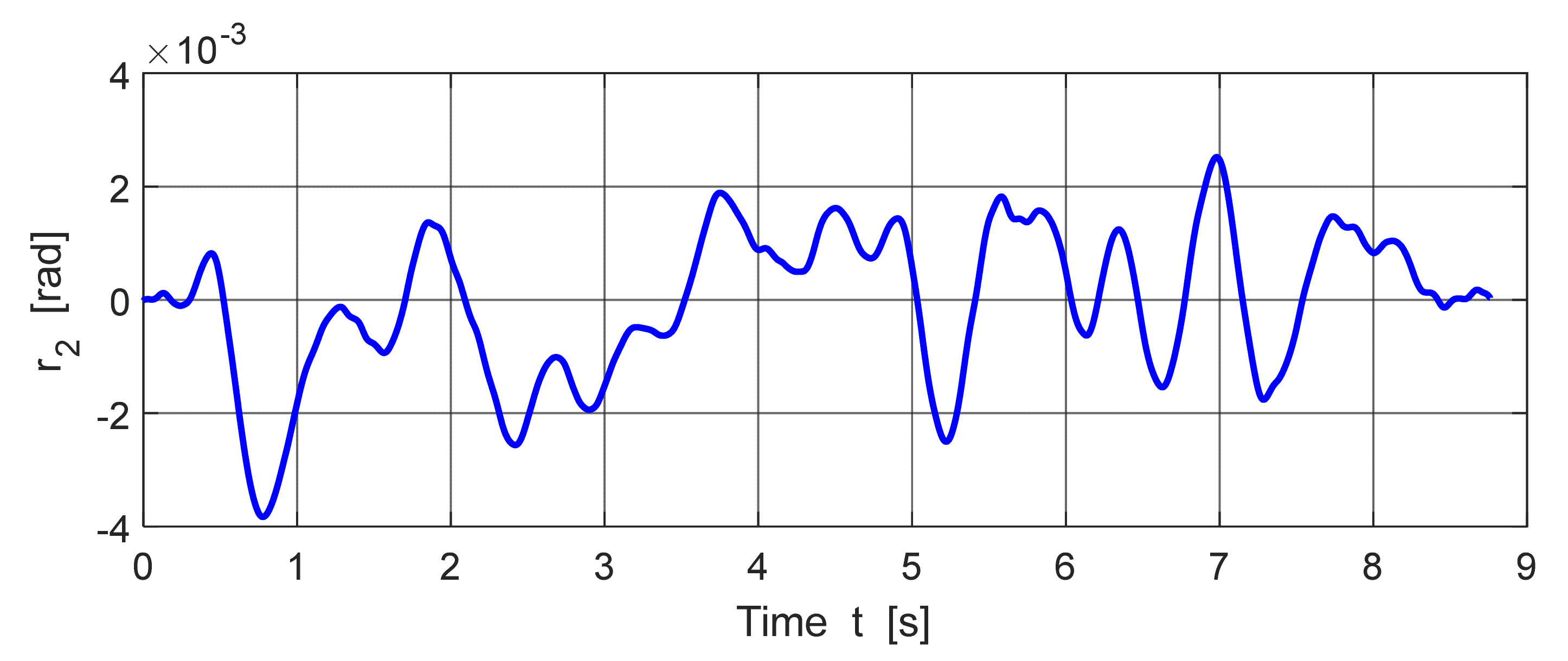
Figure 7.
Angle of rotation of the sprung mass of vehicle in the longitudinal direction about an axis passing through the center of gravity.
Figure 7.
Angle of rotation of the sprung mass of vehicle in the longitudinal direction about an axis passing through the center of gravity.
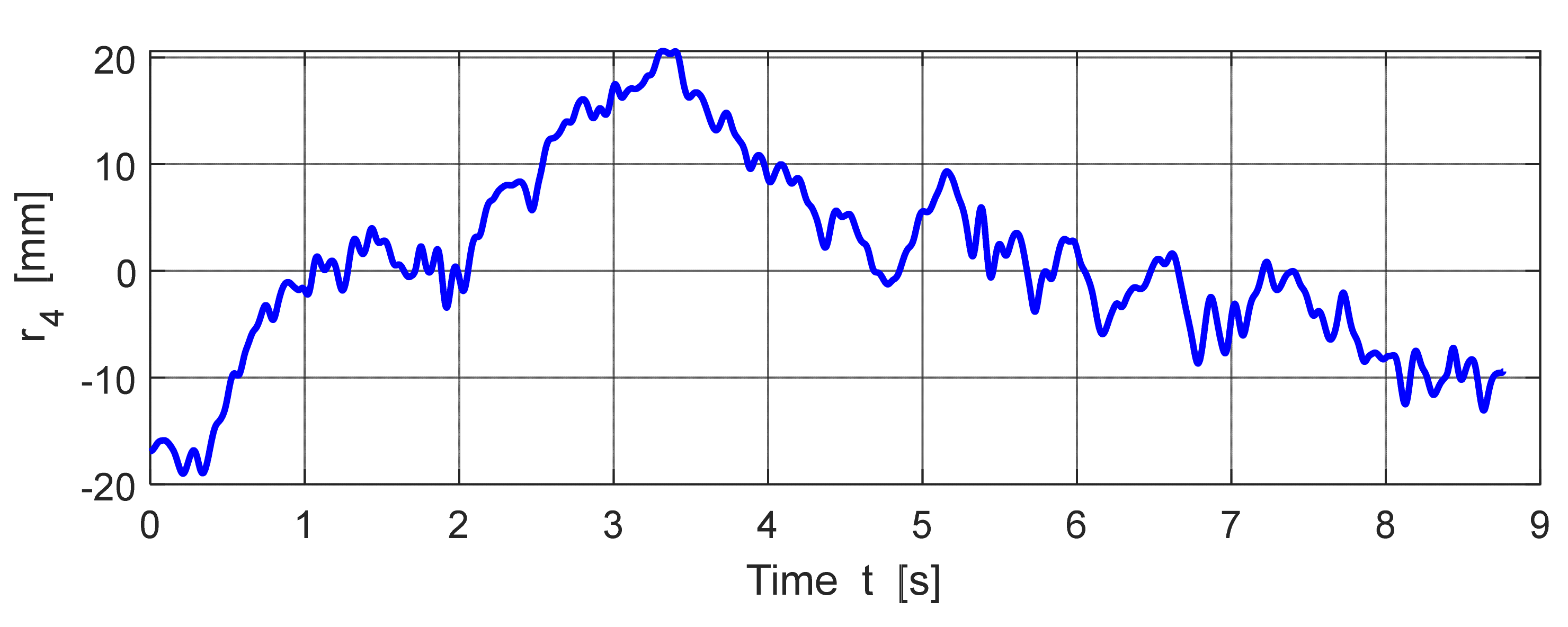
Figure 8.
Vertical deflection of the right front axle of vehicle.
Figure 8.
Vertical deflection of the right front axle of vehicle.
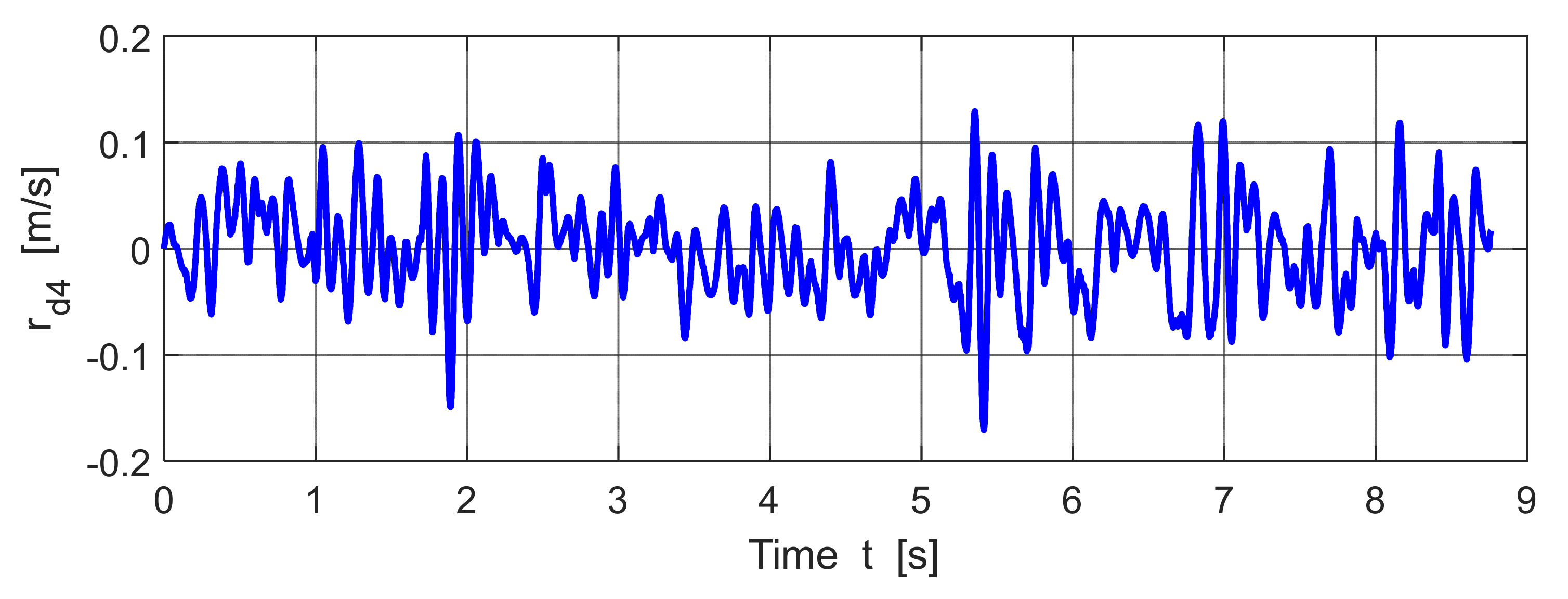
Figure 9.
Speed of vertical motion of the right front axle of vehicle.
Figure 9.
Speed of vertical motion of the right front axle of vehicle.
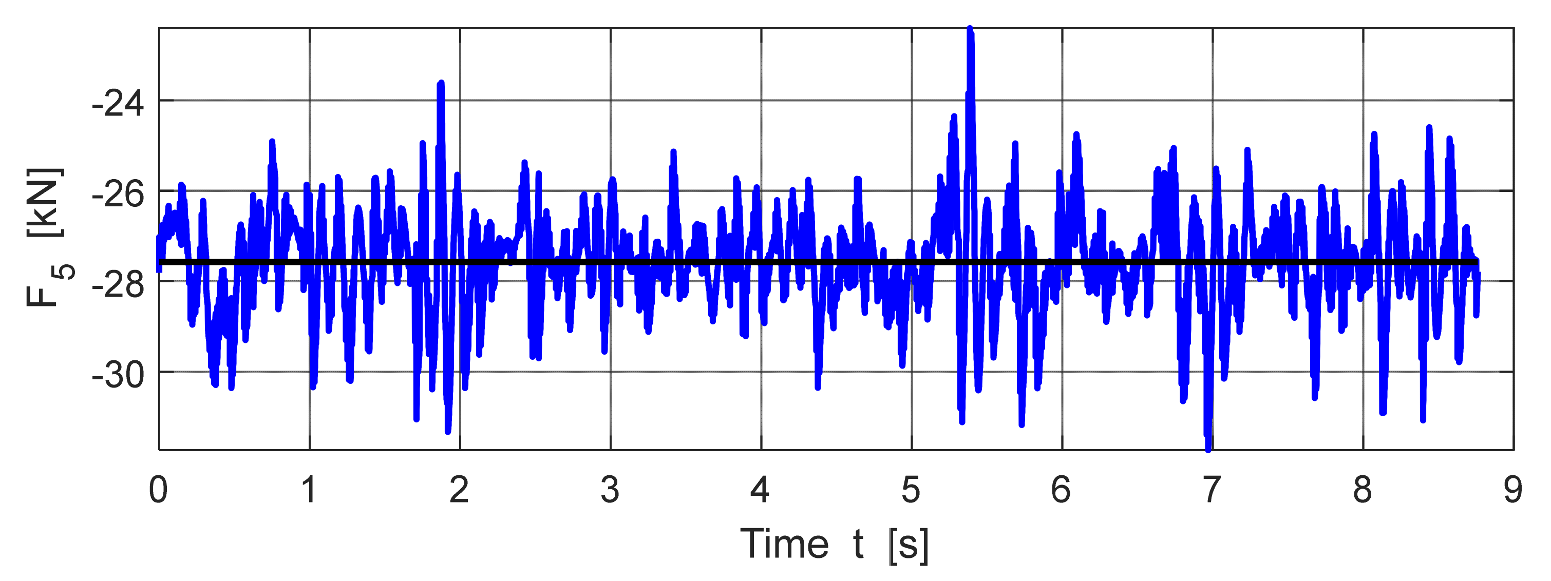
Figure 10.
Contact force between the left rear wheel of the rear axle and the road.
Figure 10.
Contact force between the left rear wheel of the rear axle and the road.
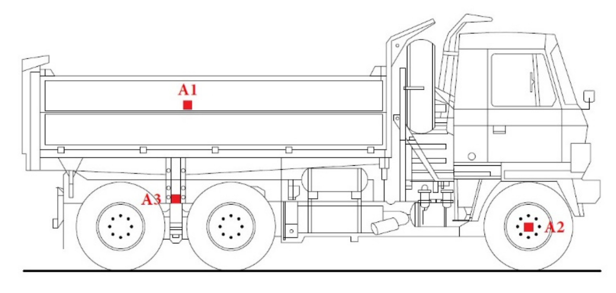
Figure 11.
Localization of sensors on the vehicle.
Figure 11.
Localization of sensors on the vehicle.
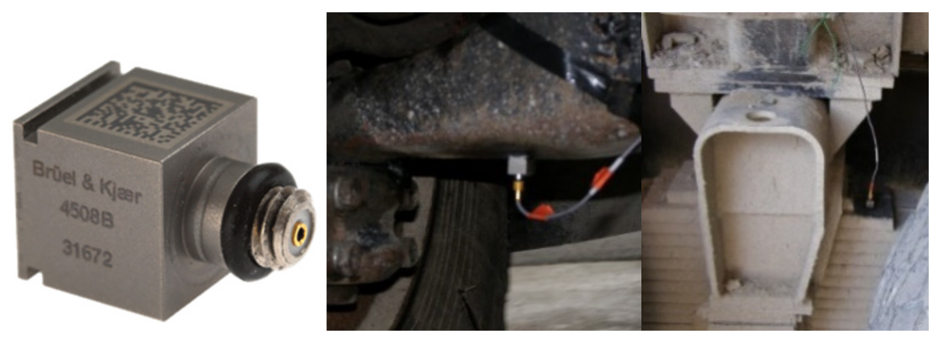
Figure 12.
Sensor and its location on the front and rear axles.
Figure 12.
Sensor and its location on the front and rear axles.
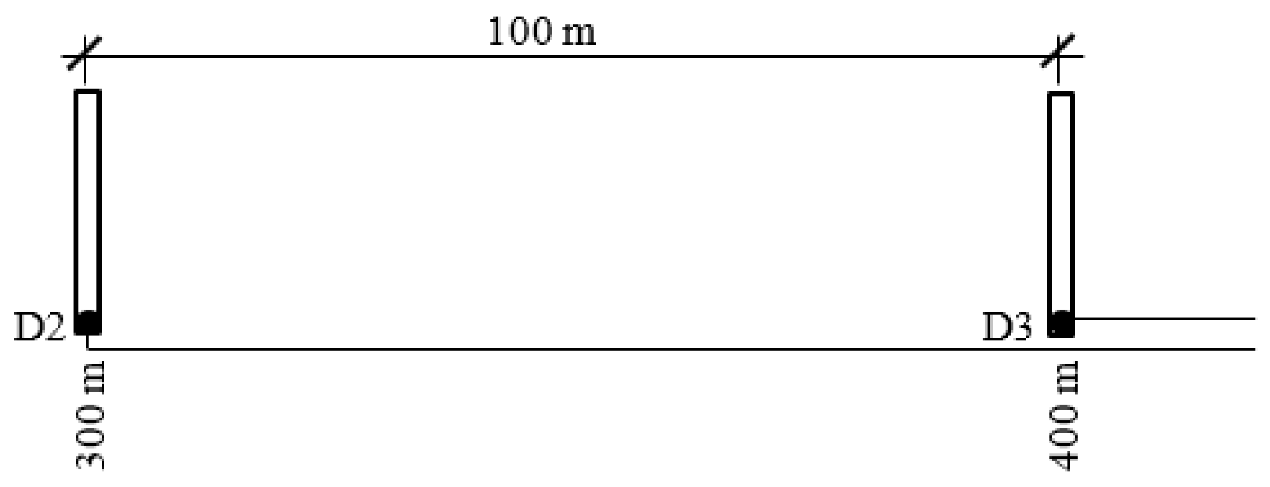
Figure 13.
Steel strips with accelerometers D2 and D3 at a distance of 100 m.
Figure 13.
Steel strips with accelerometers D2 and D3 at a distance of 100 m.
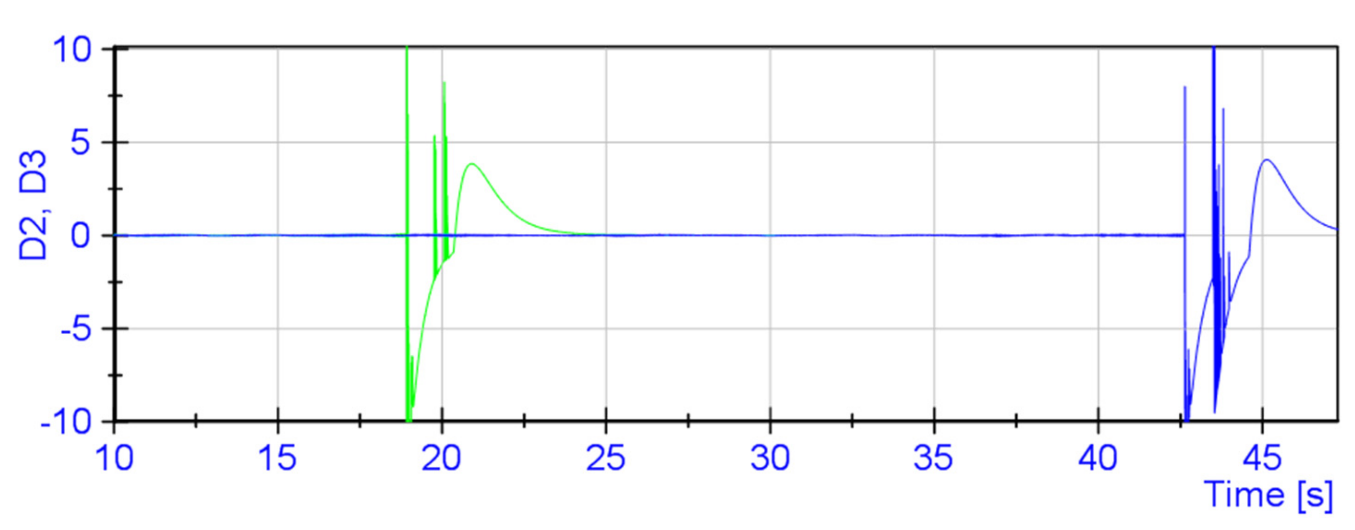
Figure 14.
Records from accelerometers D2 and D3.
Figure 14.
Records from accelerometers D2 and D3.
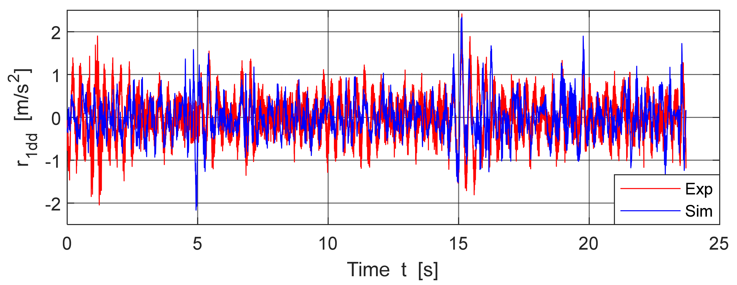
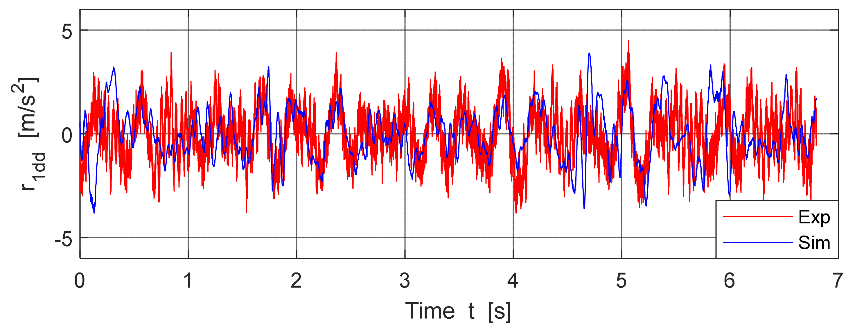
Figure 15.
Acceleration in the center of gravity (CG) of vehicle sprung mass, V = 15.18 km/h.
Figure 15.
Acceleration in the center of gravity (CG) of vehicle sprung mass, V = 15.18 km/h.
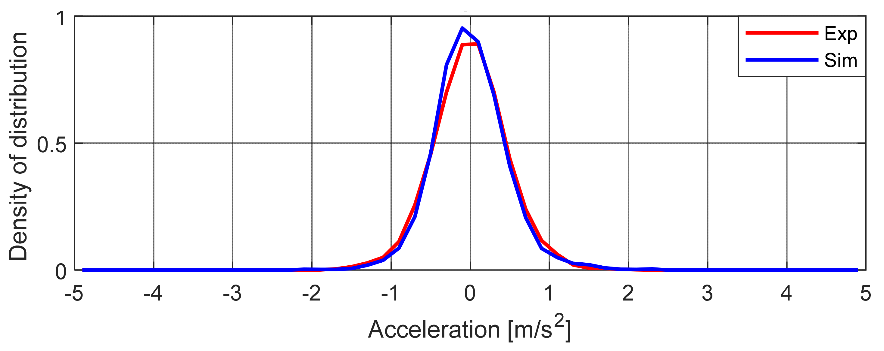
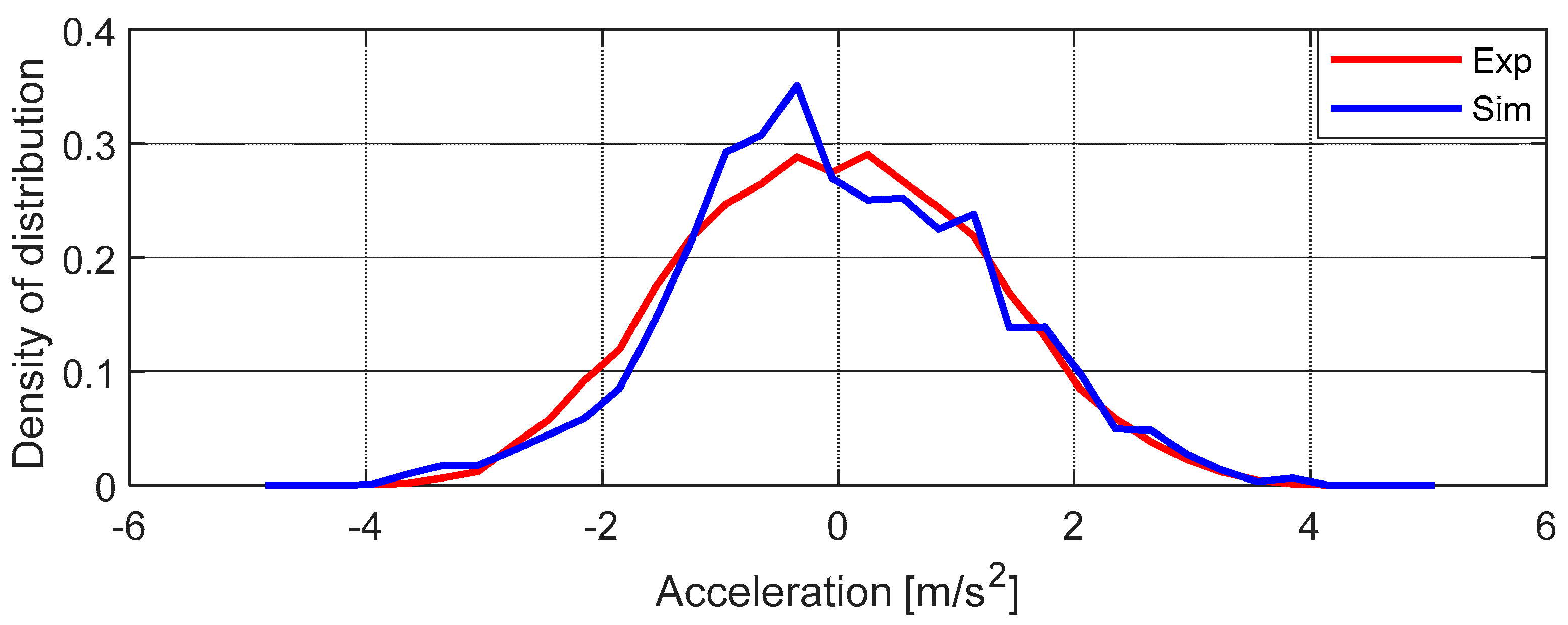
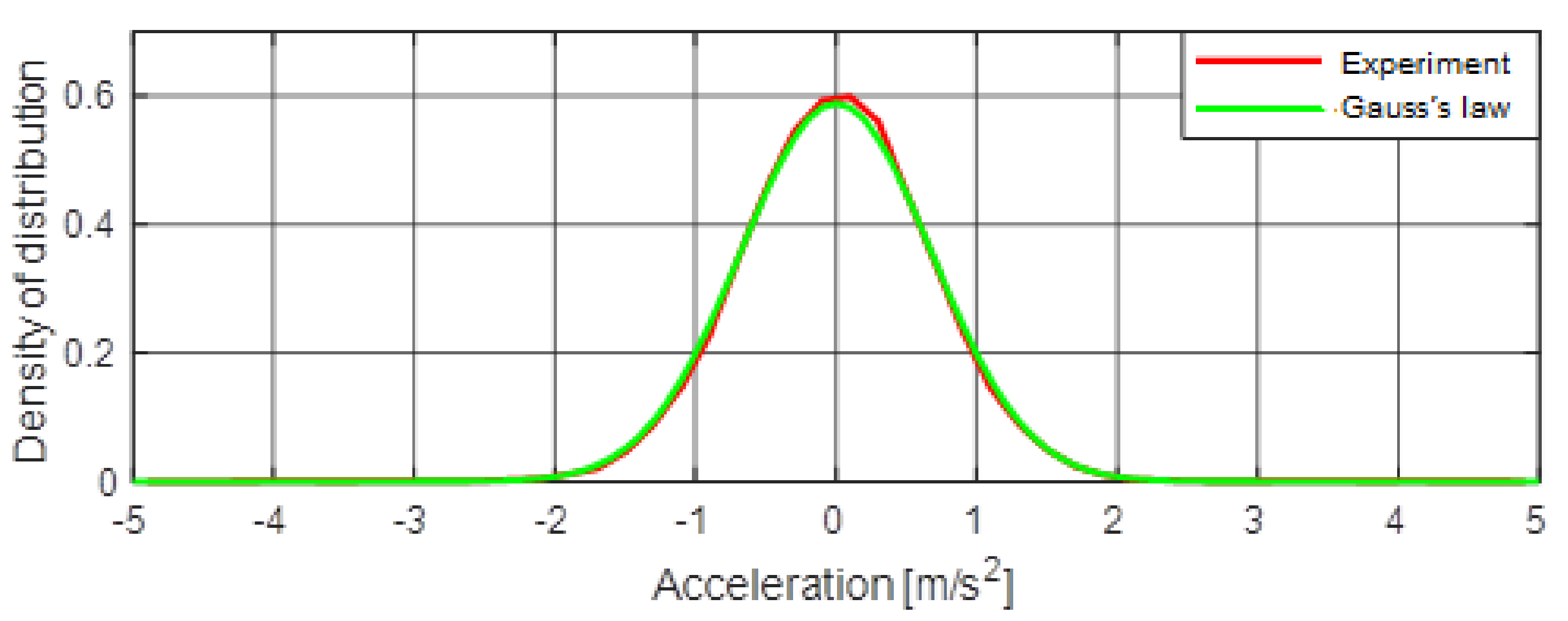
Figure 16.
Density of probability distribution, acceleration in vehicle CG.
Figure 16.
Density of probability distribution, acceleration in vehicle CG.
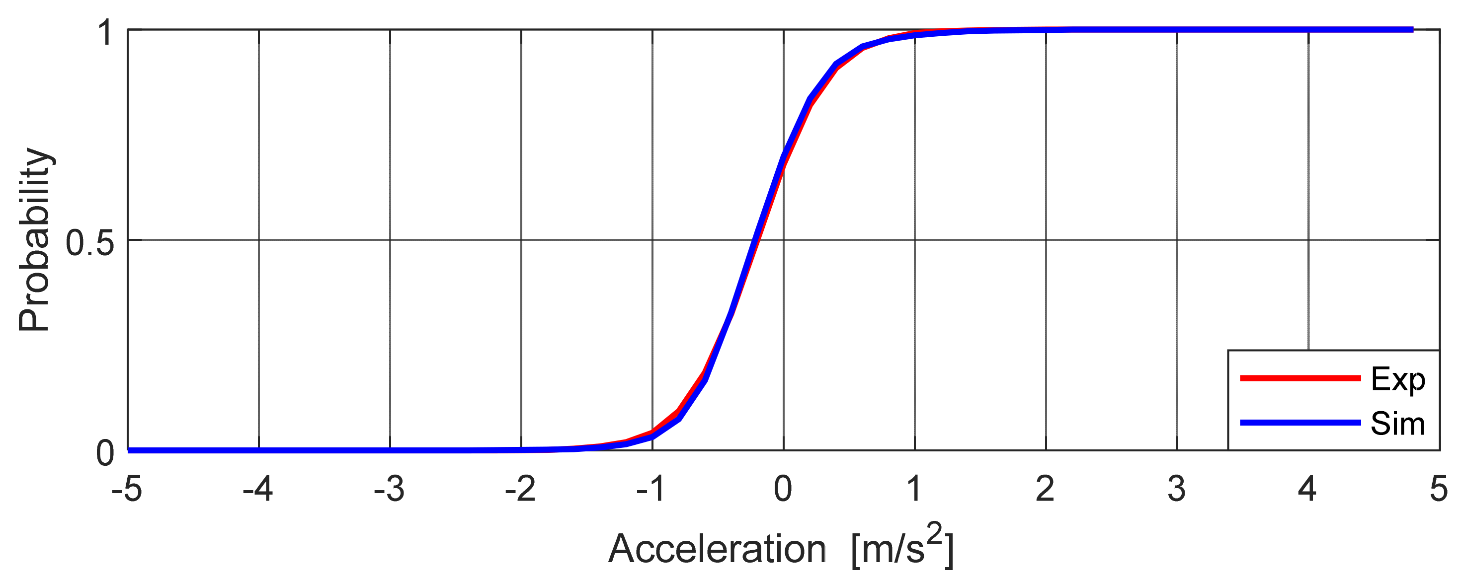
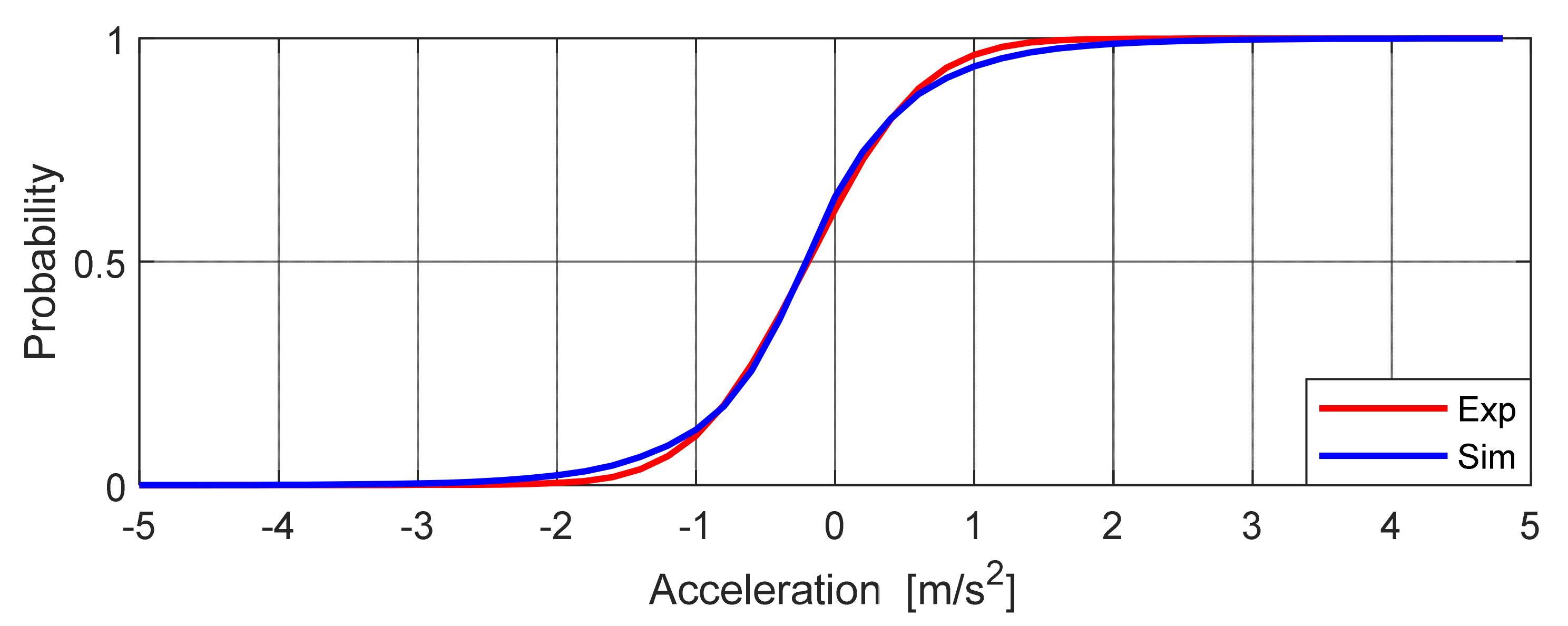
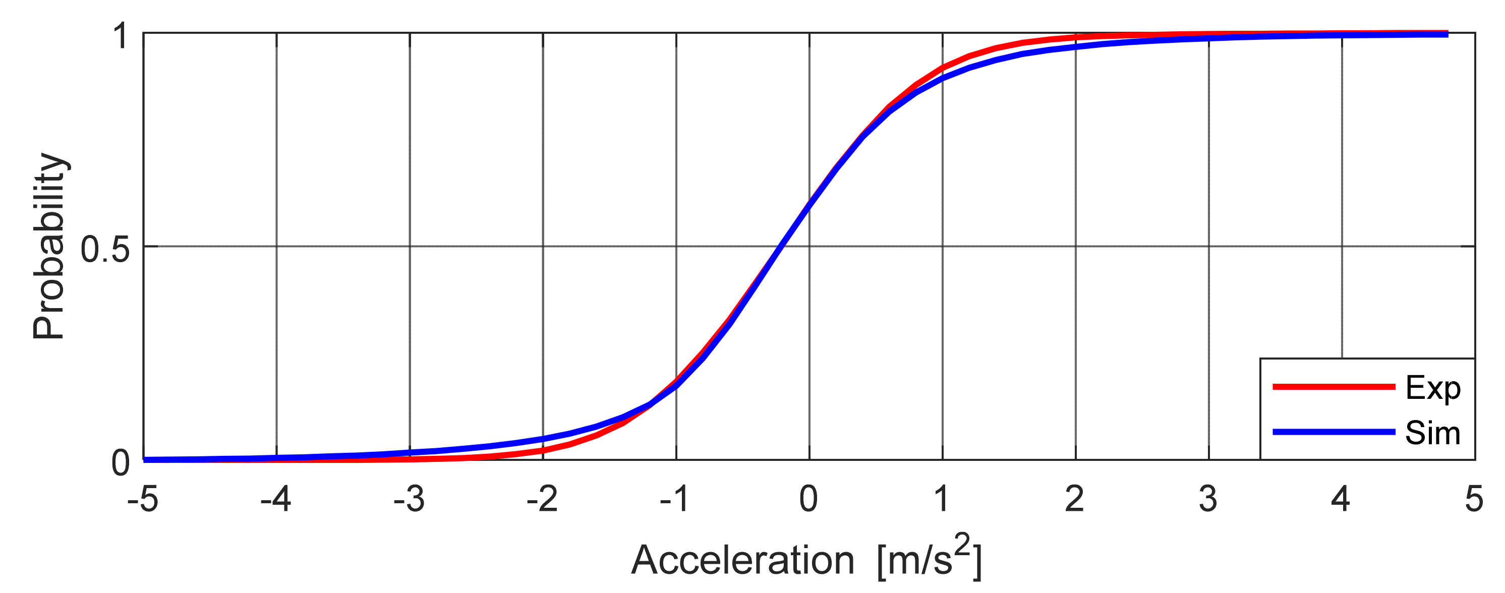
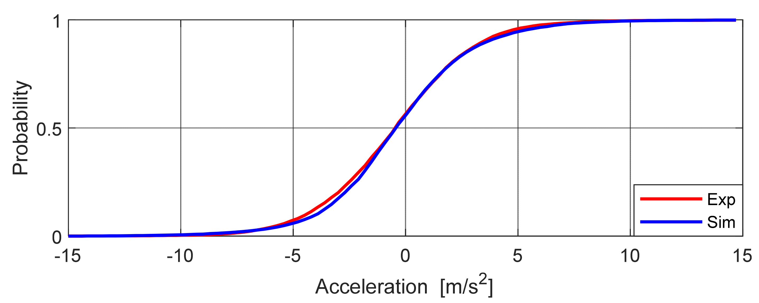
Figure 17.
Distribution function, acceleration in vehicle CG.
Figure 17.
Distribution function, acceleration in vehicle CG.
Figure 18.
PSD of vertical accelerations in vehicle CG.
Figure 18.
PSD of vertical accelerations in vehicle CG.
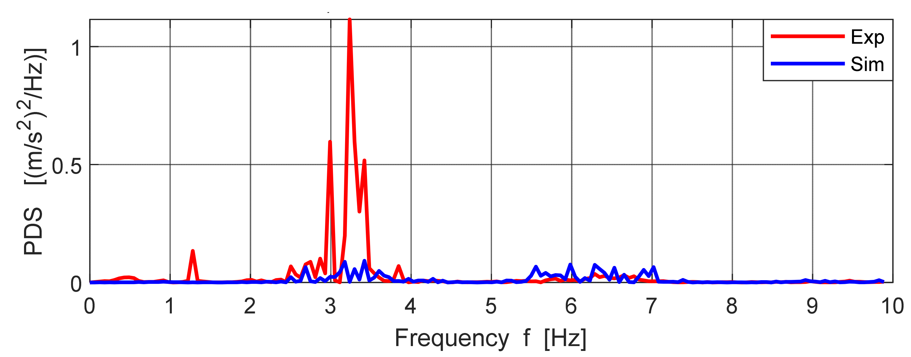
Figure 19.
PSD of vertical accelerations in vehicle CG, 0–10 Hz.
Figure 19.
PSD of vertical accelerations in vehicle CG, 0–10 Hz.
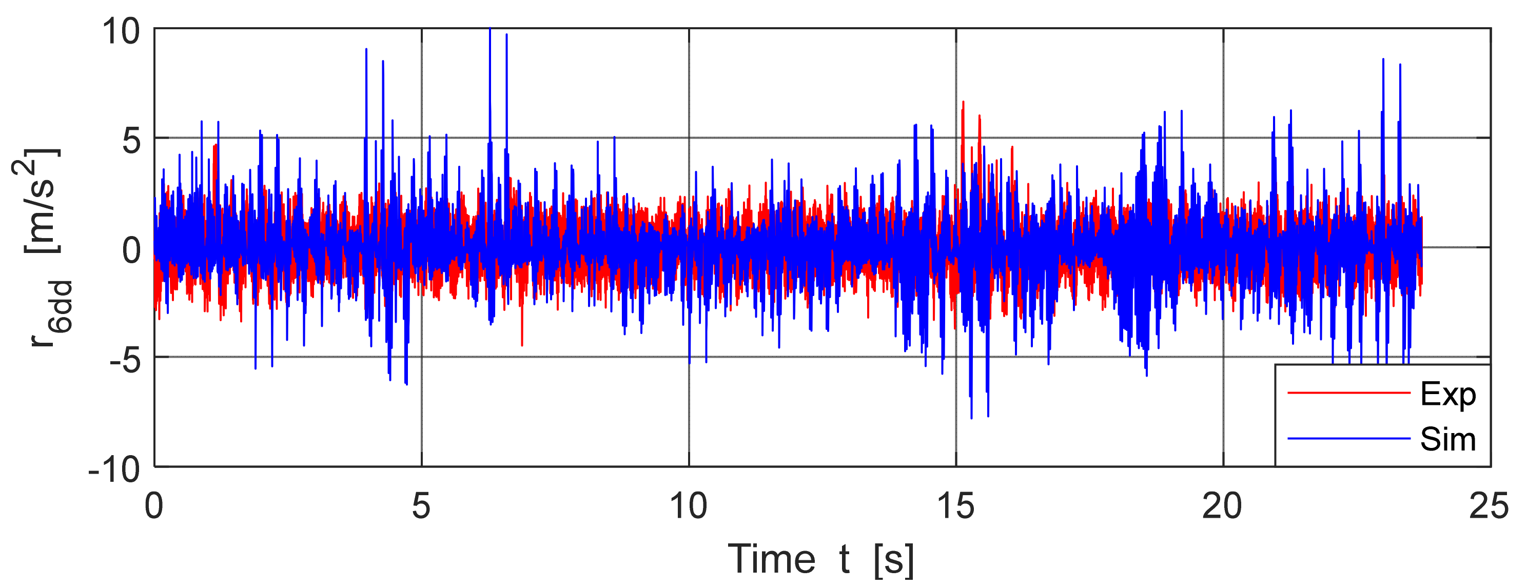
Figure 20.
Acceleration on right front axle, V = 15.18 km/h.
Figure 20.
Acceleration on right front axle, V = 15.18 km/h.
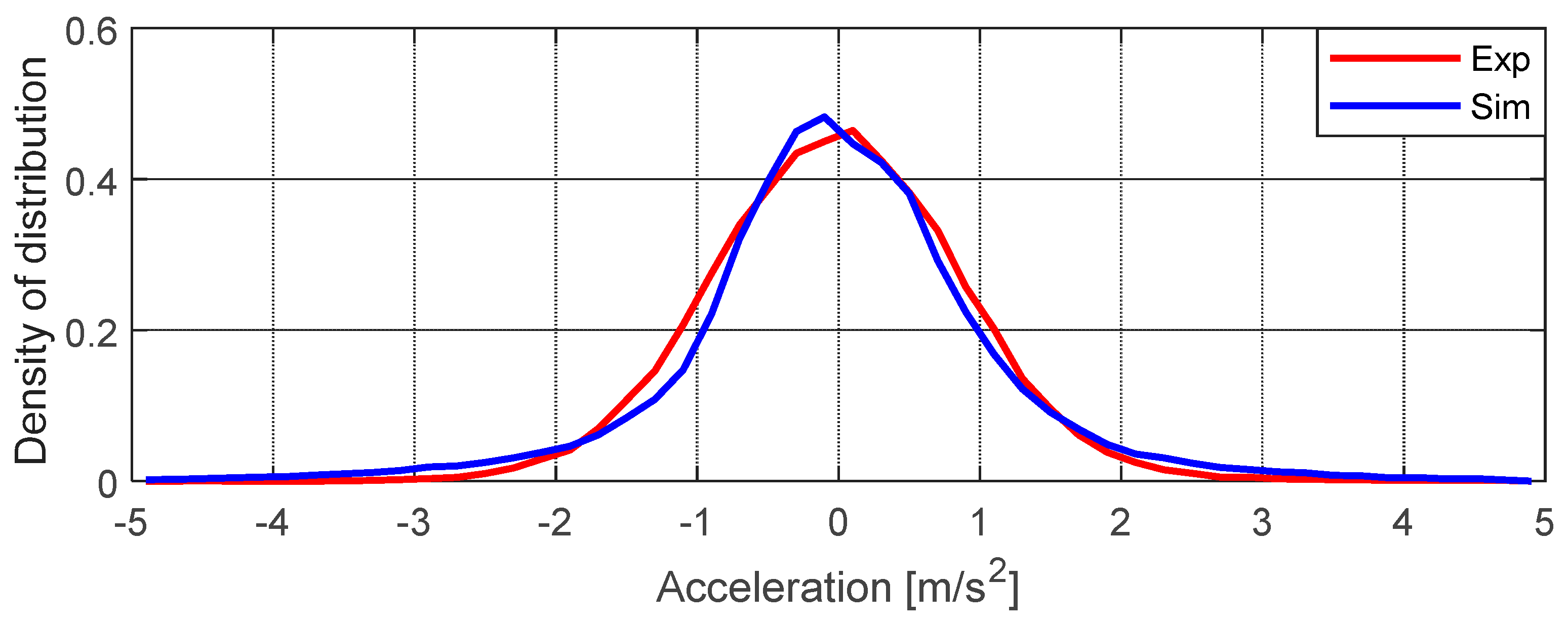
Figure 21.
Density of probability distribution, acceleration on vehicle front axle (FA).
Figure 21.
Density of probability distribution, acceleration on vehicle front axle (FA).
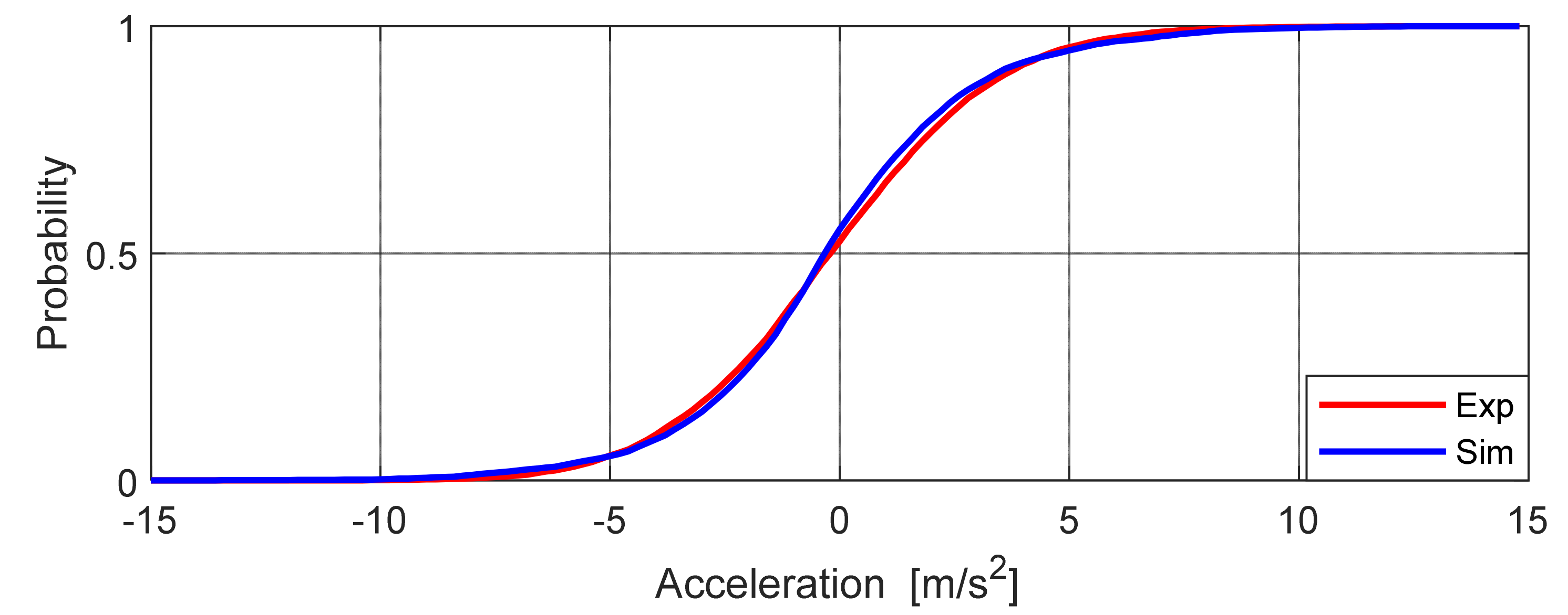
Figure 22.
Distribution function, acceleration on vehicle FA.
Figure 22.
Distribution function, acceleration on vehicle FA.
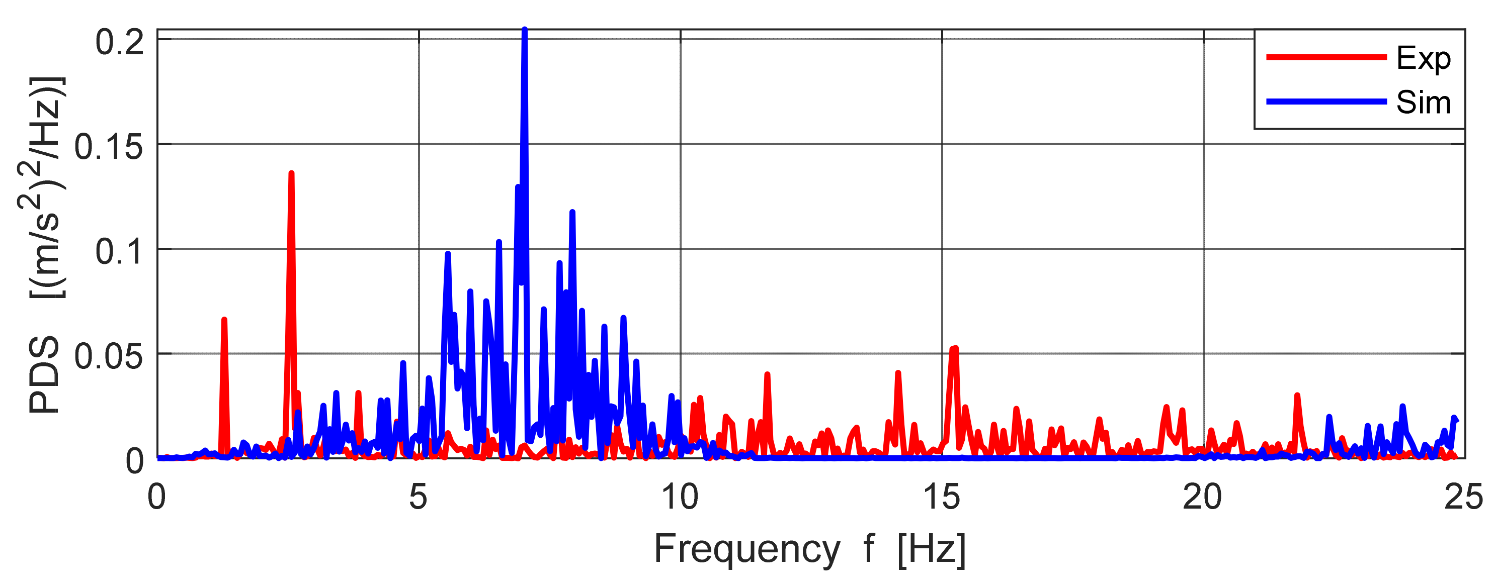
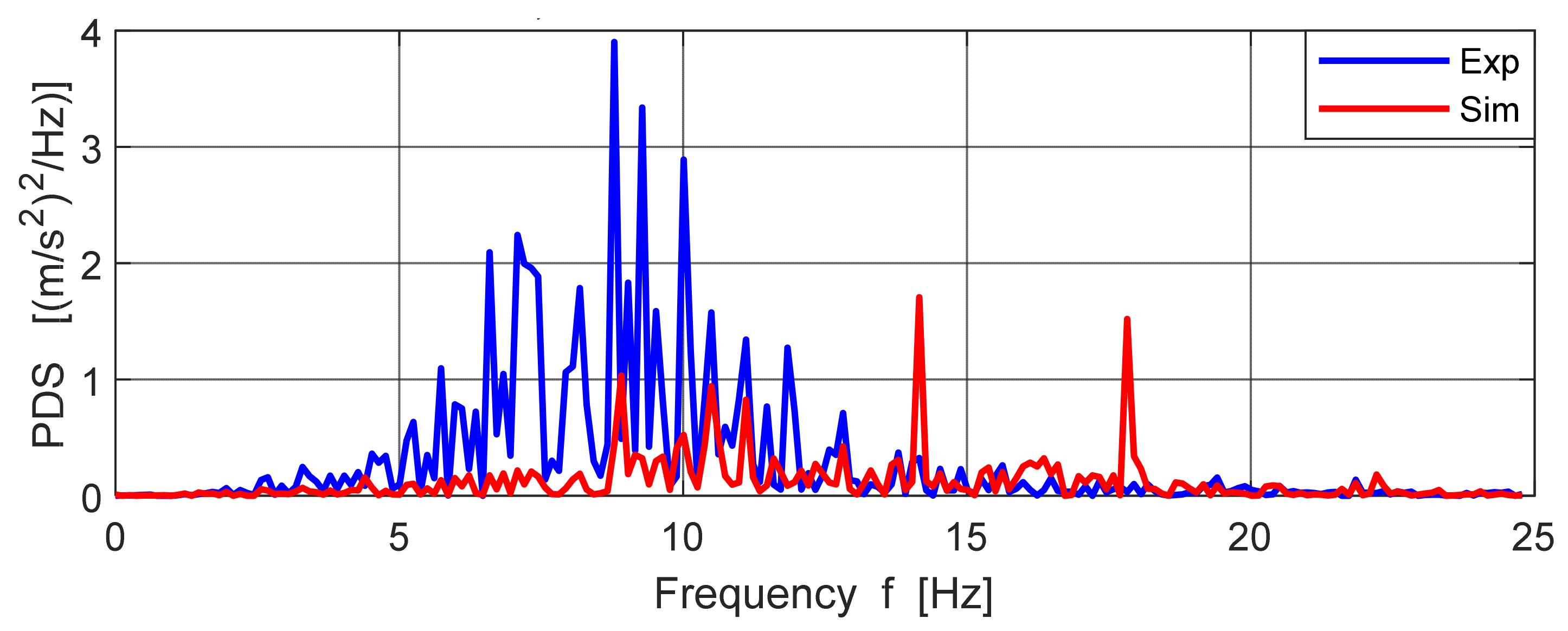
Figure 23.
PSD of vertical accelerations on vehicle FA, 0–25 Hz.
Figure 23.
PSD of vertical accelerations on vehicle FA, 0–25 Hz.
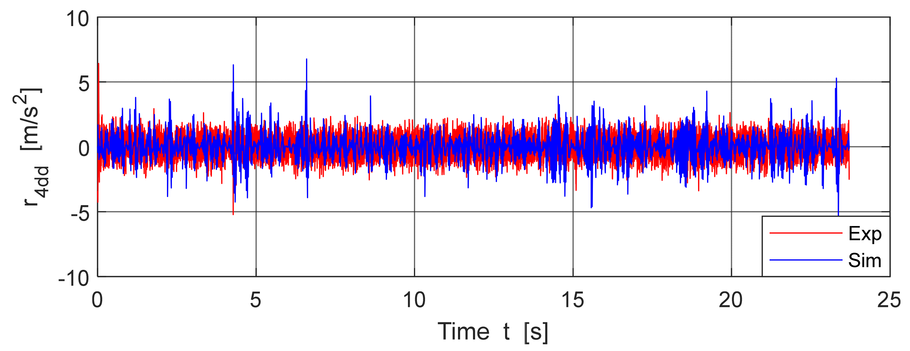
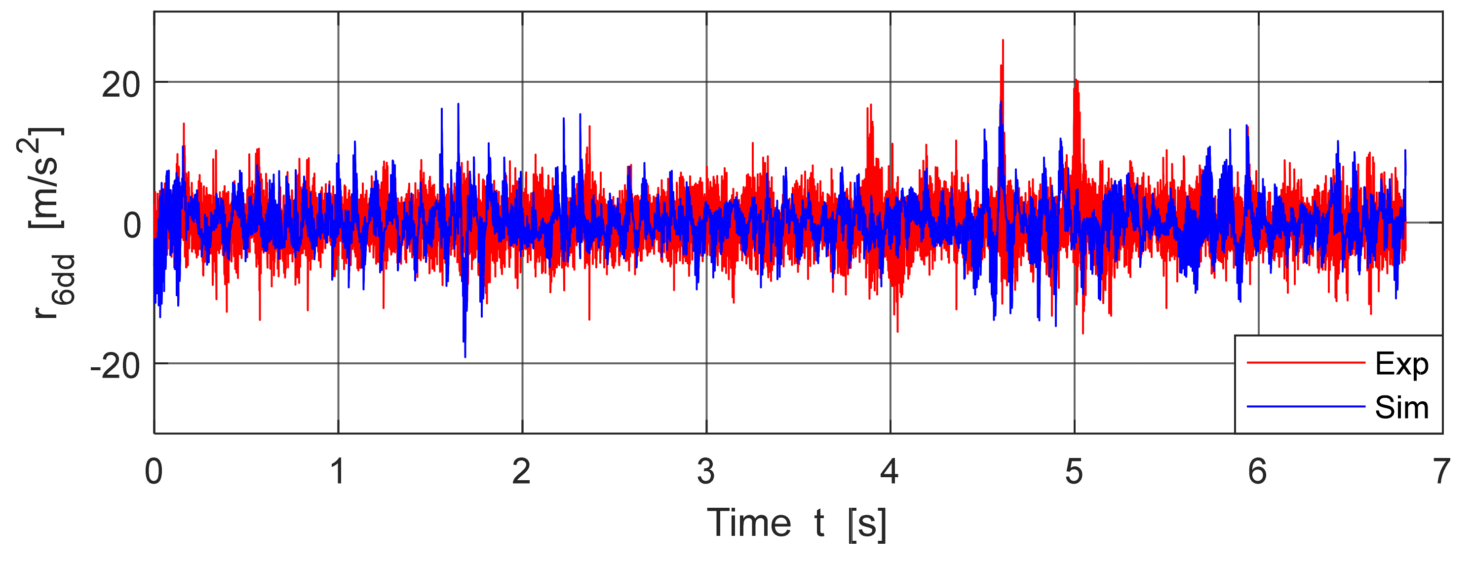
Figure 24.
Acceleration on right rear axle, V = 15.18 km/h.
Figure 24.
Acceleration on right rear axle, V = 15.18 km/h.
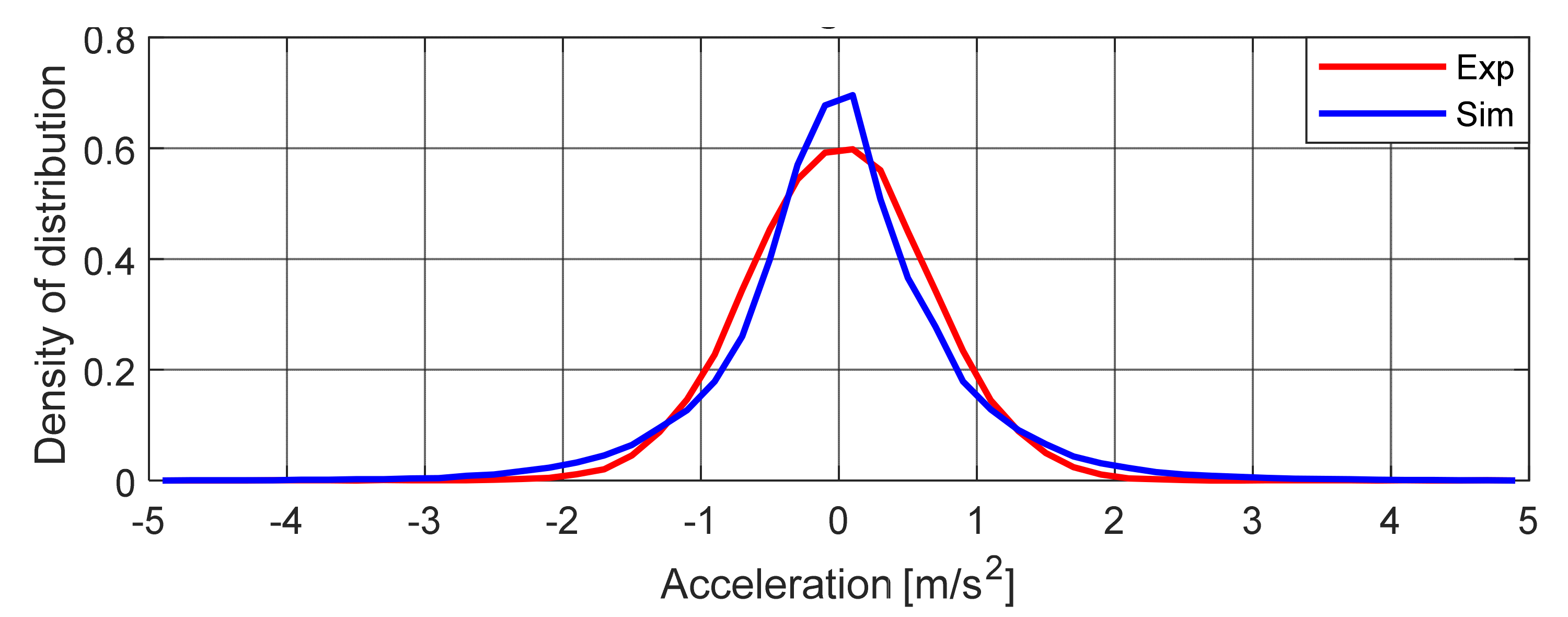
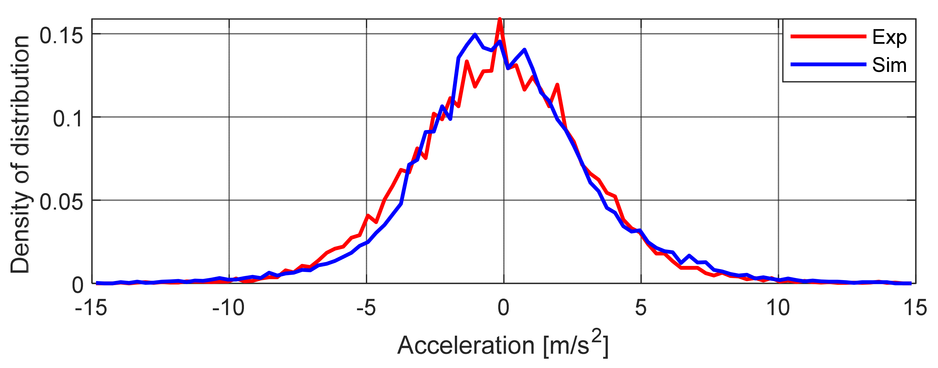
Figure 25.
Density of probability distribution, acceleration on vehicle rear axle (RA).
Figure 25.
Density of probability distribution, acceleration on vehicle rear axle (RA).
Figure 26.
Distribution function, acceleration on vehicle RA.
Figure 26.
Distribution function, acceleration on vehicle RA.
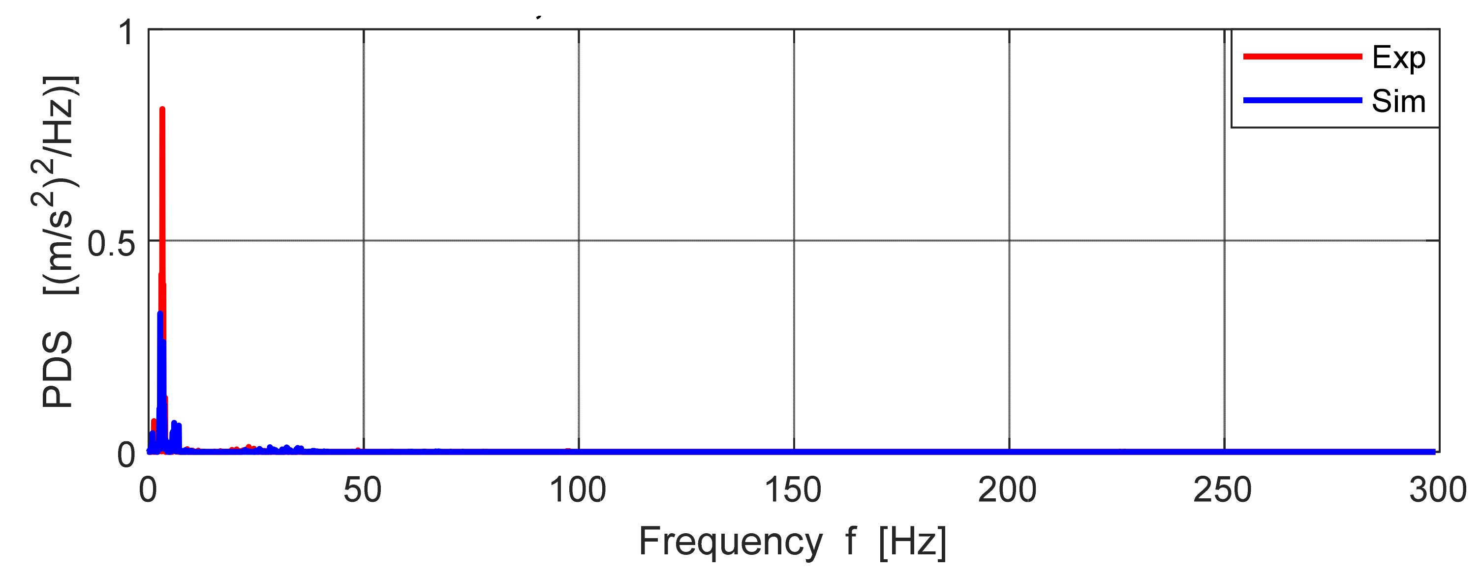
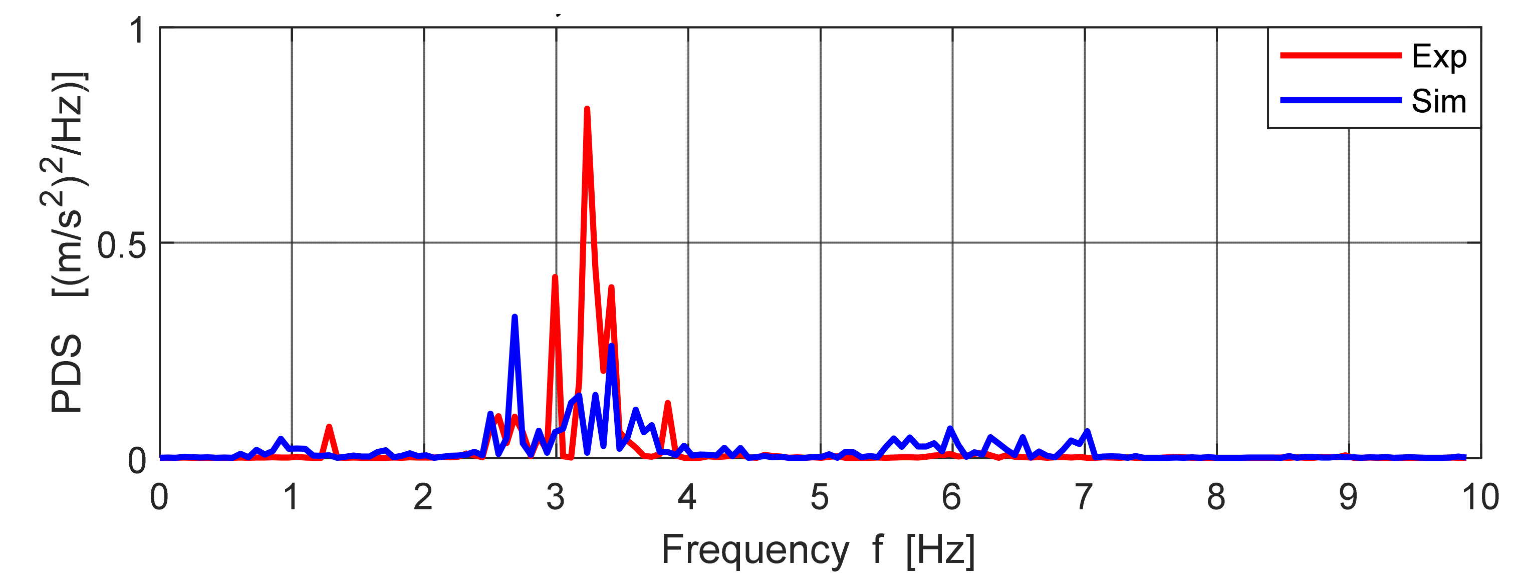
Figure 27.
PSD of vertical accelerations on vehicle RA, 0–10 Hz.
Figure 27.
PSD of vertical accelerations on vehicle RA, 0–10 Hz.
Figure 28.
Acceleration in the CG of vehicle sprung mass, V = 52.85 km/h.
Figure 28.
Acceleration in the CG of vehicle sprung mass, V = 52.85 km/h.
Figure 29.
Density of probability distribution, acceleration in vehicle CG.
Figure 29.
Density of probability distribution, acceleration in vehicle CG.
Figure 30.
Distribution function, acceleration in vehicle CG.
Figure 30.
Distribution function, acceleration in vehicle CG.
Figure 31.
PSD of vertical accelerations in vehicle CG, 0–10 Hz.
Figure 31.
PSD of vertical accelerations in vehicle CG, 0–10 Hz.
Figure 32.
Acceleration on right front axle, V = 52.95 km/h.
Figure 32.
Acceleration on right front axle, V = 52.95 km/h.
Figure 33.
Density of probability distribution, acceleration on vehicle FA.
Figure 33.
Density of probability distribution, acceleration on vehicle FA.
Figure 34.
Distribution function, acceleration on vehicle FA.
Figure 34.
Distribution function, acceleration on vehicle FA.
Figure 35.
PSD of vertical accelerations on vehicle FA, 0–25 Hz.
Figure 35.
PSD of vertical accelerations on vehicle FA, 0–25 Hz.
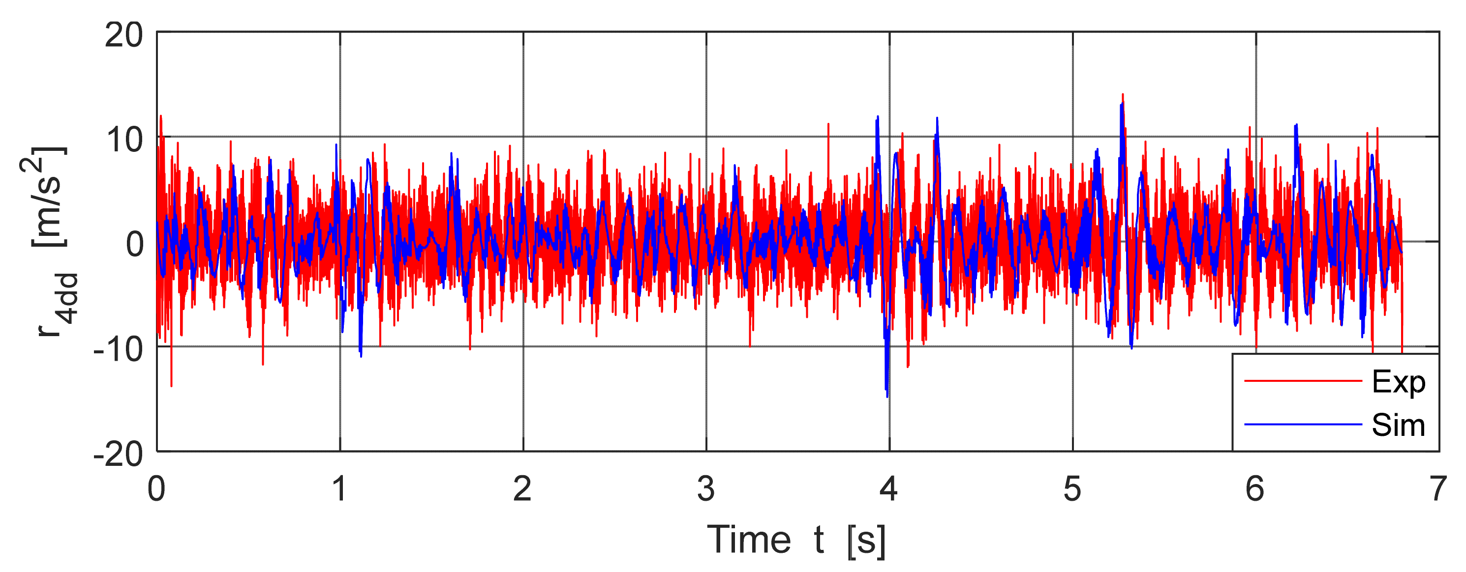
Figure 36.
Acceleration on right rear axle, V = 52.95 km/h.
Figure 36.
Acceleration on right rear axle, V = 52.95 km/h.
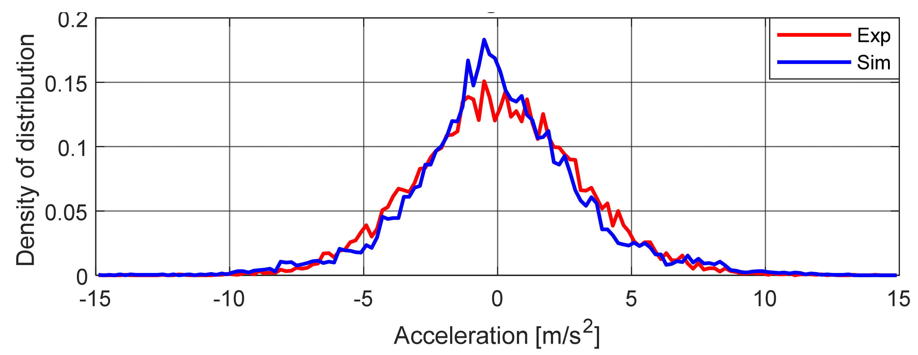
Figure 37.
Density of probability distribution, acceleration on vehicle RA.
Figure 37.
Density of probability distribution, acceleration on vehicle RA.
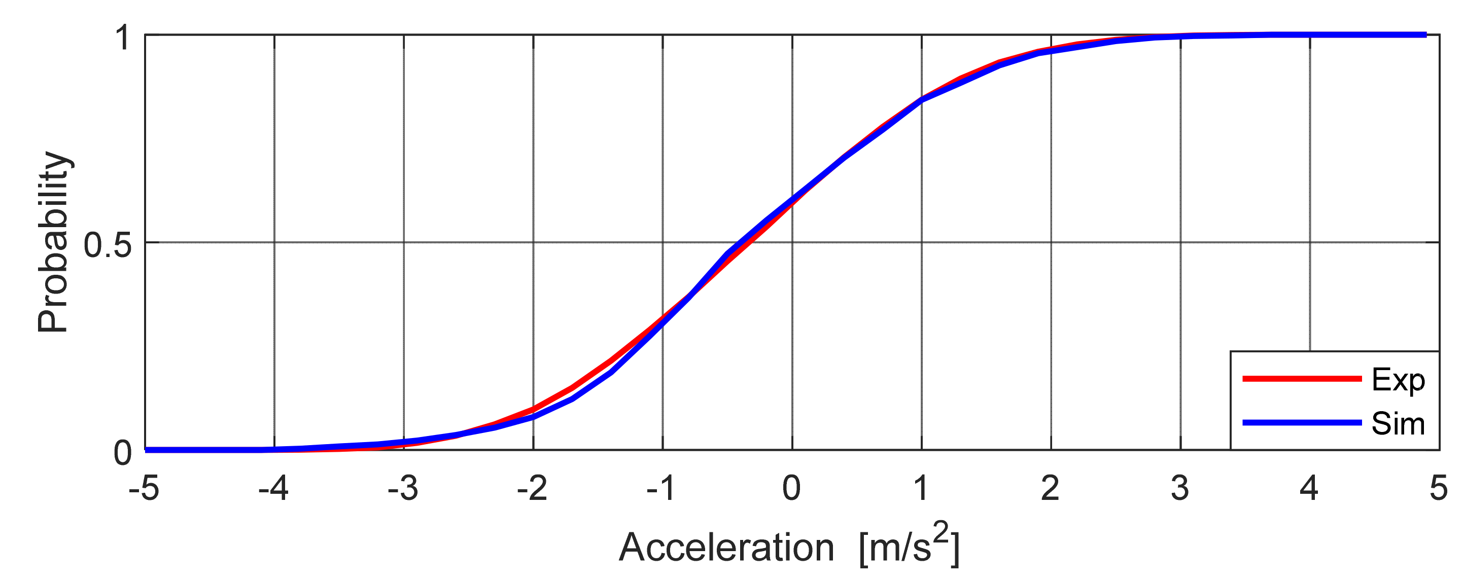
Figure 38.
Distribution function, acceleration on vehicle RA.
Figure 38.
Distribution function, acceleration on vehicle RA.
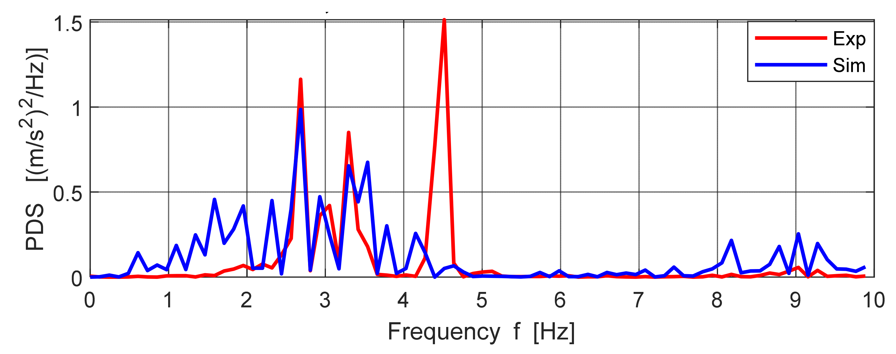
Figure 39.
PSD of vertical accelerations on vehicle RA, 0–10 Hz.
Figure 39.
PSD of vertical accelerations on vehicle RA, 0–10 Hz.
Figure 40.
Density of probability distribution, acceleration on vehicle FA, V = 15.18 km/h.
Figure 40.
Density of probability distribution, acceleration on vehicle FA, V = 15.18 km/h.
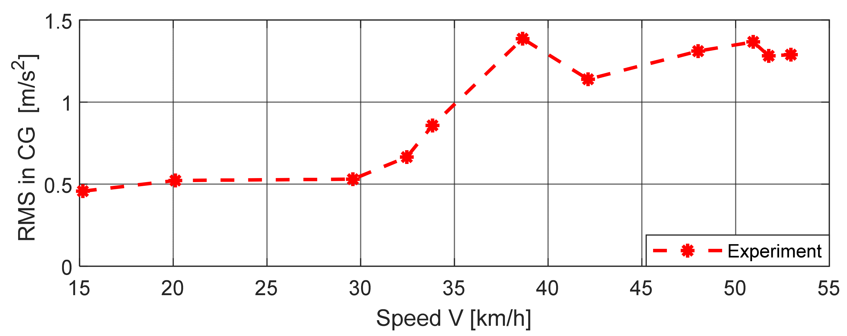
Figure 41.
RMS of acceleration in vehicle CG versus speed V.
Figure 41.
RMS of acceleration in vehicle CG versus speed V.
Table 1.
Statistical characteristics of the road profiles.
Table 1.
Statistical characteristics of the road profiles.
| | uL | uR |
|---|
| Mean value | 0.5874 mm | 0.3812 mm |
| Arithmetic mean deviation Ra | 8.1329 mm | 7.0686 mm |
| Root mean square (RMS) average deviation Rq | 10.0791 mm | 9.0668 mm |
| Dispersion σ2 | 101.5884 mm2 | 82.2073 mm2 |
| Effective value RMS | 10.0962 mm | 9.0748 mm |
| Asymmetry coefficient Rsk | 0.2454 | 0.1128 |
| Kurtosis Rku | 2.3314 | 2.6591 |
| The greatest depth of unevenness | −17.9348 mm | −18.8316 mm |
| The largest height of unevenness | 21.4085 mm | 20.9047 mm |
| Overall height of the profile | 39.3433 mm | 39.7364 mm |
Table 2.
Statistical characteristics of acceleration in vehicle CG.
Table 2.
Statistical characteristics of acceleration in vehicle CG.
| | Experiment | Simulation |
|---|
| Mean value
| −0.0019 mm | −0.0008 mm |
| Arithmetic mean deviation Ra | 0.3632 mm | 0.3469 mm |
| Root mean square average deviation Rq | 0.4688 mm | 0.4575 mm |
| Dispersion σ2 | 0.2198 mm2 | 0.2093 mm2 |
| Effective value RMS | 0.4688 mm | 0.4575 mm |
| Asymmetry coefficient Rsk | 0.4408 | 0.3230 |
| Kurtosis Rku | 3.7620 | 4.8537 |
| The greatest depth of record | −2.0433 mm | −2.1635 mm |
| The largest height of record | 2.4146 mm | 2.3314 mm |
| Overall height of the record | 4.4579 mm | 4.4950 mm |
Table 3.
Statistical characteristics of acceleration on right front axle.
Table 3.
Statistical characteristics of acceleration on right front axle.
| | Experiment | Simulation |
|---|
| Mean value
| 0.0031 mm | −0.0008 mm |
| Arithmetic mean deviation Ra | 0.5311 mm | 0.5878 mm |
| Root mean square average deviation Rq | 0.6786 mm | 0.8324 mm |
| Dispersion σ2 | 0.4605 mm2 | 0.6929 mm2 |
| Effective value RMS | 0.6786 mm | 0.8324 mm |
| Asymmetry coefficient Rsk | 0.0809 | 0.1851 |
| Kurtosis Rku | 4.7239 | 6.8217 |
| The greatest depth of record | −5.2235 mm | −5.6434 mm |
| The largest height of record | 6.4155 mm | 6.7649 mm |
| Overall height of the record | 11.6390 mm | 12.4084 mm |
Table 4.
Statistical characteristics of acceleration on right rear axle.
Table 4.
Statistical characteristics of acceleration on right rear axle.
| | Experiment | Simulation |
|---|
| Mean value
| −0.0062 mm | −0.0003 mm |
| Arithmetic mean deviation Ra | 0.7076 mm | 0.8128 mm |
| Root mean square average deviation Rq | 0.9106 mm | 1.1605 mm |
| Dispersion σ2 | 0.8292 mm2 | 1.3468 mm2 |
| Effective value RMS | 0.9106 mm | 1.1605 mm |
| Asymmetry coefficient Rsk | 0.2835 | 0.1368 |
| Kurtosis Rku | 4.5032 | 7.6179 |
| The greatest depth of record | −4.6194 mm | −7.8089 mm |
| The largest height of record | 6.6533 mm | 10.1296 mm |
| Overall height of the record | 11.2728 mm | 17.9385 mm |
Table 5.
Statistical characteristics of acceleration in vehicle CG.
Table 5.
Statistical characteristics of acceleration in vehicle CG.
| | Experiment | Simulation |
|---|
| Mean value
| −0.0296 mm | −0.0060 mm |
| Arithmetic mean deviation Ra | 1.0412 mm | 1.0346 mm |
| Root mean square average deviation Rq | 1.2769 mm | 1.2843 mm |
| Dispersion σ2 | 1.6307 mm2 | 1.6495 mm2 |
| Effective value RMS | 1.2773 mm | 1.2843 mm |
| Asymmetry coefficient Rsk | 0.0532 | 0.0676 |
| Kurtosis Rku | 2.6251 | 2.9134 |
| The greatest depth of record | −3.8163 mm | −3.8200 mm |
| The largest height of record | 4.5049 mm | 3.8873 mm |
| Overall height of the record | 8.3213 mm | 7.7074 mm |
Table 6.
Statistical characteristics of acceleration on vehicle FA.
Table 6.
Statistical characteristics of acceleration on vehicle FA.
| | Experiment | Simulation |
|---|
| Mean value
| 0.0396 mm | −0.0076 mm |
| Arithmetic mean deviation Ra | 2.4080 mm | 2.3237 mm |
| Root mean square average deviation Rq | 3.0531 mm | 3.1212 mm |
| Dispersion σ2 | 9.3214 mm2 | 9.7419 mm2 |
| Effective value RMS | 3.0533 mm | 3.1212 mm |
| Asymmetry coefficient Rsk | 0.0934 | 0.1137 |
| Kurtosis Rku | 3.3311 | 4.3811 |
| The greatest depth of record | −13.8083 mm | −14.8321 mm |
| The largest height of record | 14.0480 mm | 13.1869 mm |
| Overall height of the record | 27.8563 mm | 28.0191 mm |
Table 7.
Statistical characteristics of acceleration on vehicle RA.
Table 7.
Statistical characteristics of acceleration on vehicle RA.
| | Experiment | Simulation |
|---|
| Mean value
| −0.1588 mm | −0.0184 mm |
| Arithmetic mean deviation Ra | 2.4934 mm | 2.4533 mm |
| Root mean square average deviation Rq | 3.2557 mm | 3.2746 mm |
| Dispersion σ2 | 10.5998 mm2 | 10.7233 mm2 |
| Effective value RMS | 3.2596 mm | 3.2746 mm |
| Asymmetry coefficient Rsk | 0.2650 | 0.1038 |
| Kurtosis Rku | 5.1084 | 4.8027 |
| The greatest depth of record | −15.7769 mm | −19.1264 mm |
| The largest height of record | 25.9766 mm | 17.1971 mm |
| Overall height of the record | 41.7536 mm | 36.3236 mm |
Table 8.
Differences (Simulation–Experiment) of effective value RMS in (%).
Table 8.
Differences (Simulation–Experiment) of effective value RMS in (%).
| | Difference (Simulation–Experiment) in (%) of Experiment |
|---|
| Sensor | A1-CG | A2-FA | A3-RA |
| V = 15.18 km/h | −2.41% | +22.66% | +27.44% |
| V = 52.95 km/h | +0.55% | +2.22% | +0.46% |


