
Solving Regression Problems with Intelligent Machine Learner for Engineering Informatics


Abstract
:1. Introduction
2. Literature Review
3. Applied Machine Learning
3.1. Classification and Regression Model
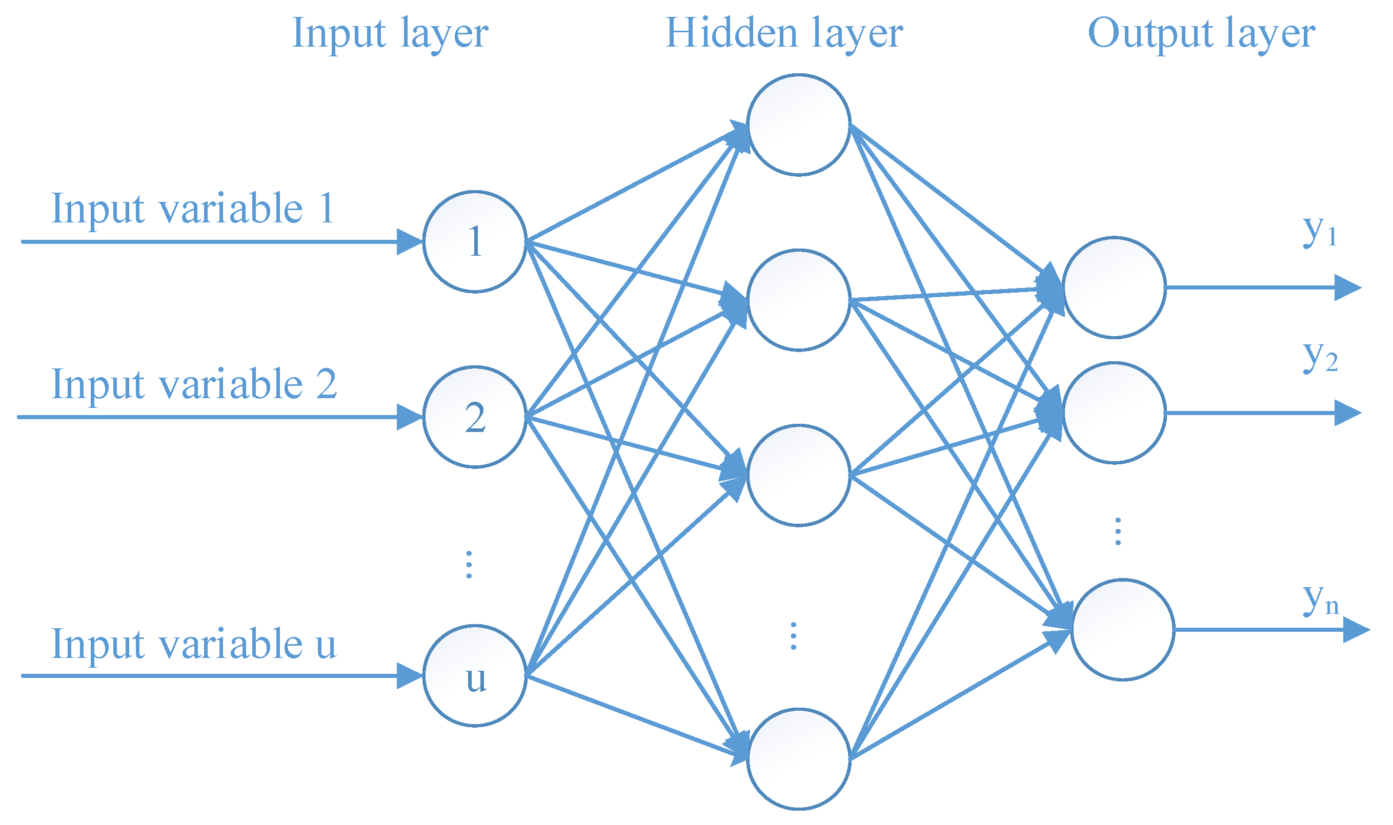
3.1.1. Artificial Neural Network (ANN)
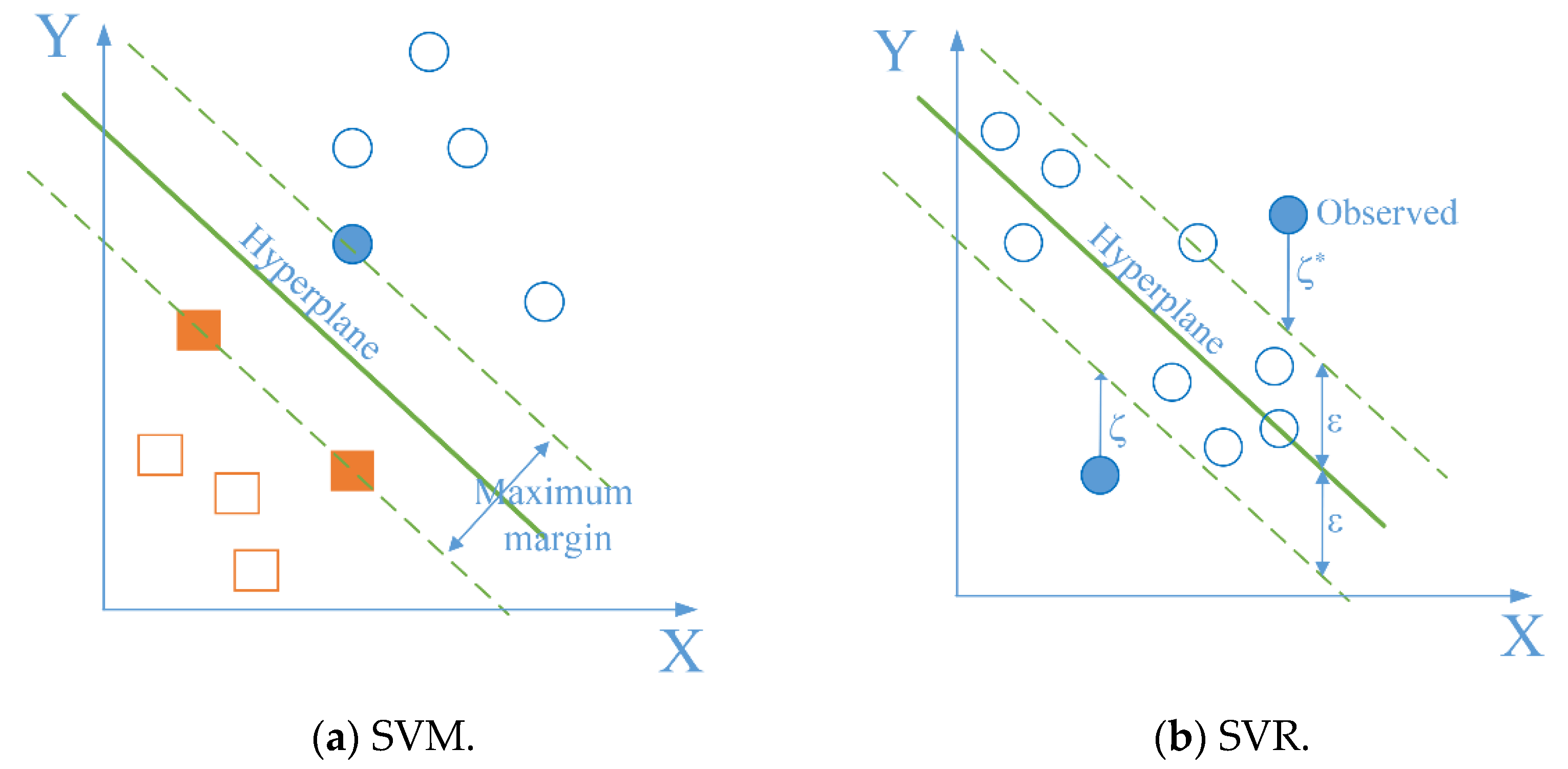
3.1.2. Support Vector Machine (SVM) and Support Vector Regression (SVR)
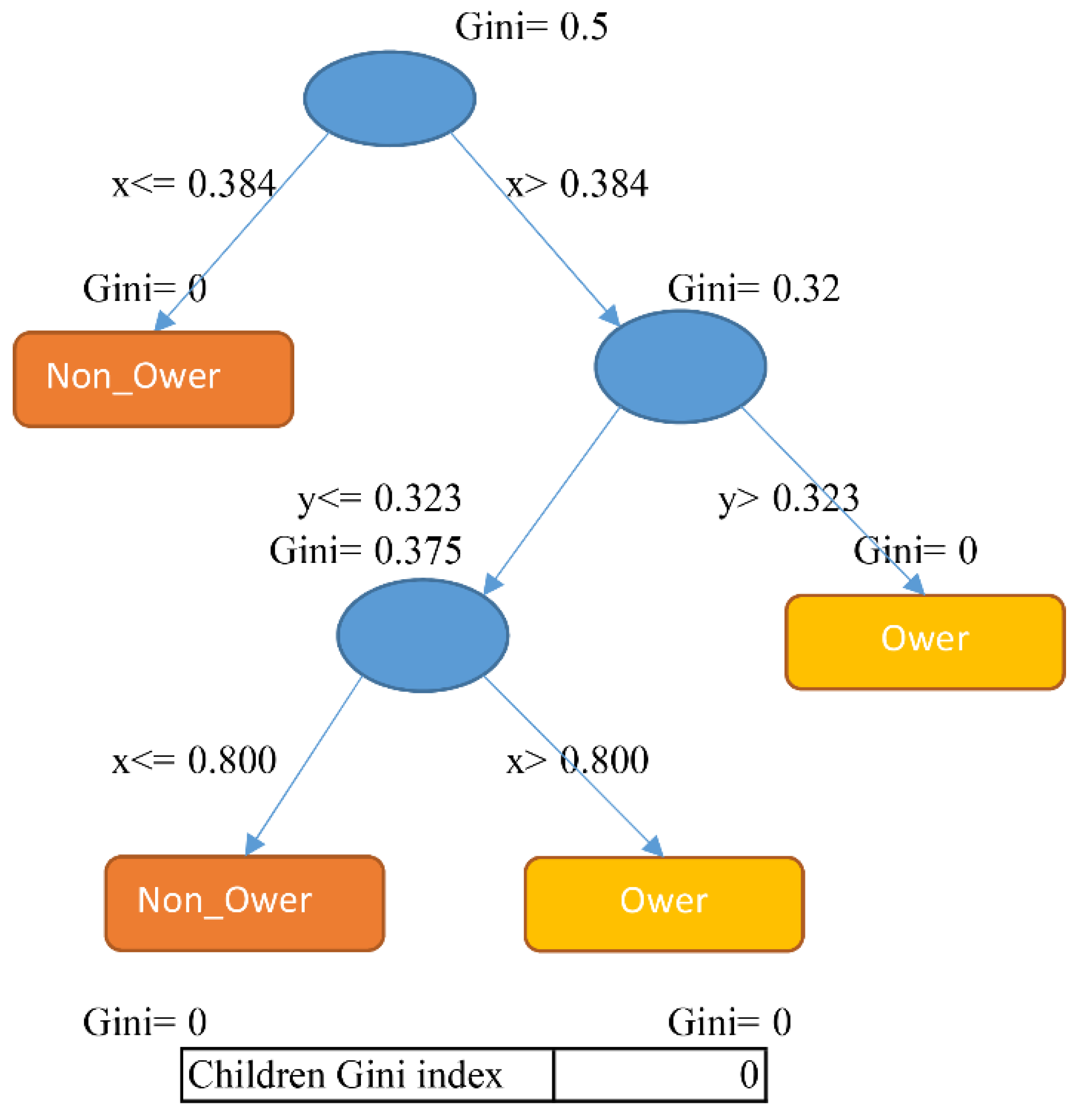
3.1.3. Classification and Regression Tree (CART)
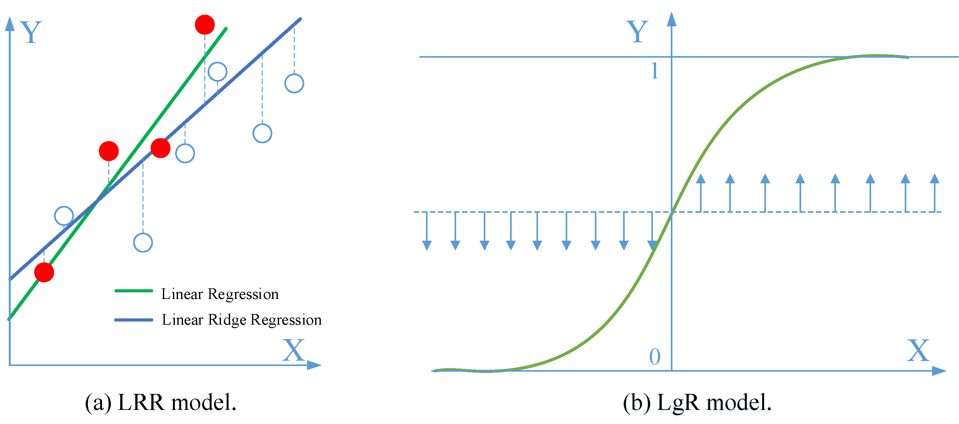
3.1.4. Linear Ridge Regression (LRR) and Logistic Regression (LgR)
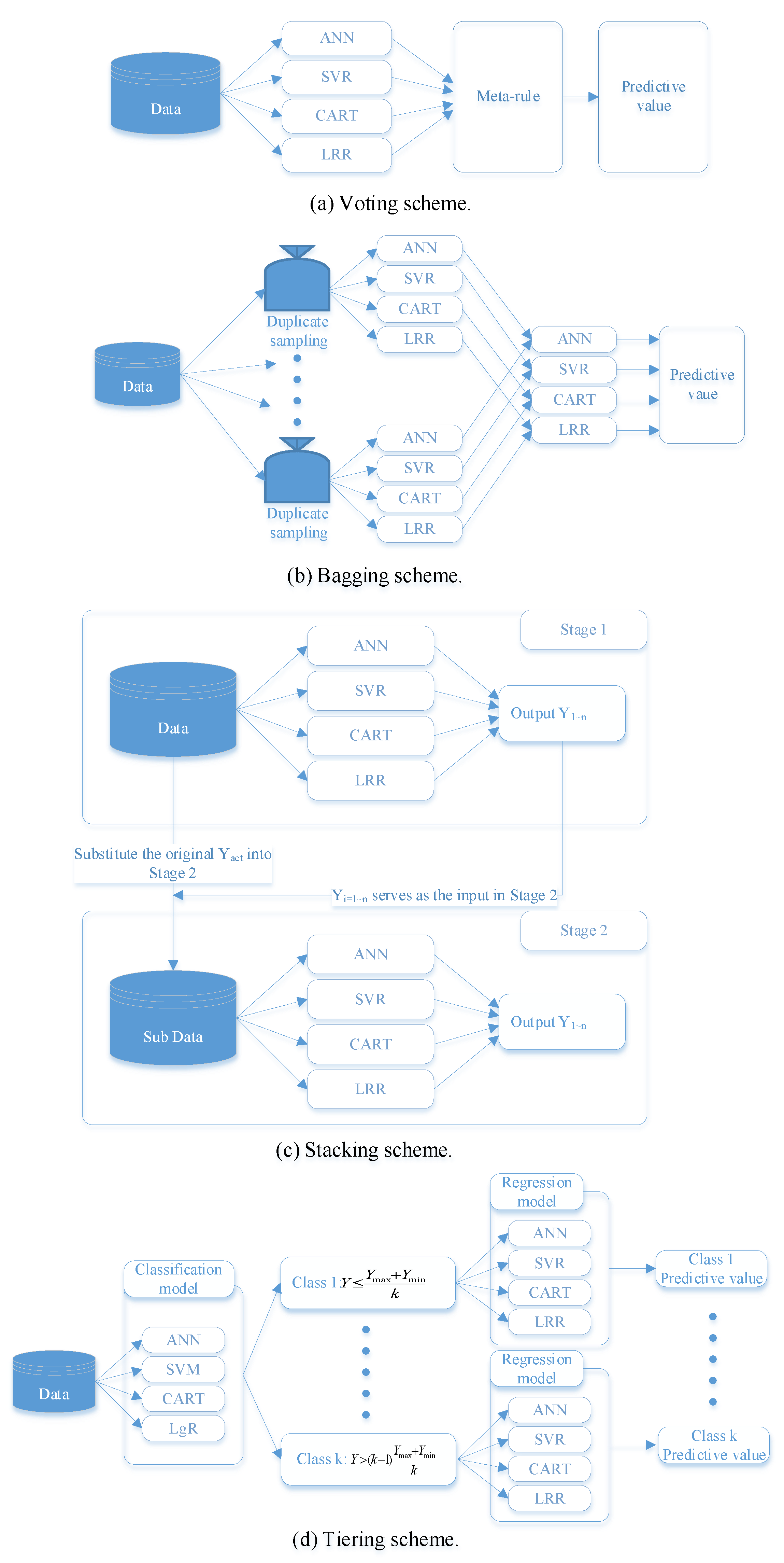
3.2. Ensemble Regression Model
- Voting: The voting ensemble model combines the outputs of the single models using a meta-rule. The mean of the output values is used in this study. According to the adopted ML models, 11 voting models are trained in this study, including (1) ANN + SVR, (2) ANN + CART, (3) ANN + LRR, (4) SVR + CART, (5) SVR + LRR, (6) CART + LRR, (7) ANN + SVR + CART, (8) ANN + CART + LRR, (9) ANN + CART + LRR, (10) SVR + CART + LRR, (11) ANN + SVR + CART + LRR. Figure 5a presents the voting ensemble model.
- Bagging: The bagging ensemble model duplicates samples at random, and each regression model predicts values from the samples independently. The meta-rule is applied to all of the outputs in this study. Bagging ensemble model is depicted at Figure 5b.
- Stacking: The stacking ensemble model is a two-stage model, and Figure 5c describes the principle of the model. In stage 1, each single model predicts one output value. Then, these outputs are used as inputs to train a model by these machine learning techniques again to make a meta-prediction in stage 2. There are four stacking models herein, including ANN (ANN, SVR, CART, LRR); SVR (ANN, SVR, CART, LRR); CART (ANN, SVR, CART, LRR); LRR (ANN, SVR, CART, LRR).
- Tiering: Figure 5d illustrates the tiering ensemble model. There are two tiers inside a tiering ensemble model in this study. The first tier is to classify data into classes on the basis of value [18]. Machine learning technique in the first tier for classifying data needs to be identified. After classifying the data, the regression machine learning is used to train each data (Sub Data) of each class (second tier) to predict results. In the iML, we developed three types of models, including 2-class, 3-class, and 4-class. The equation for calculating value is:where T is standard value, is the number of classes, and and are the maximum and minimum of actual values, respectively.
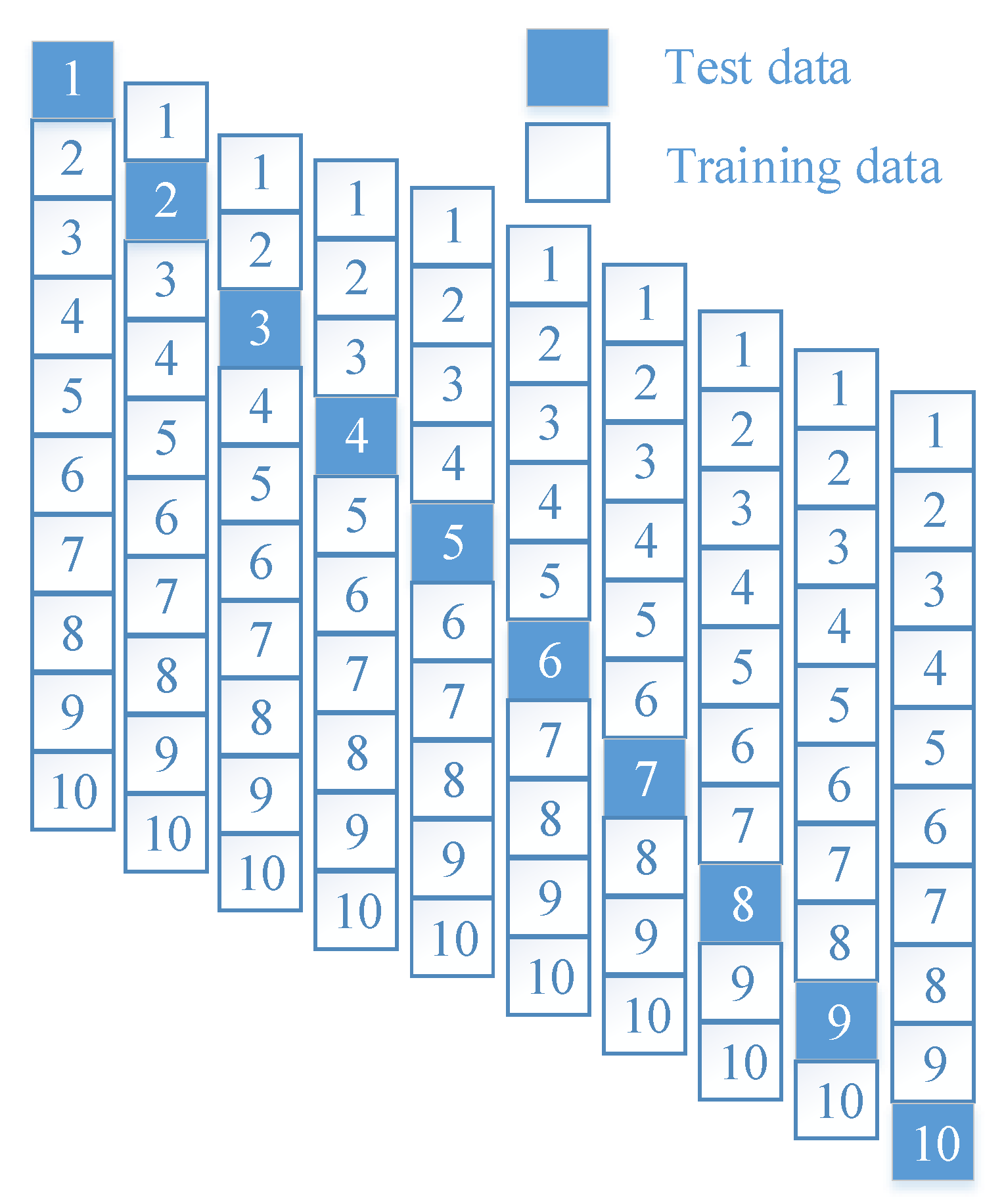
3.3. K-Fold Cross Validation
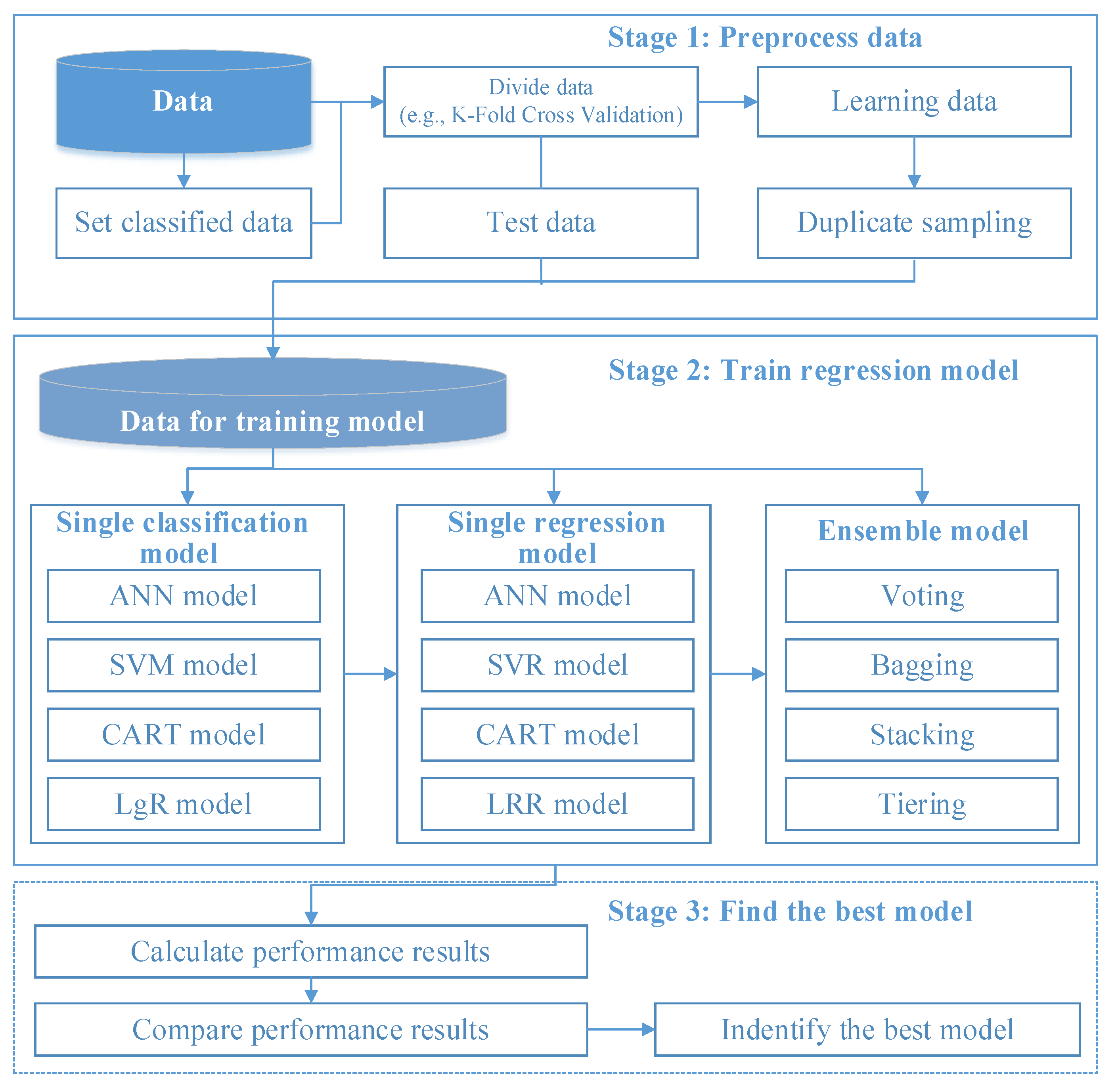
3.4. Intelligent Machine Learner Framework
4. Mathematical Formulas for Performance Measures
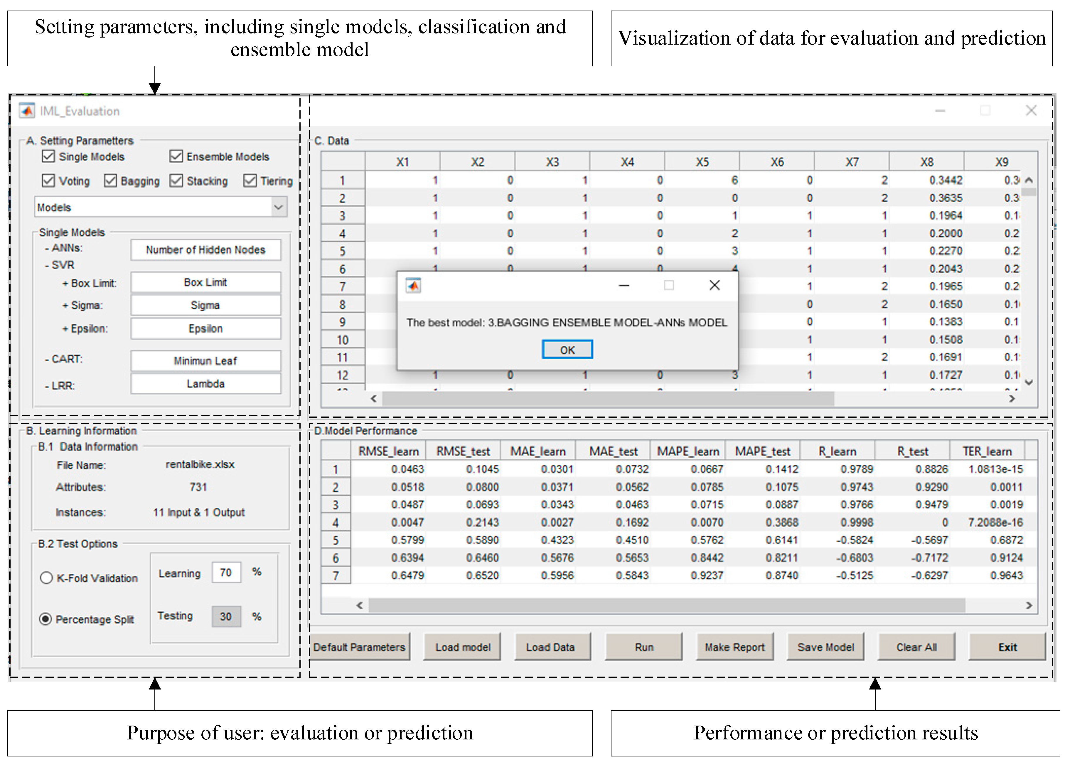
5. Design and Implementation of iML Interface
6. Benchmarks between iML and WEKA
6.1. Publicly Available Datasets
6.2. Hold-Out Validation
6.3. K-Fold Cross-Validation
6.4. Discussion
7. Numerical Experiments
7.1. Enterprise Resource Planning Software Development Effort
7.1.1. Variable Selection
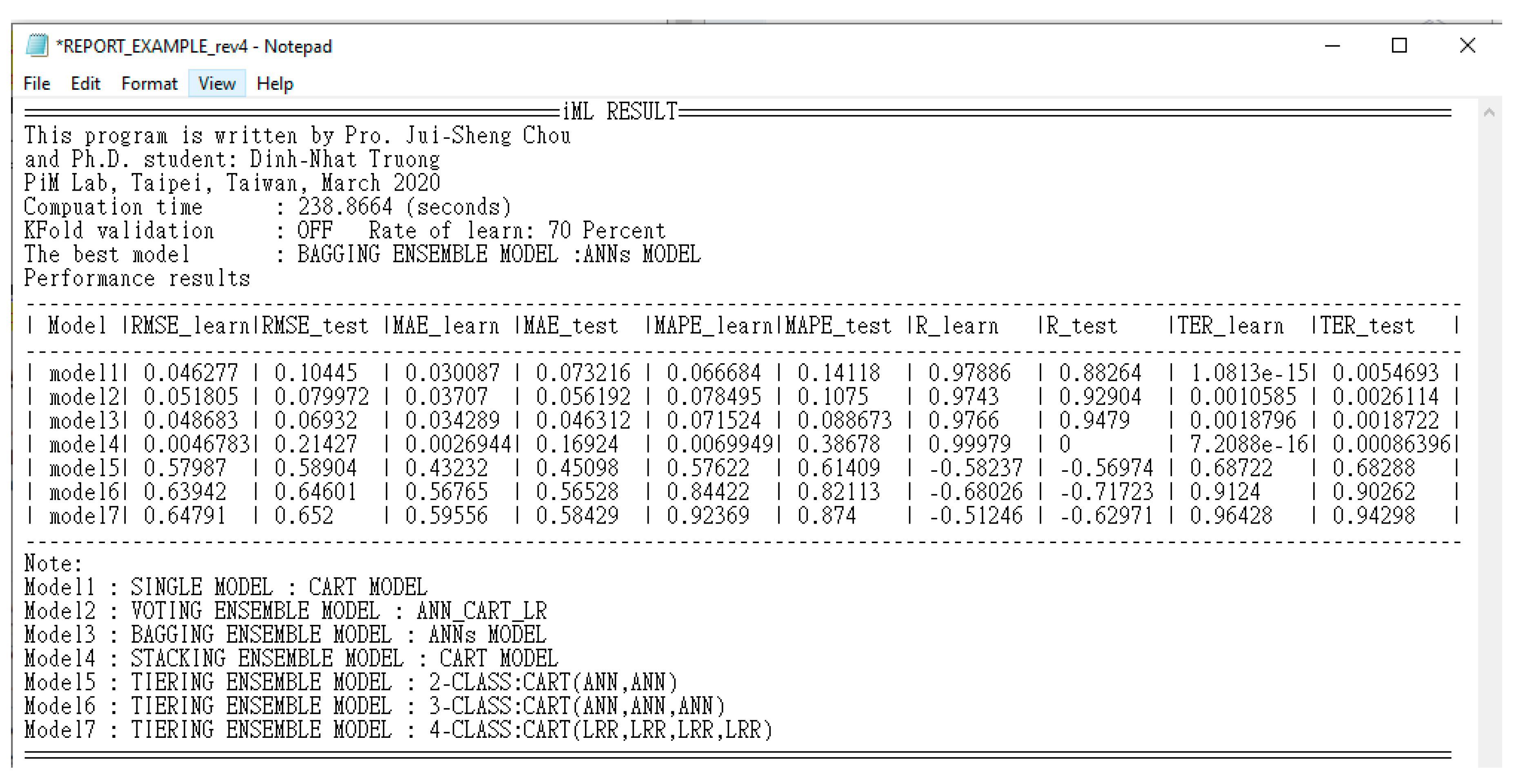
7.1.2. iML Results
7.2. Experiments on Industrial Datasets
7.2.1. Performance of CPU Processors
7.2.2. Daily Demand Forecasting Orders
7.2.3. Total Hourly-Shared Bike Rental per Days
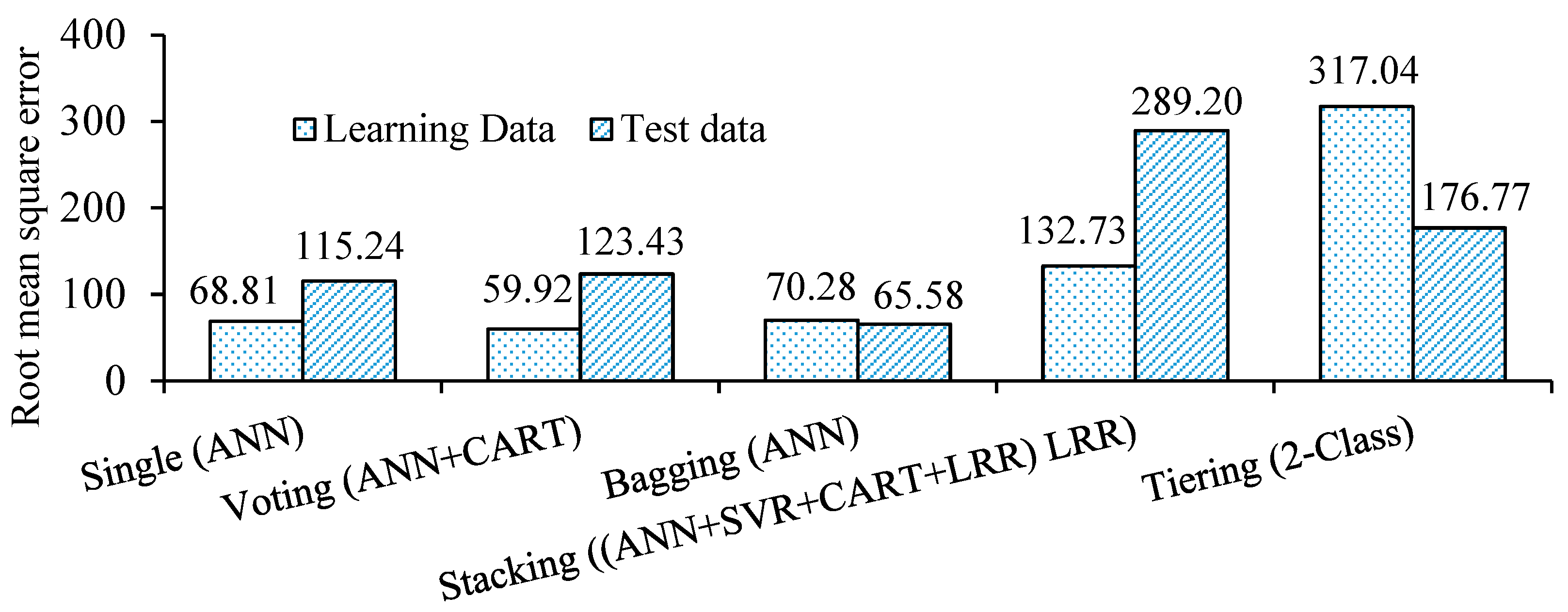
7.2.4. Performance Results
8. Conclusions and Future Work
Author Contributions
Funding
Data Availability Statement
Acknowledgments
Conflicts of Interest
References
- Chou, J.-S.; Cheng, M.-Y.; Wu, Y.-W.; Wu, C.-C. Forecasting enterprise resource planning software effort using evolutionary support vector machine inference model. Int. J. Proj. Manag. 2012, 30, 967–977. [Google Scholar] [CrossRef]
- Pham, A.-D.; Ngo, N.-T.; Nguyen, Q.-T.; Truong, N.-S. Hybrid machine learning for predicting strength of sustainable concrete. Soft Comput. 2020. [Google Scholar] [CrossRef]
- Cheng, M.-Y.; Chou, J.-S.; Cao, M.-T. Nature-inspired metaheuristic multivariate adaptive regression splines for predicting refrigeration system performance. Soft Comput. 2015, 21, 477–489. [Google Scholar] [CrossRef]
- Li, Y.; Lei, G.; Bramerdorfer, G.; Peng, S.; Sun, X.; Zhu, J. Machine Learning for Design Optimization of Electromagnetic Devices: Recent Developments and Future Directions. Appl. Sci. 2021, 11, 1627. [Google Scholar] [CrossRef]
- Piersanti, S.; Orlandi, A.; Paulis, F.d. Electromagnetic Absorbing Materials Design by Optimization Using a Machine Learning Approach. IEEE Trans. Electromagn. Compat. 2018, 1–8. [Google Scholar] [CrossRef]
- Chou, J.S.; Pham, A.D. Smart artificial firefly colony algorithm-based support vector regression for enhanced forecasting in civil engineering. Comput.-Aided Civ. Infrastruct. Eng. 2015, 30, 715–732. [Google Scholar] [CrossRef]
- Cheng, M.-Y.; Prayogo, D.; Wu, Y.-W. A self-tuning least squares support vector machine for estimating the pavement rutting behavior of asphalt mixtures. Soft Comput. 2019, 23, 7755–7768. [Google Scholar] [CrossRef]
- Al-Ali, H.; Cuzzocrea, A.; Damiani, E.; Mizouni, R.; Tello, G. A composite machine-learning-based framework for supporting low-level event logs to high-level business process model activities mappings enhanced by flexible BPMN model translation. Soft Comput. 2019. [Google Scholar] [CrossRef]
- López, J.; Maldonado, S.; Carrasco, M. A novel multi-class SVM model using second-order cone constraints. Appl. Intell. 2016, 44, 457–469. [Google Scholar] [CrossRef]
- Bogawar, P.S.; Bhoyar, K.K. An improved multiclass support vector machine classifier using reduced hyper-plane with skewed binary tree. Appl. Intell. 2018, 48, 4382–4391. [Google Scholar] [CrossRef]
- Fanaee-T, H.; Gama, J. Event labeling combining ensemble detectors and background knowledge. Prog. Artif. Intell. 2014, 2, 113–127. [Google Scholar] [CrossRef] [Green Version]
- Maurya, V.; Gupta, S.C. Comparative Analysis of Processors Performance Using ANN. In Proceedings of the 2015 5th International Conference on IT Convergence and Security (ICITCS), Kuala Lumpur, Malaysia, 24–27 August 2015; pp. 1–5. [Google Scholar]
- Ferreira, R.P.; Martiniano, A.; Ferreira, A.; Ferreira, A.; Sassi, R.J. Study on Daily Demand Forecasting Orders using Artificial Neural Network. IEEE Lat. Am. Trans. 2016, 14, 1519–1525. [Google Scholar] [CrossRef]
- De’ath, G.; Fabricius, K.E. Classification and regression trees: A powerful yet simple technique for ecological data analysis. Ecology 2000, 81, 3178–3192. [Google Scholar] [CrossRef]
- Li, H.; Wen, G. Modeling reverse thinking for machine learning. Soft Comput. 2020, 24, 1483–1496. [Google Scholar] [CrossRef] [Green Version]
- Li, Y. Predicting materials properties and behavior using classification and regression trees. Mater. Sci. Eng. A 2006, 433, 261–268. [Google Scholar] [CrossRef]
- Chou, J.-S.; Yang, K.-H.; Lin, J.-Y. Peak Shear Strength of Discrete Fiber-Reinforced Soils Computed by Machine Learning and Metaensemble Methods. J. Comput. Civ. Eng. 2016, 30, 04016036. [Google Scholar] [CrossRef] [Green Version]
- Qi, C.; Tang, X. Slope stability prediction using integrated metaheuristic and machine learning approaches: A comparative study. Comput. Ind. Eng. 2018, 118, 112–122. [Google Scholar] [CrossRef]
- Chou, J.-S.; Ho, C.-C.; Hoang, H.-S. Determining quality of water in reservoir using machine learning. Ecol. Inform. 2018, 44, 57–75. [Google Scholar] [CrossRef]
- Chou, J.-S.; Bui, D.-K. Modeling heating and cooling loads by artificial intelligence for energy-efficient building design. Energy Build. 2014, 82, 437–446. [Google Scholar] [CrossRef]
- Alkahtani, M.; Choudhary, A.; De, A.; Harding, J.A. A decision support system based on ontology and data mining to improve design using warranty data. Comput. Ind. Eng. 2018. [Google Scholar] [CrossRef] [Green Version]
- Daras, G.; Agard, B.; Penz, B. A spatial data pre-processing tool to improve the quality of the analysis and to reduce preparation duration. Comput. Ind. Eng. 2018, 119, 219–232. [Google Scholar] [CrossRef]
- Chou, J.-S.; Tsai, C.-F. Preliminary cost estimates for thin-film transistor liquid–crystal display inspection and repair equipment: A hybrid hierarchical approach. Comput. Ind. Eng. 2012, 62, 661–669. [Google Scholar] [CrossRef]
- Chen, T. An ANN approach for modeling the multisource yield learning process with semiconductor manufacturing as an example. Comput. Ind. Eng. 2017, 103, 98–104. [Google Scholar] [CrossRef]
- Wu, X.; Kumar, V.; Quinlan, J.R.; Ghosh, J.; Yang, Q.; Motoda, H.; McLachlan, G.J.; Ng, A.; Liu, B.; Philip, S.Y. Top 10 algorithms in data mining. Knowl. Inf. Syst. 2008, 14, 1–37. [Google Scholar] [CrossRef] [Green Version]
- Chou, J.-S.; Ngo, N.-T.; Chong, W.K. The use of artificial intelligence combiners for modeling steel pitting risk and corrosion rate. Eng. Appl. Artif. Intell. 2017, 65, 471–483. [Google Scholar] [CrossRef]
- Das, D.; Pratihar, D.K.; Roy, G.G.; Pal, A.R. Phenomenological model-based study on electron beam welding process, and input-output modeling using neural networks trained by back-propagation algorithm, genetic algorithms, particle swarm optimization algorithm and bat algorithm. Appl. Intell. 2018, 48, 2698–2718. [Google Scholar] [CrossRef]
- Tewari, S.; Dwivedi, U.D. Ensemble-based big data analytics of lithofacies for automatic development of petroleum reservoirs. Comput. Ind. Eng. 2018. [Google Scholar] [CrossRef]
- Priore, P.; Ponte, B.; Puente, J.; Gómez, A. Learning-based scheduling of flexible manufacturing systems using ensemble methods. Comput. Ind. Eng. 2018, 126, 282–291. [Google Scholar] [CrossRef] [Green Version]
- Fang, K.; Jiang, Y.; Song, M. Customer profitability forecasting using Big Data analytics: A case study of the insurance industry. Comput. Ind. Eng. 2016, 101, 554–564. [Google Scholar] [CrossRef]
- Chou, J.-S. Generalized linear model-based expert system for estimating the cost of transportation projects. Expert Syst. Appl. 2009, 36, 4253–4267. [Google Scholar] [CrossRef]
- Dandikas, V.; Heuwinkel, H.; Lichti, F.; Drewes, J.E.; Koch, K. Predicting methane yield by linear regression models: A validation study for grassland biomass. Bioresour. Technol. 2018, 265, 372–379. [Google Scholar] [CrossRef] [PubMed]
- Ngo, S.H.; Kemény, S.; Deák, A. Performance of the ridge regression method as applied to complex linear and nonlinear models. Chemom. Intell. Lab. Syst. 2003, 67, 69–78. [Google Scholar] [CrossRef]
- Sentas, P.; Angelis, L. Categorical missing data imputation for software cost estimation by multinomial logistic regression. J. Syst. Softw. 2006, 79, 404–414. [Google Scholar] [CrossRef]
- Slowik, A. Application of an Adaptive Differential Evolution Algorithm With Multiple Trial Vectors to Artificial Neural Network Training. IEEE Trans. Ind. Electron. 2011, 58, 3160–3167. [Google Scholar] [CrossRef]
- Caputo, A.C.; Pelagagge, P.M. Parametric and neural methods for cost estimation of process vessels. Int. J. Prod. Econ. 2008, 112, 934–954. [Google Scholar] [CrossRef]
- Rocabruno-Valdés, C.I.; Ramírez-Verduzco, L.F.; Hernández, J.A. Artificial neural network models to predict density, dynamic viscosity, and cetane number of biodiesel. Fuel 2015, 147, 9–17. [Google Scholar] [CrossRef]
- Ganesan, P.; Rajakarunakaran, S.; Thirugnanasambandam, M.; Devaraj, D. Artificial neural network model to predict the diesel electric generator performance and exhaust emissions. Energy 2015, 83, 115–124. [Google Scholar] [CrossRef]
- Vapnik, V.N. An overview of statistical learning theory. IEEE Trans. Neural Netw. 1999, 10, 988–999. [Google Scholar] [CrossRef] [Green Version]
- Vapnik, V. The Nature of Statistical Learning Theory, 2nd ed.; Springer: New York, NY, USA, 2013. [Google Scholar]
- Jing, G.; Cai, W.; Chen, H.; Zhai, D.; Cui, C.; Yin, X. An air balancing method using support vector machine for a ventilation system. Build. Environ. 2018, 143, 487–495. [Google Scholar] [CrossRef]
- García-Floriano, A.; López-Martín, C.; Yáñez-Márquez, C.; Abran, A. Support vector regression for predicting software enhancement effort. Inf. Softw. Technol. 2018, 97, 99–109. [Google Scholar] [CrossRef]
- Breiman, L.; Friedman, J.; Stone, C.J.; Olshen, R.A. Classification and Regression Trees; Routledge: New York, NY, USA, 2017; p. 368. [Google Scholar] [CrossRef]
- Choi, S.Y.; Seo, I.W. Prediction of fecal coliform using logistic regression and tree-based classification models in the North Han River, South Korea. J. Hydro-Environ. Res. 2018, 21, 96–108. [Google Scholar] [CrossRef]
- Ru, F.; Yin, A.; Jin, J.; Zhang, X.; Yang, X.; Zhang, M.; Gao, C. Prediction of cadmium enrichment in reclaimed coastal soils by classification and regression tree. Estuar. Coast. Shelf Sci. 2016, 177, 1–7. [Google Scholar] [CrossRef]
- Chou, J.-S.; Tsai, C.-F.; Pham, A.-D.; Lu, Y.-H. Machine learning in concrete strength simulations: Multi-nation data analytics. Constr. Build. Mater. 2014, 73, 771–780. [Google Scholar] [CrossRef]
- Elish, M.O. Assessment of voting ensemble for estimating software development effort. In Proceedings of the 2013 IEEE Symposium on Computational Intelligence and Data Mining (CIDM), Singapore, 16–19 April 2013; pp. 316–321. [Google Scholar]
- Wang, Z.; Wang, Y.; Srinivasan, R.S. A novel ensemble learning approach to support building energy use prediction. Energy Build. 2018, 159, 109–122. [Google Scholar] [CrossRef]
- Chen, J.; Yin, J.; Zang, L.; Zhang, T.; Zhao, M. Stacking machine learning model for estimating hourly PM2.5 in China based on Himawari 8 aerosol optical depth data. Sci. Total Environ. 2019, 697, 134021. [Google Scholar] [CrossRef] [PubMed]
- Basant, N.; Gupta, S.; Singh, K.P. A three-tier QSAR modeling strategy for estimating eye irritation potential of diverse chemicals in rabbit for regulatory purposes. Regul. Toxicol. Pharmacol. 2016, 77, 282–291. [Google Scholar] [CrossRef]
- Lee, K.M.; Yoo, J.; Kim, S.-W.; Lee, J.-H.; Hong, J. Autonomic machine learning platform. Int. J. Inf. Manag. 2019, 49, 491–501. [Google Scholar] [CrossRef]
- Wolpert, D.H.; Macready, W.G. No free lunch theorems for optimization. IEEE Trans. Evol. Comput. 1997, 1, 67–82. [Google Scholar] [CrossRef] [Green Version]
- Wolpert, D.H.; Macready, W.G. No Free Lunch Theorems for Search; Technical Report SFI-TR-95-02-010; Santa Fe Institute: Santa Fe, NM, USA, 1995. [Google Scholar]
- Cheng, D.; Shi, Y.; Gwee, B.; Toh, K.; Lin, T. A Hierarchical Multiclassifier System for Automated Analysis of Delayered IC Images. IEEE Intell. Syst. 2019, 34, 36–43. [Google Scholar] [CrossRef]
- Basheer, I.A.; Hajmeer, M. Artificial neural networks: Fundamentals, computing, design, and application. J. Microbiol. Methods 2000, 43, 3–31. [Google Scholar] [CrossRef]
- Jain, A.K.; Jianchang, M.; Mohiuddin, K.M. Artificial neural networks: A tutorial. Computer 1996, 29, 31–44. [Google Scholar] [CrossRef] [Green Version]
- Cortes, C.; Vapnik, V. Support-vector networks. Mach. Learn. 1995, 20, 273–297. [Google Scholar] [CrossRef]
- Chamasemani, F.F.; Singh, Y.P. Multi-class Support Vector Machine (SVM) Classifiers—An Application in Hypothyroid Detection and Classification. In Proceedings of the 2011 Sixth International Conference on Bio-Inspired Computing: Theories and Applications, Penang, Malaysia, 27–29 September 2011; pp. 351–356. [Google Scholar]
- Yang, X.; Yu, Q.; He, L.; Guo, T. The one-against-all partition based binary tree support vector machine algorithms for multi-class classification. Neurocomputing 2013, 113, 1–7. [Google Scholar] [CrossRef]
- Tuv, E.; Runger, G.C. Scoring levels of categorical variables with heterogeneous data. IEEE Intell. Syst. 2004, 19, 14–19. [Google Scholar] [CrossRef]
- Chiang, W.; Liu, X.; Zhang, T.; Yang, B. A Study of Exact Ridge Regression for Big Data. In Proceedings of the 2018 IEEE International Conference on Big Data (Big Data), Seattle, WA, USA, 10–13 December 2018; pp. 3821–3830. [Google Scholar]
- Marquardt, D.W.; Snee, R.D. Ridge Regression in Practice. Am. Stat. 1975, 29, 3–20. [Google Scholar] [CrossRef]
- Cox, D.R. The regression analysis of binary sequences. J. R. Stat. Society. Ser. B 1958, 20, 215–242. [Google Scholar] [CrossRef]
- Jiang, F.; Guan, Z.; Li, Z.; Wang, X. A method of predicting visual detectability of low-velocity impact damage in composite structures based on logistic regression model. Chin. J. Aeronaut. 2021, 34, 296–308. [Google Scholar] [CrossRef]
- Kohavi, R. A study of cross-validation and bootstrap for accuracy estimation and model selection. In Proceedings of the International Joint Conference on Artificial Intelligence 1995, Montreal, QC, Canada, 20–25 August 1995; pp. 1137–1143. [Google Scholar]
- Chou, J.; Truong, D.; Le, T. Interval Forecasting of Financial Time Series by Accelerated Particle Swarm-Optimized Multi-Output Machine Learning System. IEEE Access 2020, 8, 14798–14808. [Google Scholar] [CrossRef]
- Yeh, I.-C. Analysis of Strength of Concrete Using Design of Experiments and Neural Networks. J. Mater. Civ. Eng. 2006, 18, 597–604. [Google Scholar] [CrossRef]
- Yeh, I.C.; Hsu, T.-K. Building real estate valuation models with comparative approach through case-based reasoning. Appl. Soft Comput. 2018, 65, 260–271. [Google Scholar] [CrossRef]
- Tsanas, A.; Xifara, A. Accurate quantitative estimation of energy performance of residential buildings using statistical machine learning tools. Energy Build. 2012, 49, 560–567. [Google Scholar] [CrossRef]
- Lau, K.; López, R. A Neural Networks Approach to Aerofoil Noise Prediction; International Center for Numerical Methods in Engineering: Barcelona, Spain, 2009. [Google Scholar]


| Actual Class | |||
|---|---|---|---|
| Positive | Negative | ||
| Predicted class | Positive | True positive | False Negative |
| Negative | False positive | True negative | |
| Measure | Formula | Measure | Formula |
|---|---|---|---|
| Accuracy | Mean absolute error | ||
| Precision | Mean absolute percentage error | ||
| Sensitivity | Root mean square error | ||
| Specificity | Correlation coefficient | ||
| Area under the curve | Total error rate |
| UCI Data Set | No. of Samples | No. of Attributes | Output Information |
|---|---|---|---|
| Concrete Compressive Strength (Yeh (2006) [67]) | 1030 | 8 | Concrete compressive strength (MPa) |
| Real estate valuation (Yeh and Hsu (2018) [68]) | 414 | 6 | Y = house price of unit area (10,000 New Taiwan Dollar/Ping, where Ping is a local unit, 1 Ping = 3.3 m squared) |
| Energy efficiency (Tsanas and Xifara (2012) [69]) | 768 | 8 | y1 Heating Load (kW) |
| y2 Cooling Load (kW) | |||
| Airfoil Self-Noise (Lau and López (2009) [70]) | 1503 | 5 | Scaled sound pressure level (dB). |
| Model | WEKA | SI (Ranking) | iML | SI (Ranking) | ||||||
|---|---|---|---|---|---|---|---|---|---|---|
| R | RMSE (MPa) | MAE (MPa) | MAPE (%) | R | RMSE (MPa) | MAE (MPa) | MAPE (%) | |||
| I. Single | CART | ANN | ||||||||
| 0.927 | 6.546 | 5.170 | 18.770 | 0.142 (7) | 0.946 | 5.302 | 3.728 | 12.673 | 0.023 (3) | |
| II. Voting | ANN + CART | ANN + CART | ||||||||
| 0.936 | 6.202 | 4.930 | 19.090 | 0.124 (6) | 0.956 | 4.771 | 3.550 | 12.723 | 0.000 (1) | |
| III. Bagging | CART | ANN | ||||||||
| 0.960 | 5.044 | 3.983 | 15.130 | 0.032 (4) | 0.951 | 5.056 | 3.647 | 12.249 | 0.010 (2) | |
| IV. Stacking | (*) CART | (*) LRR | ||||||||
| 0.939 | 5.986 | 4.792 | 17.520 | 0.104 (5) | 0.444 | 14.829 | 11.779 | 56.775 | 1.000 (8) | |
| Model | WEKA | SI (Ranking) | iML | SI (Ranking) | ||||||
|---|---|---|---|---|---|---|---|---|---|---|
| R | RMSE (U) | MAE (U) | MAPE (%) | R | RMSE (U) | MAE (U) | MAPE (%) | |||
| I. Single | CART | ANN | ||||||||
| 0.740 | 10.762 | 5.882 | 13.210 | 0.321 (6) | 0.871 | 6.630 | 4.912 | 13.591 | 0.049 (3) | |
| II. Voting | ANN + CART + LRR | ANN + CART | ||||||||
| 0.745 | 11.054 | 5.908 | 12.780 | 0.327 (7) | 0.877 | 6.615 | 4.739 | 12.867 | 0.030 (2) | |
| III. Bagging | CART | CART | ||||||||
| 0.770 | 10.321 | 5.281 | 11.760 | 0.246 (4) | 0.884 | 6.485 | 4.381 | 12.305 | 0.000 (1) | |
| IV. Stacking | (*) CART | (*) ANN | ||||||||
| 0.744 | 10.748 | 5.774 | 12.940 | 0.311 (5) | 0.391 | 12.638 | 10.411 | 33.807 | 1.000 (8) | |
| Model | WEKA | SI (Ranking) | iML | SI (Ranking) | ||||||
|---|---|---|---|---|---|---|---|---|---|---|
| R | RMSE (kW) | MAE (kW) | MAPE (%) | R | RMSE (kW) | MAE (kW) | MAPE (%) | |||
| I. Single | CART | ANN | ||||||||
| 0.996 | 0.914 | 0.646 | 3.300 | 0.418 (6) | 0.999 | 0.488 | 0.354 | 1.700 | 0.046 (3) | |
| II. Voting | ANN + CART | ANN + CART | ||||||||
| 0.996 | 0.929 | 0.729 | 3.820 | 0.449 (7) | 0.999 | 0.495 | 0.336 | 1.617 | 0.045 (2) | |
| III. Bagging | CART | ANN | ||||||||
| 0.997 | 0.870 | 0.619 | 3.210 | 0.354 (5) | 0.999 | 0.426 | 0.311 | 1.519 | 0.000 (1) | |
| IV. Stacking | (*) CART | (*) LRR | ||||||||
| 0.998 | 0.754 | 0.524 | 2.480 | 0.231 (4) | 0.998 | 3.454 | 3.226 | 17.658 | 1.000 (8) | |
| Model | WEKA | SI (Ranking) | iML | SI (Ranking) | ||||||
|---|---|---|---|---|---|---|---|---|---|---|
| R | RMSE (kW) | MAE (kW) | MAPE (%) | R | RMSE (kW) | MAE (kW) | MAPE (%) | |||
| I. Single | CART | ANN | ||||||||
| 0.986 | 1.524 | 1.006 | 3.900 | 0.320 (6) | 0.992 | 1.231 | 0.884 | 3.577 | 0.038 (2) | |
| II. Voting | ANN + CART | ANN + CART | ||||||||
| 0.987 | 1.504 | 1.064 | 4.330 | 0.293 (4) | 0.988 | 1.509 | 0.982 | 3.544 | 0.222 (3) | |
| III. Bagging | CART | ANN | ||||||||
| 0.986 | 1.565 | 1.046 | 4.030 | 0.358 (7) | 0.993 | 1.177 | 0.809 | 3.165 | 0.000 (1) | |
| IV. Stacking | (*) SVR | (*) LRR | ||||||||
| 0.986 | 1.537 | 0.979 | 3.700 | 0.314 (5) | 0.989 | 4.290 | 3.762 | 17.305 | 1.000 (8) | |
| Model | WEKA | SI (Ranking) | iML | SI (Ranking) | ||||||
|---|---|---|---|---|---|---|---|---|---|---|
| R | RMSE (dB) | MAE (dB) | MAPE (%) | R | RMSE (dB) | MAE (dB) | MAPE (%) | |||
| I. Single | CART | ANN | ||||||||
| 0.898 | 3.185 | 2.339 | 1.880 | 0.502 (6) | 0.953 | 2.149 | 1.577 | 1.259 | 0.044 (2) | |
| II. Voting | ANN + CART | ANN + CART | ||||||||
| 0.893 | 3.471 | 2.649 | 2.100 | 0.591 (7) | 0.952 | 2.163 | 1.633 | 1.301 | 0.058 (3) | |
| III. Bagging | CART | ANN | ||||||||
| 0.922 | 2.902 | 2.135 | 1.710 | 0.332 (4) | 0.958 | 2.031 | 1.494 | 1.194 | 0.000 (1) | |
| IV. Stacking | (*) CART | (*) LRR | ||||||||
| 0.905 | 3.082 | 2.271 | 1.820 | 0.450 (5) | 0.952 | 7.050 | 5.648 | 4.613 | 1.000 (8) | |
| Model | WEKA | SI (Ranking) | iML | SI (Ranking) | ||||||
|---|---|---|---|---|---|---|---|---|---|---|
| R | RMSE (MPa) | MAE (MPa) | MAPE (%) | R | RMSE (MPa) | MAE (MPa) | MAPE (%) | |||
| I. Single | CART | ANN | ||||||||
| 0.923 | 6.434 | 4.810 | 15.510 | 0.228 (5) | 0.946 | 5.411 | 4.003 | 13.866 | 0.154 (3) | |
| II. Voting | ANN + CART | ANN + CART | ||||||||
| 0.917 | 6.823 | 5.213 | 17.230 | 0.265 (7) | 0.955 | 4.903 | 3.506 | 12.397 | 0.111 (2) | |
| III. Bagging | CART | CART | ||||||||
| 0.932 | 6.082 | 4.598 | 15.030 | 0.205 (4) | 0.980 | 3.359 | 2.432 | 8.356 | 0.000 (1) | |
| IV. Stacking | (*) SVR | (*) ANN | ||||||||
| 0.924 | 6.436 | 4.852 | 15.530 | 0.229 (6) | 0.613 | 14.381 | 10.867 | 44.759 | 1.000 (8) | |
| Model | WEKA | SI (Ranking) | iML | SI (Ranking) | ||||||
|---|---|---|---|---|---|---|---|---|---|---|
| R | RMSE (U) | MAE (U) | MAPE (%) | R | RMSE (U) | MAE (U) | MAPE (%) | |||
| I. Single | CART | ANN | ||||||||
| 0.807 | 8.021 | 5.197 | 15.270 | 0.314 (5) | 0.813 | 8.011 | 5.388 | 14.991 | 0.315 (6) | |
| II. Voting | SVR + CART | ANN + CART + LRR | ||||||||
| 0.805 | 8.091 | 5.198 | 15.090 | 0.315 (7) | 0.821 | 7.878 | 5.376 | 15.116 | 0.308 (4) | |
| III. Bagging | CART | CART | ||||||||
| 0.828 | 7.637 | 5.017 | 14.930 | 0.280 (2) | 0.925 | 4.774 | 3.201 | 8.974 | 0.000 (1) | |
| IV. Stacking | (*) SVR | (*) ANN | ||||||||
| 0.819 | 7.823 | 4.969 | 14.440 | 0.284 (3) | 0.432 | 12.309 | 9.526 | 32.267 | 1.000 (8) | |
| Model | WEKA | SI (Ranking) | iML | SI (Ranking) | ||||||
|---|---|---|---|---|---|---|---|---|---|---|
| R | RMSE (kW) | MAE (kW) | MAPE (%) | R | RMSE (kW) | MAE (kW) | MAPE (%) | |||
| I. Single | CART | ANN | ||||||||
| 0.995 | 1.046 | 0.712 | 3.200 | 0.459 (7) | 0.999 | 0.484 | 0.360 | 1.722 | 0.049 (2) | |
| II. Voting | ANN + CART | ANN + CART | ||||||||
| 0.997 | 0.853 | 0.641 | 3.190 | 0.309 (4) | 0.999 | 0.497 | 0.352 | 1.602 | 0.053 (3) | |
| III. Bagging | CART | ANN | ||||||||
| 0.997 | 0.915 | 0.633 | 2.890 | 0.324 (5) | 0.999 | 0.384 | 0.291 | 1.409 | 0.000 (1) | |
| IV. Stacking | (*) SVR | (*) LRR | ||||||||
| 0.996 | 0.872 | 0.639 | 2.990 | 0.337 (6) | 0.998 | 3.522 | 3.226 | 18.181 | 1.000 (8) | |
| Model | WEKA | SI (Ranking) | iML | SI (Ranking) | ||||||
|---|---|---|---|---|---|---|---|---|---|---|
| R | RMSE (kW) | MAE (kW) | MAPE (%) | R | RMSE (kW) | MAE (kW) | MAPE (%) | |||
| I. Single | CART | ANN | ||||||||
| 0.982 | 1.812 | 1.183 | 4.160 | 0.460 (5) | 0.993 | 1.140 | 0.799 | 3.161 | 0.150 (2) | |
| II. Voting | ANN + CART | ANN + CART | ||||||||
| 0.982 | 1.831 | 1.276 | 4.770 | 0.491 (7) | 0.989 | 1.415 | 0.900 | 3.206 | 0.250 (3) | |
| III. Bagging | CART | ANN | ||||||||
| 0.983 | 1.785 | 1.160 | 4.070 | 0.444 (4) | 0.997 | 0.808 | 0.556 | 2.129 | 0.000 (1) | |
| IV. Stacking | (*) SVR | (*) LRR | ||||||||
| 0.982 | 1.827 | 1.195 | 4.210 | 0.465 (6) | 0.989 | 4.108 | 3.619 | 17.253 | 1.000 (8) | |
| Model | WEKA | SI (Ranking) | iML | SI (Ranking) | ||||||
|---|---|---|---|---|---|---|---|---|---|---|
| R | RMSE (dB) | MAE (dB) | MAPE (%) | R | RMSE (dB) | MAE (dB) | MAPE (%) | |||
| I. Single | CART | ANN | ||||||||
| 0.877 | 3.314 | 2.381 | 1.910 | 0.497 (5) | 0.946 | 2.239 | 1.660 | 1.331 | 0.152 (2) | |
| II. Voting | ANN + CART | ANN + CART | ||||||||
| 0.851 | 3.685 | 2.747 | 2.220 | 0.641 (7) | 0.946 | 2.246 | 1.664 | 1.334 | 0.152 (3) | |
| III. Bagging | CART | CART | ||||||||
| 0.911 | 2.906 | 2.160 | 1.730 | 0.352 (4) | 0.971 | 1.727 | 1.271 | 1.023 | 0.000 (1) | |
| IV. Stacking | (*) LRR | (*) LRR | ||||||||
| 0.874 | 3.374 | 2.494 | 1.990 | 0.525 (6) | 0.946 | 6.894 | 5.587 | 4.562 | 1.000 (8) | |
| Experiment | Model | ANN | SVR and SVM | LRR and LgR | CART | ||
|---|---|---|---|---|---|---|---|
| Number of Hidden Node | C | Sigma | Epsilon | Lambda | Min Leaf | ||
| 1 | Single regression model | 30 | 45.67 | 1 | |||
| Single classification model | 30 | 41,703 | 3.67 | - | 1 | ||
| Ensemble regression model | 30 | 45.67 | 1 | ||||
| 2 | Single regression model | 30 | 20.03 | 1 | |||
| Single classification model | 30 | 4200 | 3.40 | - | 1 | ||
| Ensemble regression model | 30 | 45.67 | 1 | ||||
| 3 | Single regression model | 30 | 30.00 | 1 | |||
| Single classification model | 20 | 41,703 | 3.67 | - | 1 | ||
| Ensemble regression model | 30 | 30.00 | 1 | ||||
| 4 | Single regression model | 15 | 45.67 | 1 | |||
| Single classification model | 15 | 41,703 | 3.67 | - | 1 | ||
| Ensemble regression model | 15 | 45.67 | 1 | ||||
| Variable | Min. | Max. | Mean | Standard | Data |
|---|---|---|---|---|---|
| Deviation | Type | ||||
| Y: Software development effort | 4 | 2694 | 258.55 | 394.69 | Numerical |
| (person-hour) | |||||
| X1: Program type entry | 0 | 1 | Dummy variable | Boolean | |
| X2: Program type report | 0 | 1 | Dummy variable | Boolean | |
| X3: Program type batch | 0 | 1 | Dummy variable | Boolean | |
| X4: Program type query | 0 | 1 | Dummy variable | Boolean | |
| X5: Program type transaction | 0 | 0 | Referential category | Boolean | |
| X6: Number of programs | 1 | 88 | 16.73 | 19.12 | Numerical |
| X7: Number of zooms | 0 | 2028 | 100.22 | 255.40 | Numerical |
| X8: Number of columns in form | 3 | 3216 | 397.75 | 548.06 | Numerical |
| X9: Number of actions | 0 | 1645 | 288.44 | 339.61 | Numerical |
| X10: Number of signature tasks | 0 | 15 | 0.39 | 1.77 | Numerical |
| X11: Number of batch serial numbers | 0 | 11 | 0.31 | 1.50 | Numerical |
| X12: Number of multi-angle trade tasks | 0 | 22 | 0.55 | 2.66 | Numerical |
| X13: Number of multi-unit tasks | 0 | 21 | 1.10 | 3.41 | Numerical |
| X14: Number of reference calls | 0 | 528 | 13.96 | 49.92 | Numerical |
| X15: Number of confirmed tasks | 0 | 21 | 1.50 | 3.99 | Numerical |
| X16: Number of post tasks | 0 | 12 | 0.23 | 1.33 | Numerical |
| X17: Number of industry type tasks | 0 | 21 | 0.80 | 2.97 | Numerical |
| No. | Model | Learn | Test | SI and Ranking | |||||||||
|---|---|---|---|---|---|---|---|---|---|---|---|---|---|
| RMSE | MAE | MAPE | R | TER | RMSE | MAE | MAPE | R | TER | SIlocal | SIglobal | ||
| I | Single | ||||||||||||
| 1 | ANN | 68.81 | 24.92 | 19.91% | 0.98 | 1.49% | 115.24 | 61.85 | 30.65% | 0.95 | 9.86% | 0.00 (1) | 0.13 (2) |
| 2 | SVR | 0.00 | 0.00 | 0.00% | 1.00 | 0.00% | 361.88 | 255.35 | 611.63% | Inf | 36.81% | 0.89 (4) | |
| 3 | CART | 86.89 | 40.38 | 19.56% | 0.97 | 0.00% | 196.48 | 107.02 | 47.29% | 0.85 | 12.77% | 0.15 (2) | |
| 4 | LRR | 250.21 | 221.15 | 617.02% | 0.84 | 48.77% | 255.43 | 227.80 | 647.08% | 0.78 | 63.59% | 0.72 (3) | |
| II | Voting | ||||||||||||
| 1 | (*) | 73.30 | 62.90 | 157.96% | 0.99 | 12.39% | 185.39 | 139.02 | 321.77% | 0.94 | 23.90% | 0.34 (5) | |
| 2 | ANN + CART + LRR | 97.74 | 83.87 | 210.62% | 0.98 | 16.52% | 139.70 | 110.32 | 227.32% | 0.94 | 22.01% | 0.21 (2) | |
| 3 | ANN + SVR + CART | 39.95 | 19.33 | 11.22% | 0.99 | 0.50% | 181.63 | 117.20 | 215.13% | 0.94 | 14.45% | 0.22 (3) | |
| 4 | ANN + SVR + LRR | 87.66 | 76.90 | 207.61% | 0.99 | 16.52% | 202.91 | 158.85 | 419.21% | 0.94 | 30.90% | 0.46 (7) | |
| 5 | SVR + CART + LRR | 93.17 | 80.47 | 208.60% | 0.99 | 16.26% | 236.10 | 178.73 | 427.29% | 0.89 | 32.97% | 0.60 (10) | |
| 6 | ANN + CART | 59.92 | 28.99 | 16.83% | 0.99 | 0.75% | 123.43 | 68.46 | 33.90% | 0.94 | 10.10% | 0.01 (1) | 0.15 (3) |
| 7 | ANN + LRR | 131.49 | 115.35 | 311.42% | 0.97 | 24.78% | 152.57 | 129.46 | 326.55% | 0.94 | 32.67% | 0.34 (6) | |
| 8 | ANN + SVR | 34.40 | 12.46 | 9.96% | 1.00 | 0.75% | 199.24 | 135.42 | 307.89% | 0.95 | 18.21% | 0.31 (4) | |
| 9 | SVR + CART | 43.45 | 20.19 | 9.78% | 0.99 | 0.00% | 254.27 | 166.51 | 320.26% | 0.85 | 21.09% | 0.56 (9) | |
| 10 | CART + LRR | 139.76 | 120.71 | 312.91% | 0.96 | 24.38% | 190.91 | 151.58 | 337.64% | 0.89 | 32.09% | 0.48 (8) | |
| 11 | SVR + LRR | 125.10 | 110.57 | 308.51% | 0.97 | 24.38% | 287.41 | 230.03 | 626.83% | 0.78 | 47.93% | 1.00 (11) | |
| III | Bagging | ||||||||||||
| 1 | ANN | 70.28 | 33.48 | 21.45% | 0.98 | 2.51% | 65.58 | 40.51 | 19.50% | 0.99 | 5.59% | 0.00 (1) | 0.00 (1) |
| 2 | SVR | 174.56 | 92.31 | 231.82% | 0.91 | 3.98% | 162.38 | 99.02 | 87.79% | 0.87 | 11.69% | 0.47 (3) | |
| 3 | CART | 123.05 | 52.45 | 25.94% | 0.94 | 2.19% | 127.21 | 79.97 | 20.11% | 0.96 | 8.58% | 0.21 (2) | |
| 4 | LRR | 249.00 | 222.81 | 666.29% | 0.88 | 59.61% | 309.18 | 257.31 | 269.67% | 0.71 | 10.90% | 0.97 (4) | |
| IV | Stacking | ||||||||||||
| 1 | (*) ANN | 0.07 | 0.02 | 0.03% | 1.00 | 0.00% | 361.54 | 255.19 | 611.55% | 0.71 | 36.77% | 0.80 (2) | |
| 2 | (*) SVR | 0.00 | 0.00 | 0.00% | 1.00 | 0.00% | 361.76 | 255.53 | 612.78% | NaN | 36.76% | 1.00 (4) | |
| 3 | (*) CART | 52.00 | 17.40 | 5.69% | 0.99 | 0.00% | 360.24 | 252.61 | 593.46% | NaN | 34.86% | 0.81 (3) | |
| 4 | (*) LRR | 132.73 | 97.48 | 187.26% | 0.95 | 23.62% | 289.20 | 206.32 | 494.18% | 0.62 | 34.11% | 0.03 (1) | 1.00 (5) |
| V | Tiering | ||||||||||||
| 1 | 2-Class (**) | 317.04 | 71.38 | 24.45% | 0.58 | 20.48% | 176.77 | 65.42 | 23.57% | 0.79 | 16.13% | 0.00 (1) | 0.31 (4) |
| 2 | 3-Class (***) | 383.02 | 115.48 | 26.68% | 0.30 | 36.54% | 278.46 | 111.74 | 26.94% | 0.51 | 28.64% | 0.54 (2) | |
| 3 | 4-Class (****) | 414.30 | 151.32 | 29.96% | 0.10 | 49.11% | 347.05 | 147.22 | 29.76% | 0.26 | 43.00% | 1.00 (3) | |
| Statistic Value | Input | Output | |||||
|---|---|---|---|---|---|---|---|
| X1 | X2 | X3 | X4 | X5 | X6 | Y | |
| Min | 17 | 64 | 64 | 0 | 0 | 0 | 15 |
| Max | 1500 | 32,000 | 64,000 | 256 | 52 | 176 | 1238 |
| Mean | 203.82 | 2867.98 | 11,796.2 | 25.21 | 4.7 | 18.27 | 99.33 |
| Std. | 260.26 | 3878.74 | 11,726.6 | 40.63 | 6.82 | 26 | 154.76 |
| Statistic Value | Input | Output | |||||||||||
|---|---|---|---|---|---|---|---|---|---|---|---|---|---|
| X1 | X2 | X3 | X4 | X5 | X6 | X7 | X8 | X9 | X10 | X11 | X12 | Y | |
| Min | 1 | 2 | 43.65 | 77.37 | 21.83 | 25.13 | 74.37 | 0 | 11,992 | 3452 | 16,411 | 7679 | 129.41 |
| Max | 5 | 6 | 435.30 | 223.27 | 118.18 | 267.34 | 302.45 | 865 | 71,772 | 210,508 | 188,411 | 73,839 | 616.45 |
| Mean | - | - | 172.55 | 118.92 | 52.11 | 109.23 | 139.53 | 77.4 | 44,504.4 | 46,640.8 | 79,401.5 | 23,114.6 | 300.87 |
| Std. | - | - | 69.51 | 27.17 | 18.83 | 50.74 | 41.44 | 186.5 | 12,197.9 | 45,220.7 | 40,504.4 | 13,148 | 89.6 |
| Statistic Value | Input | Output | ||||||||||
|---|---|---|---|---|---|---|---|---|---|---|---|---|
| X1 | X2 | X3 | X4 | X5 | X6 | X7 | X8 | X9 | X10 | X11 | Y | |
| Min | 1 | 0 | 1 | 0 | 0 | 0 | 1 | 0.059 | 0.079 | 0 | 0.022 | 22 |
| Max | 4 | 1 | 12 | 1 | 6 | 1 | 3 | 0.862 | 0.841 | 0.973 | 0.507 | 8714 |
| Mean | - | - | - | 0.029 | 2.997 | 0.684 | 1.395 | 0.495 | 0.474 | 0.628 | 0.19 | 4504.35 |
| Std. | - | - | - | 0.167 | 2.005 | 0.465 | 0.545 | 0.183 | 0.163 | 0.142 | 0.077 | 1937.21 |
| No. | Model | Learn | Test | ||||||||
|---|---|---|---|---|---|---|---|---|---|---|---|
| RMSE | MAE | MAPE | R | TER | RMSE | MAE | MAPE | R | TER | ||
| 2 | Single | 2.462 | 0.569 | 1.015% | 1.000 | 0.236% | 8.738 | 3.683 | 3.775% | 0.996 | 2.730% |
| Voting | 17.509 | 4.965 | 2.808% | 0.995 | 0.118% | 13.087 | 5.173 | 5.685% | 0.989 | 0.921% | |
| Bagging | 40.127 | 8.893 | 2.360% | 0.981 | 3.015% | 13.484 | 3.930 | 2.489% | 0.996 | 3.795% | |
| Stacking | 40.428 | 9.030 | 3.389% | 0.973 | 0.000% | 64.782 | 43.615 | 104.992% | 0.842 | 9.852% | |
| Tiering-2class | 163.338 | 26.947 | 3.229% | 0.383 | 24.818% | 18.196 | 5.822 | 4.629% | 0.986 | 3.220% | |
| Tiering-3class | 167.093 | 29.784 | 3.856% | 0.340 | 27.446% | 76.406 | 12.698 | 5.268% | 0.639 | 13.094% | |
| Tiering-4class | 182.572 | 44.722 | 7.970% | 0.112 | 41.332% | 91.701 | 21.089 | 8.342% | 0.422 | 24.368% | |
| 3 | Single | 0.349 | 0.080 | 0.023% | 1.000 | 0.021% | 0.317 | 0.231 | 0.093% | 1.000 | 0.042% |
| Voting | 17.417 | 10.754 | 3.089% | 0.985 | 0.010% | 12.162 | 10.157 | 3.993% | 0.951 | 0.867% | |
| Bagging | 0.917 | 0.399 | 0.110% | 1.000 | 0.020% | 0.296 | 0.221 | 0.087% | 1.000 | 0.074% | |
| Stacking | 0.338 | 0.090 | 0.026% | 1.000 | 0.014% | 0.335 | 0.251 | 0.101% | 1.000 | 0.042% | |
| Tiering-2class | 169.296 | 63.580 | 14.294% | −0.399 | 21.483% | 214.674 | 86.711 | 16.747% | −0.704 | 27.688% | |
| Tiering-3class | 273.303 | 212.047 | 62.384% | −0.664 | 71.449% | 295.065 | 223.209 | 62.186% | −0.570 | 71.054% | |
| Tiering-4class | 329.001 | 312.397 | 97.619% | −0.304 | 99.023% | 51.164 | 45.122 | 18.684% | 0.706 | 11.339% | |
| 4 | Single | 0.046 | 0.030 | 6.670% | 0.979 | 10.450% | 0.105 | 0.073 | 14.120% | 0.883 | 0.550% |
| Voting | 0.052 | 0.037 | 7.850% | 0.974 | 8.000% | 0.080 | 0.056 | 10.750% | 0.929 | 0.260% | |
| Bagging | 0.049 | 0.034 | 7.150% | 0.977 | 6.930% | 0.069 | 0.046 | 8.870% | 0.948 | 0.190% | |
| Stacking | 0.005 | 0.003 | 0.700% | 1.000 | 21.430% | 0.214 | 0.169 | 38.680% | 0.000 | 0.086% | |
| Tiering-2class | 0.580 | 0.432 | 57.620% | −0.582 | 58.900% | 0.589 | 0.451 | 61.410% | −0.570 | 68.290% | |
| Tiering-3class | 0.639 | 0.568 | 84.420% | −0.680 | 64.600% | 0.646 | 0.565 | 82.110% | −0.717 | 90.260% | |
| Tiering-4class | 0.648 | 0.596 | 92.370% | −0.513 | 65.200% | 0.652 | 0.584 | 87.400% | −0.630 | 94.300% | |
Publisher’s Note: MDPI stays neutral with regard to jurisdictional claims in published maps and institutional affiliations. |
© 2021 by the authors. Licensee MDPI, Basel, Switzerland. This article is an open access article distributed under the terms and conditions of the Creative Commons Attribution (CC BY) license (http://creativecommons.org/licenses/by/4.0/).
Share and Cite
Chou, J.-S.; Truong, D.-N.; Tsai, C.-F. Solving Regression Problems with Intelligent Machine Learner for Engineering Informatics. Mathematics 2021, 9, 686. https://doi.org/10.3390/math9060686
Chou J-S, Truong D-N, Tsai C-F. Solving Regression Problems with Intelligent Machine Learner for Engineering Informatics. Mathematics. 2021; 9(6):686. https://doi.org/10.3390/math9060686
Chicago/Turabian StyleChou, Jui-Sheng, Dinh-Nhat Truong, and Chih-Fong Tsai. 2021. "Solving Regression Problems with Intelligent Machine Learner for Engineering Informatics" Mathematics 9, no. 6: 686. https://doi.org/10.3390/math9060686