An Unfitted Method with Elastic Bed Boundary Conditions for the Analysis of Heterogeneous Arterial Sections

Abstract

This manuscript presents a novel formulation for a linear elastic model of a heterogeneous arterial section undergoing uniform pressure in a quasi-static regime. The novelties are twofold. First, an elastic bed support on the external boundary (elastic bed boundary condition) replaces the classical Dirichlet boundary condition (i.e., blocking displacements at arbitrarily selected nodes) for elastic solids to ensure a solvable problem. In addition, this modeling approach can be used to effectively account for the effect of the surrounding material on the vessel. Secondly, to study many geometrical configurations corresponding to different patients, we devise an unfitted strategy based on the Immersed Boundary (IB) framework. It allows using the same (background) mesh for all possible configurations both to describe the geometrical features of the cross-section (using level sets) and to compute the solution of the mechanical problem. Results on coronary arterial sections from realistic segmented images demonstrate that the proposed unfitted IB-based approach provides results equivalent to the standard finite elements (FE) for the same number of active degrees of freedom with an average difference in the displacement field of less than 0.5%. However, the proposed methodology does not require the use of a different mesh for every configuration. Thus, it is paving the way for dimensionality reduction.

1. Introduction

Ischemic heart disease is the first cause of death globally, accounting for 27% of fatalities in 2019 [1,2], with coronary atherosclerosis being the cause of most myocardial infarctions [3]. Atherosclerotic plaques (within the coronaries) result from a complex inflammatory process starting with the accumulation and retention of low-density lipoprotein within the intima. The result is a build-up of material (cholesterol and other lipid compositions) within the wall layers, producing stenosis and blood flux reduction in the vessel. Typically, a patient presents either stable or unstable (low or high risk of rupture) plaque. The fast distinction between these two groups is crucial regarding the treatment and disposition of the patient [4]. Thus, the need for patient-specific approaches is self-evident. It is here where computation-supported decision-making processes play a crucial role. This work contributes with a new approach to modeling two-dimensional coronary sections undergoing uniform physiological internal pressure in a quasi-static regime. Holzapfel et al. [5] showed that the pertinence and accuracy of the results depend on the method used to define material properties and to acquire in vivo patient-specific geometries. Typical methods for geometry acquisition include Magnetic Resonance Imaging [6,7], Computer Tomography [8,9], Optical Coherence Tomography [10,11], and Intravascular Ultrasound [12,13], among others. Hyperelastic [14,15], piece-wise homogeneous [16,17], incompressible [18,19], and plane strain [20,21] hypotheses characterize the two-dimensional models. In this work, we have used for the mechanical properties of all plaque components (i.e., normal vessel wall, loose matrix, calcification, and lipid core) a linear approximation of the stress–strain curve up to around 10% deformation reported by [22,23]. In particular, the rational behind using linear properties was to test the proposed approach, since it allows reducing the calculation times. However, recent studies use linear mechanical properties of the arterial tissue to perform clinical predictions based on geometrical and biomechanical markers obtained from finite element simulation [24]. In addition, the proposed methodology can directly accommodate a nonlinear hyper-elastic behavior of the tissues composing the coronary plaque.

One of the main problems when solving a finite element problem is to properly constrain the structure to prevent rigid body motion. The simplest approach to fixing the singularity and suppressing rigid-body modes consists in blocking three degrees of freedom (an isostatic condition with vertical displacements in two arbitrary nodes and horizontal displacement in another, for example). Thus, it is about setting essential (Dirichlet type) boundary conditions (BC) in arbitrarily selected nodes. In addition, blocking axial displacement and allowing free radial expansion [25,26] is another possibility. In addition, fixing two adjacent points [27,28], or the entire external boundary [29], or creating a soft and compressible layer surrounding the section with a zero-displacement BC constraining the latter [30,31] are examples of BCs used to suppress rigid body motions. All these methods struggle, to different degrees, to consider what surrounds the coronary section. Some of them depend on arbitrary choices (e.g., choosing the nodes where to impose BC). Few works have attempted to account for the influence of the surrounding tissue on the artery. In [32], an elastic bed boundary condition was applied along the coronary artery to simulate the effect of the myocardial tissue. In [33], the artery is surrounded by the cardiac wall for half of its circumference to simulate the coronary artery embedded into the myocardium, with the cardiac wall modeled using finite elements. We propose to assume the section to be surrounded by a material along its external boundary. This embedding matrix produces a linear elastic reaction, and it is described with an elastic bed coefficient $\alpha$ to be assessed depending on the stiffness of the surrounding medium.

Additionally, to improve the computational efficiency of the realistic calculation and analysis process, the numerical methodology proposed here implements the aforementioned elastic bed coefficient in an Immersed Boundary (IB) [34] framework with a generic description of the domain based on level sets. IB (combined with elastic bed BC) bases its simulations on a unique (background) mesh supporting the solutions corresponding to different configurations (different patients). It allows comparing solutions and opens the door to reduced-order modeling leading to fast simulations for different patient-specific geometries from initial medical images (with the same degrees of freedom), avoiding individual meshing and preprocessing steps. This methodology is motivated by its potential applicability with voxelized data [35], such as medical images. Via segmentation [36,37,38,39], it is possible to identify the different components’ contours, and the IB performs the stress analysis on a refined voxelized background mesh to increase accuracy. In general, an IB approach allows seamless integration of structural analysis in a medical image processing pipeline.

The remainder of the paper is structured as follows: Section 2 describes the problem statement (Section 2.1), presents the level set approach (Section 2.2 and Section 2.3), and includes the description of the IB framework (Section 2.4), emphasizing the details of the mathematical formulation required in the weak form of the problem (Section 2.5). Section 3 shows the results of the proposed methodology, finishing with a discussion and the main conclusions in Section 4.

2. Materials and Methods

With a patient-specific application in mind, the discretization method to be used has to handle different configurations corresponding to various patients effortlessly. Moreover, input (the diversity of arterial cross-section geometries) and output (the solution in terms of deformation, strains, and stresses) data are to be expressed in homogeneous formats to ease the analysis and the possible application of reduced-order models. Here, level sets defined on a background mesh (discretizing a background domain ${\Omega }^{\mathrm{B}}$) describe the diversity of the geometric configurations, that is, all the possible instances of the actual computational domain, $\Omega$. It comes naturally to solve the problem with an unfitted approach. Specifically, it uses the background mesh not only to describe the geometry (actually the same background mesh for all the possible geometries) but also to compute the solution, following an IB methodology. Thus, one may prescind the conformal meshes adapted to the geometry that change from case to case. Note that to solve the problem with conformal finite elements, the mesh must be such that it tallies with $\Omega$, matching the boundary $\partial \Omega$. Such an approach requires ad-hoc meshing algorithms, especially for convoluted geometries, and complicates comparing different configurations and their solutions.

2.1. Problem Statement

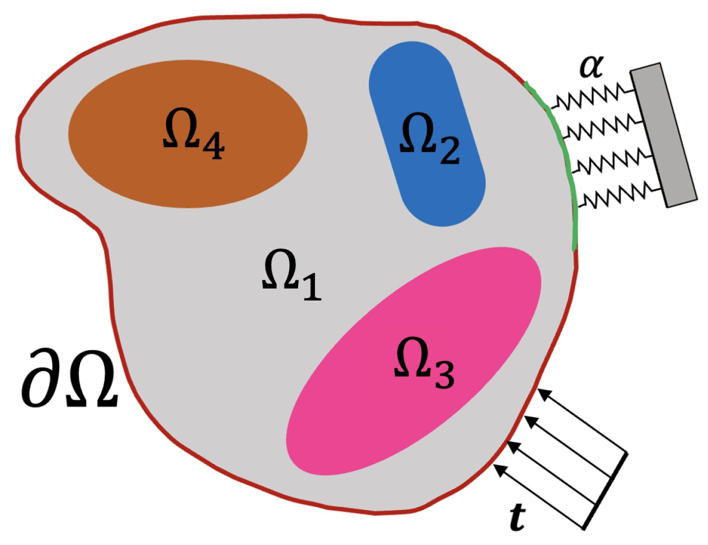
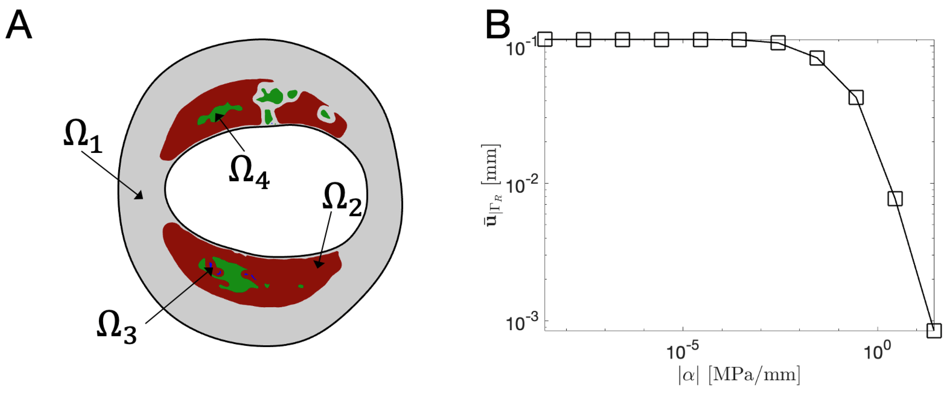
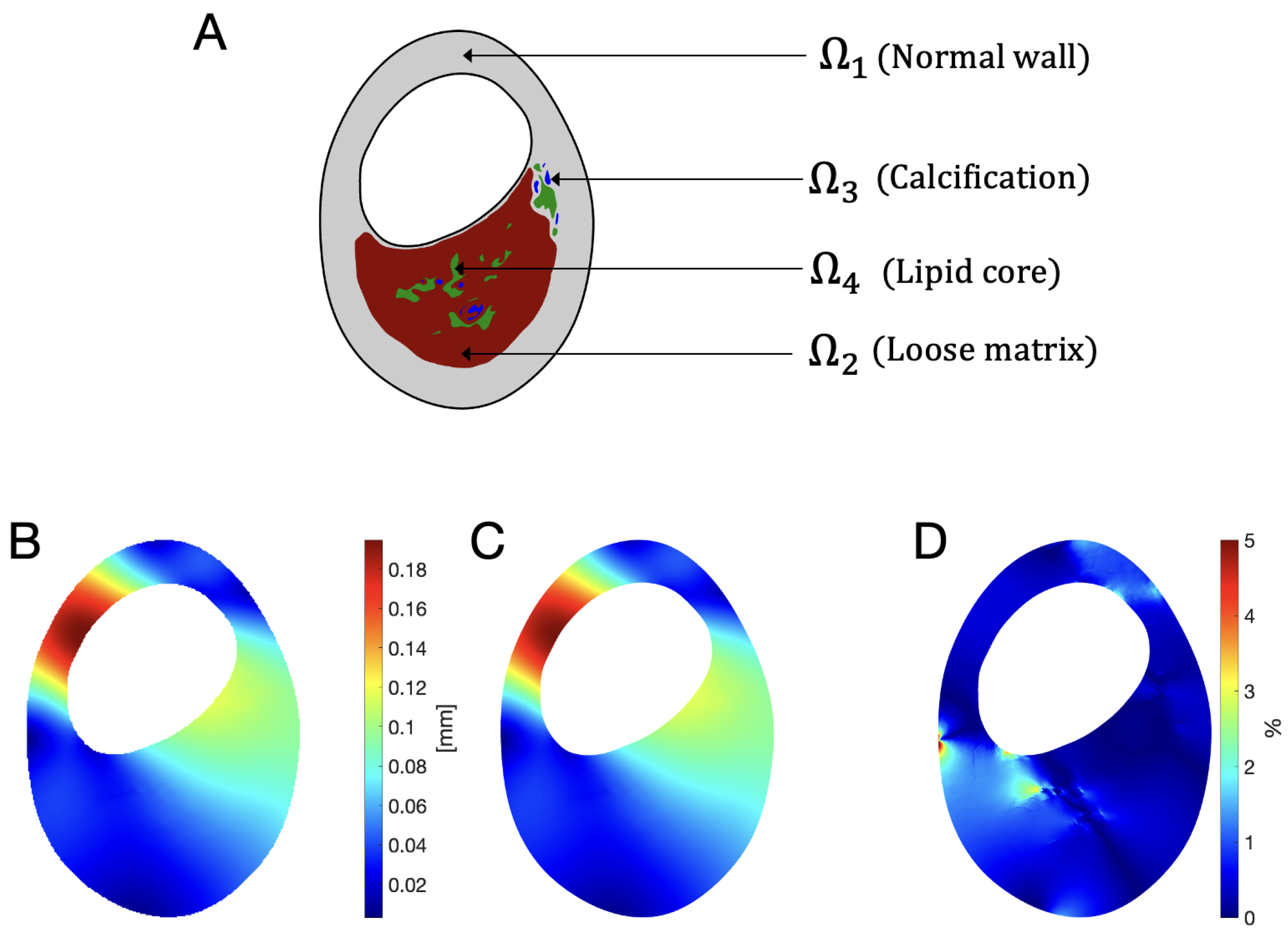
Let the section occupy a region $\Omega \subset {\mathbb{R}}^2$ with boundary $\partial \Omega$. The intrinsic heterogeneity of arterial cross-sections is described by dividing $\Omega$ into different subdomains ${\Omega }_1,{\Omega }_2,\cdots$, corresponding to homogeneous regions having different material properties i.e., normal vessel wall, loose matrix, calcification, and lipid core (see Figure 1). Without body forces, the equilibrium is governed by

$$\nabla ·\sigma \left(\mathbf{u}\right)=\mathbf{0}\mathrm{in}\Omega ,$$

(1)

with boundary conditions

$$\begin{array}{ccc}\hfill \mathit{\sigma }\left(\mathbf{u}\right)·\widehat{\mathbf{n}}& =\mathbf{t}\hfill & \hfill \mathrm{on}{\Gamma }_N,\end{array}$$

(2)

$$\begin{array}{ccc}\hfill \mathit{\sigma }\left(\mathbf{u}\right)·\widehat{\mathbf{n}}& =\alpha \mathbf{u}(\alpha <0)\hfill & \hfill \mathrm{on}{\Gamma }_R,\end{array}$$

(3)

where $\mathit{\sigma }$ is the Cauchy stress tensor and $\mathbf{u}$ is the displacement field; $\mathbf{t}$ is the surface traction, $\alpha$ is the elastic bed coefficient, and $\widehat{\mathbf{n}}$ is the outward unit normal to the boundary. Equation (3) represents the Robin boundary condition, physically corresponding to an elastic bed condition, simulating the surrounding tissue of the artery. The Neumann and elastic bed boundaries cover the whole boundary, i.e., $\partial \Omega ={\Gamma }_N\cup {\Gamma }_R$.

The weak form of Problem 1 (physically corresponding to the principle of virtual work) reads: find $\mathbf{u}\in {\left[{\mathcal{H}}^1(\Omega )\right]}^2$ such that

$${\int }_{\Omega }\mathit{\sigma }\left(\mathbf{u}\right):\epsilon \left(\mathbf{v}\right)\mathrm{d}\Omega -{\int }_{{\Gamma }_R}\alpha \mathbf{u}·\mathbf{v}\mathrm{d}\Gamma ={\int }_{{\Gamma }_N}\mathbf{t}·\mathbf{v}\mathrm{d}\Gamma ,$$

(4)

for all $\mathbf{v}\in {\left[{\mathcal{H}}^1(\Omega )\right]}^2$. ${\mathcal{H}}^1(\Omega )$ is the Sobolev space of order 1 on $\Omega$; refer to [40] for details. Note that the test function $\mathbf{v}$ is also seen as a virtual infinitesimal displacement (a perturbation from the equilibrium configuration of the body) consistent with the imposed boundary displacements, and $\epsilon \left(\mathbf{v}\right)=1/2(\nabla \mathbf{v}+\nabla {\mathbf{v}}^{\top })$. The elastic bed BC (3) is an alternative to the standard practice of suppressing rigid-body motions by prescribing displacements at some arbitrarily selected points. As shown in the following, enforcing an isostatic scheme by prescribing point displacements and elastic bed BC produce similar results. We advocate the latter because the elastic bed BC includes physical information about the surrounding medium and does not require selecting arbitrary points to prescribe displacements. This is crucial for model order reduction, where one has to perform operations with the solutions of different configurations, and hence, they need to be comparable.

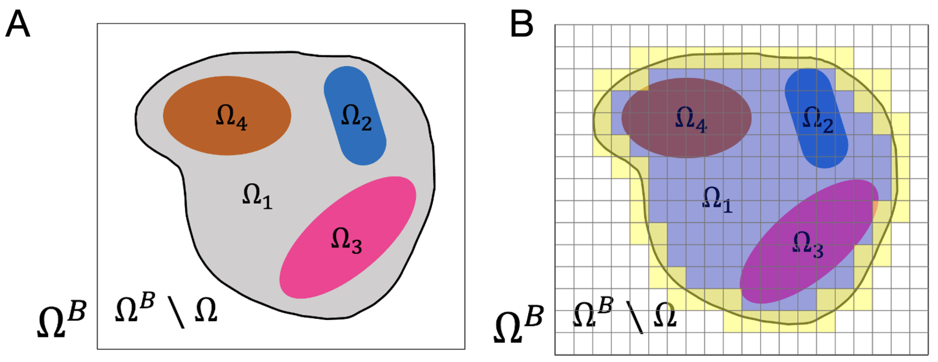
2.2. Level Set Description of the Domain and Subdomains

As introduced previously, the domain $\Omega$ is divided into n subdomains ${\Omega }_i$, $i=1,\cdots ,n$. The n subdomains cover $\Omega$, that is

$$\Omega =\bigcup _{k=1}^n{\Omega }_k.$$

(5)

Level set functions implicitly describe the geometry of $\Omega$ and its subdomains in a unique framework. A background domain ${\Omega }^{\mathrm{B}}$, having a simple geometry (here rectangle or square shape), is introduced to accommodate all possible instances of $\Omega$, resulting in $\Omega \subset {\Omega }^{\mathrm{B}}$; see Figure 2A.

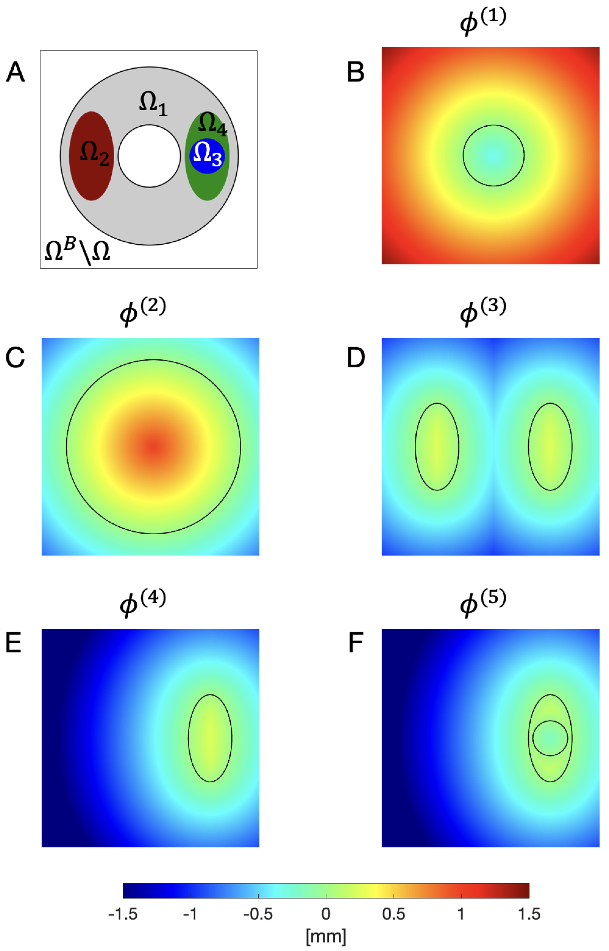
A standard level set to describe $\Omega$ in ${\Omega }^{\mathrm{B}}$ is a continuous function $\varphi$ taking values in ${\Omega }^{\mathrm{B}}$ such that $\varphi \left(\mathbf{x}\right)>0$ for $\mathbf{x}\in \Omega$ and negative elsewhere. Thus, $\varphi \left(\mathbf{x}\right)=0$ for $\mathbf{x}\in \partial \Omega$. Typically, $\varphi$ is a signed distance to $\partial \Omega$ [41,42]. For a configuration such as the one in Figure 3, with two non-connected parts of the boundary, ${\Gamma }_N$ and ${\Gamma }_R$, it is convenient to describe $\Omega$ using two level sets to distinguish between the two. Thus, $\Omega$ is identified with ${\varphi }^{\left(1\right)}$ and ${\varphi }^{\left(2\right)}$ such that: ${\varphi }^{\left(1\right)}\left(\mathbf{x}\right)=0$ on ${\Gamma }_N$, and ${\varphi }^{\left(2\right)}\left(\mathbf{x}\right)=0$ on ${\Gamma }_R$. Both level sets are positive in $\Omega$; see Figure 3B,C for an illustration. Note that one may recover a standard level set for $\Omega$ by just taking $\varphi ={\varphi }^{\left(1\right)}{\varphi }^{\left(2\right)}$. Then, following the ideas in [43], new level set functions are introduced to describe the n subdomains. Function ${\varphi }^{\left(3\right)}$ provides the information to identify ${\Omega }_1$ and distinguish it from the remainder subdomains. In particular, ${\varphi }^{\left(3\right)}\left(\mathbf{x}\right)>0$ for $\mathbf{x}\in {\bigcup }_{k=2}^n{\Omega }_k$ and is negative elsewhere in $\Omega$ (that is in ${\Omega }_1$). Similarly, ${\varphi }^{\left(4\right)}$ is positive in ${\bigcup }_{k=3}^n{\Omega }_k$ and negative in the remainder, that is in ${\bigcup }_{k=1}^2{\Omega }_k$. The last hierarchical level set needed is ${\varphi }^{(n+1)}$ identifying ${\Omega }_{n-1}$ because then ${\Omega }_n$ is precisely the remainder (${\varphi }^{(n+1)}>0$). The values of ${\varphi }^{\left(k\right)}$ with $k=3,\cdots ,n+1$ outside $\Omega$ are not relevant. This is consistent with the hierarchical character of this approach. A visualization of the hierarchical level sets is illustrated in the panels of Figure 3 and summarized in

Table 1. Level set-based criteria to classify a point $\mathbf{x}$ in $\Omega$ and its subdomains.

Condition	Classification
${\varphi }^{\left(1\right)}>0$ and ${\varphi }^{\left(2\right)}>0$	$\mathbf{x}\in \Omega$
${\varphi }^{\left(1\right)}>0$ and ${\varphi }^{\left(2\right)}>0$ and ${\varphi }^{\left(3\right)}<0$	$\mathbf{x}\in {\Omega }_1$
${\varphi }^{\left(1\right)}>0$ and ${\varphi }^{\left(2\right)}>0$ and ${\varphi }^{\left(3\right)}>0$ and ${\varphi }^{\left(4\right)}<0$	$\mathbf{x}\in {\Omega }_2$
${\varphi }^{\left(1\right)}>0$ and ${\varphi }^{\left(2\right)}>0$ and ${\varphi }^{\left(3\right)}>0$ and ${\varphi }^{\left(4\right)}>0$ and ${\varphi }^{\left(5\right)}<0$	$\mathbf{x}\in {\Omega }_3$
${\varphi }^{\left(1\right)}>0$ and ${\varphi }^{\left(2\right)}>0$ and ${\varphi }^{\left(5\right)}>0$	$\mathbf{x}\in {\Omega }_4$

.

The approach described above is similar to the front-tracking method used to simulate multiphase flow with a fixed grid for the flow [44], with the difference that the front does not change with time, and therefore, the level set is computed only once at the beginning of the analysis.

2.3. Discretization of the Level Set Functions in a Background Mesh

With a finite element (FE) discretization of ${\Omega }^{\mathrm{B}}$ (see Figure 2), the level set approach is implemented. A tessellation ${\mathcal{T}}_h$ of ${\Omega }^{\mathrm{B}}$ consisting of $n_{\mathrm{e}}$ elements $T_e$, $e=1,2,\cdots ,n_{\mathrm{e}}$ (h stands for the characteristic size of the elements) is introduced, such that ${\Omega }^{\mathrm{B}}={\bigcup }_{e=1}^{n_{\mathrm{e}}}{T}_e$. The number of nodes in the mesh is denoted by $n_{\mathrm{p}}$ and the corresponding shape functions are denoted by $N_i\left(\mathbf{x}\right)$, for $i=1,2,\cdots ,n_{\mathrm{p}}$ c[cyan]. Thus, each level set ${\varphi }^{\left(k\right)}$, $k=1,\dots ,n+1$, is represented in the background mesh as

$${\varphi }^{\left(k\right)}\left(\mathbf{x}\right)\approx \sum _{i=1}^{n_{\mathrm{p}}}{\left[{\mathbf{\Phi }}^k\right]}_i{N}_i\left(\mathbf{x}\right),$$

(6)

with ${\mathrm{\Phi }}^k\in {\mathbb{R}}^{n_{\mathrm{p}}}$ being the vector of nodal values describing ${\varphi }^{\left(k\right)}$. In this framework, $n+1$ vectors in ${\mathbb{R}}^{n_{\mathrm{p}}}$ describe any geometrical configuration. This standardized representation allows for dimensionality reduction given the variance in the population of input samples (each corresponding to a different patient). To ease the task of the machine learning algorithms to be used in dimensionality reduction, standard geometric normalizations are performed previously to store the information in the discrete level set format. For instance, all samples are centered (their barycenter is translated to the origin of coordinates) and rotated such that the principal axes of inertia are parallel to the coordinate axes.

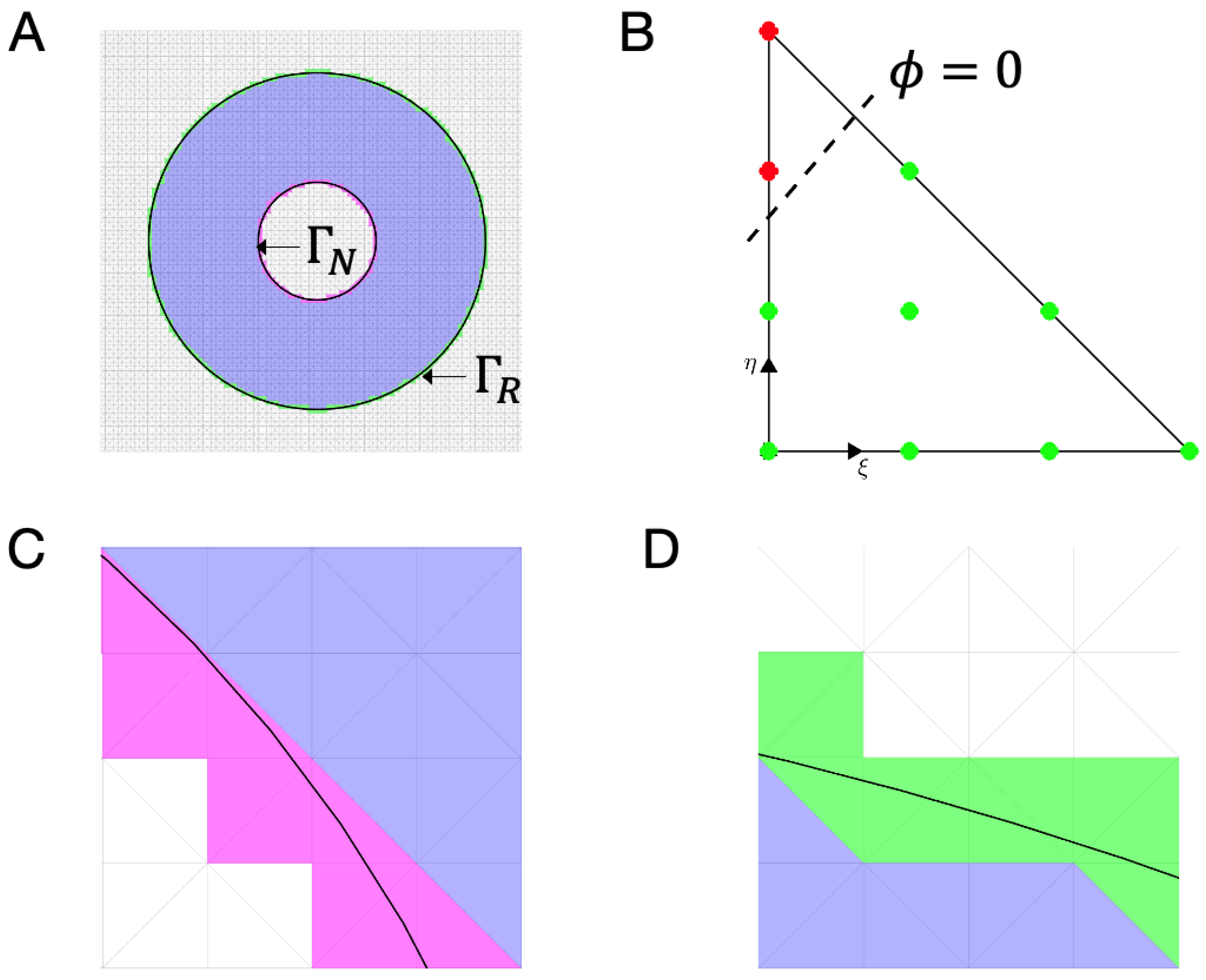
2.4. Unfitted Approach: Solving the Problem in the Background Mesh

The framework for approximating the level set over ${\mathcal{T}}_h\left({\Omega }^{\mathrm{B}}\right)$ just described is used to solve the original problem (4) using an unfitted approach based on the ideas of the Immersed Boundary Method (IBM). Thus, the displacement field $\mathbf{u}\left(\mathbf{x}\right)$ is approximated in the background mesh using a standard FE approximation, namely

$$\mathbf{u}\left(\mathbf{x}\right)\approx \sum _{i=1}^{n_{\mathrm{p}}}{\mathbf{U}}_i{N}_i\left(\mathbf{x}\right),$$

(7)

with ${\mathbf{U}}_i\in {\mathbb{R}}^2$ being the displacement vector in node i. All vectors ${\mathbf{U}}_i$, $i=1,2,\cdots ,n_{\mathrm{p}}$, are collected in the standard vector of nodal displacements $\mathbf{U}\in {\mathbb{R}}^{2n_{\mathrm{p}}}$. Using the Galerkin strategy to solve Equation (4) results in a linear system of equations for $\mathbf{U}$:

$$\left[\mathbf{K}+\mathbf{M}\right]\mathbf{U}=\mathbf{F},$$

(8)

where matrices $\mathbf{K}$ and $\mathbf{M}$ in ${\mathbb{R}}^{2n_{\mathrm{p}}\times 2n_{\mathrm{p}}}$ are the discrete counterparts of the two bilinear forms in the left-hand side of Equation (4) and $\mathbf{F}\in {\mathbb{R}}^{2n_{\mathrm{p}}}$ is the discretization of the linear form in the right-hand side.

Note that a node i in the mesh is represented by the degrees of freedom $\ell =2(i-1)+1$ and $\ell +1$ in $\mathbf{U}$, and some other node j is represented by $\tilde{\ell }=2(j-1)+1$ and $\tilde{\ell }+1$. Assuming these relations, some illustrative examples of the expressions for the corresponding entries in the matrices and the right-hand-side vector are given below

$${\left[\mathbf{K}\right]}_{\ell \tilde{\ell }}={\int }_{\Omega }\mathit{\sigma }\left(\left[\begin{array}{c}{N}_i\left(\mathbf{x}\right)\\ 0\end{array}\right]\right):\epsilon \left(\left[\begin{array}{c}{N}_j\left(\mathbf{x}\right)\\ 0\end{array}\right]\right)\mathrm{d}\Omega ;{\left[\mathbf{K}\right]}_{\ell ,\tilde{\ell }+1}={\int }_{\Omega }\mathit{\sigma }\left(\left[\begin{array}{c}{N}_i\left(\mathbf{x}\right)\\ 0\end{array}\right]\right):\epsilon \left(\left[\begin{array}{c}0\\ N_j\left(\mathbf{x}\right)\end{array}\right]\right)\mathrm{d}\Omega$$

$${\left[\mathbf{M}\right]}_{\ell \tilde{\ell }}=-{\int }_{{\Gamma }_R}\alpha \left[\begin{array}{c}{N}_i\left(\mathbf{x}\right)\\ 0\end{array}\right]·\left[\begin{array}{c}{N}_j\left(\mathbf{x}\right)\\ 0\end{array}\right]\mathrm{d}\Gamma ;{\left[\mathbf{M}\right]}_{\ell ,\tilde{\ell }+1}=-{\int }_{{\Gamma }_R}\alpha \left[\begin{array}{c}{N}_i\left(\mathbf{x}\right)\\ 0\end{array}\right]·\left[\begin{array}{c}0\\ N_j\left(\mathbf{x}\right)\end{array}\right]\mathrm{d}\Gamma$$

$${\left[\mathbf{F}\right]}_{\ell }={\int }_{{\Gamma }_N}\mathbf{t}·\left[\begin{array}{c}{N}_i\left(\mathbf{x}\right)\\ 0\end{array}\right]\mathrm{d}\Gamma ;{\left[\mathbf{F}\right]}_{\ell +1}={\int }_{{\Gamma }_N}\mathbf{t}·\left[\begin{array}{c}0\\ N_i\left(\mathbf{x}\right)\end{array}\right]\mathrm{d}\Gamma .$$

Note that all the integrals in the expressions above are defined in $\Omega$, ${\Gamma }_R$, and ${\Gamma }_N$, and not in the background domain ${\Omega }^{\mathrm{B}}$ where the FE functions $N_i\left(\mathbf{x}\right)$ are supported. In particular, evaluating the local contributions (the integrals are restricted to some element $T_e$) requires identifying whether an element intersects ${\Gamma }_R$ or ${\Gamma }_N$. Thus, the main implementation challenge of the unfitted approach is classifying the elements ${\mathcal{T}}_h$ of ${\Omega }^{\mathrm{B}}$ inside $\Omega$, those outside, and those crossed by the interfaces. For a given configuration, the geometrical information is encoded in the level sets, as described in Section 2.2. This allows elaborating a list of the elements in ${\mathcal{T}}_h$ that are completely inside $\Omega$, namely ${\mathcal{I}}_{\Omega }$ such that if $e\in {\mathcal{I}}_{\Omega }$, then $T_e\subset \Omega$. Similarly, lists ${\mathcal{I}}_{{\Gamma }_R}$ and ${\mathcal{I}}_{{\Gamma }_N}$ are such that if $e\in {\mathcal{I}}_{{\Gamma }_R}$ then $T_e\bigcap {\Gamma }_R\ne \varnothing$, and if $e\in {\mathcal{I}}_{{\Gamma }_N}$ then $T_e\bigcap {\Gamma }_N\ne \varnothing$. Figure 4 shows an example of such classification. The elements indexed in these three lists are active, meaning that they play a role in the solution for the configuration described by the level sets. Thus, $T_e$ is said to be active if $e\in {\mathcal{I}}_{\Omega }\bigcup {\mathcal{I}}_{{\Gamma }_R}\bigcup {\mathcal{I}}_{{\Gamma }_N}$. Accordingly, all the nodes belonging to active elements are active nodes since the corresponding degrees of freedom are the unknowns of (8) (the non-active nodes are to be eliminated from the system).

The computation of the elementary contributions to the stiffness matrix $\mathbf{K}$ is standard for the elements completely inside $T_e$ for $e\in {\mathcal{I}}_{\Omega }$ (violet elements in Figure 4A). The only particular feature to be accounted for is that the material properties of each Gauss point in the numerical quadrature belong to a subdomain ${\Omega }_k$. With the values of the level sets interpolated at the Gauss point, following the classification described in Table 1, the material properties are quickly recovered. Note that for the example shown in Figure 4A, only two level sets, ${\varphi }^{\left(1\right)}$ and ${\varphi }^{\left(2\right)}$, are required. In the elements crossed by the interfaces ${\Gamma }_R$ and ${\Gamma }_N$, the integration has to exclude the part of the domain outside $\Omega$. There, a more refined quadrature is used, and null material properties are assigned to the integration points outside $\Omega$. A closed quadrature is preferred to avoid accounting for integration points inside elements with a small portion inside $\Omega$. These geometric checks are performed by setting a tolerance and considering that the distance to the interface is zero when it is below this value. Computing elementary contributions to matrix $\mathbf{M}$ and vector $\mathbf{F}$ requires integrating within the portion of ${\Gamma }_R$ or ${\Gamma }_N$ in the element $T_e$. Thus, for $e\in {\mathcal{I}}_{{\Gamma }_N}$, $T_e$ intersects ${\Gamma }_N$ and contributes to $\mathbf{F}$. Analogously, for $e\in {\mathcal{I}}_{{\Gamma }_R}$, $T_e$ intersects ${\Gamma }_R$ and contributes to $\mathbf{M}$.

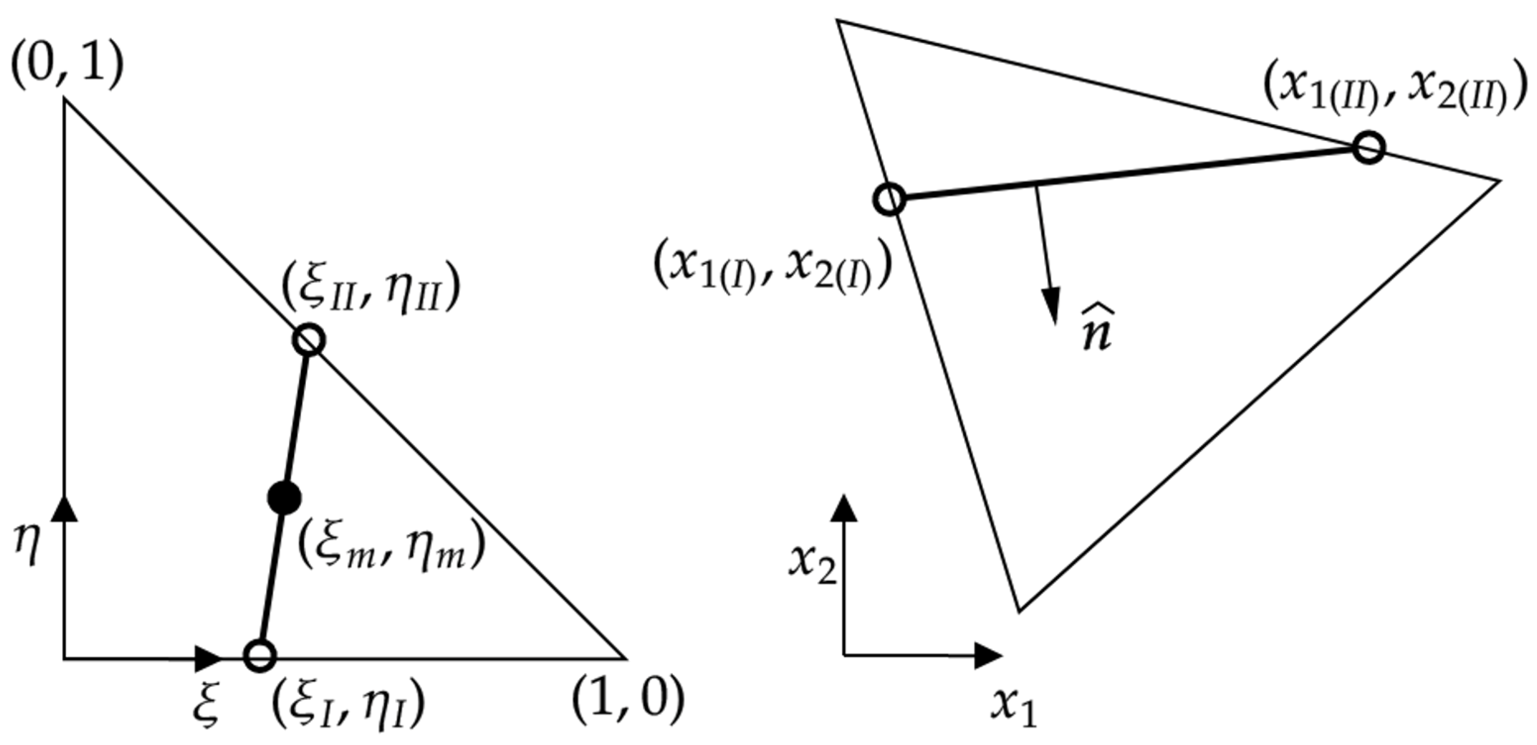
For $e\in {\mathcal{I}}_{{\Gamma }_N}$, the elementary contribution from element $T_e$ to $\mathbf{F}$ requires computing

$${\int }_{{\Gamma }_N\bigcap T_e}{\left[\mathbf{t}\right]}_1{N}_i\left(\mathbf{x}\right)\mathrm{d}\Gamma \mathrm{and}{\int }_{{\Gamma }_N\bigcap T_e}{\left[\mathbf{t}\right]}_2{N}_i\left(\mathbf{x}\right)\mathrm{d}\Gamma ,$$

(9)

for all the nodes i in element $T_e$. If the load corresponds to a pressure p applied in the internal wall, then $\mathbf{t}=-p\widehat{\mathbf{n}}$, recalling that $\widehat{\mathbf{n}}={\left[n_1{n}_2\right]}^{\top }$ is the outward unit normal. Thus, ${\left[\mathbf{t}\right]}_1=-p{n}_1$ and ${\left[\mathbf{t}\right]}_2=-p{n}_2$. This integral, as it is standard in the FE practice, is computed in a reference element (for linear triangles, it is handy using the triangle with vertices $(0,0)$, $(1,0)$ and $(0,1)$, see Figure 5), where the shape functions are defined (and available in their analytical expressions) in terms of the reference coordinates $(\xi ,\eta )$, namely ${\widehat{N}}_{\left(i\right)}(\xi ,\eta )$, for $\left(i\right)=1,2,3$. Mesh connectivity provides the link between the local numbering of the node inside the element, $\left(i\right)$ (from 1 to 3 in the case of linear triangles), and the global numbering i (from 1 to $n_{\mathrm{p}}$). Since $T_e$ is crossed by ${\Gamma }_N$, it is important to identify the entry and exit points in the element, that is the points $\{P_I,P_{II}\}={\Gamma }_N\bigcap \partial T_e$; see Figure 5. This task is performed while identifying the elements in ${\mathcal{I}}_{{\Gamma }_N}$, and it is straightforward after the nodal values of ${\varphi }^{\left(1\right)}$. Recall that ${\varphi }^{\left(1\right)}\left(\mathbf{x}\right)=0$ for $\mathbf{x}\in {\Gamma }_N$. Same rationale works for ${\Gamma }_R$, using ${\varphi }^{\left(2\right)}$. A quadrature is required to integrate along the segment $P_I{P}_{II}$ (a portion of ${\Gamma }_N$). Here, a Simpson quadrature is adopted and involves computing the values of the function to be integrated on the endpoints of the interval and in the midpoint, $P_{\mathrm{m}}$; see Figure 5. The general expression for Simpson quadrature to approximate the integral of some function $\psi$ reads:

$${\int }_{P_I}^{P_{II}}\psi \mathrm{d}\Gamma \approx \frac{|P_I{P}_{II}|}{6}(\psi \left(P_I\right)+4\psi \left(P_{\mathrm{m}}\right)+\psi \left(P_{II}\right)),$$

(10)

where $|P_I{P}_{II}|$ is the length of the interval $P_I{P}_{II}$. Thus, computing the terms in (9) requires obtaining the values of $N_i$ in the three points $P_I$, $P_{II}$ and $P_{\mathrm{m}}$. These values are easily obtained after their coordinates in the reference element, $({\xi }_I,{\eta }_I)$, $({\xi }_{II},{\eta }_{II})$ and $({\xi }_{\mathrm{m}},{\eta }_{\mathrm{m}})$. Then, it suffices using the quadrature given in (10) for $\psi \left(\mathbf{x}\right)=-p{n}_1{N}_i\left(\mathbf{x}\right)$ and $\psi \left(\mathbf{x}\right)=-p{n}_2{N}_i\left(\mathbf{x}\right)$ to obtain the horizontal and vertical components of the nodal forces (on node i from element e).

Similarly, for $e\in {\mathcal{I}}_{{\Gamma }_R}$, the elementary contribution from $T_e$ to $\mathbf{M}$ requires computing terms of the form

$${\int }_{{\Gamma }_R\bigcap T_e}\alpha N_i\left(\mathbf{x}\right)N_j\left(\mathbf{x}\right)\mathrm{d}\Gamma .$$

(11)

This is achieved by taking $\psi \left(\mathbf{x}\right)=\alpha N_i\left(\mathbf{x}\right)N_j\left(\mathbf{x}\right)$ and using the quadrature (10) accordingly. In the unfitted solution, the degrees of freedom corresponding to nodes that do not belong to any of the active elements (those with index e in $\bigcup {\mathcal{I}}_{{\Gamma }_R}\bigcup {\mathcal{I}}_{{\Gamma }_N}$) must be removed from system (8).

The number of active nodes (that is the number of nodes in the active elements) is denoted by $n_{\mathrm{act}}$ and indicates the measure of the size of the system to be solved. Note that in conformal FE, $n_{\mathrm{act}}$ is the number of nodes in the mesh. On the other hand, in an unfitted approach, $n_{\mathrm{act}}<n_{\mathrm{p}}$.

The proposed methodology has been entirely implemented in Matlab R2022b, The MathWorks Inc, and executed in a 3.2 GHz Apple M1 with 8 GB RAM.

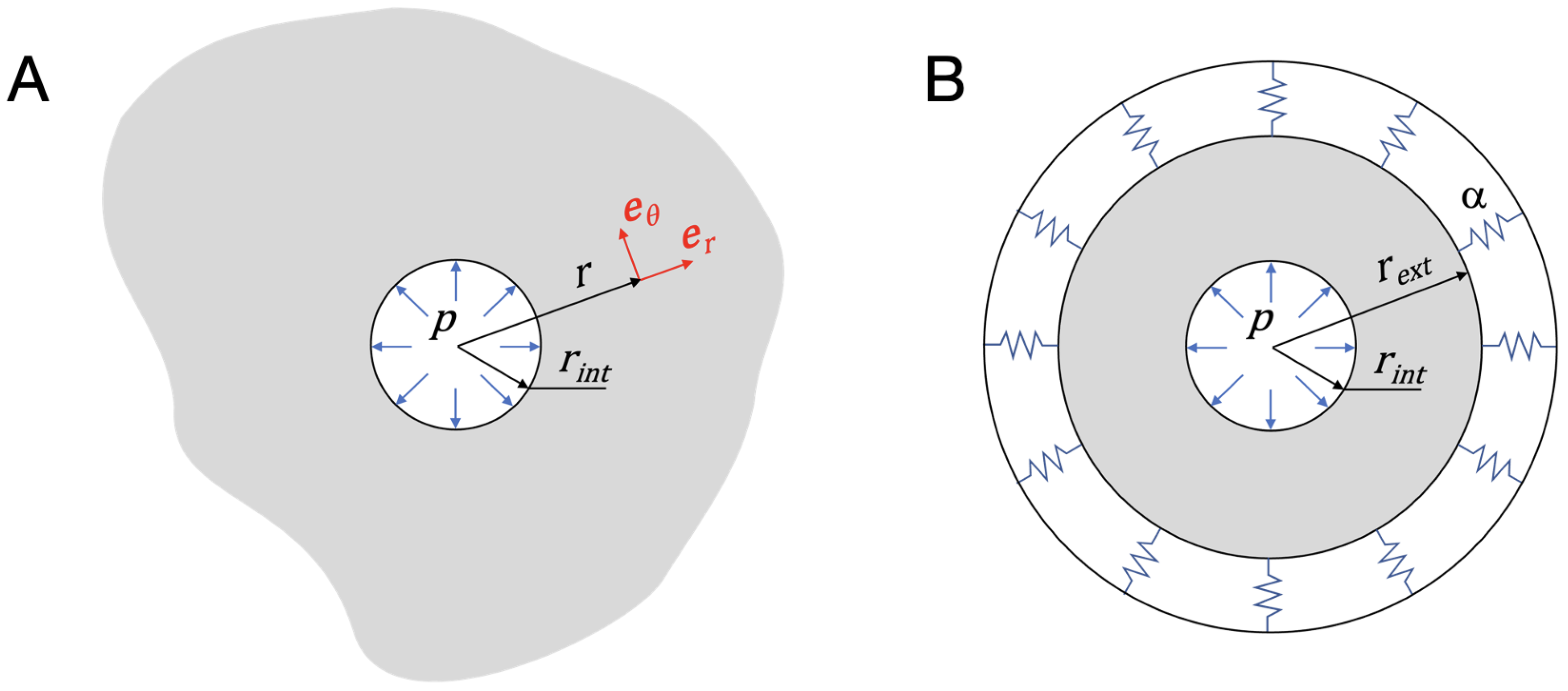
2.5. Validating the Methodolgy

The solution of an infinite linear elastic solid with a cylindrical cavity of radius $r_{int}$ subjected to internal pressure p (Figure 6A) is considered.

Assuming cylindrical coordinates, the analytical solution of the problem is [46]

$$u_r=p\frac{r_{int}^2}{2\mu r},u_{\theta }=u_z=0,$$

(12)

where $\mu =\mu (E,v)$ is the shear modulus of the material, E and $\nu$ are its Young’s modulus and Poisson ratio, respectively, and $r\ge r_{int}$ is the radial coordinate. The strain and stress fields are obtained with the constitutive equations for a linear elastic solid as

$$\begin{array}{cc}\hfill {\epsilon }_{rr}& =\frac{\partial u_r}{\partial r}=-\frac{p}{2\mu }{\left(\frac{r_{int}}{r}\right)}^2,\hfill \end{array}$$

(13)

$$\begin{array}{cc}\hfill {\epsilon }_{\theta \theta }& =\frac{u_r}{r}=\frac{p}{2\mu }{\left(\frac{r_{int}}{r}\right)}^2,\hfill \end{array}$$

(14)

$$\begin{array}{cc}\hfill {\epsilon }_{zz}& =0,\hfill \end{array}$$

(15)

$$\begin{array}{cc}\hfill {\sigma }_{rr}& =-p{\left(\frac{r_{int}}{r}\right)}^2,\hfill \end{array}$$

(16)

$$\begin{array}{cc}\hfill {\sigma }_{\theta \theta }& =p{\left(\frac{r_{int}}{r}\right)}^2,\hfill \end{array}$$

(17)

$$\begin{array}{cc}\hfill {\sigma }_{zz}& =0.\hfill \end{array}$$

(18)

This problem is equivalent to that of an infinite cylinder of internal radius $r_{int}$ and external radius, $r_{ext}$, subjected to internal pressure, p (applied at $r=r_{int}$), and elastic bed BC on $r=r_{ext}$ (see Figure 6B), with the ballast coefficient $\alpha$ given as

$$\alpha =-\frac{2\mu }{r_{ext}},$$

(19)

obtained from (3) together with (12), and (16)–(18).

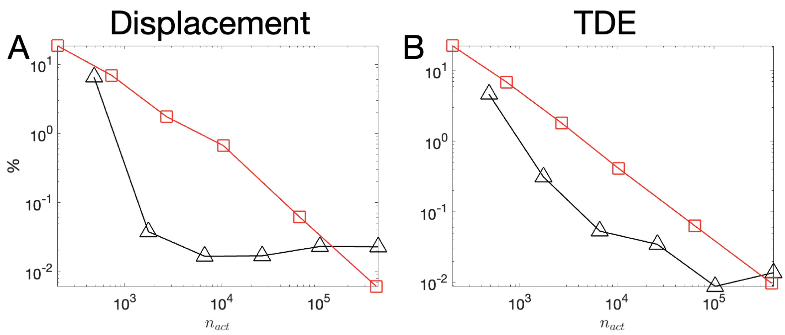
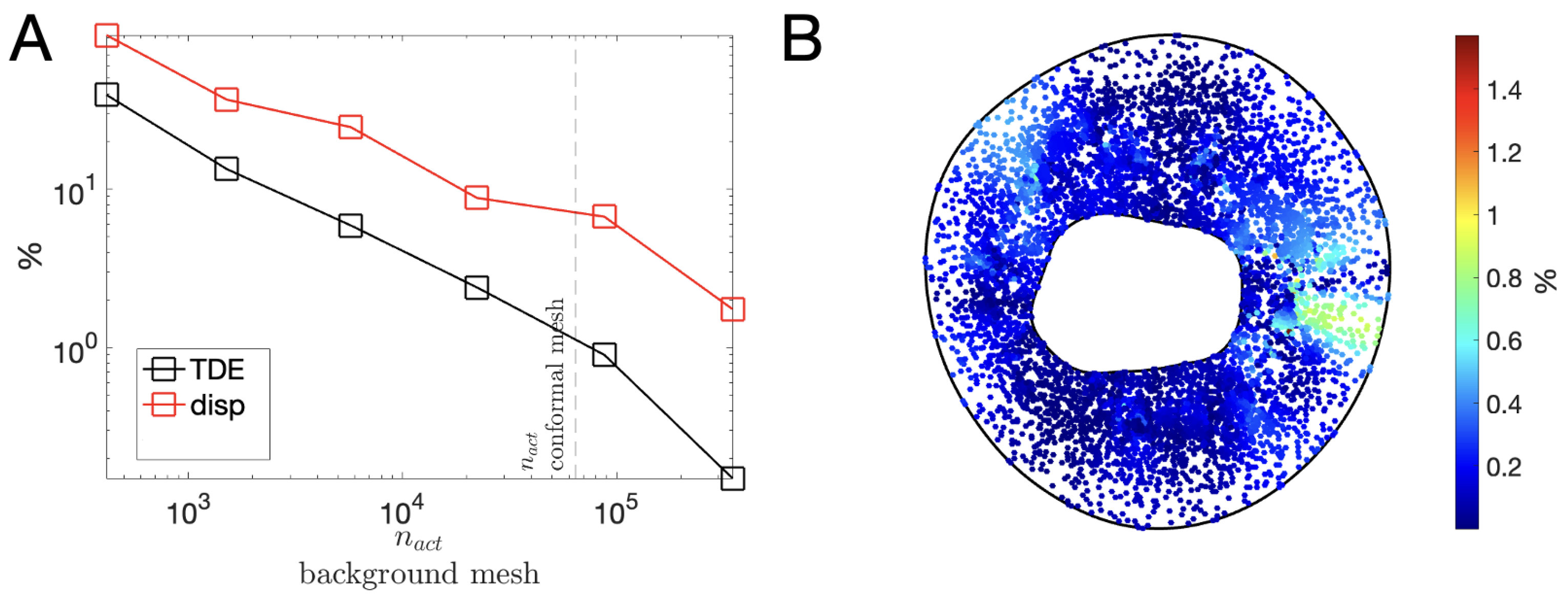
With this problem at hand, the accuracy of the methodology is quantified in terms of local and global quantities. The displacement field is a local quantity of accuracy, and the total deformation energy (TDE) is used as a global metric to assess the convergence for the numerical solution. The TDE for the infinite cylinder in Figure 6B is given by

$$\begin{array}{cc}\hfill \mathrm{TDE}& =\frac{1}{2}{\int }_0^{2\pi }{\int }_{r_{int}}^{r_{ext}}({\sigma }_{rr}{\epsilon }_{rr}+{\sigma }_{\theta \theta }{\epsilon }_{\theta \theta })r\mathrm{d}r\mathrm{d}\theta =\hfill \\ \hfill & =\pi {\int }_{r_{int}}^{r_{ext}}\left[\left(\frac{p^2{r}_{int}^4}{2\mu r^4}\right)+\left(\frac{p^2{r}_{int}^4}{2\mu r^4}\right)\right]r\mathrm{d}r=\frac{\pi p^2{r}_{int}^4}{2\mu }\left(\frac{1}{r_{int}^2}-\frac{1}{r_{ext}^2}\right)>0.\hfill \end{array}$$

(20)

Note that (20) only accounts for the elastic energy stored in the cylinder and not in the elastic bed. Numerically, the TDE is calculated as

$${\mathrm{TDE}}_{\mathrm{num}}=\frac{1}{2}{\mathbf{U}}^{\top }\mathbf{K}\mathbf{U},$$

(21)

where $\mathbf{U}$ corresponds to the displacement vector of the active nodes in the background mesh, and $\mathbf{K}$ is the stiffness matrix associated with the active elements in the background mesh.

3. Results

3.1. Covergence Analysis

To show the accuracy of the methodology, problem (1) is solved using the proposed Immersed Boundary Robin-based (IBR) model, on the idealized geometry domain of Figure 6B, for an internal pressure of $p={10}^{-2}$ MPa. Consequently, the analytical solution of the problem is calculated for the infinite solid with a cylindrical cavity at $r_{int}$ (Figure 6A). Recall that, to make equivalent both the analytical results with the Robin-based approach, the ballast coefficient $\alpha$ of Equation( 19) is used. The different model parameters used for this study are reported in

Table 2. Model parameters: Young’s modulus E, Poisson ratio $\nu$ and the ballast coefficient $\alpha$.

E (MPa)	$\mathit{\nu }$	$\mathit{\alpha }$ (MPa/mm)	${\mathit{r}}_{\mathit{int}}$ (mm)	${\mathit{r}}_{\mathit{ext}}$ (mm)
$7.3313\times {10}^{-1}$	$0.475$	$-1.2426\times {10}^{-1}$	$1.5$	4

.

Figure 7A represents the relative error of the displacements at an arbitrary point with radius $r\in \left\{r_{int},r_{ext}\right\}$ (compared to the analytical solution obtained using Equation (12)) of both the proposed Immersed Boundary Robin-based approach (in black) and the classical FE approach in red (which is calculated for completeness in the analysis).

In addition, recalling Equations (20) and (21), the relative error (with respect to the analytical value) of the total deformation energy (TDE) is also calculated for both the IBR and the classical FE models and represented in Figure 7B in black and red, respectively. It is worth noting the convergence behavior by increasing the number of active nodes, which means refining the conformal mesh for the classical FE approach and the unfitted background mesh for the IBR solution; the solution improves faster for a smaller number of active nodes using our IBR methodology until a stabilization plateau, where the relative error of TDE stagnates at a value close to ${10}^{-4}$. This is likely due to truncation errors affecting quantities computed in the unfitted procedure, mainly integrals in elements divided by boundaries. This level of accuracy is perfectly acceptable in this type of model.

3.2. Elastic Bed Coeficient $\alpha$: Sensitivity Analysis

As mentioned in Section 2.1, the elastic bed coefficient $\alpha$ represents an elastic bed boundary condition that simulates the interaction of the body with its surroundings. Therefore, it is also possible to tune $\alpha$ so that it only avoids rigid body motions (and not influencing nodal displacements and stresses). For this study, Figure 8A shows a realistic arterial section where the proposed $\alpha$ analysis is applied under an internal pressure $p=2.6267\times {10}^{-2}$ MPa. Homogeneous linear elastic material properties were used, being the material parameters reported in

Table 3. Material parameters of the piece-wise homogeneous domain $\Omega ={\bigcup }_{k=1}^4{\Omega }_k$ (i.e., normal vessel wall, loose matrix, calcification, and lipid core), E (Young’s modulus) and $\nu$ (Poisson ratio).

Subdomain	Material	E [MPa]	$\mathit{\nu }$	Ref.
${\Omega }_1$	Normal vessel-wall	$0.73$	$0.475$	[22]
${\Omega }_2$	Loose matrix	$0.431$	$0.475$	[22]
${\Omega }_3$	Calcification	$1.5\times {10}^4$	$0.3$	[23]
${\Omega }_4$	Lipid core	$1.8841\times {10}^{-1}$	$0.475$	[22]

.

According to this, the graph in Figure 8B shows that by decreasing the elastic bed coefficient $\alpha$, the average displacements at the external boundary (${\overline{\mathbf{u}}}_{|{\Gamma }_R}$) becomes unaffected by the surroundings while eliminating rigid body motion. That is to say, the left part of the graph corresponds to the limit value of a floating object with no surrounding stiffness: the small values of $\alpha$ do only suppress rigid-body modes. The limit case for large values of $\alpha$ has zero displacements in the external boundary, as it is reflected in the plot.

3.3. Characteristic Length h of the Background Mesh ${\mathcal{T}}_h\left({\Omega }^{\mathrm{B}}\right)$: Sensitivity Analysis

A relevant parameter in the IBR methodology is the characteristic length h of the background mesh. It is strictly related to the number of active nodes ($n_{act}$) by inverse proportionality, meaning the smaller the h value, the greater the $n_{act}$ value. It is possible to verify how the IBR solution, in terms of displacements and TDE, converges to those obtained with the classical FE method using a very fine mesh. For this, six background meshes ${\mathcal{T}}_{h\left(i\right)}\left({\Omega }^{\mathrm{B}}\right)$$i=1,\cdots ,6$ are used with a decreasing value of h as i increases.

Figure 9 shows the results of such analysis for the section depicted in Figure 8. Figure 9A reports the error for both displacements and TDE associated with the six background meshes with respect to the conformal mesh solution, where it is shown the clear error decreases by increasing the number of active nodes. As an example, Figure 9B shows a plot of the local displacements difference error associated with the finest background mesh developed for this analysis.

Table 4. Results of the sensitivity analysis about the characteristic length h for TDE and displacement magnitude. From mesh 5, there are more active nodes ($n_{act}$) in the background than nodes in the conformal mesh ($n_{act}\mathrm{conformal}\mathrm{mesh}=\mathrm{64,552}$).

Mesh #	${\mathit{n}}_{\mathbf{act}}$	Diff. for TDE	max Diff. for Displacement Magnitude
1	414	$39.3$%	$93.6$%
2	1507	$13.4$%	$36.7$%
3	5734	$5.9$%	$24.6$%
4	$22,270$	$2.4$%	$8.8$%
5	$87,776$	$0.9$%	$6.7$%
6	$348,550$	$0.15$%	$1.75$%

shows the maximum differences in TDE and the displacement magnitude for the different background meshes considered in the analysis.

3.4. Realistic Immersed Boundary Robin-Based approach

Figure 10 shows a comparison between the IBR methods and the classical FE approach for a realistic coronary section, described in Figure 10A, subjected to an internal pressure of $p={10}^{-2}$ MPa. The model parameters used for this study are shown in

Table 5. Background mesh ${\mathcal{T}}_h\left({\Omega }^{\mathrm{B}}\right)$ and conformal mesh ${\mathcal{T}}_h(\Omega )$ parameters.

	${\mathit{n}}_{\mathbf{act}}$	Active Elements	$\mathit{\alpha }$ (MPa/mm)
${\mathcal{T}}_h\left({\Omega }^{\mathrm{B}}\right)$	42,397	83,378	$-1.7736\times {10}^{-4}$
${\mathcal{T}}_h(\Omega )$	47,505	94,210

, being the material properties reported in Table 3.

Figure 10B shows the displacement field obtained with the proposed Immersed Boundary method (obtaining a total deformation energy TDE = $6.8226\times {10}^{-3}$), while Figure 10C corresponds to the solution obtained with the classical FE method (TDE = $6.8248\times {10}^{-3}$). Differences in the total deformation energy are found to be less than 0.05%, with a maximum difference in the displacement magnitude of less than 5% (Figure 10D), being an average error of less than 0.5% in the section. Figure 11A,B show the distribution of the Von Misses stress obtained for both methodologies, IBR method, and the classical FE method, respectively, showing a highly similar stress distribution.

4. Discussion

Computational engineering is considered a potentially powerful tool for biomedical sciences. Nevertheless, one of the most critical drawbacks is the time required to develop credible and accurate numerical solutions where fast patient-specific decision making is necessary, i.e., in the vascular biomechanics field. Advancing in this direction, the article presents a novel formulation that combines hierarchical level sets (from a 2D arterial segmentation) with an Immerse Boundary-Robin-based (IBR) formulation to obtain stress and strain distributions in arterial sections under physiological conditions of blood pressure.

The hierarchical level sets allow us to describe the arterial geometries (segmentations), including internal materials distributions (healthy tissue, lipid core, calcified core, among others) and their properties in a highly standardized format. The use of level sets also allows for using a single background mesh to simulate different patient-specific arterial segmentations, all with the same number of degrees of freedom, thus avoiding the preprocessing stages for developing a different conformal finite element mesh per geometry. Furthermore, having the same number of degrees of freedom allows developing so-called “a posteri” reduced-order models (ROMs) or dimensionality reduction methodologies toward fast (even real-time) simulations. It is worth mentioning that despite vascular tissues exhibiting nonlinear behavior, here, a simple linear elastic model is adopted to demonstrate the performance of the proposed approach in the benchmarks selected. Note that the proposed formulation is straightforwardly generalizable to any type of material model. As expected, the accuracy of the IBR depends on the size of the background mesh relative to the minimum size of the heterogeneity. One way to overcome this limitation is to consider an adaptive background mesh with a higher element density near the heterogeneities.

Using the elastic bed boundary conditions (instead of classical Dirichlet) allows us to effectively remove the rigid body motion without altering the natural deformation of the arterial section due to the internal pressure. However, this boundary condition may also be used to account for the effect of the surrounding tissue on the artery in case the information is known. For instance, a uniform ballast coefficient, $\alpha$, may represent an artery entirely surrounded by tissue as could be the case of the middle cerebral artery or a penetrating myocardial coronary artery. It could also be used to model a partially surrounded artery by specifying a non-uniform ballast coefficient along the external contour of the section. The results obtained with the proposed methodology in terms of displacement and stress fields were very similar compared to those imposing isostatic Dirichlet-type boundary conditions, which are widely accepted in the scientific community. To the best knowledge of the authors, this is the first attempt to propose Immersed Boundary methods with elastic bed boundary conditions for this type of simulation, showing the strong potential of the methodology for biomechanical applications.