
Hamilton–Jacobi Inequality Adaptive Robust Learning Tracking Controller of Wearable Robotic Knee System


Abstract
:1. Introduction
- By considering model errors and external disturbances, the Lagrange theory is used to derive the dynamics equations of the WRK system.
- A control input is developed for the WRK system from feedback action, which determines the difference between the current knee angle value and the required angle value.
- The HJI-based gain technique is established to prove the stability of the WRK’s control system and to enable control motion solutions.
- By using RBF NN, the control strategy is designed to overcome problems associated with random variations and uncertain operating conditions.
2. Related Works
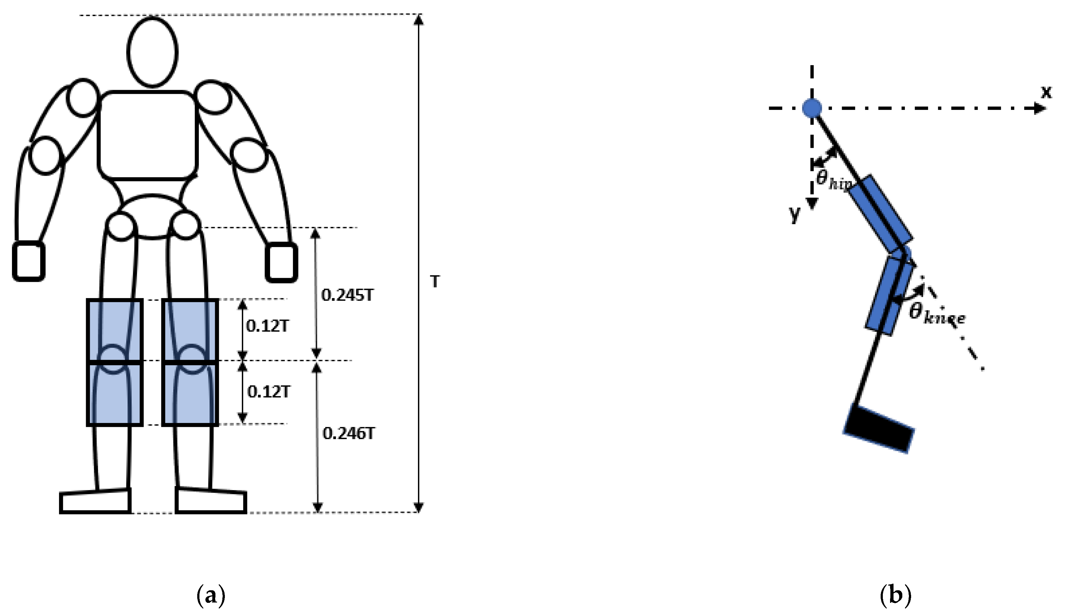
3. Dynamics Analysis
4. Tracking Error
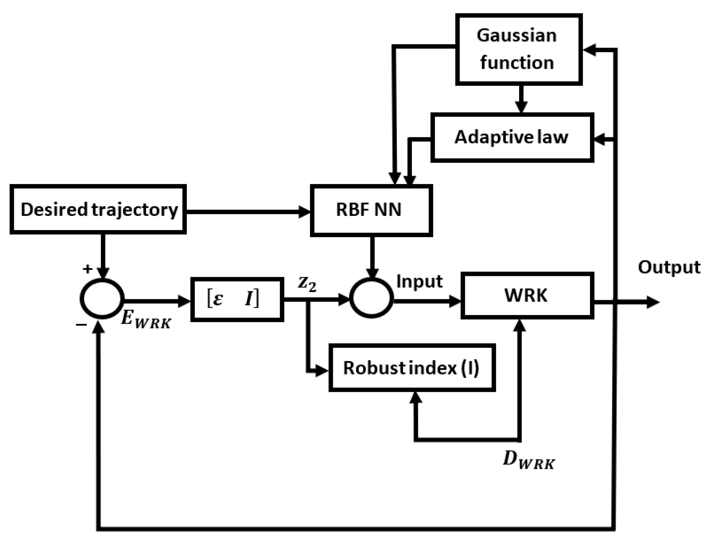
4.1. Control Input
- (1)
- Inputs of vector where is the number of inputs of the RBF NN.
- (2)
- For neural net j in the hidden layer, the Gaussian function value is obtained as:where is the number of neurons in the hidden layer, which is supposed to be equal to the number of the inputs of the RBF NN.
- (3)
- Output, as calculated from the following equation:where and denote the number of outputs and the RBF NN weight, respectively. Hence,
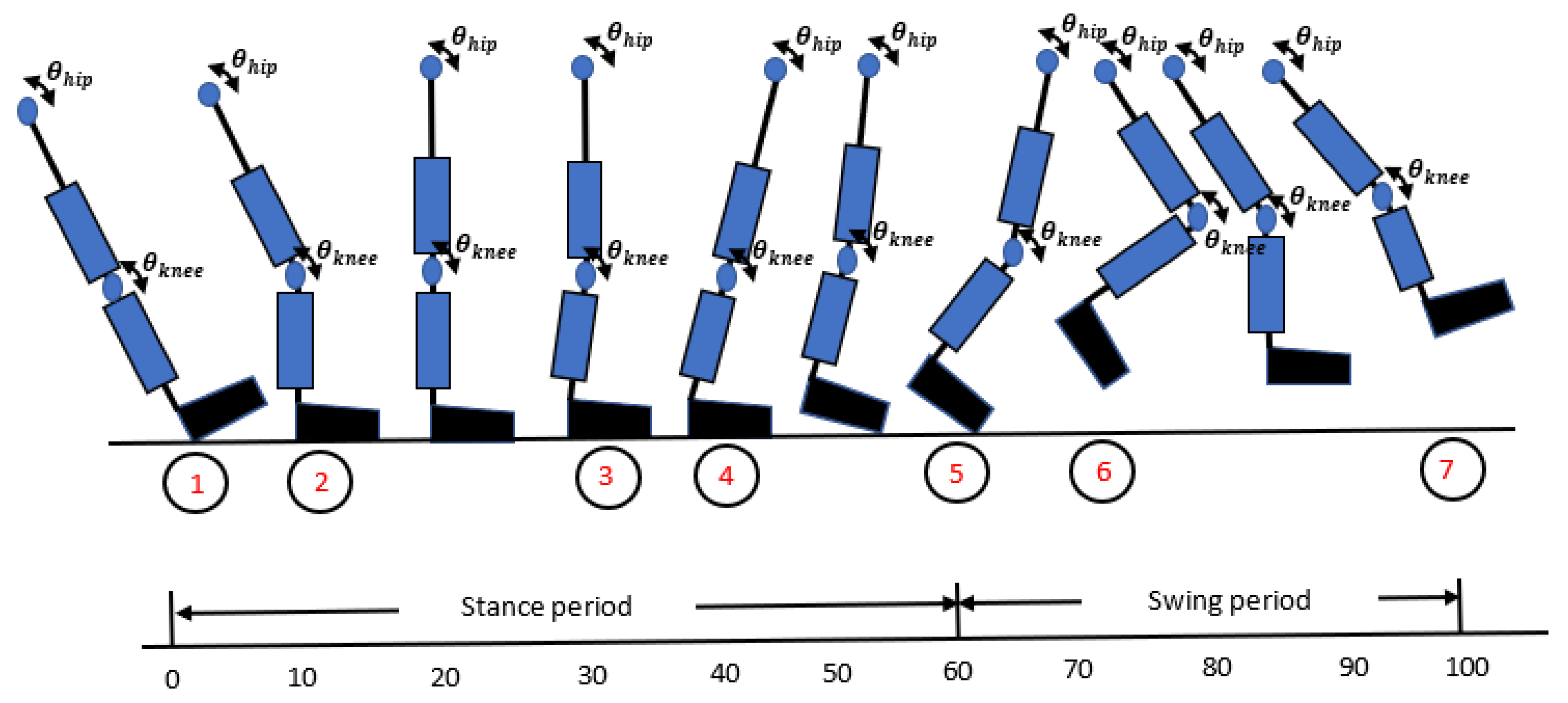
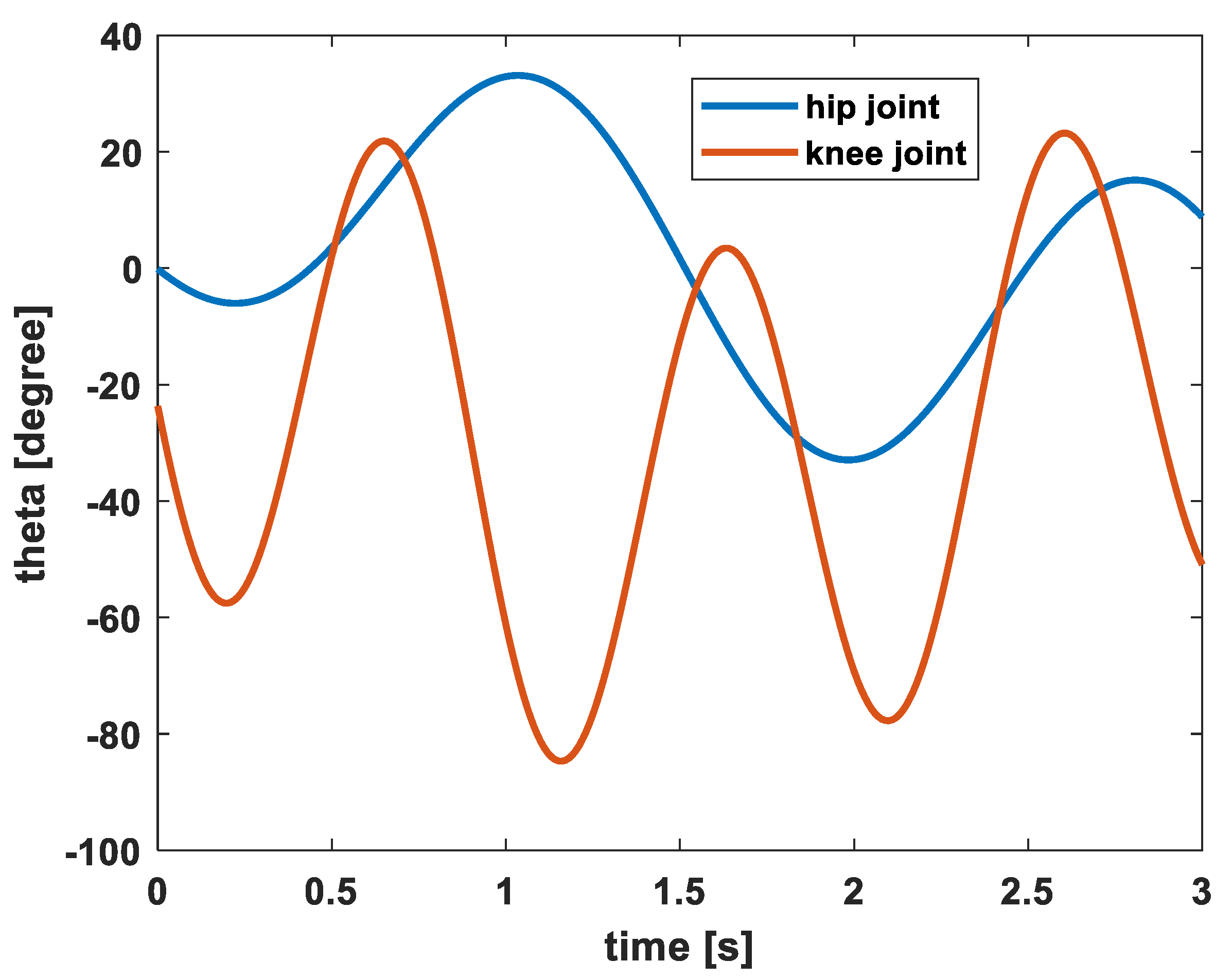
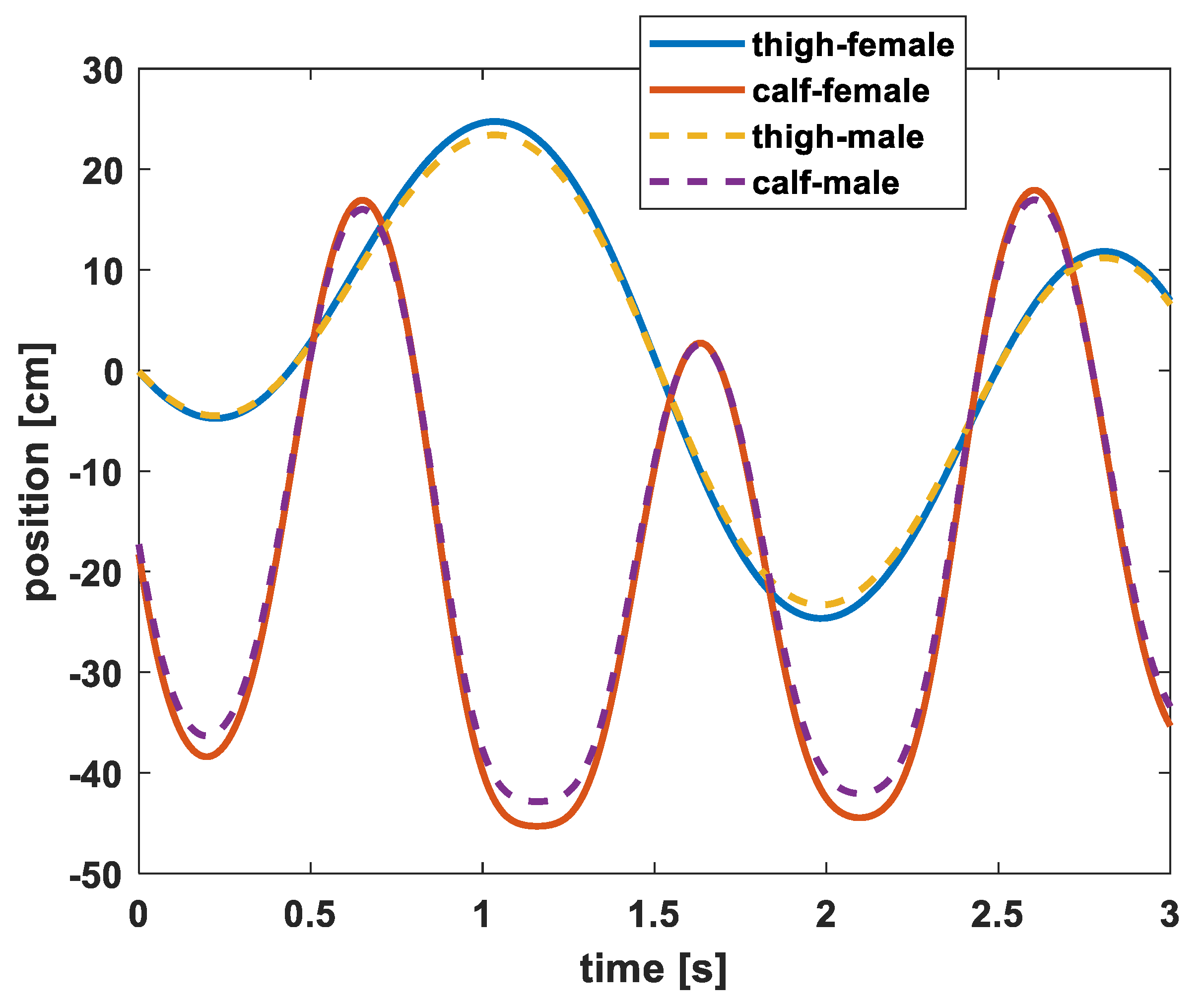
4.2. Hip and Knee Joint Trajectory
- denotes the frequency of motion;
- denotes the amplitude of component of ;
- denotes the amplitude of component of ;
- and denote the harmonic numbers for and , respectively;
- and denote the phase shift for and , respectively.
5. Separation System and Gain
6. RBF NN–Based Adaptive Robust Controller
- The first three components involve the following:
- Regarding the second two components, since and using the adaptive law, i.e., ”, introduced in Equation (46), we obtainHence,
- For the last two components, considering the approximation error as the disturbance and defining , we obtain:
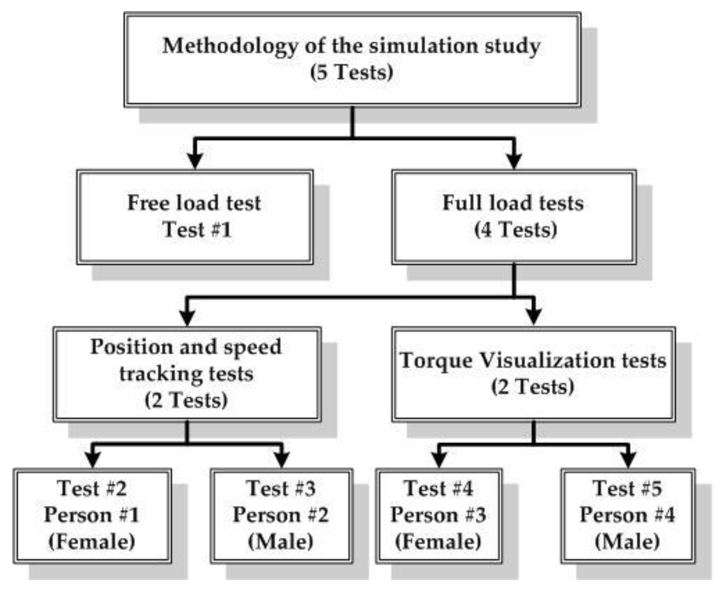
7. Numerical Simulation Validation
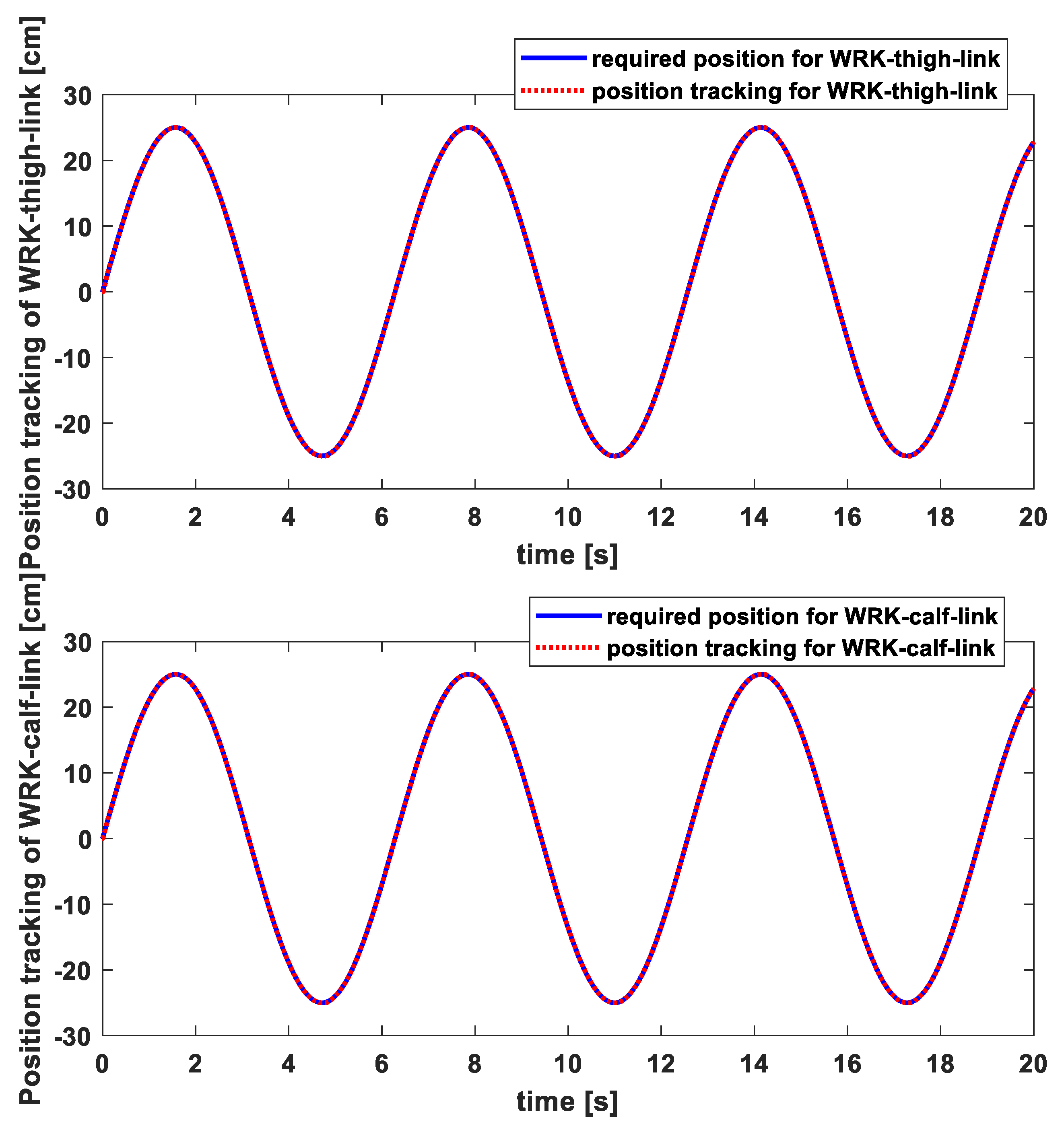
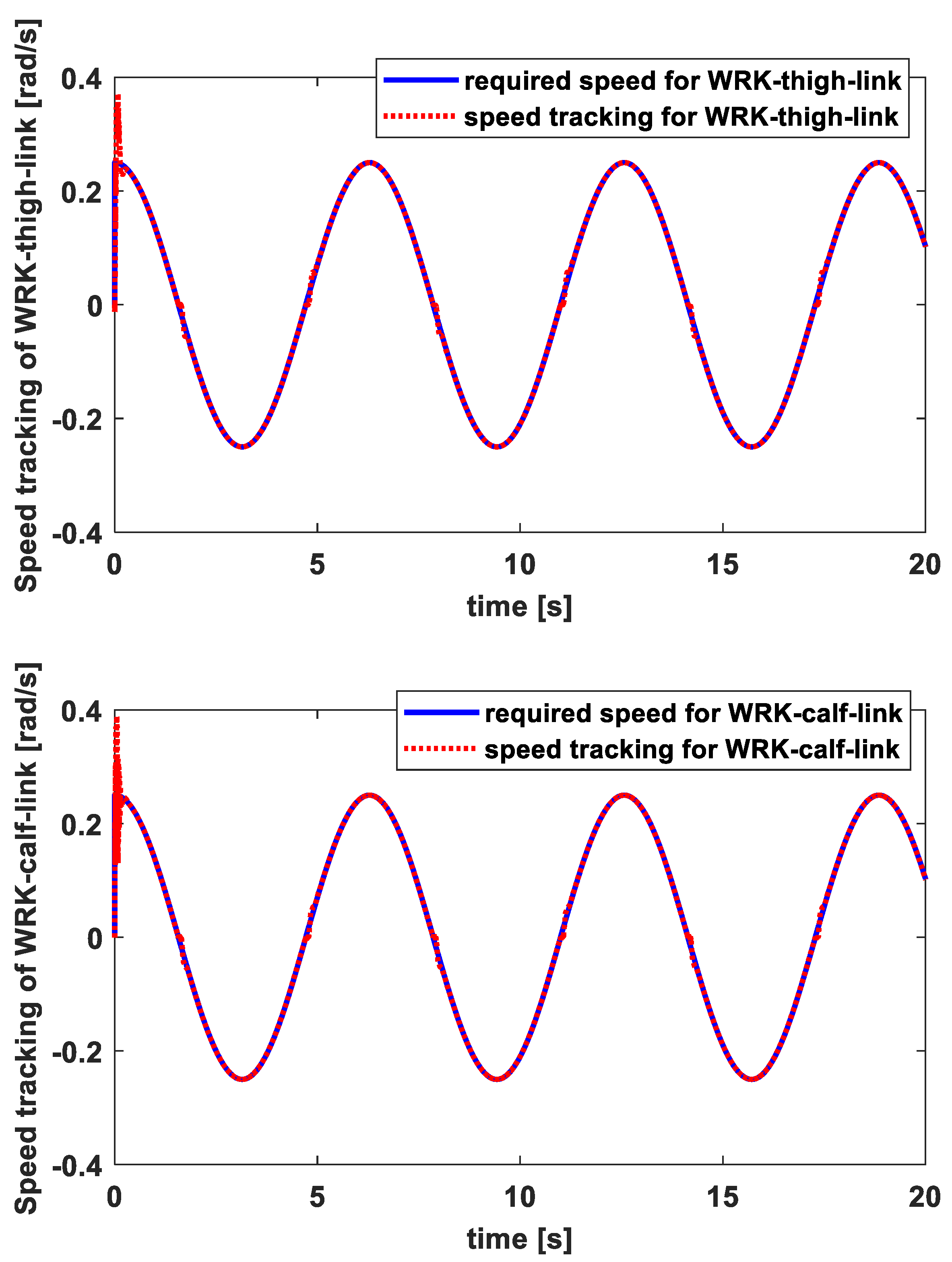
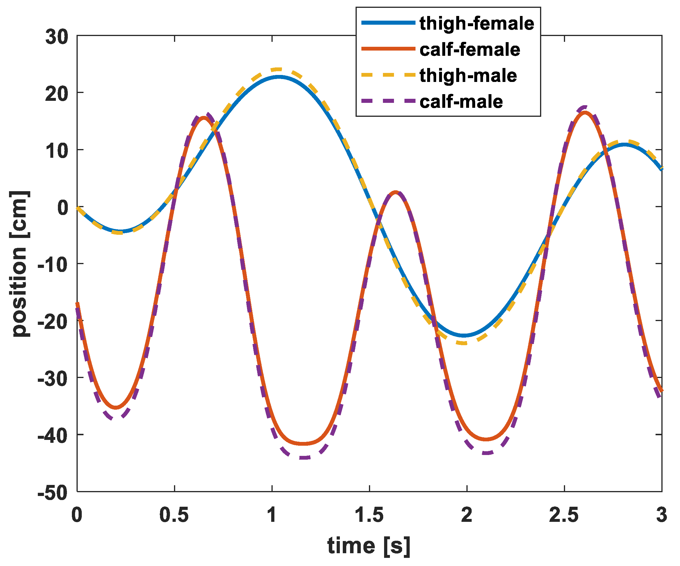
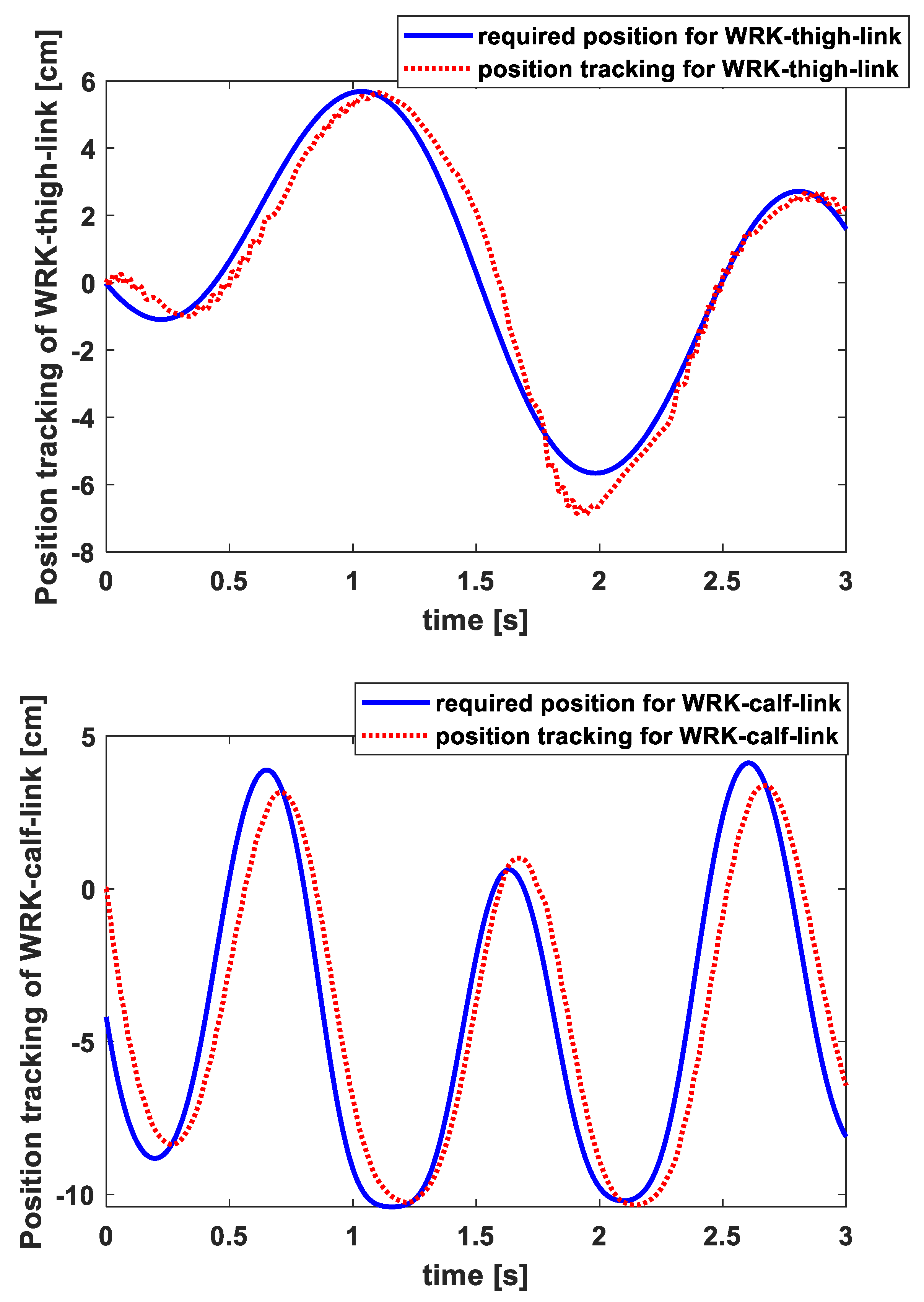
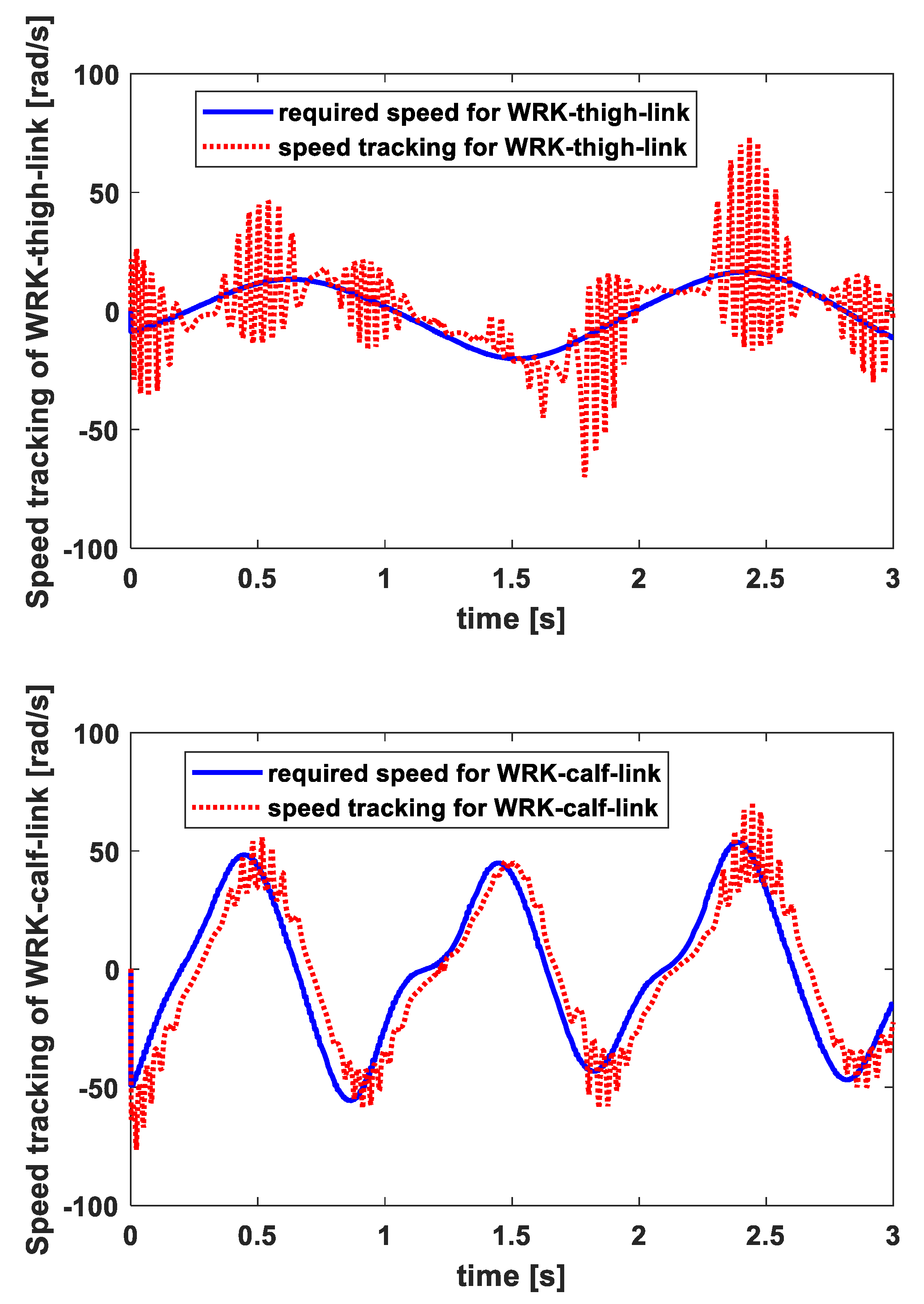
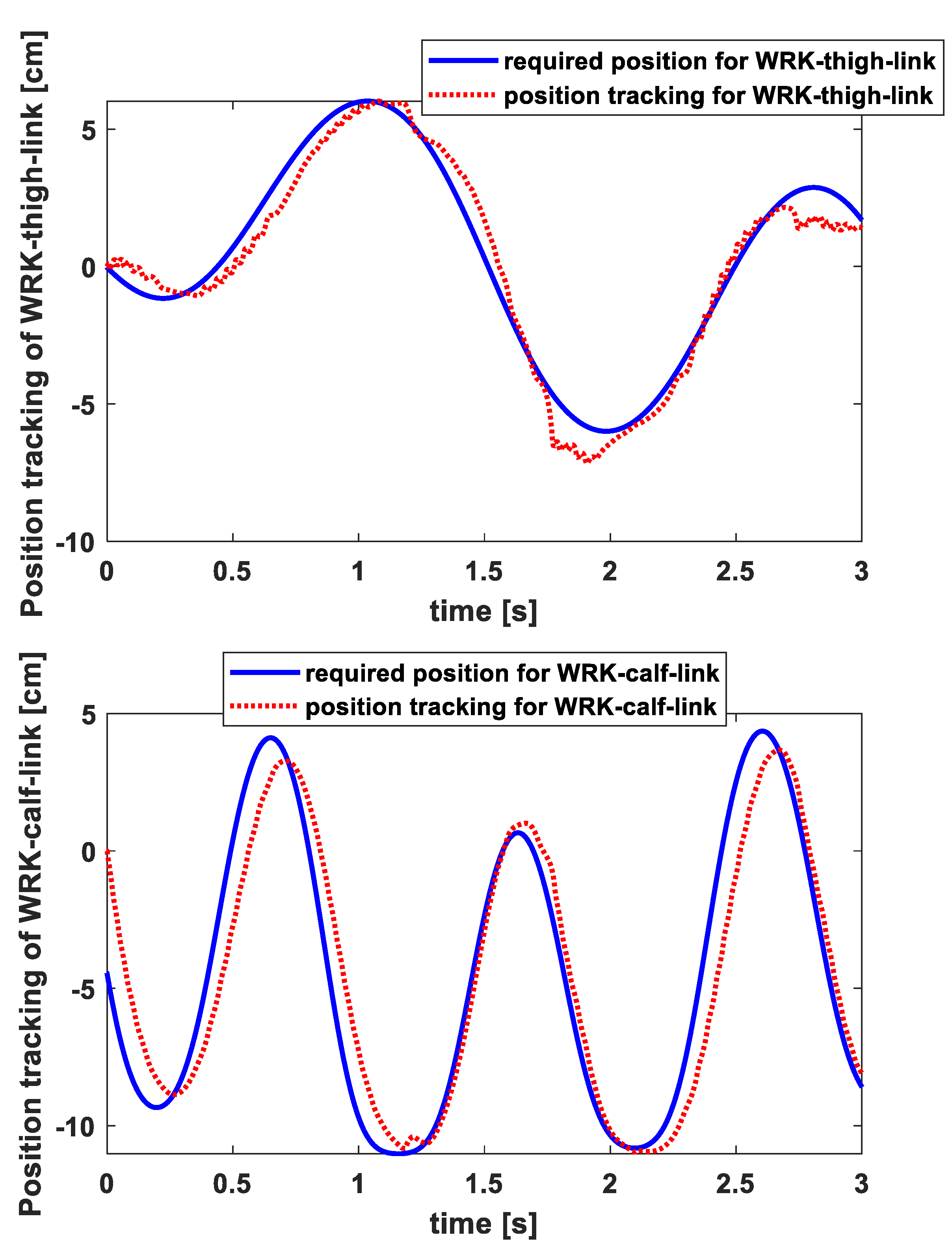
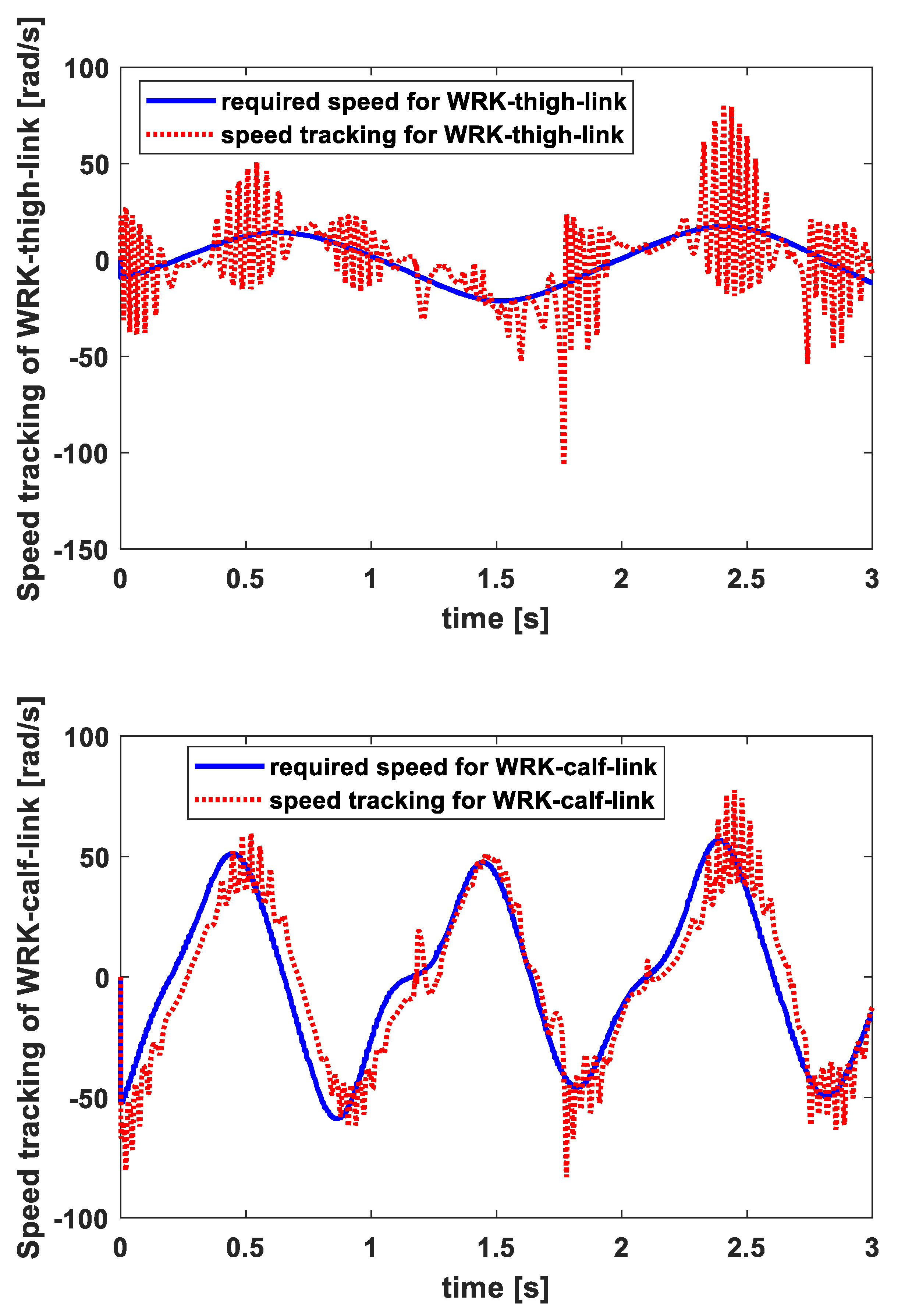
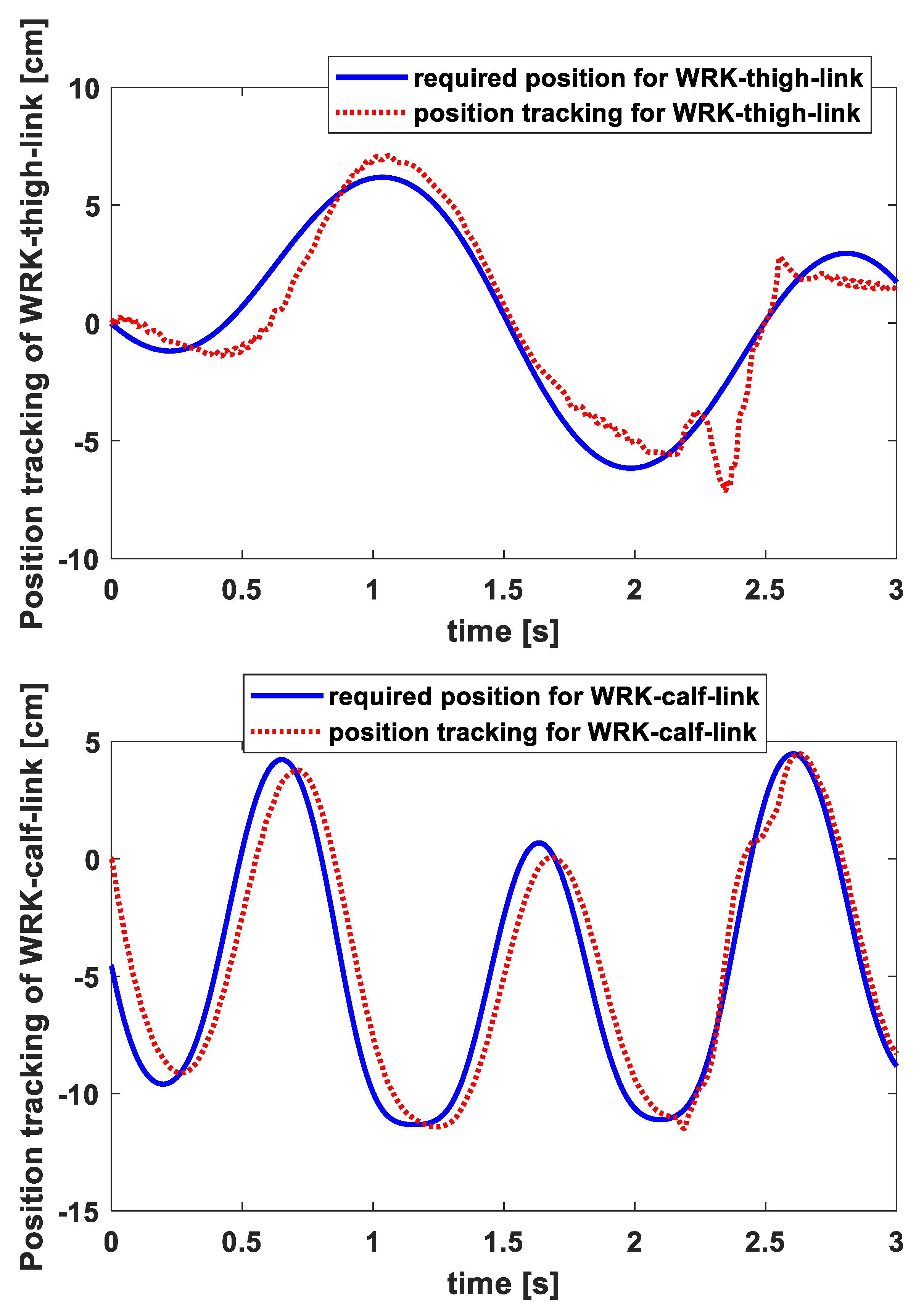
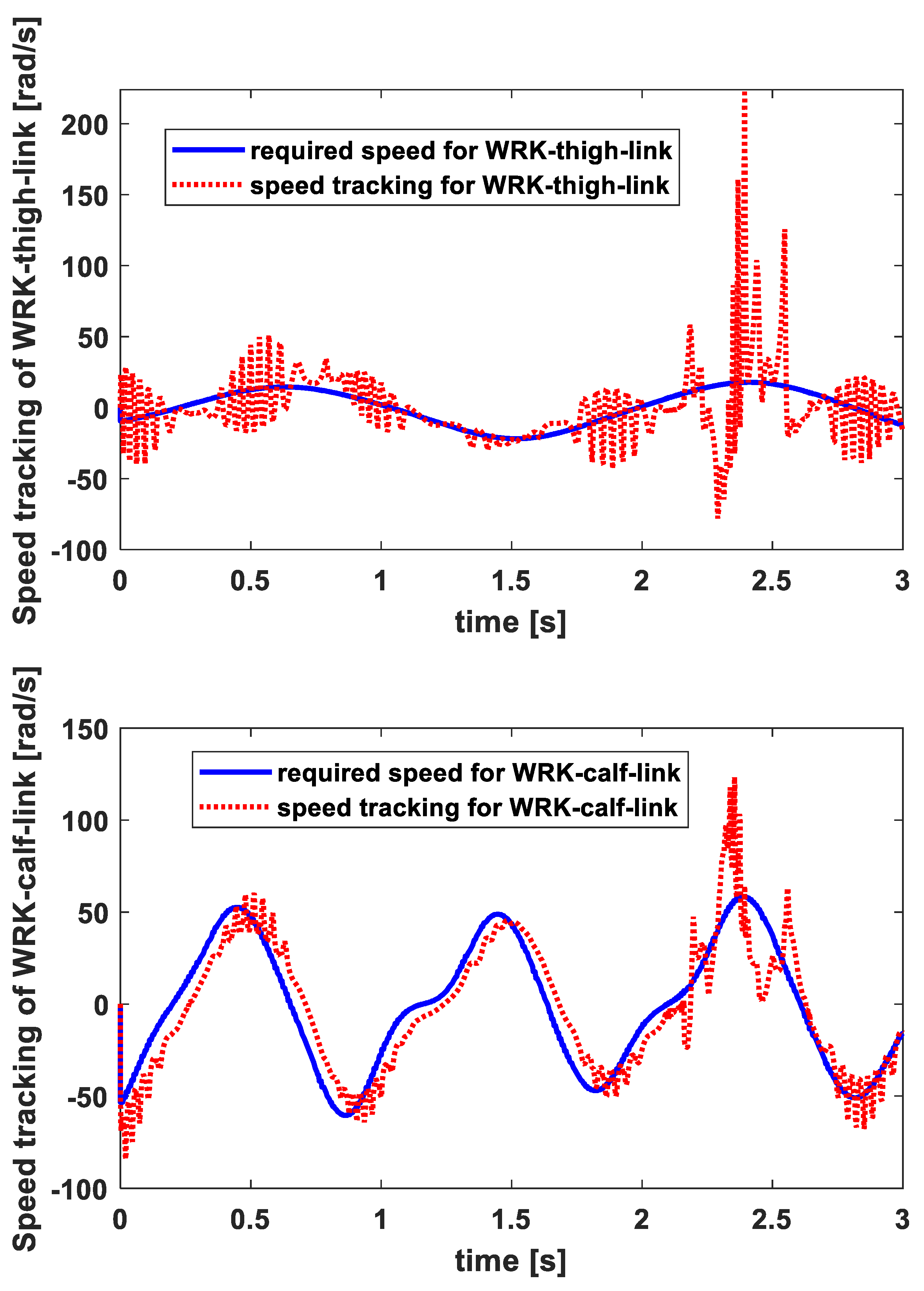
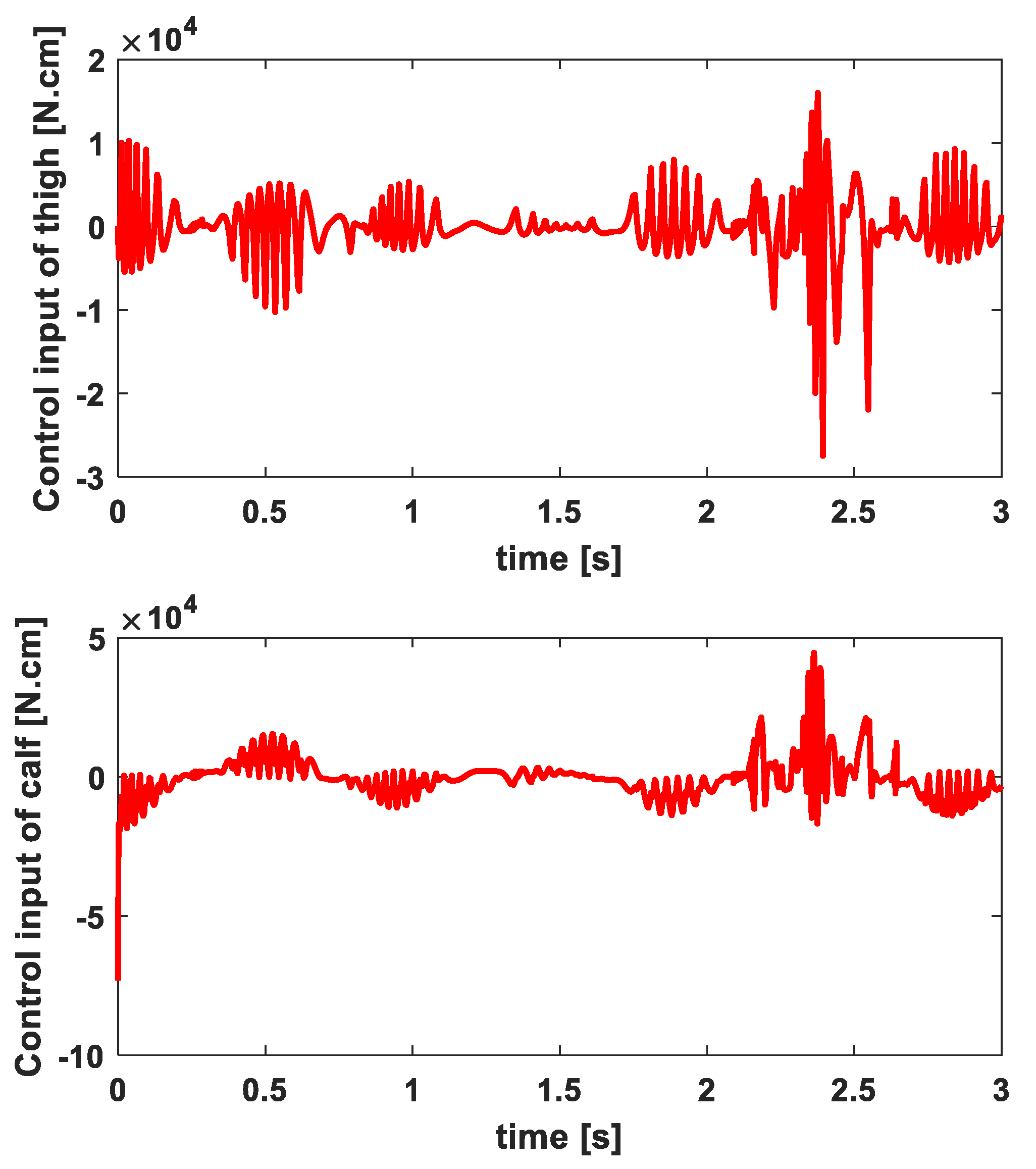
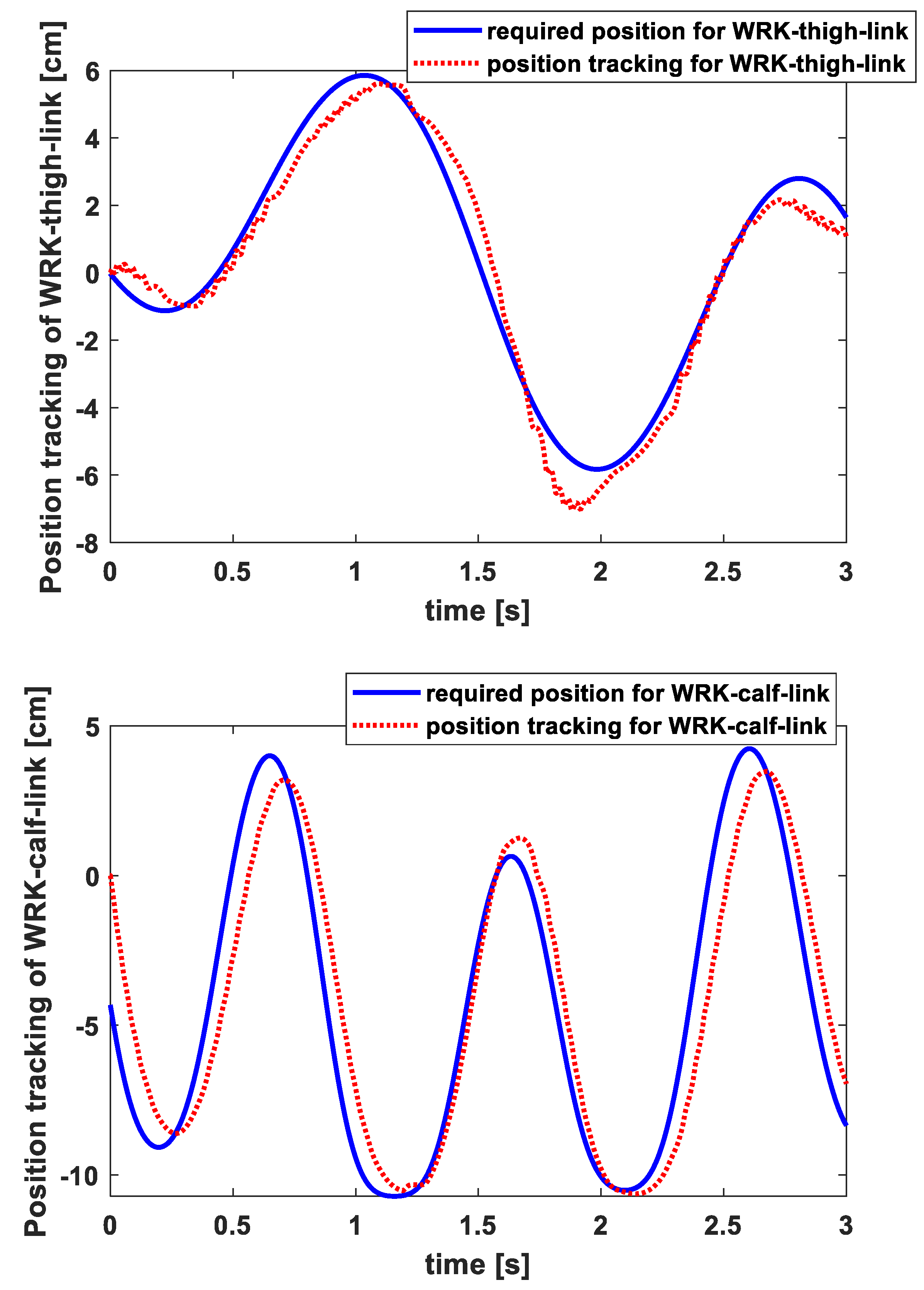
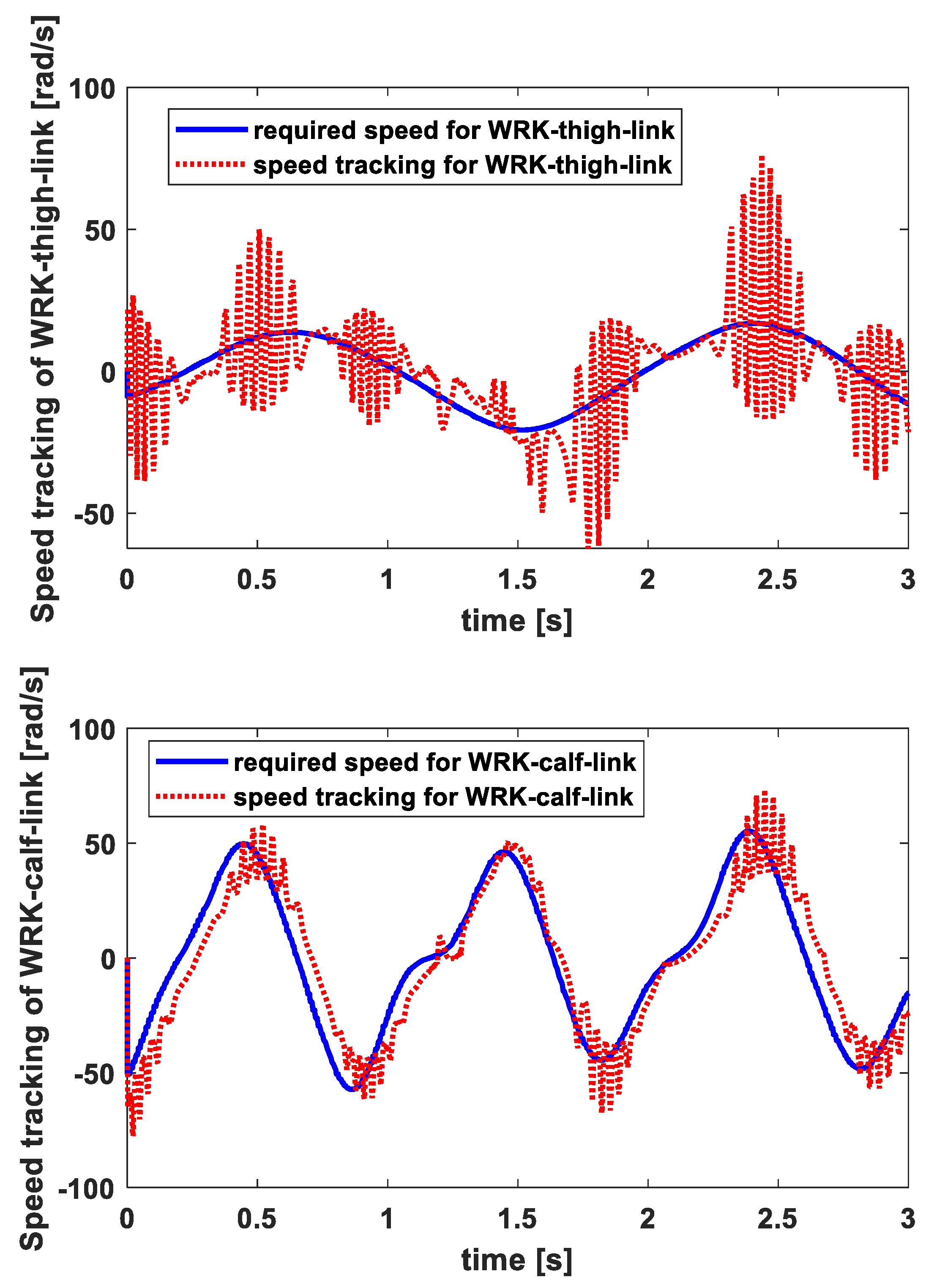
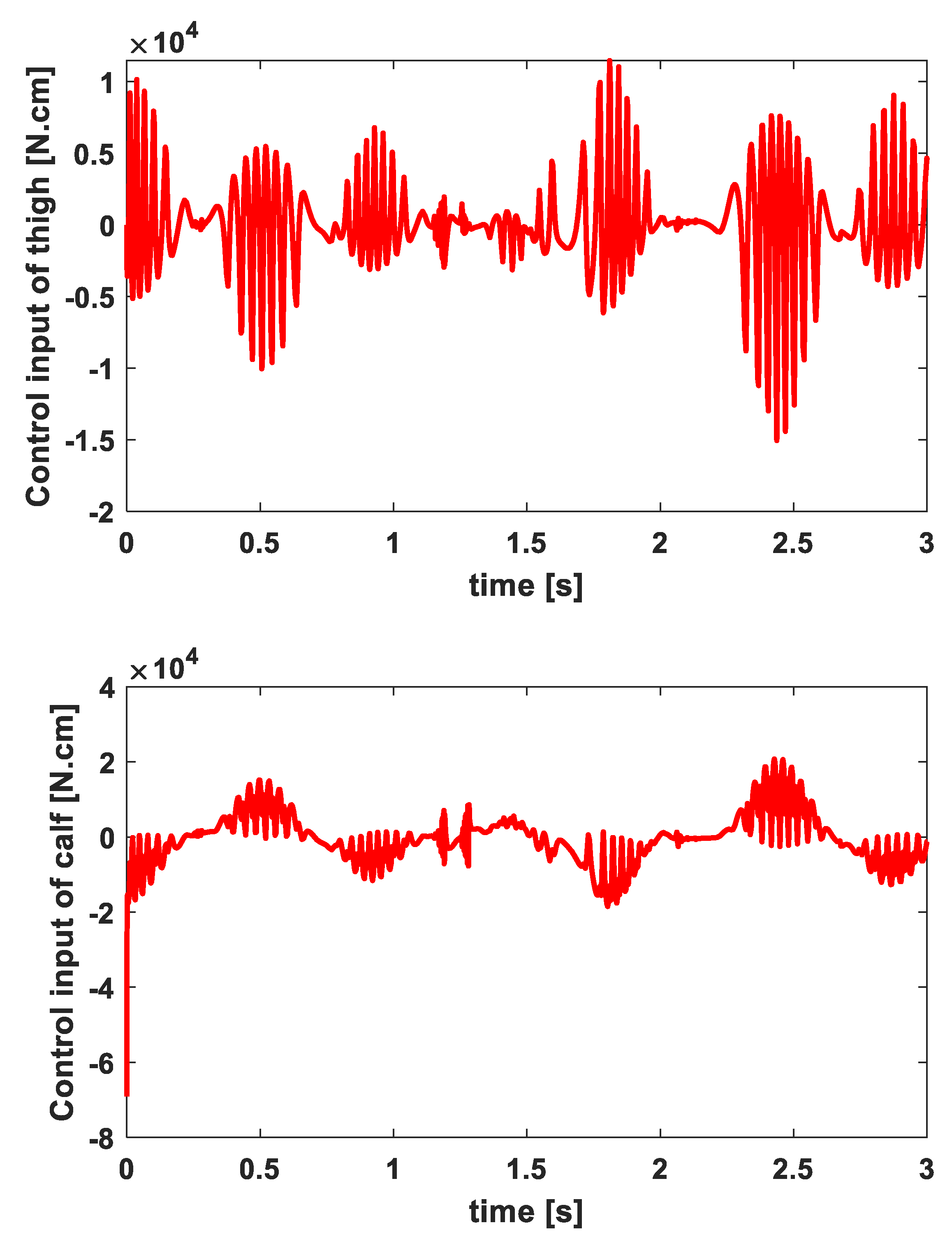
7.1. Simulation Results
7.2. Discussion
8. Conclusions
Author Contributions
Funding
Data Availability Statement
Conflicts of Interest
References
- Hsu, W.-L.; Chen, C.-Y.; Tsauo, J.-Y.; Yang, R.-S. Balance control in elderly people with osteoporosis. J. Formos. Med. Assoc. 2014, 113, 334–339. [Google Scholar] [CrossRef]
- Hassan, M.; Kadone, H.; Ueno, T.; Suzuki, K.; Sankai, Y. Feasibility study of wearable robot control based on upper and lower limbs synergies. In Proceedings of the 2015 International Symposium on Micro-NanoMechatronics and Human Science (MHS), Nagoya, Japan, 23–25 November 2015; pp. 1–6. [Google Scholar] [CrossRef]
- Mohammed, S.; Amirat, Y. Towards intelligent lower limb wearable robots: Challenges and perspectives-State of the art. In Proceedings of the 2008 IEEE International Conference on Robotics and Biomimetics, Bangkok, Thailand, 22–25 February 2009; pp. 312–317. [Google Scholar] [CrossRef]
- Accoto, D.; Sergi, F.; Tagliamonte, N.L.; Carpino, G.; Sudano, A.; Guglielmelli, E. Robomorphism: A Nonanthropomorphic Wearable Robot. IEEE Robot. Autom. Mag. 2014, 4, 45–55. [Google Scholar] [CrossRef]
- Bacek, T.; Moltedo, M.; Langlois, K.; Prieto, G.A.; Sanchez-Villamanan, M.C.; Gonzalez-Vargas, J.; Vanderborght, B.; Lefeber, D.; Moreno, J.C. BioMot exoskeleton-Towards a smart wearable robot for symbiotic human-robot interaction. In Proceedings of the 2017 International Conference on Rehabilitation Robotics (ICORR), London, UK, 17–20 July 2017; pp. 1666–1671. [Google Scholar] [CrossRef]
- Al-Darraji, I.; Kılıç, A.; Kapucu, S. Mechatronic design and genetic-algorithm-based MIMO fuzzy control of adjustable-stiffness tendon-driven robot finger. Mech. Sci. 2018, 9, 277–296. [Google Scholar] [CrossRef]
- Al-Darraji, I.; Kılıç, A.; Kapucu, S. Optimal control of compliant planar robot for safe impact using steepest descent technique. In Proceedings of the International Conference on Information and Communication Technology (ICICT ‘19), London, UK, 25–26 February 2019; Association for Computing Machinery: New York, NY, USA, 2019; pp. 233–238. [Google Scholar] [CrossRef]
- Choo, J.; Park, J.H. Increasing Payload Capacity of Wearable Robots Using Linear Actuators. IEEE/ASME Trans. Mechatron. 2017, 22, 1663–1673. [Google Scholar] [CrossRef]
- Jafri, S.R.A.; Abbasi, M.B.A.; Shah, S.M.U.A.; Hanif, A. BIPATRON (Bionic parageliatron): A wearable robot for rehabilitation… Lets Walk! In Proceedings of the 2017 First International Conference on Latest trends in Electrical Engineering and Computing Technologies (INTELLECT), Karachi, Pakistan, 15–16 November 2017; pp. 1–7. [Google Scholar] [CrossRef]
- Nascimento, L.B.P.D.; Eugenio, K.J.S.; Fernandes, D.H.D.S.; Alsina, P.J.; Araujo, M.V.; Pereira, D.D.S.; Sanca, A.S.; Silva, M.R. Safe Path Planning Based on Probabilistic Foam for a Lower Limb Active Orthosis to Overcoming an Obstacle. In Proceedings of the 2018 Latin American Robotic Symposium, 2018 Brazilian Symposium on Robotics (SBR) and 2018 Workshop on Robotics in Education (WRE), Joao Pessoa, Brazil, 6–10 November 2018; pp. 413–419. [Google Scholar] [CrossRef]
- Cha, K.-H.; Kang, S.J.; Choi, Y. Knee-wearable Robot System EMG signals. J. Inst. Control. Robot. Syst. 2009, 15, 286–292. [Google Scholar] [CrossRef] [Green Version]
- Belkhier, Y.; Shaw, R.N.; Bures, M.; Islam, M.R.; Bajaj, M.; Albalawi, F.; Alqurashi, A.; Ghoneim, S.S.M. Robust interconnection and damping assignment energy-based control for a permanent magnet synchronous motor using high order sliding mode approach and nonlinear observer. Energy Rep. 2022, 8, 1731–1740. [Google Scholar] [CrossRef]
- Belkhier, Y.; Achour, A. Passivity-based voltage controller for tidal energy conversion system with permanent magnet synchronous generator. Int. J. Control. Autom. Syst. 2021, 19, 988. [Google Scholar] [CrossRef]
- Park, Y.-L.; Santos, J.; Galloway, K.G.; Goldfield, E.C.; Wood, R.J. A soft wearable robotic device for active knee motions using flat pneumatic artificial muscles. In Proceedings of the 2014 IEEE International Conference on Robotics and Automation (ICRA), Hong Kong, China, 31 May–7 June 2014; pp. 4805–4810. [Google Scholar] [CrossRef]
- Jeong, M.; Woo, H.; Kong, K. A Study on Weight Support and Balance Control Method for Assisting Squat Movement with a Wearable Robot, Angel-suit. Int. J. Control. Autom. Syst. 2020, 18, 114–123. [Google Scholar] [CrossRef]
- Yuan, Y.; Li, Z.; Zhao, T.; Gan, D. DMP-Based Motion Generation for a Walking Exoskeleton Robot Using Reinforcement Learning. IEEE Trans. Ind. Electron. 2020, 67, 3830–3839. [Google Scholar] [CrossRef]
- Bian, Y.; Shao, J.; Yang, J.; Liang, A. Jumping motion planning for biped robot based on hip and knee joints coordination control. J. Mech. Sci. Technol. 2021, 35, 1223–1234. [Google Scholar] [CrossRef]
- Kagawa, T.; Takahashi, F.; Uno, Y. On-line learning system for gait assistance with wearable robot. In Proceedings of the 2017 56th Annual Conference of the Society of Instrument and Control Engineers of Japan (SICE), Kanazawa, Japan, 19–22 September 2017; pp. 640–643. [Google Scholar] [CrossRef]
- Li, Z.; Deng, C.; Zhao, K. Human-Cooperative Control of a Wearable Walking Exoskeleton for Enhancing Climbing Stair Activities. IEEE Trans. Ind. Electron. 2020, 67, 3086–3095. [Google Scholar] [CrossRef]
- Richards, J. The Comprehensive Textbook of Clinical Biomechanics; Elsevier: Amsterdam, The Netherlands, 2018; ISBN 9780702064951. [Google Scholar]
- Human Body Part Weights. Available online: https://robslink.com/SAS/democd79/body_part_weights.htm (accessed on 2 February 2023).
- Kirsch, N.A.; Bao, X.; Alibeji, N.A.; Dicianno, B.E.; Sharma, N. Model-Based Dynamic Control Allocation in a Hybrid Neuroprosthesis. IEEE Trans. Neural Syst. Rehabil. Eng. 2018, 26, 224–232. [Google Scholar] [CrossRef]
- Han, H.-G.; Qiao, J.-F. Adaptive Computation Algorithm for RBF Neural Network. IEEE Trans. Neural Netw. Learn. Syst. 2012, 23, 342–347. [Google Scholar] [CrossRef]
- Bazargan-Lari, Y.; Eghtesad, M.; Khoogar, A.; Mohammad-Zadeh, A. Tracking Control of A Human Swing Leg Considering Self-Impact Joint Constraint by Feedback Linearization Method. Control. Eng. Appl. Inform. 2015, 17, 99–110. [Google Scholar]
- Zuo, Q.; Zhao, J.; Mei, X.; Yi, F.; Hu, G. Design and Trajectory Tracking Control of a Magnetorheological Prosthetic Knee Joint. Appl. Sci. 2021, 11, 8305. [Google Scholar] [CrossRef]
- Zhang, X.; Lu, Z.; Yuan, X.; Wang, Y.; Shen, X. L2-Gain Adaptive Robust Control for Hybrid Energy Storage System in Electric Vehicles. IEEE Trans. Power Electron. 2021, 36, 7319–7332. [Google Scholar] [CrossRef]
- Coutinho, D.F.; Fu, M.; Trofino, A.; Danes, P. L2 Gain analysis and control of uncertain nonlinear systems with bounded disturbance inputs. Int. J. Robust Nonlinear Control. IFAC Affil. J. 2008, 18, 88–110. [Google Scholar] [CrossRef]
- van der Schaft, A. L2-Gain Analysis of Nonlinear Systems and Nonlinear State Feedback H∞ Control. IEEE Trans. Autom. Control. 1992, 37, 770–784. [Google Scholar] [CrossRef] [Green Version]
- Hendzel, Z. Hamilton–Jacobi inequality robust neural network control of a mobile wheeled robot. Math. Mech. Solids 2019, 3, 723–737. [Google Scholar] [CrossRef]
- Wang, Y.; Sun, W.; Xiang, Y.; Miao, S. Neural Network-Based Robust Tracking Control for Robots. Intell. Autom. Soft Comput. 2009, 2, 211–222. [Google Scholar] [CrossRef]
- Song, Q.; Li, S.; Bai, Q.; Yang, J.; Zhang, A.; Zhang, X.; Zhe, L. Trajectory Planning of Robot Manipulator Based on RBF Neural Network. Entropy 2021, 23, 1207. [Google Scholar] [CrossRef]
- Al-Darraji, I.; Piromalis, D.; Kakei, A.; Khan, F.; Stojmenovic, M.; Tsaramirsis, G.; Papageorgas, P. Adaptive Robust Controller Design-Based RBF Neural Network for Aerial Robot Arm Model. Electronics 2021, 10, 831. [Google Scholar] [CrossRef]
- Liu, J. Radial Basis Function (RBF) Neural Network Control for Mechanical Systems; Springer: Berlin/Heidelberg, Germany, 2013; ISBN 978-3-642-34816-7. [Google Scholar]
- Yang, J.; Na, J.; Gao, G.; Zhang, C. Adaptive Neural Tracking Control of Robotic Manipulators with Guaranteed NN Weight Convergence. Complexity 2018, 2018, 7131562. [Google Scholar] [CrossRef]
- Chaouch, H.; Charfeddine, S.; Ben Aoun, S.; Jerbi, H.; Leiva, V. Multiscale Monitoring Using Machine Learning Methods: New Methodology and an Industrial Application to a Photovoltaic System. Mathematics 2022, 10, 890. [Google Scholar] [CrossRef]
- Charfeddine, M.; Jouili, K.; Jerbi, H.; Braiek, N.B. Linearizing control with a robust relative degree based on a Lyapunov function: Case of the ball and beam system. Int. Rev. Model. Simul. 2010, 3, 219–226. [Google Scholar]
- Qiu, S.; Pei, Z.; Wang, C.; Tang, Z. Systematic Review on Wearable Lower Extremity Robotic Exoskeletons for Assisted Locomotion. J. Bionic. Eng. 2023, 20, 436–469. [Google Scholar] [CrossRef]


| Notation | |
|---|---|
| Height of the person | |
| Weight of the person | |
| Kinetic energy of the WRK system | |
| Kinetic energy of the thigh | |
| Kinetic energy of the calf | |
| Potential energy of the WRK system | |
| Potential energy of the thigh | |
| Potential energy of the calf | |
| Length of the thigh | |
| Length of the calf | |
| Position of the center of thigh in x-axis | |
| Position of the center of thigh in y-axis | |
| Velocity of the thigh | |
| Position of the center of calf in x-axis | |
| Position of the center of calf in y-axis | |
| Velocity of the calf | |
| Angle of the hip | |
| Angle of the knee | |
| Input torque at hip joint | |
| Input torque at knee joint | |
| Mass of the thigh | |
| Mass of WRK device upper arm | |
| Moment of inertia of thigh | |
| Moment of inertia of WRK device upper arm | |
| Mass of the calf | |
| Mass of WRK device lower arm | |
| Moment of inertia of calf | |
| Moment of inertia of WRK device lower arm | |
| Matrix of WRK system inertia | |
| Matrix of Coriolis centrifugal forces | |
| Matrix of gravity | |
| Model errors | |
| External disturbances | |
| Uncertainties | |
| Control input | |
| Inputs of RBF NN vector | |
| Gaussian function | |
| Gaussian function vector | |
| RBF NN weight matrix | |
| Derivative of the estimated RBF NN weight matrix | |
| Error vector | |
| Function of positive value | |
| Input energy | |
| Constant of positive value |
| Benchmark Paper | Compatibility of All WRK Mechanisms | Uncertainties | Disturbances | Adaptivity | Learning Ability | Independence of Knee Joint, Hip Joint | Walking Motion | Self-Working Ability | Safety |
|---|---|---|---|---|---|---|---|---|---|
| Park Y.-L. et al. (2014) [14] | No | Yes | No | No | Yes | No | Yes | Yes | No |
| Eong M. et al. (2020) [15] | Yes | Yes | No | No | No | No | No | Yes | No |
| Yuan Y. et al. (2020) [16] | Yes | No | No | No | Yes | Yes | Yes | No | No |
| Bian Y. et al. (2021) [17] | Yes | No | No | Yes | No | Yes | Yes | Yes | No |
| Kagawa T. et al. (2017) [18] | Yes | No | Yes | No | No | Yes | Yes | Yes | Yes |
| Li Z. et al. (2020) [19] | Yes | No | No | No | No | Yes | Yes | Yes | Yes |
| Current work | Yes | Yes | Yes | Yes | Yes | Yes | Yes | Yes | Yes |
| 1 | 9.17 | 23.9 | 0.6 | 2.8 | 0.5 | −2.3 |
| 2 | 9.5 | 14.2 | 0.04 | 12.5 | 1.5 | 2.5 |
| 3 | 23.5 | 37.1 | 3.7 | 5.18 | 2.4 | 1.2 |
| 4 | 10.4 | 3.6 | 9.8 | 19.4 | −6.7 | −0.36 |
| 5 | −13.07 | 3.12 | 5.4 | 24.8 | 0.2 | −2.36 |
| 6 | 1.8 | 1.9 | 19.1 | 27.3 | −6.4 | −0.36 |
| Person # | Test # | Thigh | Calf | Link-1 | Link-2 |
|---|---|---|---|---|---|
| Person 1 Gender: female Hight = 170 cm Weight = 74 kg | Test 2 | ||||
| Person 2 Gender: Male Hight = 180 cm Weight = 88 kg | Test 3 | ||||
| Person 3 Gender: female Hight = 185 cm Weight = 80 kg | Test 4 | ||||
| Person 4 Gender: Male Hight = 175 cm Weight = 72 kg | Test 5 | ||||
Disclaimer/Publisher’s Note: The statements, opinions and data contained in all publications are solely those of the individual author(s) and contributor(s) and not of MDPI and/or the editor(s). MDPI and/or the editor(s) disclaim responsibility for any injury to people or property resulting from any ideas, methods, instructions or products referred to in the content. |
© 2023 by the authors. Licensee MDPI, Basel, Switzerland. This article is an open access article distributed under the terms and conditions of the Creative Commons Attribution (CC BY) license (https://creativecommons.org/licenses/by/4.0/).
Share and Cite
Jerbi, H.; Al-Darraji, I.; Tsaramirsis, G.; Ladhar, L.; Omri, M. Hamilton–Jacobi Inequality Adaptive Robust Learning Tracking Controller of Wearable Robotic Knee System. Mathematics 2023, 11, 1351. https://doi.org/10.3390/math11061351
Jerbi H, Al-Darraji I, Tsaramirsis G, Ladhar L, Omri M. Hamilton–Jacobi Inequality Adaptive Robust Learning Tracking Controller of Wearable Robotic Knee System. Mathematics. 2023; 11(6):1351. https://doi.org/10.3390/math11061351
Chicago/Turabian StyleJerbi, Houssem, Izzat Al-Darraji, Georgios Tsaramirsis, Lotfi Ladhar, and Mohamed Omri. 2023. "Hamilton–Jacobi Inequality Adaptive Robust Learning Tracking Controller of Wearable Robotic Knee System" Mathematics 11, no. 6: 1351. https://doi.org/10.3390/math11061351