Article

Remote Sensing Imagery Object Detection Model Compression via Tucker Decomposition

1
School of Computer Science, National Engineering Laboratory for Integrated Aero-Space-Ground-Ocean Big Data Application Technology, Shaanxi Provincial Key Laboratory of Speech & Image Information Processing, Northwestern Polytechnical University, Xi’an 710129, China
2
Key Laboratory of Science and Technology on Space Microwave, CAST Xi’an, Xi’an 710100, China
*
Author to whom correspondence should be addressed.
Mathematics 2023, 11(4), 856; https://doi.org/10.3390/math11040856
Submission received: 5 January 2023 / Revised: 4 February 2023 / Accepted: 5 February 2023 / Published: 7 February 2023

Abstract

:
Although convolutional neural networks (CNNs) have made significant progress, their deployment onboard is still challenging because of their complexity and high processing cost. Tensors provide a natural and compact representation of CNN weights via suitable low-rank approximations. A novel decomposed module called DecomResnet based on Tucker decomposition was proposed to deploy a CNN object detection model on a satellite. We proposed a remote sensing image object detection model compression framework based on low-rank decomposition which consisted of four steps, namely (1) model initialization, (2) initial training, (3) decomposition of the trained model and reconstruction of the decomposed model, and (4) fine-tuning. To validate the performance of the decomposed model in our real mission, we constructed a dataset containing only two classes of objects based on the DOTA and HRSC2016. The proposed method was comprehensively evaluated on the NWPU VHR-10 dataset and the CAST-RS2 dataset created in this work. The experimental results demonstrated that the proposed method, which was based on Resnet-50, could achieve up to 4.44 times the compression ratio and 5.71 times the speedup ratio with merely a 1.9% decrease in the mAP (mean average precision) of the CAST-RS2 dataset and a 5.3% decrease the mAP of the NWPU VHR-10 dataset.

1. Introduction

Artificial intelligence, especially deep learning, has delivered significant improvements in several fields, including computer vision, natural language processing, communication signal processing, and automatic driving. Compared with traditional techniques, deep learning has proven to have significant advantages in mid-level and high-level feature extraction. It has been applied to many tasks, including object detection [1] and recognition, object tracking [2], and object segmentation [3].
There are several issues with the satellite data transmission system due to the geometric increase in the amount of remote sensing satellite data and the rapid development of remote sensing technologies. Since clouds cover over 70% of the Earth’s surface, they make up many of the images that remote sensing satellites collect. Usually, these cloud images do not contain valid information and are referred to as invalid images. Another instance is the remote sensing images of the sea surface, where there is no object and little practical use. As a result, one of the most prominent problems is that a large portion of the data acquired by remote sensing satellites is invalid [4]. This invalid data transmission places tremendous pressure on the satellite data transmission system. It wastes precious bandwidth resources [5,6,7] and significantly reduces the utilization of satellite payloads. These problems make it challenging to meet the stringent timeliness requirements of demanding missions, such as Earth observation or some military tasks. Notably, the current problems faced by remote satellites can be solved with onboard image processes, which can recognize the invalid data and discard this invalid data onboard directly.
Object detection is one of the essential tasks of remote sensing image processing [8]. It is also the basis for advanced applications, such as remote sensing image analyses, image understanding, and scene understanding. In addition, onboard object detection can improve satellite data relay services in terms of the amount of user data and timeliness. Therefore, it has attracted the increasing attention of many scholars.
There are two typical scenarios for remote sensing object detection. One is to transmit remote sensing images to the ground via a satellite data transmission system, and then object detection is performed [9]. In this scenario, the object detector is deployed on the ground without consideration of storage, the computational cost, or the power consumption limitations imposed by the space environment. Another strategy is to perform object detection directly on satellites [10]. In this situation, it is necessary to deploy the detector on board and to consider all of the resources that the satellite can offer.
Onboard object detection is more attractive for military and civilian missions. First, this approach can respond to changes on the ground in real time and feed back the results, particularly for military tasks or disaster monitoring. Second, no actions are required to transmit the original data to the ground station. There is a large amount of redundant data in the images collected by the satellite, and sending all the data back to the ground station would undoubtedly waste valuable satellite bandwidth resources. With object detection on board, only valuable data would be transmitted back to the ground. It would significantly reduce the waste of bandwidth.
Limited by the space environment, the computational and storage capacities onboard are significantly inferior to those on the ground [11,12]. Deep learning algorithms are computationally expensive and memory intensive. The improved performance of these algorithms comes at the expense of high computational and storage resource consumption [13]. Deploying deep learning algorithms on satellites is more challenging than on the ground, not only in terms of balancing performance and resources but also in terms of the onboard implementation of the algorithms. Therefore, onboard object detection model compression is an urgent request in current research.
Model compression is a practical approach to reducing model complexity which can significantly reduce the number of parameters and the computing costs of the model without significantly degrading the performance. It was used to reduce the CNN model size and hardware requirements of the CNN deployment to solve the problems mentioned above when the object detector was deployed on the satellite in this paper. Among several model compression methods, the low-rank decomposition method is an emerging tool for large-scale data approximation that can be approximately represented in highly compressed formats and that is widely adopted [14,15,16,17].
Decomposed factors are directly mapped to convolution layers without the reconstruction of these factors to high-order tensors. This method is the most popular approach to CNN model compression based on low-rank decomposition. In [14], the four factors of the CP (canonical polyadic) decomposition [15] of the convolution kernel tensor were considered to be one pointwise convolution kernel, two depthwise convolution kernels, and one pointwise convolution kernel, respectively. In [16], the four factors of the Tucker decomposition [17] of the convolution kernel tensor were considered to be a pointwise convolution kernel, a standard three × three convolution kernel, and another pointwise convolution kernel, respectively.
Previous works explored this technology on VGG [18], and AlexNet [19] demonstrated promising results for model decomposition. Still, the situation varies when decomposing Resnet [
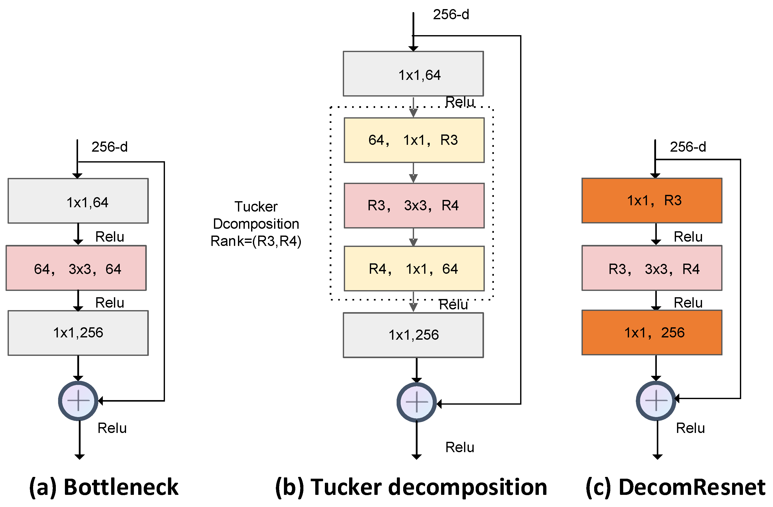
20], which is constructed with the bottleneck shown in Figure 1a. The three × three convolution kernel tensor in the bottleneck can be decomposed into a pointwise convolution kernel, a standard three × three convolution kernel, and another pointwise convolution kernel [16] as shown in Figure 1b. In this case, two pointwise convolutional layers are cascaded together. The number of input channels reduces, but the convolution layers increase. The convolutional layers increase the computation time because the CNN models are computed layer by layer. To solve this problem, we merged the two pointwise convolutional layers and constructed a novel module called DecomResnet as shown in Figure 1c.
The main contributions of this paper are summarized as follows:
(1)
A model compression method was proposed for remote sensing image object detection based on Tucker decomposition which consisted of four steps:
Step 1:
model initialization;
Step 2:
initial training;
Step 3:
trained model decomposition and reconstruction;
Step 4:
fine-tuning.
(2)
The DecomResnet module was proposed based on Tucker decomposition. It was used to construct the backbone of the object detection model. The experimental results showed that the proposed module significantly reduces the number of parameters and computational costs with a slight decrease in performance.
(3)
To verify the performance of the compression model proposed in this paper, the model was validated on the NWPU VHR-10 dataset. The experimental results indicated that the proposed method is an effective approach to model compression.
(4)
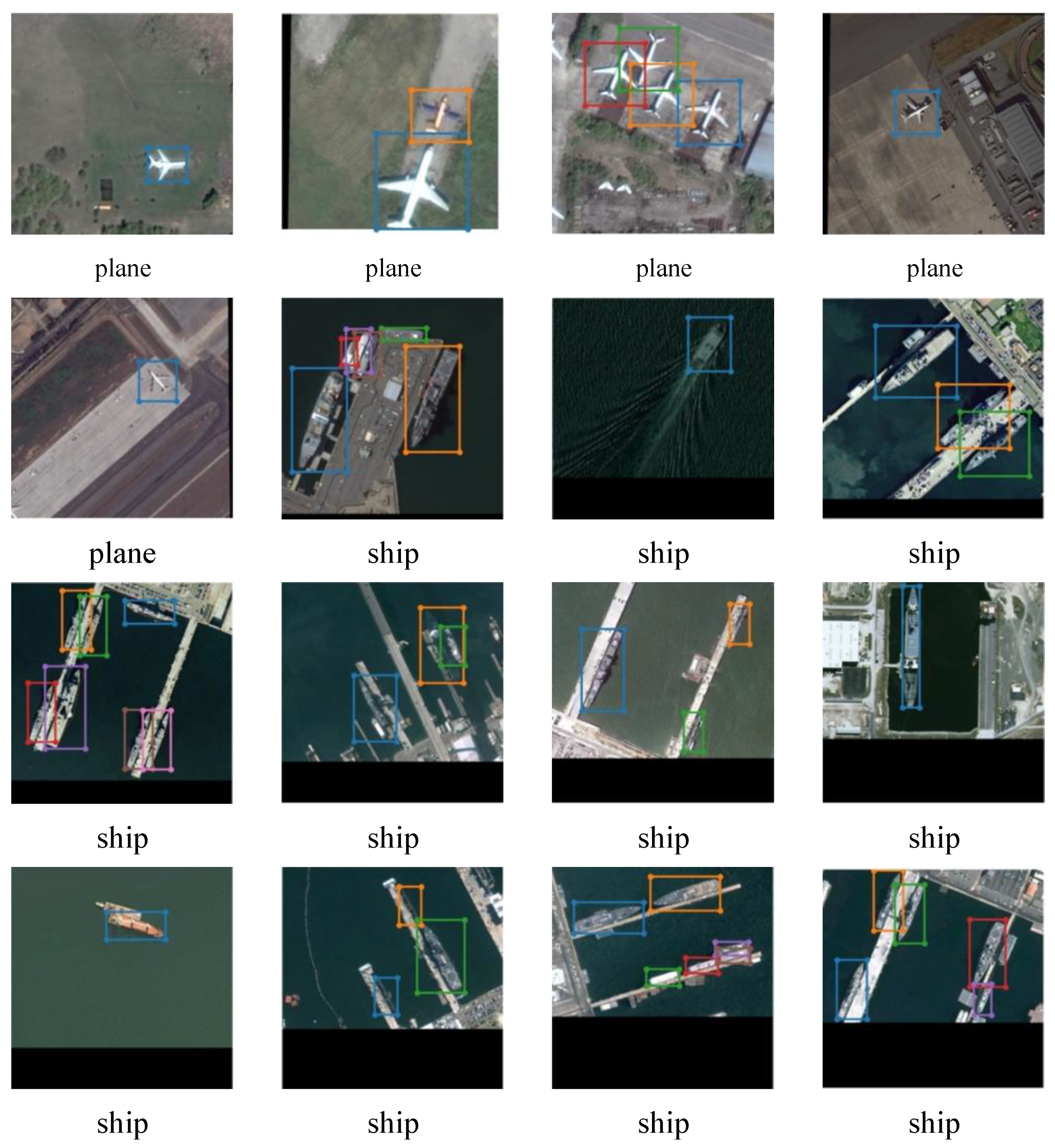
For our practical engineering application requirements, we constructed a remote sensing dataset named CAST-RS2 which contained only two types of objects according to the mission requirements and the characteristics of remote sensing objects. The proposed method was also verified on this dataset.

2. Related Work

Model compression methods can be broadly categorized into knowledge distillation [21], pruning [22], quantization [23], low-rank decomposition [24], and lightweight models [25].
Knowledge distillation is commonly used in migration learning, also known as student–teacher networks. The key concept is to train a deep teacher network and then to teach a small student network that mimics the teacher, which is deployed after training. The teacher model can be a single large model or a collection of individually trained models. The main idea of pruning is to remove the redundant parameters from the large model to obtain a small model.
The main idea of pruning is to grow a large model and then to prune away weights to end up with a much smaller but effective model. Luo et al. [22] reduced Resnet through pruning. The Resnet that was compressed through pruning is similar to DecomResnet. However, they are not the same, which is reflected in the following aspects:
First, the number of channels in the convolutional layers is different. Although both have three layers, the first layer is a one × one convolution, the second layer is a three × three convolution, and the third layer is a one × one convolution, the number of channels in the convolution layers is not the same. A greedy algorithm obtains the channels of the first two convolutional layers in ThiNet. In this paper, however, the rank (R3, R4) acquired by the VBMF method determined how many channels were present in the first two convolutional layers.
Second, the method of reducing the number of channels is different. ThiNet adopts the pruning method, i.e., the unimportant channels in the convolution kernel are removed directly. However, in this paper, the Tucker decomposition factors were used as the convolution kernel to reduce the number of channels.
Third, the compressed objects are inconsistent. ThiNet does not prune the first two layers in the bottleneck. Some of them will not be pruned. However, all the three × three convolutional layers in the bottleneck were decomposed in this paper.
Fourth, the process of model compression is different. ThiNet prunes CNN models layer by layer. Its framework is filter selection, pruning, and fine-tuning. Our decomposed framework was initialization, training, obtaining the ranks, and fine-tuning.
Fifth, the compression ratio is not the same. The compression ratio of ThiNet is set manually. However, the compression ratio of the method proposed in this paper was determined by the ranks of Tucker decomposition.
The main idea of quantization is to store the weights and activation tensors in lower-bit precision representations rather than the 16-bit or 32-bit precision representations.
In recent years, some researchers have been working on designing more compact, less computationally intensive, and more efficient network structures, such as the fire module of SqueezeNet [25], the residual structure of Resnet [20], the inception module of Googlenet [26], etc. These lightweight modules are composed of tiny convolutions, such as one × one convolutions or three × three convolutions, which can effectively reduce the number of model parameters and the volume of operations.
Deep models are usually overparameterized, and the weight matrix components usually reside in low-rank subspaces [27]. Therefore, low-rank decomposition is considered one of the efficient deep compression schemes and is generally used to compress deep models.
The most popular low-rank decomposition techniques are canonical polyadic decomposition (CP) [14], Tucker decomposition [16], and tensor-train decomposition [28,29]. CP decomposition presents an n-way tensor as the sum of r ( r is the minimum rank) rank-1 terms. This method is simple and efficient. However, its drawback is that finding the r rank is an NP-hard problem. Tucker decomposition approximates the original tensor by multiplying a core tensor by a factor matrix along with each pattern. Tensor-train (TT) decomposition expresses the tensor as a string of smaller (three-way) core tensors. It maintains a simplicity similar to CP decomposition and achieves a higher compression rate. Several works [30,31] focus on decomposing the convolutional weight tensors to reduce the parameters more efficiently and to reconstruct the decomposed factors during inference without significant performance loss. The procedure of this approach is as follows: First, these methods train the model for a few epochs, which is called initialized training. Second, the weight tensor obtained from initialized training is decomposed. Finally, the decomposed model is retrained, which is called fine-tuning. In the inference phase, the higher-order convolutional weight tensor is reconstructed by lower-order factors again. The advantage of this approach is that the convolution structure does not change, but the convolutional kernel must be rebuilt.
Another approach is to decompose the weight tensor and to construct a new convolution module based on the decomposed factors [14,16]. In [14], a convolution module was created based on the CP decomposition factor, consisting of a point convolution, a separable convolution, and another point convolution. In [16], a convolution module was constructed based on the Tucker decomposition factor, which consists of a point convolution, a regular convolution, and a point convolution. Essentially, these methods achieve model compression by transforming complex CNN models into lightweight models through low-rank decomposition. In the inference stage, these methods do not require the reconstruction of the low-rank tensor into a high-rank tensor, which is suitable for applications in resource-limited environments. Inspired by these two works, we proposed a CNN model compression method based on Tucker decomposition.
In addition to the most popular methods mentioned above, the hierarchical Tucker (HT) method [32] and the Kronecker product decomposition (KPD) [33] method are also used to compress the weights of the convolution layers.
The hierarchical Tucker (HT) method decomposes the kernel weight tensor into two load matrices and smaller three-way tensors. The load matrices are equal to one × one convolution layers, and the three-way tensors are equal to one-dimensional convolution layers.
The KPD method approximates the original matrix with two smaller Kronecker factor matrices. This method can also be extended to the multidimensional nearest Kronecker product problem [33]. The rank is an essential hyperparameter in the low-rank decomposition process. However, the solution to the optimal rank is an NP-hard problem, which is difficult to obtain. Several rank selection methods have been proposed to obtain the rank of tensors. A fitness-based rank selection method was proposed in [34]. However, this rank selection method has limitations in selecting multiple ranks and has convergence problems in the optimization process. SVD (singular value decomposition) was used to solve for the optimal rank in [35], but this solution method is very time-consuming. A heuristic method was used to select the rank in [16], but the CNN structure determines the desired rank and the dataset used.
Miao et al. [36] recently proposed a budget-aware rank selection method that can calculate tensor ranks via one-shot training. Although it can automatically select the proper tensor ranks for each layer, it may obtain different ranks when the training environment changes, such as the dataset and training hyperparameters.
The variational Bayesian matrix factorization (VBMF) method was proposed in [37]. Although this method generates suboptimal ranks, it is a highly reproducible approach and is currently considered adequate.

3. Proposed Method

3.1. The Baseline Object Detection Model Analysis

In this paper, we took RetinaNet as the baseline because it can offer a better speed/accuracy trade-off and because it is a promising onboard deployment candidate model. We first analyzed the baseline model, focusing on the number of parameters in each part of the baseline, and then decomposed the weight tensors.
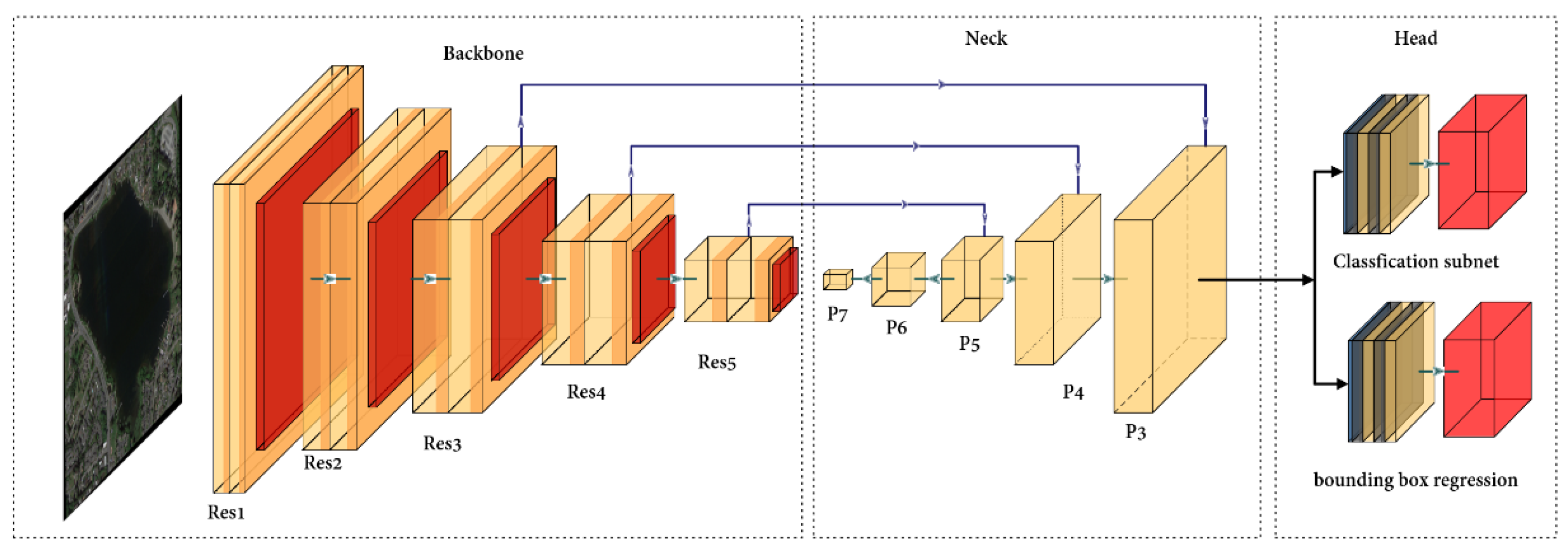
As shown in Figure 2, the object detector consists of three parts: the backbone, neck, and head.
Among these three parts, the backbone has the most parameters, accounting for more than 60% of the detector parameters. Huang et al. [30] pointed out that the backbone has many redundant parameters. Decreasing the number of backbone parameters is an effective way to reduce CNN complexity. The backbone consists of a finite number of convolutional modules. Each convolutional layer of these modules is a 4D tensor.
Due to its excellent feature extraction capability, Resnet is widely used in object detection tasks. The parameters of Resnet mainly consist of one × one convolutional layers and three × three convolutional layers. Taking Resnet-50 as an example, the number of one × one convolution layer parameters and three × three convolution layer parameters account for 47.4% and 44.44% of the backbone, respectively. The number of parameters in three × three convolution layers can be reduced through tensor decomposition, but the number of parameters in one × one convolution layers cannot be reduced similarly. When the input image size is 512 × 512, the FLOPs of the backbone is 21.52 GMac, which accounts for 40.38% of RetinaNet.
The neck of RetinaNet adopts the feature pyramid network (FPN). The advantage of the FPN is that it fuses shallow and deep features. The output features contain deep semantic and shallow spatial information that is beneficial to multiscale object detection. The neck has five different scales of feature maps (P3–P7). P3, P4, and P5 consist of one × one and three × three convolution layers. P6 and P7 consist of three × three convolution layers. The number of parameters in the neck is 8.00 M, accounting for 22.04% of all the detector parameters. The computational cost of the neck is 4.43 GMac, accounting for 8.30% of RetinaNet.
The head of RetinaNet consists of two parts: bounding box regression and object classification. Five feature layers share the head, where the number of classification branch parameters is 2.36 M, accounting for 6.50% of RetinaNet. The computational cost is 12.88 GMac, accounting for 24.17% of RetinaNet. The regression branch is the same as the classification branch. The head is essential for the compression of the detector.
The backbone of RetinaNet; the backbone and detection head of RetinaNet; and the backbone, detection head, and neck of RetinaNet were each decomposed in this work to implement model compression.

3.2. Decomposed Convolutional Model

To reduce the convolutional parameters, we introduced a tensor decomposition method. The parameter size of each layer in the object detection network was D × D × S × T . The numbers of output and input channels were T and S , respectively. The width and height of the convolutional kernel were D . It could be seen that a four-dimensional tensor could represent the convolutional kernel. If the input feature was X , its size would be H W S , and if the output feature was Y , its size would be H × W × T , which could be expressed as Equation (1).
Y h , w , t = i = 1 D j = 1 D s = 1 S K i , j , s , t X h i , w j , s h i = ( h 1 ) Δ + i p and w j = ( w 1 ) Δ + j p
where K is a fourth-order convolution kernel tensor, its size is D × D × S × T , ∆ is the stride, and p is the zero-padding size.
We considered model compression as a tensor decomposition problem. The convolutional neural network was compressed if the total elements of the low-dimensional tensors were less than the total elements of tensor K .
Therefore, Tucker decomposition was used to decompose convolutional kernel tensor K . The decomposition of the convolution kernel could be expressed as Equation (2).
K i , j , s , t = r 1 = 1 R 1 r 2 = 1 R 2 r 3 = 1 R 3 r 4 = 1 R 4 C r 1 , r 2 , r 3 , r 4 K i , r 1 ( 1 ) K j , r 2 ( 2 ) K s , r 3 ( 3 ) K t , r 4 ( 4 )
where R 1 , R 2 , R 3 , and R 4 are the ranks of Tucker decomposition; C R 1 × R 2 × R 3 × R 4 is a smaller four-dimensional tensor; and K ( 1 ) D × R 1 , K ( 2 ) D × R 2 , K ( 3 ) S × R 3 , and K ( 4 ) T × R 4 are two-dimensional matrices. Then we substituted Equation (2) into Equation (1), where the convolution operation could be expressed as Equation (3).
Y h , w , t = i = 1 D j = 1 D s = 1 S ( r 1 = 1 R 1 r 2 = 1 R 2 r 3 = 1 R 3 r 4 = 1 R 4 C r 1 , r 2 , r 3 , r 4 K i , r 1 ( 1 ) K j , r 2 ( 2 ) K s , r 3 ( 3 ) K t , r 4 ( 4 ) ) X h i , w j , s
The literature [16] states that not all modes must be decomposed. Since mode-1 and mode-2 were relatively small, usually three or five, there was no need for further decomposition. At this point, the Tucker decomposition of the convolution kernel could be expressed as Equation (4).
K i , j , s , t = r 1 = 1 R 1 r 2 = 1 R 2 r 3 = 1 R 3 r 4 = 1 R 4 C i , j , r 3 , r 4 K s , r 3 ( 3 ) K t , r 4 ( 4 )
where C D × D × R 3 × R 4 is a four-dimensional tensor and where K ( 3 ) S × R 3 and K ( 4 ) T × R 4 are two-dimensional matrices.
Substituting Equation (4) into Equation (1), the convolution operation could be expressed as Equation (5).
Y h , w , t = i = 1 D j = 1 D s = 1 S ( r 1 = 1 R 1 r 2 = 1 R 2 r 3 = 1 R 3 r 4 = 1 R 4 C i , j , r 3 , r 4 K s , r 3 ( 3 ) K t , r 4 ( 4 ) ) X h i , w j , s
In this case, convolution could be done in three steps. First, subtensor K ( 3 ) was convolved with input feature map X to obtain the result as shown in Equation (6).
U h , w , r 3 s = s = 1 S K s , r 3 ( 3 ) X h , w , s
where K ( 3 ) is a matrix with a size of S × R 3 which can be considered as a pointwise convolution kernel. This pointwise convolution reduced the input channels from S to R 3 .
Next, U h , w , r 3 s was convolved with four-dimensional tensor kernel C to obtain the result shown in Equation (7).
U h , w , r 4 s w h = i = 1 D j = 1 D r 3 = 1 R 3 C i , j , r 3 , r 4 U h , w , r 3 s
This is a standard convolution, but the decomposed kernel is smaller than the original kernel. This procedure reduced the parameters of the convolution model and the computation overhead.
Finally, K ( 4 ) was convolved with U h , w , r 4 s w h .
Y h , w , t = = i = 1 D j = 1 D r 3 = 1 R 3 K t , r 4 ( 4 ) U h , w , r 4 s w h
As shown in Equation (8), K ( 4 ) is also a two-dimensional matrix which can be considered as a kernel of pointwise convolution. This convolution resized the last dimension from R 4 to T.
Therefore, the decomposed module consisted of three convolutional layers. The first and third layers were point convolutions with a size of S × R 3 and R 4 × T , respectively. The middle layer was a standard convolution with a size of D × D × R 3 × R 4 .
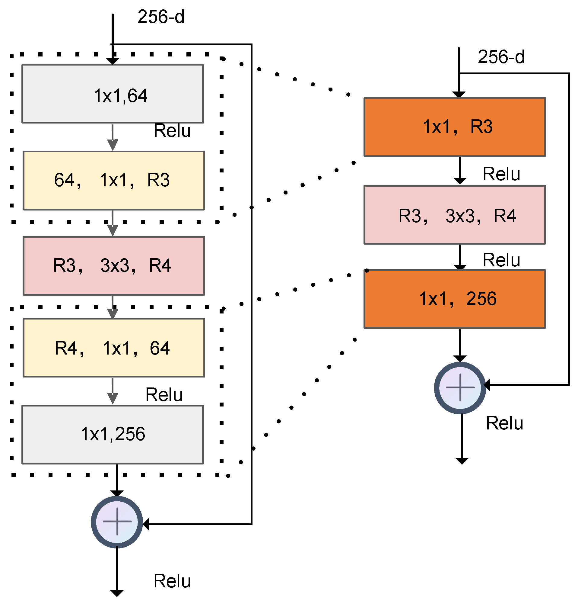
Despite the decomposition of the weight tensor and the reduction in the number of parameters, the layers in the bottleneck increased. These increased layers would lead to a longer inference time, which is not what we expected.
As shown in Figure 3, to decompose the weight tensors without increasing the convolution layers, we merged the two continuous pointwise convolution layers into a single layer. Then, we could obtain a decomposed module, named DecomResnet, that could be used to construct the compressed model.

3.3. Rank Selection

In this paper, the compression ratio (CR) indicated the number of parameters in the decomposed version compared to that of the original model. Moreover, the speedup ratio (SR) indicated the computing cost in the decomposed version compared to the original model.
C R = D 2 S T S R 3 + D 2 R 3 R 4 + T R 4
S R = D 2 S T H W S R 3 H W + D 2 R 3 R 4 H W + T R 4 H W
As shown in the compression ratio and speedup ratio definition equations, the ranks ( R 3 and R 4 ) are vital hyperparameters that regulate the computing and storage complexity of the compressed object detection model.
Although we sought to obtain the optimal ranks for the best approximation of the CNN object detection model, unfortunately, this was an NP-hard problem [38].
In our work, we adopted the VBMF method for the following reasons: First, this method can automatically find the noise variance and rank. Second, it can even provide a theoretical condition for perfect rank recovery. Third, libraries that can execute Tucker decomposition with the ranks chosen through this method are readily accessible, such as Tensorly. Finally, several works [16,31] have used this method and have achieved desirable results.
Variational Bayesian matrix factorization (VBMF) [37] has been proven to be an effective method for obtaining the suboptimal rank. This paper used the VBMF method for the mode-3 and mode-4 matricization of the kernel tensor, respectively, to obtain the ranks of Tucker decomposition ( R 3 and R 4 ).

3.4. Computation of Tensor Decomposition

Although Tucker decomposition is not unique to n-rank tensors, the problem can be solved by adding constraints. The HOSVD (high-order SVD) algorithm is a typical method for solving Tucker decomposition which first obtains the factor matrix for each mode through SVD decomposition then uses the projection of the tensor of each mode as the kernel tensor.
Although the HOSVD algorithm [39] can perform the Tucker decomposition of the tensor, it is not optimal for giving the best approximation. It is a good initialization for other iterative algorithms, such as high-order orthogonal iteration (HOOI) [15]. HOOI treats tensor decomposition as an optimization process and iterates continuously to obtain the decomposition result.
Suppose there is an Nth-order tensor. Then, the decomposition of the tensor could be formulated as the optimization problem as shown in Equation (11).
min S , A ( 1 ) , , A ( N ) X S ; A ( 1 ) , , A ( N )
which is subject to S R 1 × R 2 × × R N and A ( n ) I n × R n and in which each column is orthogonal.
The objective function could be rewritten in vectorized form as shown in Equation (12).
| X S ; A ( 1 ) , , A ( N ) | = V e c ( X ) ( A ( N ) A ( 1 ) ) V e c ( S ) = X 2 2 X , S ; A ( 1 ) , , A ( N ) + S ; A ( 1 ) , , A ( N ) 2 = X 2 2 X × 1 A × 2 ( 1 ) T × N A ( N ) T , S + S 2 = X 2 2 S , S + S 2
Then, it was straightforward that the square of the objective function could be written as Equation (13).
X S ; A ( 1 ) , , A ( N ) 2 = X 2 X × 1 A × 2 ( 1 ) T × N A ( N ) T 2
which is subject to A ( n ) I n × R n and in which each column is orthogonal.
Since X is a constant, minimizing Equation (13) was equivalent to maximizing A ( n ) T W , which could be expressed as Equation (14).
max A ( n ) T W s . t . W = X ( n ) ( A ( N ) A ( n + 1 ) A ( n 1 ) A ( 1 ) )
The solution could be obtained by using SVD and by using A ( n ) as the R n leading left singular value vector of W .

3.5. Training Method

Kossaifi et al. [40] pointed out that tensor contraction is a natural way to integrate tensor decomposition into a neural network as a differentiable layer. This technique is called the tensor contraction layer (TCL). Because of the backpropagation process of training, each decomposed layer needs to be differentiable.
As shown in equation (2), convolution kernel tensor K could be decomposed into a low-rank core, C R 1 × R 2 × R 3 × R 4 , and four factors, K ( 1 ) D × R 1 , K ( 2 ) D × R 2 , K ( 3 ) S × R 3 , and K ( 4 ) T × R 4 . Although Tucker decomposition was discussed in the context of four models, it can be generalized to N-way tensors as shown in Equation (15).
K C ; K ( 1 ) , K ( 2 ) , , K ( N )
The input and output feature maps were denoted as X B × I 0 × I 1 × × I N and Y B × O , respectively. B corresponds to the input samples, and O corresponds to the labels of each sample. Kernel tensor K I 0 × I 1 × × I N × O was decomposed under a fixed low rank ( R 0 , R N , R N + 1 ) . Then the convolution with the decomposed kernel tensor could be taken as tensor regression layers and could be written as Equation (16).
Y = X , K N + b subject   to   K = S ; K ( 0 ) , , K ( N + 1 )
S R 0 × × R N × R N + 1 ; K ( i ) I i × R i for each i in [ 0 N ] ; and K ( N + 1 ) O × R N + 1 .
The convolution function maps a tensor of size I 1 × × I N to space f I N + 1 with low-rank constraints. By using tensor unfolding [41], the partial derivatives for each factor could be obtained. For example, the partial derivatives for K ( 1 ) and K ( N + 1 ) could be expressed as formula (17) and formula (18), respectively.
( Y K ( 1 ) ) ( 1 ) = ( S ; I R 1 , K ( 2 ) , , K ( N + 1 ) ) ( N + 1 ) ( X ( 1 ) I R 1 ) T
( Y K ( N + 1 ) ) ( 1 ) = ( ( S ; K ( 1 ) , , K ( N ) , I R N + 1 ) ( N + 1 ) v e c ( X ) ) T I I N + 1
The Tucker decomposition differential for the kernel tensor could also be obtained in the same way as shown in formula (19).
( Y S ) ( 1 ) = K ( N + 1 ) v e c ( X ; ( K ( 1 ) ) T , , ( K ( N ) ) T ) T
From the above analysis, it can be seen that the decomposed components of the kernel tensor can be taken as neural network layers and that each layer is differentiable. The Tensorly [42] library was used to perform Tucker decomposition in this work.

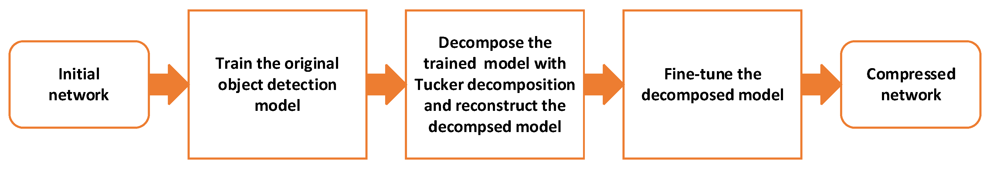
3.6. The Overall Procedure

As shown in Figure 4, our method for object detection model compression included the following steps:
Step 1:
Initialize RetinaNet with the pretrained model on ImageNet.
Step 2:
Train the object detection network model on the remote sensing dataset to obtain the trained model.
Step 3:
Obtain the ranks using the VBMF and decompose the trained model layer by layer using Tucker decomposition. Then, use the DecomResnet module to reconstruct the model.
Step 4:
Retrain the reconstructed model over multiple epochs.

4. Experiments

4.1. Datasets

Two datasets were used to evaluate the proposed method in our experiments. The first was the NWPU VHR-10 dataset [43], which contains ten categories. The second was the CAST-RS2 dataset constructed in this work. Some visualization results of samples and annotations of the CAST-RS2 dataset are shown in Figure 5.
In our actual mission, not all categories in the NWPU VHR-10 dataset had to be detected. To validate the performance of the decomposed model in our actual mission, we constructed the CAST-RS2 dataset, which contained only two types of objects, planes and ships.
The image samples came from two public datasets, DOTA [44] and HRSC2016 [45]. Since the HRSC dataset contains many ship objects and since the DOTA dataset is rich in scenes and has a large amount of data, we selected 1393 remote sensing images from these 2 datasets.
The process of constructing the dataset is described as follows: First, the plane and ship samples were selected from the DOTA and HRSC datasets. Second, the width and height of each object that was annotated in a sample image were multiplied to determine the size of each object in the selected images. The object size distribution of each class selected from the two datasets was then counted individually. Third, by scaling the images, the object size distribution of the corresponding categories in the two datasets was made to be almost comparable. Finally, the image was divided into 512 × 512 slices, and the slices that included objects were chosen as samples for the CAST-RS2 dataset.
There were 4032 annotated plane and ship objects in total. The 4032 annotated plane and ship objects were separated into 2 sets, with 2799 in the training set and 1233 in the test set. The three decomposed models were also assessed with this dataset.

4.2. Experimental Results

The operating system used in these experiments was 64-bit Ubuntu 18.04. The CPU was Intel (R) Core (TM) i7-6850K with six cores at 3.60 GHz, and the memory was 16 GB. The deep learning framework was Pytorch 1.6.0. CUDA 10.1 and cuDNN 7.6.3 were used. These models were trained on an NVIDIA TITAN Xp GPU. The momentum and weight decay parameters were set to 0.9 and 0.001, respectively. The object detection model was trained for 200 epochs.
In this work, the model that decomposed only the backbone was called Decom_b. The model that decomposed the backbone and the detection head was called Decom_bh. Additionally, the model that decomposed the backbone, the detection head, and the neck was called Decom_all.
In our experiments, we set up three sets of experiments for each dataset to evaluate the performance of the Decom_b, Decom_bh, and Decom_all models.

4.2.1. The Rank Produced through The VBMF Approach

In this work, RetinaNet was selected as the baseline. For the RetinaNet object detection model, the ranks produced through the VBMF approach are displayed in Table 1, Table 2 and Table 3. As shown in Equations (9) and (10), these ranks were vital hyperparameters used for Tucker decomposition. Each 3 × 3 convolution layer in the Resnet-50 backbone was decomposed with the ranks listed in Table 1. Each 3 × 3 convolution layer in the neck of RetinaNet was also decomposed with the ranks listed in Table 2. The classification network and regression network in the Retina head were also decomposed with ranks listed in Table 3.

4.2.2. Results for NWPU VHR-10 Dataset

As shown in Table 4, when only the backbone was decomposed, the AP (average precision) of the ship category, the ground track field category, and the harbor category improved by 2.4%, 1%, and 1.8%, respectively. The AP of other categories decreased, and the storage tank category had the largest performance drop of 4%. Compared to the baseline, the mAP (mean average precision) of Decom_b improved by 0.1%. It can be seen that, although the AP of some classes decreased, only the backbone compression had almost no effect on the mAP of the model.
When the backbone and the detection head were compressed, the mAP of Decom_bh decreased by only 1.1%. The detection results showed that the AP of the bridge category decreased the most, as it decreased by 8.2%, followed by the basketball court category, which decreased by 6.40%, and the storage tank and tennis court categories, which decreased by 3.1% and 3.2%, respectively.
The AP of the ship category and the harbor category improved by 2.2% and 2.9%, respectively. In the NWPU VHR-10 dataset, bridges and basketball courts are large objects, and storage tanks and tennis courts are smaller objects. We could draw an imprecise conclusion that, although the mAP of Decom_bh decreased slightly, there was an impact on the large and small objects and almost no impact on the AP of other classes. Of course, this conclusion was not verified, and we will continue to verify this conjecture in future work.
When all parts of the object detection model, including the neck, were compressed, the mAP of the model decreased by 5.30%, which was mainly caused by the AP loss in the bridge category. The AP of the court category also decreased by 6.2%. It can be seen that the mAP of Decom_all decreased and that the AP of some categories decreased significantly, such as the bridge category. It is worth noting that the performance of the ship category improved when both the backbone and the detection head were decomposed, but its performance decreased by 6.7% when the neck was decomposed.
Table 5 shows the compression ratio and speedup ratio when different parts of the object detection model were decomposed.
As shown in Table 5, the number of parameters could be reduced by a factor of 1.91, and the computational cost could be reduced by 1.36 when only the backbone was compressed. The mAP did not decrease at this time, even with a 0.1% improvement.
When both the backbone and the detection head were decomposed, the number of parameters decreased by 2.58 times, the computational cost decreased by 4.37 times, and the mAP only reduced by 1.1%. When the backbone, the head, and the neck were decomposed simultaneously, the number of model parameters was compressed by 4.44 times, the acceleration ratio increased by 5.71 times, and the mAP decreased by 5.3%.
Therefore, we could conclude that, although there was no mAP loss for Decom_b, its compression ratio and acceleration ratio were also relatively small. Decom_bh had a slight loss in mAP, but the compression ratio and acceleration ratio were also greatly improved. Decom_all could achieve the optimal compression and maximum acceleration ratios, but it also had a more considerable mAP loss. When the storage and computational resources are not very stringent, we could consider decomposing only the backbone and the detection head to ensure performance. When there are performance demands, we could decompose each part of the model to obtain the optimal compression ratio and acceleration ratio.
PR curves for the three decomposition modes and baseline mode, which were tested on the NWPU VHR-10 dataset, are shown in Figure 6.
The precision of Decom_b was comparable to that of the baseline. The precision of Decom_bh was slightly lower than that of the baseline, and the recall was slightly higher than that of the baseline. The precision of Decom_all was lower than that of the baseline.
Figure 7 shows the PR curves of Decom_all for each category, which were tested on the NWPU VHR-10 dataset.
It can be seen that, although the mAP only decreased by 5.3%, the accuracy of some categories decreased severely, such as the bridge category, which had a decrease of 25.3%. Moreover, the accuracy of the ship, storage tank, tennis court, and basketball court categories showed a significant decline.
As shown in Figure 8, the 3 decomposition models converged after 120 epochs. The loss curves of the Decom_b model and the Decom_bh model were very close after 120 epochs, which indicated that the difference between these 2 models tested on this dataset was minimal. The loss curve of the Decom_all model was slightly higher than the loss curves of the other two models. However, it was still in the convergence state.

4.2.3. Results for The CAST-RS2 Dataset

In some missions, not so many categories need to be detected. For example, only the ship and the plane categories needed to be detected in our mission. To satisfy the requirements of our mission, we also evaluated the proposed method on the CAST-RS2 dataset. The evaluation results of the three decomposed models are shown in Table 6.
Table 7 shows the compression ratio and acceleration ratio of the three decomposed models tested on the CAST-RS2 dataset. They were slightly different from those that were tested on the NWPU VHR-10 dataset.
The mAP of the baseline was 95.3%. The mAP of Decom_b improved slightly by 0.6%. The mAP of Decom_bh was 95.4%. These results demonstrated that Decom_b and Decom_bh had no mAP loss when tested on the CAST-RS2 dataset. The mAP of Decom_all decreased by 1.9%, mainly due to the higher AP loss in the ship category.
As shown in Figure 9, the precision of Decom_b and that of Decom_bh were slightly different from the baseline. However, the precision of Decom_all was slightly lower than that of the baseline. It still reached 93.4%, which met our mission requirements.
Figure 10 shows the PR curves of the Decom_all model for the ship and plane categories tested on the CAST-RS2 dataset. We could draw a similar conclusion that the proposed method worked well on the CAST-RS2 dataset and that the decomposed model had good performance in terms of accuracy and recall.
As shown in Figure 11, the baseline and the 3 decomposed models converged when trained for more than 100 epochs. Although the loss of the three decomposed models was slightly more significant than the baseline model, it was very close to the baseline.

4.2.4. Comparison with Other Compression Methods

Some similar state-of-the-art works conduct experiments on the Resnet-50 classification task, and we compared these methods with our method. For a fair comparison, we migrated the proposed approach to the classification task and evaluated it on the ImageNet dataset. The decomposed Resnet-50 was trained on the ImageNet dataset for 200 epochs using stochastic gradient descent with a learning rate of 0.0001, weight decay of 0.0005, and momentum of 0.9. The original network achieved a top-1 accuracy of 76.41% and a top-5 accuracy of 92.64%. The decomposed network achieved a top-1 accuracy of 75.65% and a top-5 accuracy of 92.07%.
To quantitatively evaluate the proposed method, we compared it with nine low-rank decomposition methods with respect to model compression on Resnet-50, including CC [46], Stable [47], TRP [48], HODEC [49], CP-TPM [50], LTD [51], HT-2 [32], GKPD [33], and LRDKT [52].
The compression ratio (CR), speedup ratio (SR), and performance loss (PL) were compared. Most low-rank decomposition methods were verified on AlexNet or VGG, but these models were unsuitable for the onboard object detection task.
Here, performance loss refers to Top-1 accuracy loss with respect to the classification task and mAP loss with respect to the object detection task.
As shown in Table 8, the proposed method achieved the most significant compression and speedup ratios compared to other SOTA methods.
The proposed method achieved the best compression ratio for the classification task when tested on the ImageNet dataset compared to the similar methods mentioned above. It could achieve up to 4.25 times the compression with merely a 0.57% decrease in Top-1 accuracy.
ThiNet-30 achieved marginally higher SR at the cost of a more significant drop in accuracy, and it had a lower CR.
HODEC achieved a slight increase in Top-1 accuracy, but our method had a more significant SR.
In the case of CC (C = 0.5), it had a PL that was similar to our method, but our method had a larger CR and SR. In the case of CC (C = 0.6), all its metrics were worse than those of our method.
Compared to Stable, TRP, CP-TPM, LTD, GKPD, ThiNet-50, and ThiNet-70, our method outperformed these methods in all the metrics.
The recently published HT-2 had a comparable SR, but our method had a more significant CR and a smaller PL.
Compared to LRDKT, our method obtained a significantly lower accuracy drop with a slightly larger CR.
We also compared the proposed method with state-of-art algorithms across tasks and datasets. For instance, CC achieved a 2.42 compression ratio and a 2.68 speedup ratio. Our method achieved nearly two times those of CC with a slightly more significant performance loss.
Our method obtained a compression ratio comparable to LRDKT, but the speedup ratio of our approach was 2.54 times that of LRDKT with a slightly smaller performance loss.
Compared with HODEC, the speedup ratio of our method was 2.06 times higher, but there was a 0.31 performance improvement with HODEC and a slight performance decrease with our approach.
Compared with Stable, TRP, and LTD, the proposed method achieved the best performance, compression ratio, and speedup ratio.
Compared with ThiNet-30, the speedup ratio of our method was 1.63 times higher, and the compression ratio was 1.51 times higher with a 0.84% greater performance loss.

4.2.5. Ablation Study

In this section, an ablation study was performed to illustrate how the selection of rank affects performance, the number of parameters, and the cost of computing.
This work used VBMF to obtain the ranks of Tucker decomposition ( R 3 , R 4 ) . Scaling factor α was used to implement the scaling of the rank acquired through the VBMF method in ablation experiments to study the performance, parameters, and computing consumption of the model for ranks larger than and less than the VBMF rank, respectively. In Equation (20), the scaled ranks are displayed.
R i = min ( α × R i I i ) i = 3 , 4
Table 9 shows the results of the decomposition model Decom_all tested on the NWPU VHR-10 dataset when α is 0.75, 0.875, 1.125, and 1.25, respectively. The PR curves are shown in Figure 12.
As shown in Table 9, when the rank decreased by 1/8, the number of parameters decreased by 1.1 M, the computing cost decreased by 0.5 GMac, and the mAP decreased by 10.7. When the rank decreased by 1/4, the number of parameters decreased by 3.02 M, the computing cost decreased by 2.69 Gmac, and the mAP decreased by 17.4.
When the rank increased by 1/8, the number of parameters increased by 2.28 M, and the computing cost increased by 3.85 Gmac. When the rank increased by 1/4, the number of parameters increased by 9.07 M, and the computing cost increased by 7.45 Gmac.
We could conclude the following three points:
(1)
When Tucker decomposition was used to decompose the object detection model, the larger the rank, the larger the number of parameters and the computing cost, and the better the performance of the decomposed model and vice versa. However, there was no evidence of a linear link between the variance in rank and the variation in the number of parameters, computing cost, or mAP.
(2)
When the rank obtained through the VBMF method was reduced, its performance appeared to drop significantly, although the number of parameters and the computational cost was reduced. Undoubtedly, we could find the optimal scaling factor by using a more refined scaling factor, such as 1/16, 1/32, etc., so that the model performance decrease matches the complexity decrease. However, this would make the time cost significantly higher.
(3)
When the rank obtained using VBMF increased, although the model’s performance was improved, the number of parameters and the computation cost appeared to increase significantly. We could also find the optimal scaling factor by using a more refined scaling factor so that the improvement in model performance matches the increase in model complexity.
It can be seen that using the VBMF method to obtain the rank does not necessarily create the best balance between the complexity and performance of the decomposition model. However, we can use a relatively low-cost method in engineering applications to solve the problem.

5. Discussion

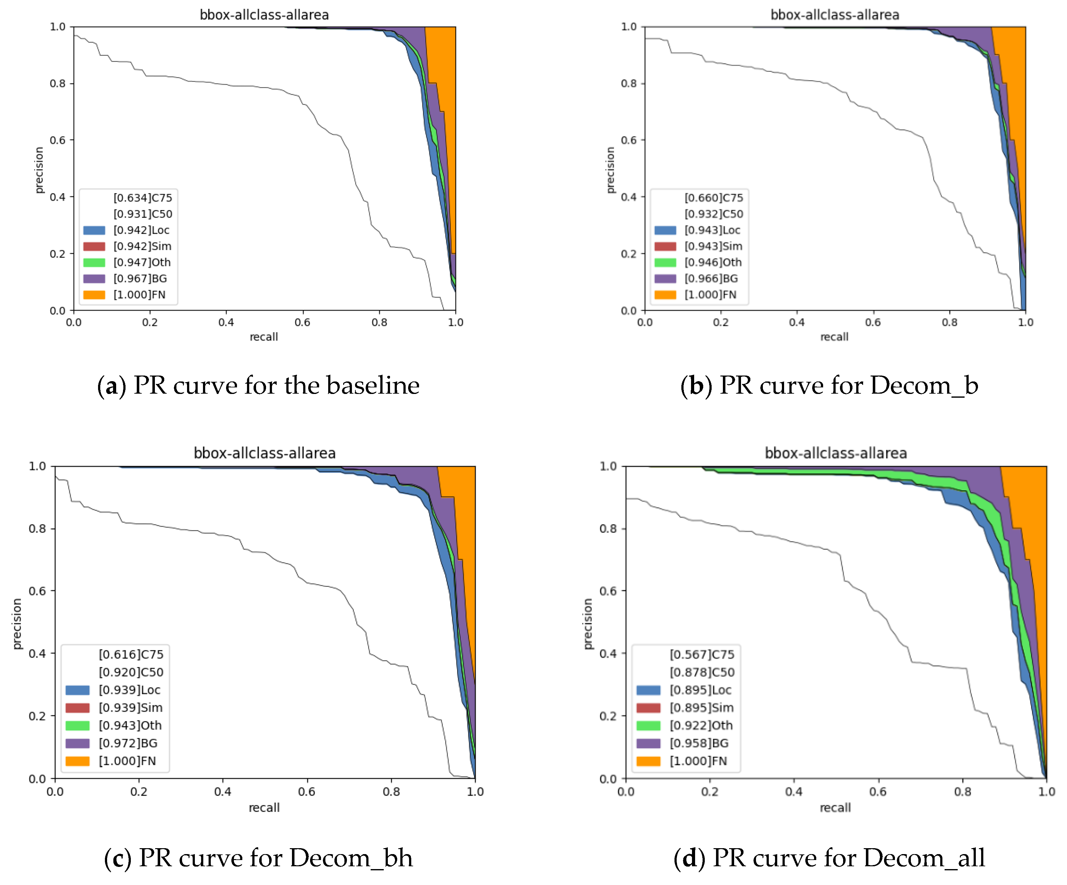
The experiments’ results demonstrated that the proposed method achieved a performance comparable to that of other methods. It worked well when tested on both our actual application mission CAST-RS2 dataset and the public NWPU VHR-10 dataset. The compression ratio and speedup ratio reached those of the SOTA methods with a slight performance decrease.
Currently, most CNN model compression algorithms based on low-rank decomposition have been developed and evaluated for the classification task. Still, our method was developed for the remote sensing image object detection task, which is increasingly in demand for onboard applications. As far as we know, this work is the first low-rank-based CNN model compression work to be aimed at onboard object detection algorithm deployment.
The advantages of the proposed method can be summarized as follows:
First, the number of CNN layers of the decomposed model does not increase. Unlike the previous works [30,31], the decomposition model in this paper did not increase the number of layers of the CNN model. In practical applications, an increased number of convolutional layers in the model decomposition process consumes computational resources and increases the computation time. The increased convolutional layers may become a computational bottleneck as the convolutional model is computed layer by layer. This feature is essential for onboard applications.
Second, each part of the object detection model can be decomposed with the same method. Only the backbone has been decomposed in previous works, such as in Resnet or VGG, but each part of the CNN object detection model was decomposed with the same method, including the neck and detection head.
Third, The VBMF method was adopted for rank selection, and it is an easily accessible and highly reproducible method. These features are more important for engineering applications than a group of optimal ranks.
The VBMF rank selection is also a drawback of the proposed method. The performance loss may be higher than that of its optimal counterpart. The results of the ablation study showed that we can obtain more optimal ranks by multiplying a scaling factor by the suboptimal ranks, but it is a time-consuming procedure.
The primary reasons that prevent CNNs from being deployed onboard are that hardware that predates the algorithms has insufficient performance and that many CNN models are computationally intensive. Our goal was to attempt to obtain a scalable and general approach that could reduce the complexity of CNNs. The experimental results demonstrated that the proposed method can be applied in our real mission to deploy an object detector on a satellite.
In addition, there are some other potential real-world uses. One example is represented by a CNN-based cloud detection algorithm, which is a typical mission for Earth observation satellites. The proposed method can be used to compress a CNN cloud detector deployed on a satellite and to select the images eligible for transmission to the ground to reduce the amount of data to be transmitted to the ground. Another example is represented by the CNN-based instance segmentation and object detection algorithms deployed on airplanes or on satellites to process the images of synthetic aperture radars (SARs). These CNN-based SAR image processors can also be compressed using the proposed method.

6. Conclusions

In this work, we proposed an object detection model compression method based on Tucker decomposition to solve the problem of the high storage and computing complexity of the CNN-based object detection model that was deployed onboard. The proposed method can effectively achieve the compression of the object detection model with Resnet as the backbone. The compression ratio reached 4.44, and the speedup ratio reached 5.71. The mAP only decreased by 1.9% when tested on the CAST-RS2 dataset and by 5.3% when tested on the NWPU VHR-10 dataset.
Although the proposed method was only evaluated on the RetinaNet, it is a general low-rank decomposition compression method that can decompose other object detection models. In addition, although the method was proposed for object detection tasks on satellites, it can also be applied to other mobile application tasks, such as object detection and classification on mobile devices.
Note that adequate experiments were conducted on the CAST-RS2 and the NWPU VHR-10 datasets. Although the experimental results showed that the proposed method effectively achieved model compression, the VBMF method was employed to determine the ranks of Tucker decomposition, which is not an optimal rank selection method. Other methods could be tried to obtain optimal ranks in future works. In addition, the proposed method could be combined with other compression methods, such as pruning or quantization, to further improve the compression ratio.

Author Contributions

Conceptualization, L.H. and Y.L.; methodology, D.J., Y.Z. (Yanning Zhang), and Q.Z.; software, L.H., J.W., and B.L.; validation, L.H. and J.W.; formal analysis, Q.Z. and Y.Z. (Yi Zhang); investigation, J.L. and P.W.; resources, L.H.; data curation, J.W. and J.L.; writing—original draft preparation, L.H.; writing—review and editing, Q.Z.; visualization, J.W. and H.F.; supervision, Y.L.; project administration, Q.Z.; funding acquisition, L.H. and H.F. All authors have read and agreed to the published version of the manuscript.

Funding

This research was funded by the National Key Research and Development Program of China (2020YFB1808003), Shaanxi Provincial Key R&D Program, China (2023-GHZD-02), the Innovation Foundation of CAS (Y20-JTKJCX-02), the National Key Laboratory Foundation of China (6142411432107), and the Sustained Supported Foundation of the National Key Laboratory of Science and Technology on Space Microwave (HTKJ2022KL504007).

Data Availability Statement

The NWPU-VHR-10 dataset and the DIOR dataset presented in this study are available at Baidupan at doi:10.1016/j.isprsjprs.2014.10.002, reference number [37].

Acknowledgments

The authors would like to express gratitude to Gong Cheng from Northwestern Polytechnical University for providing remote sensing objection dataset NWPU VHR-10. The authors would also like to thank the anonymous reviewers for their thoughtful comments and helpful suggestions.

Conflicts of Interest

The authors declare no conflict of interest.

References

  1. Yun, J.-S.; Park, S.-H.; Yoo, S.B. Infusion-Net: Inter- and Intra-Weighted Cross-Fusion Network for Multispectral Object Detection. Mathematics 2022, 10, 3966. [Google Scholar] [CrossRef]
  2. Wu, D.; Song, H.; Fan, C. Object Tracking in Satellite Videos Based on Improved Kernel Correlation Filter Assisted by Road Information. Remote Sens. 2022, 14, 4215. [Google Scholar] [CrossRef]
  3. Liu, B.; Hu, J.; Bi, X.; Li, W.; Gao, X. PGNet: Positioning Guidance Network for Semantic Segmentation of Very-High-Resolution Remote Sensing Images. Remote Sens. 2022, 14, 4219. [Google Scholar] [CrossRef]
  4. Giuffrida, G.; Diana, L.; de Gioia, F.; Benelli, G.; Meoni, G.; Donati, M.; Fanucci, L. CloudScout: A Deep Neural Network for On-Board Cloud Detection on Hyperspectral Images. Remote Sens. 2020, 12, 2205. [Google Scholar] [CrossRef]
  5. Furano, G.; Meoni, G.; Dunne, A.; Moloney, D.; Ferlet-Cavrois, V.; Tavoularis, A.; Byrne, J.; Buckley, L.; Psarakis, M.; Voss, K.-O.; et al. Towards the Use of Artificial Intelligence on the Edge in Space Systems: Challenges and Opportunities. IEEE Aerosp. Electron. Syst. Mag. 2020, 35, 44–56. [Google Scholar] [CrossRef]
  6. Kothari, V.; Liberis, E.; Lane, N.D. The final frontier: Deep learning in space. In Proceedings of the 21st International Workshop on Mobile Computing Systems and Applications, Austin, TX, USA, 3–4 March 2020; pp. 45–49. [Google Scholar]
  7. Denby, B.; Lucia, B. Orbital edge computing: Nanosatellite constellations as a new class of computer system. In Proceedings of the Twenty-Fifth International Conference on Architectural Support for Programming Languages and Operating Systems, Lausanne, Switzerland, 16–20 March 2020; pp. 939–954. [Google Scholar]
  8. Cheng, G.; Han, J. A survey on object detection in optical remote sensing images. ISPRS J. Photogramm. Remote Sens. 2016, 117, 11–28. [Google Scholar] [CrossRef]
  9. Shen, H.; Pan, W.D.; Wu, D. Predictive Lossless Compression of Regions of Interest in Hyperspectral Images with No-Data Regions. IEEE Trans. Geosci. Remote Sens. 2017, 55, 173–182. [Google Scholar] [CrossRef]
  10. Zhu, X.X.; Tuia, D.; Mou, L.; Xia, G.-S.; Zhang, L.; Xu, F.; Fraundorfer, F. Deep Learning in Remote Sensing: A Comprehensive Review and List of Resources. IEEE Geosci. Remote Sens. Mag. 2017, 5, 8–36. [Google Scholar] [CrossRef]
  11. Furano, G.; Menicucci, A. Roadmap for onboard processing and data handling systems in space. In Dependable Multicore Architectures at Nanoscale; Springer: Berlin/Heidelberg, Germany, 2018; pp. 253–281. [Google Scholar]
  12. Lentaris, G.; Maragos, K.; Stratakos, I.; Papadopoulos, L.; Papanikolaou, O.; Soudris, D.; Lourakis, M.; Zabulis, X.; Gonzalez-Arjona, D.; Furano, G. High-Performance Embedded Computing in Space: Evaluation of Platforms for Vision-Based Navigation. J. Aerosp. Inf. Syst. 2018, 15, 178–192. [Google Scholar] [CrossRef]
  13. Benelli, G.; Meoni, G.; Fanucci, L. A low power keyword spotting algorithm for memory constrained embedded systems. In Proceedings of the 2018 IFIP/IEEE International Conference on Very Large Scale Integration (VLSI-SoC), Verona, Italy, 10 October 2018; pp. 267–272. [Google Scholar]
  14. Rakhuba, M.; Oseledets, I.; Lempitsky, V.; Lebedev, V.; Ganin, Y. Speeding-up convolutional neural networks using fine-tuned cp-decomposition. arXiv 2014, arXiv:1412.6553. [Google Scholar]
  15. Kolda, T.G.; Bader, B.W. Tensor Decompositions and Applications. SIAM Rev. 2009, 51, 455–500. [Google Scholar] [CrossRef]
  16. Kim, Y.-D.; Park, E.; Yoo, S.; Choi, T.; Yang, L.; Shin, D. Compression of deep convolutional neural networks for fast and low power mobile applications. arXiv 2015, arXiv:1511.06530. [Google Scholar]
  17. Tucker, L.R. Some mathematical notes on three-mode factor analysis. Psychometrika 1966, 31, 279–311. [Google Scholar] [CrossRef]
  18. Simonyan, K.; Zisserman, A. Very Deep Convolutional Networks for Large-Scale Image Recognition. arXiv 2014, arXiv:1409.1556. [Google Scholar]
  19. Krizhevsky, A.; Sutskever, I.; Hinton, G.E. ImageNet classification with deep convolutional neural networks. Commun. ACM 2017, 60, 84–90. [Google Scholar] [CrossRef]
  20. He, K.; Zhang, X.; Ren, S.; Sun, J. Deep Residual Learning for Image Recognition. In Proceedings of the 2016 IEEE Conference on Computer Vision and Pattern Recognition (CVPR), Las Vegas, NV, USA, 27–30 June 2016. [Google Scholar]
  21. Park, W.; Kim, D.; Lu, Y.; Cho, M. Relational Knowledge Distillation. In Proceedings of the 2019 IEEE/CVF Conference on Computer Vision and Pattern Recognition (CVPR), Long Beach, CA, USA, 15–20 June 2019. [Google Scholar]
  22. Luo, J.-H.; Wu, J.; Lin, W. Thinet: A filter level pruning method for deep neural network compression. In Proceedings of the IEEE international conference on computer vision, Venice, Italy, 22–29 October 2017; pp. 5058–5066. [Google Scholar]
  23. Zhou, S.-C.; Wang, Y.-Z.; Wen, H.; He, Q.-Y.; Zou, Y.-H. Balanced Quantization: An Effective and Efficient Approach to Quantized Neural Networks. J. Comput. Sci. Technol. 2017, 32, 667–682. [Google Scholar] [CrossRef]
  24. Rabanser, S.; Shchur, O.; Günnemann, S. Introduction to Tensor Decompositions and their Applications in Machine Learning. arXiv 2017, arXiv:1711.10781. [Google Scholar]
  25. Iandola, F.N.; Han, S.; Moskewicz, M.W.; Ashraf, K.; Dally, W.J.; Keutzer, K. SqueezeNet: AlexNet-level accuracy with 50x fewer parameters and <0.5MB model size. arXiv 2016, arXiv:1602.07360. [Google Scholar]
  26. Szegedy, C.; Wei, L.; Jia, Y.; Sermanet, P.; Reed, S.; Anguelov, D.; Erhan, D.; Vanhoucke, V.; Rabinovich, A. Going deeper with convolutions. In Proceedings of the 2015 IEEE Conference on Computer Vision and Pattern Recognition (CVPR), Boston, MA, USA, 7–12 June 2015. [Google Scholar]
  27. Denil, M.; Shakibi, B.; Dinh, L.; Ranzato, M.; de Freitas, N. Predicting parameters in deep learning. In Proceedings of the Advances in Neural Information Processing Systems, Lake Tahoe, NV, USA, 5–10 December 2013; Volume 26. [Google Scholar]
  28. Garipov, T.; Podoprikhin, D.; Novikov, A.; Vetrov, D. Ultimate tensorization: Compressing convolutional and FC layers alike. arXiv 2016, arXiv:1611.03214. [Google Scholar]
  29. Fonał, K.; Zdunek, R. Distributed and randomized tensor train decomposition for feature extraction. In Proceedings of the 2019 International Joint Conference on Neural Networks (IJCNN), Budapest, Hungary, 14–19 July 2019; pp. 1–8. [Google Scholar]
  30. Huang, J.; Sun, W.; Huang, L.; Chen, S. Deep compression with low rank and sparse integrated decomposition. In Proceedings of the 2019 IEEE 7th International Conference on Computer Science and Network Technology (ICCSNT), Dalian, China, 19–20 October 2019; pp. 289–292. [Google Scholar]
  31. Elhoushi, M.; Tian, Y.H.; Chen, Z.; Shafiq, F.; Li, J.Y. Accelerating Training using Tensor Decomposition. arXiv 2019, arXiv:1909.05675. [Google Scholar]
  32. Gabor, M.; Zdunek, R. Compressing convolutional neural networks with hierarchical Tucker-2 decomposition. Appl. Soft Comput. 2023, 132, 109856. [Google Scholar] [CrossRef]
  33. Hameed, M.G.A.; Tahaei, M.S.; Mosleh, A.; Nia, V.P. Convolutional neural network compression through generalized Kronecker product decomposition. In Proceedings of the AAAI Conference on Artificial Intelligence, Washington, DC, USA, 7–14 February 2022; pp. 771–779. [Google Scholar]
  34. Saha, A.; Ram, K.S.; Mukhopadhyay, J.; Das, P.P.; Patra, A. Fitness based layer rank selection algorithm for accelerating CNNs by candecomp/parafac (CP) decompositions. In Proceedings of the 2019 IEEE International Conference on Image Processing (ICIP), Taipei, Taiwan, 22–25 September 2019; pp. 3402–3406. [Google Scholar]
  35. Jaderberg, M.; Vedaldi, A.; Zisserman, A. Speeding up Convolutional Neural Networks with Low Rank Expansions. arXiv 2014, arXiv:1405.3866. [Google Scholar]
  36. Yin, M.; Phan, H.; Zang, X.; Liao, S.; Yuan, B. Batude: Budget-aware neural network compression based on tucker decomposition. In Proceedings of the AAAI Conference on Artificial Intelligence, Washington, DC, USA, 7–14 February 2023; pp. 8874–8882. [Google Scholar]
  37. Nakajima, S.; Sugiyama, M.; Babacan, S.D.; Tomioka, R. Global analytic solution of fully-observed variational Bayesian matrix factorization. J. Mach. Learn. Res. 2013, 14, 1–37. [Google Scholar]
  38. Bai, Z.; Li, Y.; Woźniak, M.; Zhou, M.; Li, D. DecomVQANet: Decomposing visual question answering deep network via tensor decomposition and regression. Pattern Recognit. 2021, 110, 107538. [Google Scholar] [CrossRef]
  39. Ahmadi-Asl, S.; Abukhovich, S.; Asante-Mensah, M.G.; Cichocki, A.; Phan, A.H.; Tanaka, T.; Oseledets, I. Randomized Algorithms for Computation of Tucker Decomposition and Higher Order SVD (HOSVD). IEEE Access 2021, 9, 28684–28706. [Google Scholar] [CrossRef]
  40. Kossaifi, J.; Khanna, A.; Lipton, Z.; Furlanello, T.; Anandkumar, A. Tensor contraction layers for parsimonious deep nets. In Proceedings of the IEEE Conference on Computer Vision and Pattern Recognition Workshops, Honolulu, HI, USA, 21–26 July 2017; pp. 26–32. [Google Scholar]
  41. Kossaifi, J.; Lipton, Z.C.; Kolbeinsson, A.; Khanna, A.; Furlanello, T.; Anandkumar, A. Tensor regression networks. J. Mach. Learn. Res. 2020, 21, 4862–4882. [Google Scholar]
  42. Kossaifi, J.; Panagakis, Y.; Anandkumar, A.; Pantic, M. TensorLy: Tensor Learning in Python. J. Mach. Learn. Res. 2019, 20, 1–6. [Google Scholar]
  43. Cheng, G.; Han, J.; Zhou, P.; Guo, L. Multi-class geospatial object detection and geographic image classification based on collection of part detectors. ISPRS J. Photogramm. Remote Sens. 2014, 98, 119–132. [Google Scholar] [CrossRef]
  44. Xia, G.-S.; Bai, X.; Ding, J.; Zhu, Z.; Belongie, S.; Luo, J.; Datcu, M.; Pelillo, M.; Zhang, L. DOTA: A Large-Scale Dataset for Object Detection in Aerial Images. In Proceedings of the IEEE Conference on Computer Vision and Pattern Recognition (CVPR), Salt Lake City, UT, USA, 18–23 June 2018. [Google Scholar]
  45. Liu, Z.; Wang, H.; Weng, L.; Yang, Y. Ship Rotated Bounding Box Space for Ship Extraction From High-Resolution Optical Satellite Images With Complex Backgrounds. IEEE Geosci. Remote Sensing Lett. 2016, 13, 1074–1078. [Google Scholar] [CrossRef]
  46. Li, Y.; Lin, S.; Liu, J.; Ye, Q.; Wang, M.; Chao, F.; Yang, F.; Ma, J.; Tian, Q.; Ji, R. Towards Compact CNNs via Collaborative Compression. In Proceedings of the IEEE/CVF Conference on Computer Vision and Pattern Recognition (CVPR), Nashville, TN, USA, 20–25 June 2021; pp. 6438–6447. [Google Scholar]
  47. Phan, A.-H.; Sobolev, K.; Sozykin, K.; Ermilov, D.; Gusak, J.; Tichavsk, P.; Glukhov, V.; Oseledets, I.; Cichocki, A. Stable low-rank tensor decomposition for compression of convolutional neural network. In Proceedings of the European Conference on Computer Vision, Glasgow, UK, 23–28 August 2020; pp. 522–539. [Google Scholar]
  48. Xu, Y.; Li, Y.; Zhang, S.; Wen, W.; Wang, B.; Qi, Y.; Chen, Y.; Lin, W.; Xiong, H. TRP: Trained Rank Pruning for Efficient Deep Neural Networks. arXiv 2020, arXiv:2004.14566. [Google Scholar]
  49. Yin, M.; Sui, Y.; Yang, W.; Zang, X.; Gong, Y.; Yuan, B. HODEC: Towards Efficient High-Order DEcomposed Convolutional Neural Networks. In Proceedings of the IEEE/CVF Conference on Computer Vision and Pattern Recognition, New Orleans, LA, USA, 18–24 June 2022; pp. 12299–12308. [Google Scholar]
  50. Astrid, M.; Lee, S.-I. Cp-decomposition with tensor power method for convolutional neural networks compression. In Proceedings of the 2017 IEEE International Conference on Big Data and Smart Computing (BigComp), Jeju Island, People Republic of Korea, 13–16 February 2017; pp. 115–118. [Google Scholar]
  51. Chu, B.-S.; Lee, C.-R. Low-rank Tensor Decomposition for Compression of Convolutional Neural Networks Using Funnel Regularization. arXiv 2021, arXiv:2112.03690. [Google Scholar]
  52. Lin, S.; Ji, R.; Chen, C.; Tao, D.; Luo, J. Holistic CNN compression via low-rank decomposition with knowledge transfer. IEEE Trans. Pattern Anal. Mach. Intell. 2018, 41, 2889–2905. [Google Scholar] [CrossRef] [PubMed]
Figure 1. Tucker decomposition and the proposed DecomResnet. (1) 256-d in the figure means that the input feature has 256 channels. The three elements in each module stand for the channel number of the input feature map, the convolution size, and the channel number of the output feature map, respectively. For example, “1 × 1, 64” in the top module stands for a convolution size of 1 × 1 with 256 input and 64 output channels. “1 × 1, 256” in the bottom module stands for a convolution size of 1 × 1 with 256 output channels. (2) “R3, 3 × 3, R4” stands for a convolution size of 3 × 3 with R3 input channels and R4 output channels. R3 and R4 are the ranks of Tucker decomposition.
Mathematics 11 00856 g001
Figure 2. RetinaNet object detection model.
Mathematics 11 00856 g002
Figure 3. DecomResnet based on Tucker decomposition. (1) 256-d in this figure means the input feature has 256 channels. The three elements in each module stand for the channel number of the input feature map, the convolution size, and the channel number of the output feature map, respectively. For example, “1 × 1, 64” in the top module stands for a convolution size of 1 × 1 with 256 input and 64 output channels. “1 × 1, 256” in the bottom module stands for a convolution size of 1 × 1 with 256 output channels. (2) “R3, 3 × 3, R4” stands for a convolution size of 3 × 3 with R3 input channels and R4 output channels. R3 and R4 are the ranks of Tucker decomposition.
Mathematics 11 00856 g003
Figure 4. Flowchart of the model compression procedure.
Mathematics 11 00856 g004
Figure 5. Visualization results of samples and annotations of the CAST-RS2 dataset containing the plane and ship categories.
Mathematics 11 00856 g005
Figure 6. All class PR curves for the three decomposition modes and baseline mode tested on the NWPU VHR-10 dataset.
Mathematics 11 00856 g006
Figure 7. The PR curves for Decom_all tested on the NWPU VHR-10 dataset.
Mathematics 11 00856 g007aMathematics 11 00856 g007b
Figure 8. The loss curves of the baseline and the three decomposed models tested on the NWPU VHR-10 dataset.
Mathematics 11 00856 g008
Figure 9. Average PR curves for baseline and all classes of the three decomposed models tested on the CAST-RS2 dataset.
Mathematics 11 00856 g009
Figure 10. The PR curves for Decom_all and baseline tested on the CAST-RS2 dataset.
Mathematics 11 00856 g010
Figure 11. The loss curves of the baseline and the three decomposed models tested on the CAST-RS2 dataset.
Mathematics 11 00856 g011
Figure 12. The PR curves for Decom_all tested on the NWPU VHR-10 dataset when α is 0.75, 0.875, 1.125, and 1.25.
Mathematics 11 00856 g012
Table 1. The ranks of Tucker decomposition ( R 3 and R 4 ) for the backbone of RetinaNet.
BackboneR3R4
Conv1228
Stage 1   Bottleneck 0 conv 23838
Stage 1   Bottleneck 1 conv 23025
Stage 1 Bottleneck 2 conv 22324
Stage 2 Bottleneck 0 conv 25054
Stage 2 Bottleneck 1 conv 27466
Stage 2 Bottleneck 2 conv 25352
Stage 2 Bottleneck 3 conv 24642
Stage 3 Bottleneck 0 conv 2106106
Stage 3 Bottleneck 1 conv 210696
Stage 3 Bottleneck 2 conv 29389
Stage 3 Bottleneck 3 conv 28479
Stage 3 Bottleneck 4 conv 27773
Stage 3 Bottleneck 5 conv 28375
Stage 4 Bottleneck 0 conv 2202192
Stage 4 Bottleneck 1 conv 2188152
Stage 4 Bottleneck 2 conv 2269251
Table 2. The ranks of Tucker decomposition ( R 3 and R 4 ) for the neck of RetinaNet.
NeckR3R4
FPN conv 011
FPN conv 1256256
FPN conv 211
FPN conv 312
FPN conv 4256256
Table 3. The ranks of Tucker decomposition ( R 3 and R 4 ) for the head of RetinaNet.
HeadR3R4
bbox_head cls_conv 01010
bbox_head cls_conv 1119
bbox_head cls_conv 21011
bbox_head cls_conv 31214
bbox_head reg_conv 067
bbox_head reg_conv 166
bbox_head reg_conv 278
bbox_head reg_conv 3811
retina_cls conv2019
retina_reg conv1413
Table 4. Detection AP (%) comparison of different algorithms tested on NWPU-VHR-10 dataset. AP loss in this table is the AP loss of Decom_all with respect to baseline.
BaselineDecom_bDecom_bhDecom_allAP Loss
Airplane97.9%98.0%98.3%97.8%0.10%
Ship89.2%91.6%91.4%82.5%6.70%
Storage tank96.6%92.6%93.5%88.6%8.00%
Baseball diamond99.2%97.7%98.1%97.2%2.00%
Tennis court91.0%90.2%87.8%84.8%6.20%
Basketball court99.2%94.0%92.8%92.0%7.20%
Ground track field94.9%95.9%94.9%93.2%1.70%
Harbor90.1%91.9%93.0%91.8%−1.70%
Bridge87.5%87.9%79.3%62.2%25.30%
Vehicle92.1%92.5%91.2%88.5%3.60%
Mean AP93.1%93.2%92.0%87.8%5.30%
Table 5. Cost comparison of different models tested on NWPU-VHR-10 dataset.
BaselineDecom_bDecom_bhDecom_all
Parameters (M)36.2919.0214.078.18
Computing cost (GMac)53.339.212.199.33
mAP (%)93.193.292.087.8
Speedup ratio11.364.375.71
Compression ratio11.912.584.44
mAP loss (%)0−0.11.15.3
Table 6. Detection AP (%) comparison of different models tested on the CAST-RS2 dataset. AP loss in this table is the AP loss of Decom_all with respect to baseline.
BaselineDecom_bDecom_bhDecom_allAP loss
Plane98.6%98.6%98.5%98.4%0.2%
Ship92.0%93.2%92.3%82.5%9.5%
Mean AP95.3%95.9%95.4%93.4%1.9%
Table 7. Cost comparison of different models tested on the CAST-RS2 dataset.
BaselineDecom_bDecom_bhDecom_all
Parameters (M)36.2918.8514.078.17
Computing cost (GMac)53.338.2712.189.31
mAP (%)95.395.995.493.4
Speedup ratio11.934.385.73
Compression ratio11.392.584.44
mAP loss (%)0−0.6−0.11.9
Table 8. Performance comparison performed on Resnet-50.
DatasetsCRSRPL (%)
OursNWPU-VHR-104.445.735.30
OursCAST-RS24.445.731.90
OursImageNet4.252.900.57
CC (C = 0.5) [46]ImageNet1.942.120.56
CC (C = 0.6) [46]ImageNet2.422.681.61
Stable [47]ImageNet-2.631.47
TRP [48]ImageNet-1.801.84
HODEC [49]CIFAR-10-2.78−0.31
CP-TPM [50]ImageNet1.651.605.29
LTD [51]ImageNet1.691.891.08
HT-2 [32]ImageNet2.742.851.34
GKPD [33]CIFAR-102.13-2.04
ThiNet-30 [22]ImageNet2.953.514.46
ThiNet-50 [22]ImageNet2.062.261.87
ThiNet-70 [22]ImageNet1.511.580.84
LRDKT [52]ImageNet4.062.266.29
Table 9. Cost comparison when the VBMF ranks are scaled.
Baseline α   =   0.75 α   =   0.875 α   =   1 α   =   1.125 α   =   1.25
Parameters (M)36.295.167.088.1810.4617.25
Computing cost (Gmac)53.36.648.839.3313.1816.78
mAP (%)93.170.4077.187.888.889.2
Speedup ratio18.026.045.714.043.16
Compression ratio17.035.134.443.472.10
mAP loss (%)022.7165.34.33.9
Disclaimer/Publisher’s Note: The statements, opinions and data contained in all publications are solely those of the individual author(s) and contributor(s) and not of MDPI and/or the editor(s). MDPI and/or the editor(s) disclaim responsibility for any injury to people or property resulting from any ideas, methods, instructions or products referred to in the content.

