1. Introduction
In order to gain a deeper understanding of a subject, researchers often collect data through repeated measurements. The resulting data structure is referred to as longitudinal, where the observations within a subject are not independent, even though the subjects themselves are independent. When utilizing a linear mixed model to analyze this type of data, it is necessary to make certain assumptions such as linearity, error distribution, and fixed coefficients. [
1]. Varying coefficient models are a class of statistical models that allow for the coefficients to vary as a smooth function of other variables. This increased flexibility in comparison to traditional models allows for a more comprehensive and accurate representation of the underlying data [
2]. Several studies have utilized these models in the analysis of longitudinal data, with a focus on determining the dynamic effect of covariates on mean regression, as seen in [
3,
4,
5,
6]. Additionally, other research has applied these models in the examination of hierarchical structured data, as seen in [
7].
In the presence of outliers or leverage points, median regression is a more robust method than mean regression for analyzing data. Furthermore, median regression can be extended to quantile regression, a technique that examines the relationship between the response and explanatory variables at various quantiles of the response variable, including the mean and median [
8]. According to [
9], quantile regression is a method that can be used to analyze the effect of covariates on different quantiles of a response, rather than just the center of the distribution. This approach is particularly useful in cases where the data contain outliers, as they are more robust to their presence. Additionally, quantile regression can provide insight into the effects of covariates on the location, scale, and shape of the response distribution. Some studies have applied this method in varying coefficient models, specifically in the context of longitudinal data, as seen in references [
10,
11,
12,
13].
Several techniques have been developed to estimate the regression coefficients in varying coefficient models. These include the two-step estimation method proposed by [
14], the expansion of basis function and variable selection approach used by [
15], and the combination of the P-splines method with non-negative garrote variable selection put forth by [
16]. In the context of quantile regression, various estimation procedures have been applied to estimate the coefficients in varying coefficient models, such as the two-step estimation procedure proposed by [
17], the basis function approach utilized by [
12], and the P-splines quantile objective functions applied by [
13]. Additionally, [
18] developed an extended model of P-splines quantile regression in varying coefficient models for simple heteroscedastic errors. Moreover, [
19] proposed a more general model that includes methods to address the issue of crossingness in conditional quantile estimators.
Varying coefficient models, in which the coefficients vary over a spatial location or are spatially varying, have been commonly applied by researchers in various fields. Research applying varying coefficient models in relation to spatial heterogeneity can be found in works such as [
20], which employs geographically weighted regression for the selection of bandwidth, and [
21], which conducts a comparison of geographically weighted regression and eigenvector spatial filtering. Additionally, studies pertaining to spatial autoregression include [
22], which applies a Bayesian approach utilizing P-splines quantile regression in partial linear varying coefficient spatial autoregressive models.
In this study, we examine the spread of infectious diseases such as upper respiratory tract infections (URTI) in Bandung City using a longitudinal design. The subjects of the study are the districts within the city, and the response variable of interest is the incidence rate of URTI, which is measured on a monthly basis for each district. The data include both cross-sectional and time-varying covariates, such as breast milk, malnutrition, and Vitamin A, as well as temperature, rainfall, and humidity, which are measured monthly for the entire city. The data structure of this study suggests the need for a space-time varying coefficient model (ST-VCM) to account for the variation in coefficients over both space and time. This model includes both separable space and time varying coefficients but does not include any interaction terms. The focus of this paper is on the use of the ST-VCM with separable space and time varying coefficients.
Several researchers applied ST-VCM such as [
23] using Bayesian regression, [
24] using Bayesian local regression, and [
25] using kernel as a smoothing function. The Bayesian approach requires prior information about the response, and kernel smoothing requires a kernel function for estimation. All the work in the literature focuses on estimating varying effects on mean regression.
This paper uses quantile regression instead of mean regression. This is because the incidence rate of URTI should be categorized based on quantile levels. The lower the level, the lower the risk. On the other hand, if the distribution of the data in some areas is skewed, then we need a robust technique. Based on the data exploration, the function of the covariates to the response had to be specified. P-splines are used as a flexible method for estimation. P-splines were chosen due to their low sensitivity in adding knots to overcome overfitting [
26]. Finally, the model to analyze the URTI data for Bandung City is the P-splines quantile regression in space-time varying coefficient model.
The rest of the paper is organized as follows. In
Section 2, we present the space-time varying coefficient model and its estimation procedure. The application of the models to the spread of upper respiratory tract infections data is established in
Section 3. We first describe the description of the data followed by the discussion of our results and findings in
Section 4. Conclusions of the paper are given in
Section 5.
2. Materials and Methods
2.1. Space-Time Varying Coefficient Model
This section presents the space-time varying coefficient model. In general, not all covariates need to vary in both time and space. The modeling procedure allows for various predictor forms, i.e., scalar, time varying, spatially varying, or space-time varying. This paper focuses on models without interaction effects. The observed data are (Yij, Xij, Zij), where Yij = Y(si, tj) is the response variable, Xij(p) = X(P)(tj) is the p-th covariate corresponding to time tj; j = 1, …, Nj, and Zij(q )= Z(q)(si) is the q-th covariate corresponding to location. si; i = 1, …, n.
Suppose we have the following space-time varying coefficient models:
where
is the
-th regression coefficient at time
,
is the
-th regression coefficient at location
,
is the number of variables associated to time, and
is the number of variables associated to location. The right-hand side of model (1) consists of three parts: the first part is related to the time function, the second part is related to the spatial function, and the error part.
Quantile regression [
27] was chosen instead of mean regression for model (1) because it is robust to outliers and flexibility. In this context, the assumptions underlying this model are the homoscedastic error, the
τ-th quantile value equaling to zero in the interval 0 <
τ < 1, and independence from the explanatory variables.
The conditional quantile function of response
given covariates
and
of model (1) is expressed by
where
-th level of quantile (
),
is the regression coefficient at
for all
, and
is the regression coefficient of
for all
. The coefficients of the model can be approximated by linear combination of the basis B-Spline:
where
,
are degrees and
,
are coefficients of B-splines basis
and
, respectively.
B-spline is a piecewise polynomial function with local support given the degree and domain of its partition [
28]. The
j-th B-spline of degree
v based on the sequence of knots
t0, …, tu for
j = 1, …,
v +
u is defined as a recursive formula:
where
The normalized B-splines mean that for all
x:
.
B-splines are sensitive to the number of knots which will affect the smoothness of the model and result in overfitting.
The objective function of (1) is the following goodness of fit quantity
where
is a check function, which is an analogue to the squared loss function [
29] with the following expression
Large numbers of knots for the basis functions lead to overfitting; then to overcome this, as proposed by [
8], penalties are applied into the objective function (7). The quantity to evaluate is then
Using matrix notation, (8) can be rewritten as
where
,
,
, ,
, ,
, ,
and and are matrix representation of differencing operators and .
Bp and
Bq are matrix of basis B-splines
2.2. Estimation
In this study we will focus on a special case where
and hence the objective function (10) has an
L1-penalty. Estimation of
and
can be obtained by minimizing the objective function (10). However, objective function (10) is a non-differentiable function that cannot be optimized by ordinary methods. As proposed by [
30], the quantile loss function with
L1-penalty is translated into a linear programming (LP) problem such that some techniques on this method can be implemented. [
31] shows that the Frisch-Newton interior point algorithm in the quantile LP problem is efficient even for a very large problem, particularly when dealing with sparse matrices. Translation of (10) to the LP-Problem form is
subject to
I = 1, 2, …, n, j = 1, 2, …, Ni
where and are positive and negative parts of weighted regression residuals.
The function to be optimized (11) is a
convex function. For the convex program completion method, see [
32]. Equation (10) can be written as follow
subject to
i = 1, 2, …, n, j = 1, 2, …, Ni
for all
⁞
for all
for all
⁞
where
The above LP problem is called a primal formulation, which can be reformed into a dual formulation.
From the estimation of
,
then we obtain
,
and the estimator for the unknown regression coefficient functions, which is given by
The quantile prediction function is then obtained by substituting
,
with
,
Therefore, an estimator for quantile function (2) is
Equation (15) can be rewritten in matrix notation as
2.3. Choice of Smoothing Parameter
Minimizing quantile objective function (12) involves smoothing parameters for location effects and for time effects. Selection of smoothing parameters is an important step to obtain a good performance in parameter estimations.
In quantile regression context, all smoothing parameters for locations are firstly assumed to be equal to
,
, and for the times
. There are several alternatives for selecting the smoothing parameters. [
33] proposed the Bayesian information criterion (BIC) or the Schwarz information criterion (SIC). In addition, Refs. [
9,
34] used SIC in multiple quantile regression.
Modifying SIC in [
35] in the context quantile regression for space-time varying coefficient models can be written as
where
and
is the effective degree of freedom of the fitted model. [
19] mentioned that
is similar as computing the number of zero residuals for the fitted model. Therefore,
, where
is the elbow set
The optimal values of
and
can be obtained by minimizing
.
3. Real Data Application
3.1. Data Description
The proposed method is applied to monthly upper respiratory tract infection (URTI) incidence rate data in Bandung city from 2017 to 2021. The data include incidence rate as a response variable and the covariates are breast milk, malnutrition, and Vitamin A. We also add climatic variables, such as temperature, rainfall, and humidity as covariates. Older versions of the data were examined in [
36] and applied to the time varying coefficient model in [
37]. Our exploratory analysis showed that some covariates varied over time, while others varied over space. The data are then analyzed using the space-time varying coefficient model.
Three level quantiles of 0.25, 0.5, and 0.75 were applied. For the time variables, we set the number of knots for temperature and rainfall to 3, then set humidity to 2, and for all time variables using cubic degree. For the space variables we set knots for breast milk and Vitamin A to 2, then 3 for malnutrition, and for all time variables using quadratic degree. We include varying intercept with number of knots equal to 4 and cubic degree. We used a grid search to find optimal smoothing parameters in the grid from 1 to 10 with increment 0.5.
The computational process of this work used R software [
38] with the main package “QRegVCM” related to “quantreg” and “SparseM” and several additional packages such as “lattice”, “latticeExtra”, “sf” “raster”, and “ggplot2” for visualization.
The “QRegVCM” package developed by [
39] is used for longitudinal data processing using P-splines quantile regression in VCM. This package works for time VCM and depends on the “SparseM” and “quantreg” packages. Based on the information in [
40], the “quantreg” package is an estimation and inference method for conditional quantile models. In addition, the “SparseM” package, compiled by [
41], provides some basic functions for linear algebra with sparse matrices.
The main function in this package is “QRIndiv”, which is useful in estimating conditional quantile curves using the individual quantile objective functions. This function contains several related functions, namely a function to compute weights, a function to calculate B-Splines, an interior point method function, a function to estimate alpha and beta coefficients, a function to select lambda smoothing parameters, and a function to compute lambda smoothing parameters individually.
The computational process was carried out by building a program script that was applied to the actual data. The procedure for building this program script was to modify some functions in the “QRegVCM” package. The modifications were done by sequentially compiling the functions related to the main function and inserting a space in each related functions to allow these scripts to work with ST-VCM.
Results are presented in plots and maps. The two types of plots produced are quantile plots for each district and regression coefficient plots related to time. The resulting maps are the quantile map for each month and the spatial regression coefficient maps.
3.2. Quantile Plot
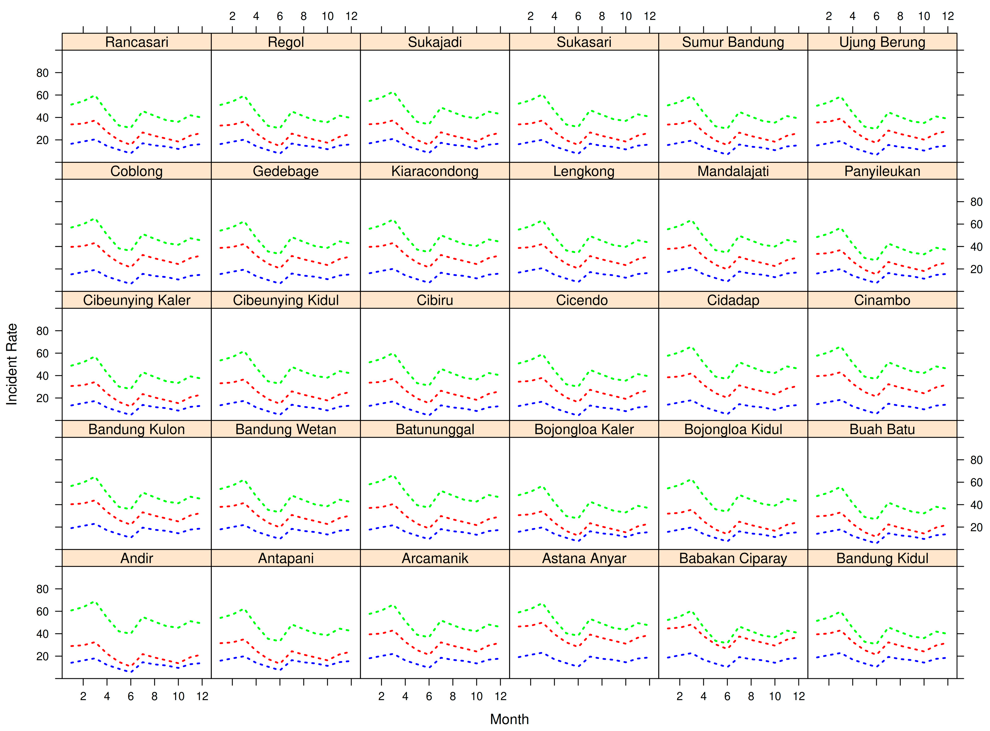
Figure 1 shows a quantile plot of the URTI data for each district of Bandung city. The three quantiles are displayed in different colors. Quantile 0.25 is blue, quantile 0.50 is red, and quantile 0.75 is green. Different patterns of three-level quantile functions are seen in all districts.
As can be seen in
Figure 1, there is variation in the distance between the quantile curves for each district. The largest gaps between quantiles 0.25 and 0.5 are found in Astana Anyar and Ciparay, and the largest gaps between quantiles 0.5 and 0.75 are found in Andir. The smallest distance between quantiles 0.25 and 0.50 was observed in Andir, and the smallest distance between quantiles 0.50 and 0.75 was found in Babakan Ciparay district.
Figure 1 shows that the 0.25 quantile curve has a similar trend in all districts and is less than 20, while the 0.50 quantile curve varies from district to district. On the other hand, at the quantile 0.75 we see much larger difference curves. Generally, quantile values are less than 80. The curves typically decrease through the middle of the year and then rise slightly to the end of the year.
3.3. Quantile Maps
The results related to spatial locations are shown through a quantile map. The map shows quantile values based on color grading. Small quantile values are represented by the light color (yellow), and high quantile values are represented by the dark colors (dark green).
The representative spatial maps of quantile URTI data of Bandung city are shown in
Figure 2 for February, May, August and November. Each map presents three quantile levels. The left is the 0.25 quantile, the middle is the 0.50 quantile, and the right is the 0.75 quantile.
Based on
Figure 2, the map patterns are similar over the months, whereas the gradation of the color tends to fade, both for quantiles 0.25, 0.50, and 0.75. However, the map patterns look different between quantile levels. For example, the eastern area shows relatively small values at the 0.25 and 0.50 quantiles, but fairly large values at the 0.75 quantile. The highest value is at quantile 0.75 present in February and the highest variations are in quantile 0.50.
3.4. Coefficient Plots of Time Variables
Figure 3 depicts coefficient plots of the time variables for the three quantile levels. The coefficient estimator (
) for quantile 0.25 is shown in (a)–(c), for quantile 0.50 in (d)–(f), and for quantile 0.75 in (g)–(i). In general, all estimates of slope 1 (a), (d), and (g) vary over time and decrease monotonically with various characteristics. Slope 2 estimators tend to decrease sharply from January to July, then level off or increase slightly until December. Moreover, the estimates of slope 3 (c), (f), and (i) increase monotonically with various patterns.
The greatest fluctuation was found at the 0.75 quantile especially for slope 2 (h). The estimators of coefficients of slope 1 () and slope 3 () have a negative effect on the response, while the coefficient of slope 2 () is positive.
3.5. Coefficient Maps of Spatial Variables
Figure 4,
Figure 5 and
Figure 6 show maps of the estimate of the space coefficients (
) for the three quantile levels. In general, the effect of spatial coefficients varies over spatial locations, but some variables have similar effects to others. It also contains intercept estimators (
) for the three quantile levels. The weaker effects are represented by lighter colors, while darker colors represent stronger effects. The estimated coefficients for slope 1 (
) and slope 2 (
) have negative effects, and positive effect for slope 3 (
).
As can be seen in
Figure 4, the varying coefficients appear in the slope 1 coefficients, although the variation of the effect looks very slight. Nonetheless, the slope 2 coefficient has relatively similar effects on each district, which also happen for slope 3. Almost no difference in effect appears for the intercept.
In
Figure 5, all estimated coefficients vary over spatial locations. There are five districts that have a strong negative effect on both slope 1 and slope 2. However, slope 3 shows a stronger effect, but few districts are weaker. Moreover, the estimates of the intercept have little difference in effects among districts.
Figure 6 shows two estimates of coefficients that vary over the districts. The varying coefficients appear clearly for slope 1, but there is slight variation in slope 2. Meanwhile, slope 3 shows no varying coefficient. Moreover, the intercept estimator has very little variation in the effects among districts. The two spatially varying coefficients, slope 1 and slope 2, have a negative effect, while slope 3 has a positive effect. In addition, the intercept has positive coefficient estimates.
4. Discussion
Varying coefficient models have been developed to incorporate multiple variables, with the ST-VCM being a specific model designed for longitudinal data that involves both space and time variations. In these models, the function of the covariates must be specified, but this can be difficult. To overcome this challenge, a nonparametric approach can be used as it is more flexible and does not require strict assumptions. Additionally, for data that has outliers or nonstandard conditional distributions, a robust model such as quantile regression can be used. This approach also provides more information about the distribution.
In this study, the incidence rate data of URTI in Bandung City were analyzed, which have a longitudinal structure and several covariates that are measured for each district, such as breast milk, malnutrition, and vitamin A. Other covariates were measured monthly for the entire city, such as temperature, rainfall, and humidity. The data structure lends itself well to the ST-VCM model, as the coefficients are not only varying over time but also over location.
According to the quantile plots (
Figure 1), different patterns for the three-level quantile functions were observed in all districts. Some areas exhibited a random structure, which required a flexible approach to estimate the curve. Variations in the distance between the quantile curves were observed for each district. This suggests that each sub-district has a different incidence rate every month. For example, the incidence rate in Andir in March was much higher than June, but it was also higher than the incidence rate in Ujung Berung at the same month. In general, the quantile maps (
Figure 2) showed the heterogeneity of quantiles among the districts, as seen in the color gradations of each quantile level map. The quantile maps showed a similar pattern from February to November, but the gradations tended to fade for all quantile levels. However, the pattern of quantile maps looked different, for example, in Cibiru and Panyileukan, which had relatively lighter quantile 0.25 and 0.50, but for quantile 0.75, it tended to be darker. The highest value was present in February for quantile 0.75, and the highest fluctuations were at quantile 0.50.
The time-varying coefficients were found to have estimators of temperature that varied over time and decreased monotonically with different characteristics. The rainfall estimators decrease drastically from January to July, then tend to be flat or increased slightly until December. Additionally, the estimators of humidity were found to increase monotonically with different patterns. The largest fluctuation was observed in quantile 0.75, particularly for rainfall. The estimators of the coefficients for temperature and humidity have a negative effect on the response, indicating that high temperature or humidity resulted in a low incidence rate of URTI. Conversely, the positive coefficient of rainfall indicates that high rainfall resulted in a high incidence rate of URTI.
The space-varying coefficients were found to have effects that varied over spatial locations, but some variables had similar effects for quantile 0.25. The varying coefficient appeared for the coefficient of breast milk, although the variation of the effect looked very slight. However, the coefficients of malnutrition had relatively similar effects for each district, and this also occurred for vitamin A. There were strong negative effects for both breast milk or malnutrition in Cicendo, Babakan Ciparay, Rancasari, Antapani, and Cibiru at quantile 0.50. Nevertheless, vitamin A showed more significant effects, but only a few districts had weaker effects. The analysis of the district-level data revealed that the coefficients for breast milk and malnutrition vary among districts for the quantile 0.75. The variation in the coefficient for breast milk is more pronounced compared to malnutrition. However, there was no variation in the coefficient for vitamin A. Additionally, the estimates for the intercept had minimal differences among districts. The coefficient for breast milk had a negative and strong impact on the incidence rate of URTI, indicating that higher levels of breast milk are associated with lower incidence rates. In contrast, the coefficient for malnutrition had a weak effect on the incidence rate. On the other hand, vitamin A had a positive coefficient, indicating that higher levels of vitamin A are associated with higher incidence rates. Furthermore, the intercepts had positive coefficient estimates.
5. Conclusions
In this study, a space-time varying coefficient model (ST-VCM) was applied to analyze longitudinal data in which the coefficients are allowed to vary as a smooth function of both space and time variables. The use of quantile regression within this model was also discussed, particularly in cases where the data contain outliers or non-standard conditional distributions. A nonparametric approach using P-splines was used to estimate the parameters of the ST-VCM. The ST-VCM was applied to incidence rate data of upper respiratory tract infections (URTI) in Bandung City, as these data exhibit a longitudinal structure and the covariates vary over both time and spatial location.
The study found that there are distinct patterns for three levels of quantiles in all districts, with the distance between the quantile curves varying from district to district. This indicates that each sub-district has a unique incidence rate for each level of quantile. Although the overall pattern of quantile curves is similar across all quantile levels, there are notable differences at the 0.50 and 0.75 quantile levels. The heterogeneity of quantiles among the districts can be observed through the color gradation of the quantile level maps. For example, the districts of Cibiru and Panyileukan have relatively lighter shades for the 0.25 and 0.50 quantiles but tend to be darker for the 0.75 quantile. The highest values for the 0.75 quantile were found in February, and the greatest fluctuations were observed at the 0.50 quantile.
The analysis also revealed that temperature and humidity have a negative effect on the incidence of upper respiratory tract infections (URTI), meaning that high temperatures or humidity lead to a lower incidence of URTI. In contrast, a positive coefficient was found for rainfall, indicating that high rainfall results in a higher incidence of URTI.
The study found that the space-varying coefficient for breast milk has a negative effect on incidence rate, indicating that higher levels of breast milk tend to correspond with lower incidence rates. In contrast, the coefficient for malnutrition had a very weak effect on incidence rate. Additionally, the coefficient for vitamin A was found to have a positive effect, meaning that higher levels of vitamin A tend to correspond with higher incidence rates. The intercepts were also found to have positive coefficient estimates. Furthermore, some of the coefficients were found to vary little, such as malnutrition at the 0.25 quantile and vitamin A at the 0.25 and 0.50 quantiles.
In general, the study concludes that the use of the space-time varying coefficient model (ST-VCM) on longitudinal data revealed differences in the effects between quantile levels for both space and time coefficients. The quantile curve created using the space and time coefficient estimates demonstrated robustness with respect to outliers, but some quantile curves still did not accurately describe the actual data pattern. This may be due to the simultaneous estimation procedure used to produce estimates that are relatively similar to one another.
In summary, the study found that the incidence rate of each sub-district in Bandung City varies based on three quantile levels, with the city as a whole displaying a heterogeneity of incidence rate. This variability can be associated to the different effects of temporal and spatial covariates. Thus, the recommendation for related institutions in making policies is to consider not only the district but also month, because each district has different effect characteristics for every month.
In this study, we investigated the separable space and time varying coefficients component of the Space-Time Varying Coefficient Model (ST-VCM). The ST-VCM also includes the simultaneous space-time effect, however, this aspect is not the focus of this paper. The simultaneous effect refers to the interaction between spatial location and time, whose importance is the use of a tensor product or Kronecker product in computation. This can lead to large matrices, particularly in the estimation of B-splines, making it an interesting topic for further research.


