Probability Analysis of a Stochastic Non-Autonomous SIQRC Model with Inference

Abstract

When an individual with confirmed or suspected COVID-19 is quarantined or isolated, the virus can linger for up to an hour in the air. We developed a mathematical model for COVID-19 by adding the point where a person becomes infectious and begins to show symptoms of COVID-19 after being exposed to an infected environment or the surrounding air. It was proven that the proposed stochastic COVID-19 model is biologically well-justifiable by showing the existence, uniqueness, and positivity of the solution. We also explored the model for a unique global solution and derived the necessary conditions for the persistence and extinction of the COVID-19 epidemic. For the persistence of the disease, we observed that ${\mathfrak{R}}_{\mathfrak{s}}^{\mathfrak{0}}>1$, and it was noticed that, for $R_s<1$, the COVID-19 infection will tend to eliminate itself from the population. Supplementary graphs representing the solutions of the model were produced to justify the obtained results based on the analysis. This study has the potential to establish a strong theoretical basis for the understanding of infectious diseases that re-emerge frequently. Our work was also intended to provide general techniques for developing the Lyapunov functions that will help the readers explore the stationary distribution of stochastic models having perturbations of the nonlinear type in particular.

1. Introduction

The pathogen SARS-CoV-2 is responsible for the spread of COVID-19, and it is an infectious illness characterized by its genetic material enveloped by a lipid and protein outer layer. The membrane consists of structures (spike proteins) that allow the virus to associate with human tissues throughout infection. Due to the numerous factors that influence the efficiency of environmental transfer, the incidence rate of SARS-CoV-2 fomite transfer is reported to be low when contrasted with direct interaction, airborne, or droplet transmission [1,2]. When an individual with confirmed or suspected COVID-19 is quarantined or isolated, the virus can linger for up to an hour in the air. The time for which a virus continues to remain suspended and contagious is determined by a variety of factors, which include viral load in airborne droplets or tiny particles, surfaces and air disturbances, temperature, airflow, and humidity [3,4,5]. Individuals can become infected with severe acute respiratory disease by contacting surfaces. Based on available epidemiological studies and ecological transmission factors, the risk of severe acute respiratory syndrome spreading through surface transmission is believed to be moderate and not the typical route of transmission. Individuals become infected with SARS-CoV-2 primarily through contact with the virus-carrying droplets in the air [6,7,8].

Numerous mathematical models for showing the transmission behavior of COVID-19 have been investigated, and the readers are suggested to see [9,10,11,12]. Plenty of COVID-19’s mathematical problems have been built assuming the natural and discrete pattern of the problems, with some constraints to depict the true evaluation of the underlying epidemics. Contemporary calculus provides a valuable tool for providing patterns and extra outcomes of the diseases that are required for understanding the hidden insights of mathematical models, in particular in the planning and control of infectious diseases. Equations involving the non-integer-order derivatives have memory appropriateness, and such equations provide an excellent situation for depicting the real scenario of infectious diseases. Arbitrary-order differential equations are often found to be useful in many situations, as they also possess interesting properties.

It is strongly advised to use mathematical modeling tools when investigating the spreading mechanism and controlling epidemics [12,13,14,15,16], and one can notice that tools of fractional differential equations are applicable in various branches of science [17,18,19]. In depicting the evolutionary history of infectious disease, differential equations can find a balance between biological rationality and the power of their connection with the data. The COVID-19 models developed thus far, from epidemics to population densities, have shown a diverse range of patterns. Climate sources of noise are consistently the most-essential components of physical mechanisms and biological systems. It is observed that, like other diseases, the variations in the pattern has a considerable impact on the spread and emergence of COVID-19; for instance, see [20]. Due to the unpredictability in the interactions and other known features of the human population, the emergence of epidemics, its growth, and its spread in the population are also unpredictable. It is well justified and proven that the environmental variations influence the state of the infectious disease, and up to great extent, these variations makes the epidemic unpredictable.

The distribution and persistence of infectious diseases are significantly influenced by the alterations of environmental factors. Epidemiological studies consider the randomness of variables and of crucial parameters because it reflects the actual dynamic nature of an infection. Although the variations are random in nature, they must be strongly autocorrelated. Furthermore, the perturbations can be determined analytically by using the related problem’s density function of probabilities [21,22,23,24]. There are two fundamental approaches for formulating epidemic models: the deterministic and the stochastic approach. When it comes to modeling biological phenomena, stochastic models are preferred over deterministic models because they have the potential to provide a higher level of realism than deterministic systems [24,25,26,27]. SDEs can be used to generate a distribution of the expected outcome(s), such as the density of the infective class at a time t. In addition, a stochastic model can generate more valuable output results compared to a deterministic model when simulated multiple times, unlike a deterministic model that produces a single result regardless of the number of experiments conducted. Several deterministic epidemiological studies have been presented to explain the dynamics of the highly contagious COVID-19; for instance, see [28,29].

In this paper, we suggest an epidemic model based on a stochastic approach to modeling to try to explain the dynamic behavior of the COVID-19 epidemic, especially its long-term behavior. The entire human population was divided into four distinct compartments, and one class was reserved for the virus that spreads COVID-19. These disjoint compartments were: the susceptibles, infectives, quarantined, recovered, and the virus compartment, which persists in the air, on human bodies, and on surfaces, and their sizes are denoted by $\mathbb{S}\left(t\right)$, $\mathbb{I}\left(t\right)$, $\mathbb{Q}\left(t\right)$, $\mathbb{R}\left(t\right)$, and $\mathbb{C}\left(t\right)$. These compartments are connected with one another according to the features of the disease, and ecological noise sources were taken into account. More specifically, we introduced the time interval between when a person becomes contagious and when he/she begins to exhibit COVID-19 signs and symptoms.

The paper is structured as follows. In Section 2, we formulate the COVID-19 model based on the underlying assumptions. Section 3 proves the equilibria of the deterministic model and its corresponding basic reproduction number. Section 4 discusses the existence of the one and only positive global solution. In Section 5 and Section 6, we develop the necessary and sufficient conditions for the persistence and extinction of the disease. In Section 7, the theoretical results are experimentally verified and graphically presented. Section 8 contains a detailed analysis of the study, and the conclusion and suggestions for further research are presented.

2. Model’s Formulation

We developed a mathematical model for COVID-19 by adding the time period in which an individual is infected and the development of symptoms. Further, the study included some environmental fluctuations such as the surfaces and air, humidity, temperature, and ventilation. The proposed model is a susceptible–infectious–quarantined–recovered model in the human population, and further, the model assumes the density of virus that causes COVID-19. Each compartment’s size in the human population is mathematically represented as $\mathbb{S}\left(t\right)$, $\mathbb{I}\left(t\right)$, $\mathbb{Q}\left(t\right)$, and $\mathbb{R}\left(t\right)$ at any time t, and it shows the amount of the susceptible, infected, quarantined, and recovered populations. In addition, the symbol $\mathbb{C}\left(t\right)$ stands for the disturbance of the surfaces and air, humidity, temperature, and ventilation. The recruitment into the population is described by the positive constant $\Pi$, and it will be added into the susceptible compartment. The natural removal rate from the human population is denoted by $\mu$, and it is constant for all the compartments. The vulnerable population will catch COVID-19 at a rate of $\beta \mathbb{C}\left(t\right)$. The term $\beta$ assumes positive real values, and biologically, it shows the rate of ingestion due to the COVID-19 virus in the disturbances of the surfaces and air, humidity, ventilation, etc. After completing the infectious period, an individual may recover, and after the recovery, he or she may lose immunity at a rate of $\omega$. Thus, $\omega R\left(t\right)$ is the number of recovered people that will move to the vulnerable class in a unit of time. Infectious persons can agree to be quarantined for a certain duration of time. Throughout that time, individuals are detached from the population and given appropriate medicines at a low frequency $\delta$. The quarantined people will tend to recover at a rate $\epsilon$, and thus, $\epsilon Q\left(t\right)$ individuals will move to the recovered compartment. The death rates associated with COVID-19 in the infected and quarantined classes are, respectively, ${\alpha }_1$ and ${\alpha }_2$. When an individual becomes infected with the COVID-19 virus, he or she will contribute to the virus concentration at the rate $\eta$ within a unit of time. At the same time, the virus density level could decrease at a rate d, which usually occurs due to the mortality of the virus. Besides this, we imposed the following assumptions while formulating the model:

A₁: 

It was assumed that $\mu ,{\Lambda },\beta ,{\eta }_1,\kappa ,d$, and ${\eta }_2$ are greater than zero, whereas the parameters $\delta ,\omega ,\epsilon ,{\alpha }_1$, and ${\alpha }_2$ are nonnegative.

A₂: 

Within a given time period, the value of the parameter c represents the average size of the contacts.

A₃: 

Each compartmental unit ($\mathbb{S}\mathbb{I}\mathbb{Q}$ and $\mathbb{R}$) in the human population has an equal chance of moving to another group. Similarly, the virus can move from the infected human compartments to the virus concentration $\mathbb{C}$ class. In other words, the random variable determines the probabilities of progressing among groups, and the predictive time being spent in a group can be calculated by taking into account the inverse of that component in a probability function.

A₄: 

Assume that the population is closed and remains constant over time. This means, the model represents the spread of the disease within a confined population.

A₅: 

If the population is flexible, an additional shift coefficient must be included in the model to take into consideration discharges, the recruitment of new susceptibles, and deaths. To preserve the endemic situation in a community, one needs to consider a population where inflows and outflows are assumed.

A₆: 

Persons in the R class already have completed their intervention, are immune, and thus, resistant to COVID-19. We presumed that almost no immune person died as a result of COVID-19. In this light, it is reasonable to assume that both vulnerable and immune people die at the natural mortality rate $\mu$. Our belief is that only individuals who are contagious, untreated, and displaying symptoms or who are undergoing treatment are susceptible to fatal outcomes from the disease.

These hypotheses were transformed into the mathematical equations shown below:

$$\begin{array}{c}\hfill \begin{array}{cc}\hfill \frac{d\mathbb{S}}{dt}& =\Pi -\frac{\beta \mathbb{C}\left(t\right)\mathbb{S}\left(t\right)}{\mathbb{N}\left(t\right)}+\omega \mathbb{R}\left(t\right)-\mu \mathbb{S}\left(t\right),\hfill \\ \hfill \frac{d\mathbb{I}}{dt}& =\frac{\beta \mathbb{C}\left(t\right)\mathbb{S}\left(t\right)}{\mathbb{N}\left(t\right)}-({\alpha }_1+\mu +\delta )\mathbb{I}\left(t\right),\hfill \\ \hfill \frac{d\mathbb{Q}}{dt}& =\delta \mathbb{I}\left(t\right)-({\alpha }_2+\mu +\epsilon )\mathbb{Q}\left(t\right),\hfill \\ \hfill \frac{d\mathbb{R}}{dt}& =\epsilon \mathbb{Q}\left(t\right)-(\mu +\omega )\mathbb{R}\left(t\right),\hfill \\ \hfill \frac{d\mathbb{C}}{dt}& =\eta \mathbb{I}\left(t\right)-d\mathbb{C}\left(t\right).\hfill \end{array}\end{array}$$

(1)

We developed a flow diagram for System (1), which is shown in Figure 1.

In order to include the environmental fluctuations in Model (1), we shall consider the standard Brownian motions $W_i\left(t\right)$ for $i=1,2,3,4,5$ having the property of $W_i\left(0\right)=0$. Associated with these motions, we have the positive real numbers ${\xi }_1,{\xi }_2,{\xi }_3,{\xi }_4,{\xi }_5$, which physically describes the respective intensities of the noises. With these notions, we have the stochastic model of the form:

$$\begin{array}{c}\hfill \begin{array}{cc}\hfill d\mathbb{S}& =\left[\Pi -\frac{\beta \mathbb{C}\left(t\right)\mathbb{S}\left(t\right)}{\mathbb{N}\left(t\right)}+\omega \mathbb{R}\left(t\right)-\mu \mathbb{S}\left(t\right)\right]dt+{\xi }_1\mathbb{S}\left(t\right)d{\mathbb{W}}_1\left(t\right),\hfill \\ \hfill d\mathbb{I}& =\left[\frac{\beta \mathbb{C}\left(t\right)\mathbb{S}\left(t\right)}{\mathbb{N}\left(t\right)}-({\alpha }_1+\mu +\delta )\mathbb{I}\left(t\right)\right]dt+{\xi }_2\mathbb{I}\left(t\right)d{\mathbb{W}}_2\left(t\right),\hfill \\ \hfill d\mathbb{Q}& =\left[\delta \mathbb{I}\left(t\right)-({\alpha }_2+\mu +\epsilon )\mathbb{Q}\left(t\right)\right]dt+{\xi }_3\mathbb{Q}\left(t\right)d{\mathbb{W}}_3\left(t\right),\hfill \\ \hfill d\mathbb{R}& =\left[\epsilon \mathbb{Q}\left(t\right)-(\mu +\omega )\mathbb{R}\left(t\right)\right]dt+{\xi }_4\mathbb{R}\left(t\right)d{\mathbb{W}}_4\left(t\right),\hfill \\ \hfill d\mathbb{C}& =\left[\eta \mathbb{I}\left(t\right)-d\mathbb{C}\left(t\right)\right]dt+{\gamma }_5{\mathbb{B}}_1\left(t\right)d{\mathbb{W}}_5\left(t\right),\hfill \end{array}\end{array}$$

(2)

A flow diagram for System (2) was created and is presented in Figure 2.

Keeping in view Model (2), we particularly intended to address the following claims:

Q₁: 

The stochastic noises affect the dynamics of COVID-19 to a great extent.

Q₂: 

The contaminated surfaces and air, humidity, temperature, and ventilation play a significant role in the spreading of the disease.

Q₃: 

A criterion exists that guarantees the eradication of the infection.

Q₄: 

By describing the dynamics of the disease via the proposed model, the disease may also persist in the population when the parameters obey some pre-defined rule.

3. Deterministic Model Analysis

In this section, our aim was to demonstrate the validity of Model (1) by proving that the system’s solution remains nonnegative for any set of nonnegative initial data. Furthermore, we provide the expression for endemic and disease-free equilibria, as well as determined the threshold parameter ($R_0$), called the basic reproduction number. After linearizing the model, we can obtain several significant results to test the stability of the equilibrium points. For future use, we present the following notations:

$$\begin{array}{cc}\hfill a_1& =\delta +{\alpha }_1+\mu ,\hfill \\ \hfill a_2& =\epsilon +{\alpha }_2+\mu ,\hfill \\ \hfill a_3& =\omega +\mu ,\hfill \\ \hfill {\rho }_1& =\Pi \eta a_2{a}_3+d(a_1{a}_2{a}_3-\delta \epsilon ),\hfill \\ \hfill \overline{D}& =a_1{a}_2{a}_3\mu +\beta (a_1{a}_2{a}_3-\delta \epsilon \omega ),\hfill \\ \hfill A& =a_1{a}_2{a}_3,\hfill \\ \hfill \tilde{A}& =a_1{a}_2{a}_3-\delta \epsilon \omega .\hfill \end{array}$$

(3)

Equilibria and the Term $R_0$

In order to find the equilibria of the model, we considered the time-absent problem. That is, we assumed those values of the state variables for which the system exhibits no change with respect to time. In the present case, our state variables satisfy

$$\frac{d\mathbb{S}}{dt}=\frac{d\mathbb{I}}{dt}=\frac{d\mathbb{Q}}{dt}=\frac{d\mathbb{R}}{dt}=\frac{d\mathbb{C}}{dt}=0,$$

(4)

and solving this set of equations yields the constant function(s). It is worth mentioning that the delay terms have no effect on these constant solutions; therefore, the proposed model has a disease-free fixed point similar to [30] and is given by

$${\mathbb{E}}^0=\left({\mathbb{S}}^0,{\mathbb{I}}^0,{\mathbb{Q}}^0,{\mathbb{R}}^0,{\mathbb{C}}^0\right)=\left(\frac{\Pi }{\mu },0,0,0,0\right).$$

(5)

Following the same process, we have an expression for the threshold parameter as

$$R_0=\frac{\beta \Pi \eta }{\mu d(\delta +{\alpha }_1+\mu )}.$$

(6)

Moreover, when $R_0>1$, the model has an endemic fixed point, which is given by

$$E^{*}=\left({\mathbb{S}}^{*},{\mathbb{I}}^{*},{\mathbb{Q}}^{*},{\mathbb{R}}^{*},{\mathbb{C}}^{*}\right),$$

(7)

where

$$\begin{array}{cc}\hfill {\mathbb{S}}^{*}& =\frac{a_1\rho }{{\eta }_1{\eta }_2\overline{D}},\hfill \\ \hfill {\mathbb{I}}^{*}& =\frac{\beta \Pi a_2{a}_3\left(R_0-1\right)}{R_0\overline{D}},\hfill \\ \hfill {\mathbb{Q}}^{*}& =\frac{\beta \Pi a_3\delta \left(R_0-1\right)}{R_0\overline{D}},\hfill \\ \hfill {\mathbb{R}}^{*}& =\frac{\beta \Pi \delta \epsilon \left(R_0-1\right)}{R_0\overline{D}},\hfill \\ \hfill {\mathbb{C}}^{*}& =\frac{\beta \Pi \eta a_2{a}_3\left(R_0-1\right)}{R_0\overline{D}d}\hfill \end{array}$$

(8)

4. Stochastic Model Analysis

This section investigates the uniqueness and existence of the solutions, the asymptotic behavioral patterns, the extinction situations, and the stationary distribution of an ergodic nature in the stochastic system.

Positive Global Solution of the Model

The initial and critical inquiry when examining the dynamic characteristics of a model is to check whether a global solution of the proposed system is possible or not. Furthermore, for a model that describes the dynamics of a population, the appearance of its solution’s values is of significant concern. In this section, we established that the solution of Model (2) is global and nonnegative. It is well recognized that, regardless of the specified initial condition, the co-efficient of a stochastic equation must satisfy the linearly increasing condition, as well as the local Lipschitz characteristic in order to have a unique solution (that is, no outburst in a specified interval).

Theorem 1.

Model (2) will have a unique solution $\left(\mathbb{S}\right(t),\mathbb{I}(t),\mathbb{Q}(t),\mathbb{R}(t),\mathbb{C}(t\left)\right)$ subject to any initial values of the state variables from ${\mathbb{R}}_{+}^5$ and $t\ge 0$. In addition, this solution will remain in ${\mathbb{R}}_{+}^5$ with probability one.

Proof. 

By referencing the fact that $(\mathbb{S}\left(0\right),\mathbb{I}\left(0\right),\mathbb{Q}\left(0\right),\mathbb{R}\left(0\right),\mathbb{C}\left(0\right))\in {\mathbb{R}}_{+}^5$ and from the locally Lipschitzness of the terms, the underlying problem has a unique local solution $(\mathbb{S},{\mathbb{V}}_1,{\mathbb{V}}_2,\mathbb{E},\mathbb{I},\mathbb{R})$ over the interval $[0,{\tau }_e)$. Here, ${\tau }_e\ge 0$ represents the physical expulsion time, and for a detail explanation, we recommend the readers see [31,32]. The subsequent step is to prove that this solution is indeed global, which requires demonstrating that a.s. ${\tau }_e=\infty$. Initially, we must show that the solution does not become unbounded within a finite time. To do so, let us choose a sufficiently large positive real number $k_0$ such that the problem’s solution lies in the interval $[\frac{1}{k_0},k_0]$. We define the following term and assumed that $k\ge k_0$:

$$\begin{array}{c}\hfill {\tau }_k=inf\{t\in [0,{\tau }_e):\frac{1}{k}\ge min\{\mathbb{S}\left(t\right),\mathbb{I}\left(t\right),\mathbb{Q}\left(t\right),\mathbb{R}\left(t\right),\mathbb{C}\left(t\right)\}\mathrm{or}\\ \hfill k\le max\left\{\mathbb{S}\right(t),\mathbb{I}(t),\mathbb{Q}(t),\mathbb{R}(t),\mathbb{B}(t),\mathbb{C}(t\left)\right\}.\end{array}$$

(9)

Suppose $inf\varnothing =\infty$ whenever ∅ is an empty set. It is easy to show that ${\tau }_k$ increases if we let the term k increase. By letting k tend to ∞ and, hence, ${\tau }_k$ approach ${\tau }_{\infty }$, it follows that ${\tau }_e\to \infty$. Therefore, demonstrating that ${\tau }_{\infty }$ approaches infinity a.s. ensures that ${\tau }_e$ also approaches infinity. Establishing all these facts guarantees that $(\mathbb{S}\left(t\right),\mathbb{I}\left(t\right),\mathbb{Q}\left(t\right),\mathbb{R}\left(t\right),\mathbb{C}\left(t\right))\in {\mathbb{R}}_{+}^5$ for any time $t\ge 0$. Let us consider the case where ${\tau }_e\ne \infty$. In that scenario, there should exist a nonnegative real number T and $ϵ\in (0,1)$ such that:

$$ϵ<P\{{\tau }_{\infty }\le T\}.$$

(10)

Hence, for $k_0\le k_1$, we have

$$P\{T\ge {\tau }_k\}\ge ϵ,\forall k_1\le k.$$

Before moving further, consider the following Lyapunov function:

$$\begin{array}{c}\hfill \begin{array}{cc}\hfill \mathbb{V}& =(\mathbb{S}-1-\log \mathbb{S})+(I-log\mathbb{I}-1)+(\mathbb{Q}-\log \mathbb{Q}-1)+(\mathbb{R}-\log \mathbb{R}-1)\hfill \\ & +(\mathbb{C}-\log \mathbb{C}-1),\hfill \end{array}\end{array}$$

(11)

By considering the well-known $It\widehat{o}$ formula, letting $k_0\le k$ and assume a very large positive value of T, Relation (11) becomes

$$\begin{array}{c}\hfill \begin{array}{cc}\hfill d\mathbb{V}(\mathbb{S},\mathbb{I},\mathbb{Q},\mathbb{R},\mathbb{C})& =L\mathbb{V}(\mathbb{S},\mathbb{I},\mathbb{Q},\mathbb{R},\mathbb{C})dt+{\xi }_1(\mathbb{S}-1)d{\mathbb{W}}_1\left(t\right)+{\xi }_2(\mathbb{I}-1)d{\mathbb{W}}_2\left(t\right)\hfill \\ & +{\xi }_3(\mathbb{Q}-1)d{\mathbb{W}}_3\left(t\right)+{\xi }_3(\mathbb{R}-1)d{\mathbb{W}}_4\left(t\right)+{\xi }_5(\mathbb{C}-1)d{\mathbb{W}}_5\left(t\right).\hfill \end{array}\end{array}$$

(12)

In Equation (12), the $L\mathbb{V}$ operator is from ${\mathbb{R}}_{+}^5\to {\mathbb{R}}_{+}$ and is given by

$$\begin{array}{cc}\hfill L\mathbb{V}& =\left(1-\frac{1}{\mathbb{S}}\right)\left(\Pi -\frac{\beta \mathbb{C}\mathbb{S}}{\mathbb{N}}+\omega \mathbb{R}-\mu \mathbb{S}\right)+\frac{1}{2}{\xi }_1{}^2\hfill \\ \hfill & +\left(1+\frac{1}{\mathbb{I}}\right)\left(\frac{\beta \mathbb{C}\mathbb{S}}{\mathbb{N}}-({\alpha }_1+\mu +\delta )\mathbb{I}\right)+\frac{1}{2}{\xi }_2{}^2\hfill \\ \hfill & +\left(1-\frac{1}{\mathbb{Q}}\right)\left(\delta \mathbb{I}-({\alpha }_2+\mu +\epsilon )\mathbb{Q}\right)+\frac{1}{2}{\xi }_3{}^2+\left(1-\frac{1}{\mathbb{R}}\right)\left(\epsilon \mathbb{Q}-(\mu +\omega )\mathbb{R}\right)+\frac{1}{2}{\xi }_4{}^2\hfill \\ \hfill & +\left(1-\frac{1}{\mathbb{C}}\right)\left(\eta \mathbb{I}-d\mathbb{C}\right)+\frac{1}{2}{\xi }_5{}^2,\hfill \\ \hfill & =\Pi -\frac{\beta \mathbb{C}\mathbb{S}}{\mathbb{N}}+\omega \mathbb{R}-\mu \mathbb{S}-\frac{\Pi }{\mathbb{S}}+\frac{\beta {\mathbb{B}}_2}{\mathbb{N}}-\frac{\omega \mathbb{R}}{\mathbb{S}}+\mu +\frac{\beta \mathbb{C}\mathbb{S}}{\mathbb{N}}-({\alpha }_1+\mu +\delta )\mathbb{I}\hfill \\ \hfill & -\frac{\beta \mathbb{C}\mathbb{S}}{\mathbb{N}\mathbb{I}}+({\alpha }_1+\mu +\delta )+\delta \mathbb{I}-({\alpha }_2+\mu +\epsilon )\mathbb{Q}-\frac{\delta }{\mathbb{Q}}-({\alpha }_2+\mu +\epsilon )\hfill \\ \hfill & +\epsilon \mathbb{Q}-(\mu +\omega )\mathbb{R}-\frac{\epsilon \mathbb{Q}}{\mathbb{R}}-(\mu +\omega )+\eta \mathbb{I}-d\mathbb{C}-\frac{\eta \mathbb{I}}{\mathbb{C}}+d\hfill \\ \hfill & +\frac{{\xi }_1{}^2+{\xi }_2{}^2+{\xi }_3{}^2+{\xi }_4{}^2+{\xi }_5{}^2}{2},\hfill \\ \hfill & \le \Pi +\mu +({\alpha }_1+\mu +\delta )+({\alpha }_2+\mu +\epsilon )+(\mu +\omega )+\eta \mathbb{I}+d\hfill \\ \hfill & +\frac{{\xi }_1{}^2+{\xi }_2{}^2+{\xi }_3{}^2+{\xi }_4{}^2+{\xi }_5{}^2}{2},\hfill \end{array}$$

(13)

Furthermore, we know that $\mathbb{S}+\mathbb{I}+\mathbb{Q}+\mathbb{R}\le 1$; thus,

$$\begin{array}{cc}\hfill L\mathbb{V}& \le \Pi +4\mu +{\alpha }_1\delta +{\alpha }_2+\epsilon +\omega +\eta +d+\frac{{\xi }_1{}^2+{\xi }_2{}^2+{\xi }_3{}^2+{\xi }_4{}^2+{\xi }_5{}^2}{2}=K.\hfill \end{array}$$

(14)

The remainder of the proof is similar to that of Theorem 2.1 in [27]. Therefore, it is easy for the reader to follow the outcome, and as a result, it is omitted. □

5. Extinction

When modeling the dynamical aspects of an epidemic disease, it is essential to examine the conditions under which the epidemic will be eliminated or disappear from the population. In this section, we illustrate that, for sufficient intensity of white noise, solution of System (2) will surely approach zero. Let us define the following:

$$\begin{array}{c}\hfill {\displaystyle \langle \mathbb{B}\left(t\right)\rangle =\frac{1}{t}{\int }_0^t\mathbb{B}\left(s\right)ds.}\end{array}$$

Lemma 1

([33,34]). (Strong law) Let ${\left\{\mathbb{Z}\right\}}_{0\le t}=\mathbb{Z}$ be continuous and real-valued along with local martingale, which approaches zero as $t\to 0$, then

$$\begin{array}{cc}\hfill & \underset{t\to \infty }{lim}{〈\mathbb{Z},\mathbb{Z}〉}_t=\infty ,a.s.,\Rightarrow \underset{t\to \infty }{lim}\frac{{\mathbb{Z}}_t}{{〈\mathbb{Z},\mathbb{Z}〉}_t}=0,a.s.\hfill \\ \hfill & \underset{t\to \infty }{lim}sup\frac{{〈\mathbb{Z},\mathbb{Z}〉}_t}{t}<0,a.s.,\Rightarrow \underset{t\to \infty }{lim}\frac{{\mathbb{Z}}_t}{t}=0,a.s.\hfill \end{array}$$

(15)

Lemma 2.

Consider a solution of System (2) of the form $(\mathbb{S},\mathbb{I},\mathbb{Q},\mathbb{R},\mathbb{C})$ subject to the initial conditions $\left(\mathbb{S}\right(0),\mathbb{I}(0),\mathbb{Q}(0),\mathbb{R}(0),\mathbb{C}(0\left)\right)$ in the space ${\mathbb{R}}_{+}^5$. Then,

$$\begin{array}{cc}\hfill \underset{t\to \infty }{lim\; sup}\frac{ln\mathbb{S}\left(t\right)}{t}& =0,\underset{t\to \infty }{lim\; sup}\frac{ln\mathbb{I}\left(t\right)}{t}=0,\underset{t\to \infty }{lim\; sup}\frac{ln\mathbb{Q}\left(t\right)}{t}=0,\hfill \\ \hfill \underset{t\to \infty }{lim\; sup}\frac{ln\mathbb{R}\left(t\right)}{t}& =0,\underset{t\to \infty }{lim\; sup}\frac{ln\mathbb{C}\left(t\right)}{t}=0,a.s.\hfill \end{array}$$

(16)

Furthermore, if $\mu >\frac{{\xi }_1^2\vee {\xi }_2^2\vee {\xi }_3^2\vee {\xi }_4^2}{2}$ and $d>\frac{{\xi }_5^2}{2}$, then

$$\begin{array}{cc}\hfill \underset{t\to \infty }{lim}\frac{{\int }_0^t\mathbb{S}\left(s\right)d{\mathbb{W}}_1\left(s\right)}{t}& =0,\underset{t\to \infty }{lim}\frac{{\int }_0^t\mathbb{I}\left(u\right)d{\mathbb{W}}_2\left(u\right)}{t}=0,\underset{t\to \infty }{lim}\frac{{\int }_0^t\mathbb{Q}\left(u\right)d{\mathbb{W}}_3\left(u\right)}{t}=0,\hfill \\ \hfill \underset{t\to \infty }{lim}\frac{{\int }_0^t\mathbb{R}\left(s\right)d{\mathbb{W}}_4\left(s\right)}{t}& =0,\underset{t\to \infty }{lim}\frac{{\int }_0^t\mathbb{C}\left(s\right)d{\mathbb{W}}_5\left(s\right)}{t}=0,a.s.\hfill \end{array}$$

(17)

Then, the solution of (2) is

$$\begin{array}{cc}\hfill \underset{t\to \infty }{lim\; sup}\mathbb{S}\left(t\right)& = \frac{\Pi }{\mu },\hfill \\ \hfill \underset{t\to \infty }{lim\; sup}\mathbb{I}\left(t\right)& =0,\hfill \\ \hfill \underset{t\to \infty }{lim\; sup}\mathbb{Q}\left(t\right)& =0,\hfill \\ \hfill \underset{t\to \infty }{lim\; sup}\mathbb{R}\left(t\right)& =0,\hfill \\ \hfill \underset{t\to \infty }{lim\; sup}\mathbb{C}\left(t\right)& =0,a.s.\hfill \end{array}$$

(18)

To prove Lemma 2, we followed an almost similar procedure as performed in the proof of Lemmas 2.1 and 2.2 carried out in the work of Zhao [33], and therefore, the proof is left for the readers.

In order to formulate the extinction theory for System (2), we begin by defining the threshold value ${\mathbb{R}}_s$ for the stochastic model, given by:

$$\begin{array}{ccc}\hfill R_s& =& \frac{\beta \eta }{d\left({\alpha }_1+\mu +\delta +\frac{{\xi }_2^2}{2}\right)}\hfill \end{array}$$

Theorem 2.

Consider a solution of System (2) of the form $(\mathbb{S},\mathbb{I},\mathbb{Q},\mathbb{R},\mathbb{C})$ subject to the initial state of the population $(\mathbb{S},\mathbb{I},\mathbb{Q},\mathbb{R},\mathbb{C})\left(0\right)$ in the space ${\mathbb{R}}_{+}^5$. Then, for $1>R_s$, the corresponding solution of Model (2) will satisfy the following:

$$\begin{array}{cc}\hfill & \underset{t\to \infty }{lim}〈\mathbb{S}\left(t\right)〉= \frac{\Pi }{\mu },a.s,\hfill \\ \hfill & \underset{t\to \infty }{lim}〈\mathbb{I}\left(t\right)〉=0,a.s,\hfill \\ \hfill & \underset{t\to \infty }{lim}〈\mathbb{Q}\left(t\right)〉=0,a.s,\hfill \\ \hfill & \underset{t\to \infty }{lim}〈\mathbb{R}\left(t\right)〉=0,a.s,\hfill \\ \hfill & \underset{t\to \infty }{lim}〈\mathbb{C}\left(t\right)〉=0,a.s,\hfill \end{array}$$

(19)

and this indicates that COVID-19 will surely be eliminated from the community.

Proof. 

The following relations could be easily obtained if one integrates System (2) in the interval $[0,t]$:

$$\begin{array}{c}\hfill \begin{array}{cc}& \frac{1}{t}(\mathbb{S}\left(t\right)-\mathbb{S}\left(0\right))=\Pi -\frac{\beta 〈\mathbb{C}〉〈\mathbb{S}〉}{〈\mathbb{N}〉}+\omega 〈\mathbb{R}〉-\mu 〈\mathbb{S}〉+\frac{{\xi }_1{\int }_0^t\mathbb{S}\left(r\right)d{\mathbb{W}}_1\left(r\right)}{t},\hfill \\ & \frac{1}{t}(\mathbb{I}\left(t\right)-\mathbb{I}\left(0\right))=\frac{\beta 〈\mathbb{C}〉〈\mathbb{S}〉}{〈\mathbb{N}〉}-({\alpha }_1+\mu +\delta )〈\mathbb{I}〉+\frac{{\xi }_2{\int }_0^t\mathbb{I}\left(r\right){\mathbb{W}}_2\left(r\right)}{t},\hfill \\ & \frac{1}{t}(\mathbb{Q}\left(t\right)-\mathbb{Q}\left(0\right))=\delta 〈\mathbb{I}〉-({\alpha }_2+\mu +\epsilon )〈\mathbb{Q}〉+\frac{{\xi }_3{\int }_0^t\mathbb{Q}\left(r\right)d{\mathbb{W}}_3\left(r\right)}{t},\hfill \\ & \frac{1}{t}(\mathbb{R}\left(t\right)-\mathbb{R}\left(0\right))=\epsilon 〈\mathbb{Q}〉-(\mu +\omega )〈\mathbb{R}〉+\frac{{\xi }_4{\int }_0^t\mathbb{R}\left(r\right)d{\mathbb{W}}_4\left(r\right)}{t},\hfill \\ & \frac{1}{t}(\mathbb{C}\left(t\right)-\mathbb{C}\left(0\right))=\eta 〈\mathbb{I}〉-d〈\mathbb{C}〉+\frac{{\xi }_5{\int }_0^t\mathbb{C}\left(r\right)d{\mathbb{W}}_5\left(r\right)}{t},\hfill \end{array}\end{array}$$

(20)

The last equation of Model (20) gives the following:

$$\begin{array}{c}\hfill \begin{array}{cc}\hfill 〈\mathbb{C}〉& =\frac{\eta }{d}〈\mathbb{I}〉-\frac{1}{d}\left(\frac{\mathbb{C}\left(t\right)-\mathbb{C}\left(0\right)}{t}\right)+\frac{{\xi }_5}{d}\left(\frac{{\int }_0^t\mathbb{C}\left(r\right)d{\mathbb{W}}_5\left(r\right)}{t}\right),\hfill \\ & =\frac{\eta }{d}〈\mathbb{I}〉+{\mathbb{Z}}_1\left(t\right),\hfill \end{array}\end{array}$$

(21)

where

$${\mathbb{Z}}_1\left(t\right)=-\frac{1}{d}\left(\frac{\mathbb{C}\left(t\right)-\mathbb{C}\left(0\right)}{t}\right)+\frac{{\xi }_5}{d}\left(\frac{{\int }_0^t\mathbb{W}\left(r\right)d{\mathbb{W}}_5\left(r\right)}{t}\right).$$

(22)

The $It\widehat{o}$ formula and the $2nd$ equation of system (2) will give us

$$\begin{array}{c}\hfill \begin{array}{cc}\hfill dlog\mathbb{I}& =\left[\frac{\beta \mathbb{C}\mathbb{S}}{\mathbb{I}\mathbb{N}}-({\alpha }_1+\mu +\delta )-\frac{{\xi }_2^2}{2}\right]dt+{\xi }_{2}d{\mathbb{W}}_2\left(t\right),\hfill \\ & \le \left[\frac{\beta \mathbb{C}}{\mathbb{I}}-({\alpha }_1+\mu +\delta +\frac{{\xi }_2^2}{2})\right]dt+{\xi }_{2}d{\mathbb{W}}_2\left(t\right).\hfill \end{array}\end{array}$$

(23)

Taking the integral of Expression (23) into the interval $[0,t]$ and multiplying the resultant relation by $t^{-1}$, we have

$$\begin{array}{c}\hfill \begin{array}{cc}\hfill \frac{log\mathbb{I}-\log \mathbb{I}\left(0\right)}{t}& \le \left[\frac{\beta 〈\mathbb{C}〉}{〈\mathbb{I}〉}-({\alpha }_1+\mu +\delta +\frac{{\xi }_2^2}{2})\right]+\frac{{\xi }_{2}d{\mathbb{W}}_2\left(t\right)}{t},\hfill \end{array}\end{array}$$

(24)

If we substitute the relations (21) in Equation (24), we have

$$\begin{array}{c}\hfill \begin{array}{cc}\hfill \frac{\log \mathbb{I}\left(t\right)}{t}& \le \left[\frac{\beta (\frac{\eta }{d}〈\mathbb{I}〉+{\mathbb{Z}}_1\left(t\right))}{〈\mathbb{I}〉}-({\alpha }_1+\mu +\delta +\frac{{\xi }_2^2}{2})\right]+\frac{\log \mathbb{I}\left(0\right)}{t}+\frac{{\xi }_{2}d{\mathbb{W}}_2\left(t\right)}{t},\hfill \\ & \le \left[\frac{\frac{\beta \eta }{d}〈\mathbb{I}〉}{〈\mathbb{I}〉}-({\alpha }_1+\mu +\delta +\frac{{\xi }_2^2}{2})\right]+\frac{\beta {\mathbb{Z}}_1\left(t\right)}{〈\mathbb{I}〉}+\frac{\log \mathbb{I}\left(0\right)}{t}+\frac{{\xi }_{2}d{\mathbb{W}}_2\left(t\right)}{t},\hfill \\ & =\left[\frac{\beta \eta }{d}-({\alpha }_1+\mu +\delta +\frac{{\xi }_2^2}{2})\right]+\frac{\beta {\mathbb{Z}}_1\left(t\right)}{〈\mathbb{I}〉}+\frac{\log \mathbb{I}\left(0\right)}{t}+\frac{{\xi }_{2}d{\mathbb{W}}_2\left(t\right)}{t}.\hfill \end{array}\end{array}$$

(25)

Moreover, the functions $M_i\left(t\right)=\frac{{\xi }_i}{t}{\int }_0^t{g}_{i}d{\mathbb{W}}_i\left(t\right)$, where $i=1,2,\cdots 5$ and $g_1=\mathbb{S},g_2=I,g_3=\mathbb{Q},g_4=\mathbb{R},g_5=\mathbb{C}$, are the functions of the local martingale types and $M_i\left(0\right)$. By applying the limit $t\to \infty$ and using Lemma (2), we have

$$\underset{t\to \infty }{lim}sup\frac{1}{t}{\mathbb{Z}}_i\left(t\right)=0.$$

(26)

By following the same techniques, it is easy to show that ${lim}_{t\to \infty }\sup {\mathbb{Z}}_1\left(t\right)=0$. Further, by considering the case of $R_s<1$, Relation (25) takes the form:

$$\begin{array}{c}\hfill \underset{t\to \infty }{lim}\sup \frac{\log I\left(t\right)}{t}\le \left({\alpha }_1+\mu +\delta +\frac{{\xi }_2^2}{2}\right)\left(R_s-1\right)<0\mathrm{a}.\mathrm{s}.\end{array}$$

(27)

As a consequence of Relation (27), we have

$$\begin{array}{c}\hfill 0=\underset{t\to \infty }{lim}〈\mathbb{I}〉,\mathrm{a}.\mathrm{s}.\end{array}$$

(28)

By putting Equation (28) into Relation (21) and keeping in view ${lim}_{t\to \infty }\sup {\mathbb{Z}}_1\left(t\right)=0$ and ${lim}_{t\to \infty }\sup {\mathbb{Z}}_2\left(t\right)=0$, we obtain

$$\begin{array}{c}\hfill \underset{t\to \infty }{lim}〈\mathbb{C}〉=0,\mathrm{a}.\mathrm{s},\end{array}$$

(29)

Now, for the third equation of Model (20), we have

$$\begin{array}{c}\hfill \begin{array}{c}\hfill 〈\mathbb{Q}〉=\frac{1}{({\alpha }_2+\epsilon +\mu )}\left[\delta 〈\mathbb{I}〉-\frac{\mathbb{Q}\left(t\right)-\mathbb{Q}\left(0\right)}{t}+\frac{{\xi }_3{\int }_0^t\mathbb{Q}\left(r\right)d{\mathbb{W}}_3\left(r\right)}{t}\right],\end{array}\end{array}$$

(30)

Utilizing Relation (28) in the equations (30), as well as using the fact ${lim}_{t\to \infty }\sup {\mathbb{Z}}_3\left(t\right)=0$, we obtain

$$\underset{t\to \infty }{lim}〈\mathbb{Q}〉=0,\mathrm{a}.\mathrm{s}.$$

(31)

In a similar way, we can obtain

$$\begin{array}{c}\hfill \underset{t\to \infty }{lim}〈\mathbb{R}\left(t\right)〉=0,\mathrm{a}.\mathrm{s}.\end{array}$$

(32)

Finally, we focused on the top equation in Model (20). By integrating this equation over the interval $[0,t]$, multiplying the outcome by $t^{-1}$, and substituting the expressions (29) and (32), we obtain

$$\begin{array}{cc}\hfill & \frac{\mathbb{S}\left(t\right)-\mathbb{S}\left(0\right)}{t}=\Pi -\frac{\beta 〈\mathbb{C}〉〈\mathbb{S}〉}{〈\mathbb{N}〉}+\omega 〈\mathbb{R}〉-\mu 〈\mathbb{S}〉+\frac{{\xi }_1{\int }_0^t\mathbb{S}\left(r\right)d{\mathbb{W}}_1\left(r\right)}{t},\hfill \\ \hfill & 〈\mathbb{S}〉=\frac{\Pi }{d}-\frac{1}{d}\left[\frac{\beta 〈\mathbb{C}〉〈\mathbb{S}〉}{〈\mathbb{N}〉}+\omega 〈\mathbb{R}〉+\frac{{\xi }_1{\int }_0^t\mathbb{S}\left(r\right)d{\mathbb{W}}_1\left(r\right)}{t}\right].\hfill \end{array}$$

(33)

This gives us

$$\underset{t\to \infty }{lim}〈\mathbb{S}〉=\frac{\Pi }{\mu }\mathrm{a}.\mathrm{s}.$$

(34)

This completes the proof. □

6. Persistence of Model (2)

In this section of the manuscript, the authors aimed to demonstrate the persistence of the infection through System (2).

Definition 1

([34]). The proposed problem (2) will exhibit persistence only if

$$\underset{t\to \infty }{lim\; inf}\frac{1}{t}{\int }_0^t\left(\mathbb{C}\right)\left(r\right)dr>0a.s.$$

(35)

Theorem 3.

If ${\mathbf{R}}_{\mathbf{0}}^{\mathbf{s}}=\frac{\beta \eta }{({\alpha }_1+\mu +\delta +\frac{{\xi }_2{}^2}{2})(d+\frac{{\xi }_5{}^2}{2})}$, then for initial data

$(\mathbb{S}\left(0\right),\mathbb{I}\left(0\right),\mathbb{Q}\left(t0\right),\mathbb{R}\left(0\right),\mathbb{C}\left(t\right))\in R_{+}^5$, the disease $\mathbb{C}\left(t\right)$ has the axiom:

$$\underset{t\to \infty }{lim\; inf}〈\mathbb{C}\left(t\right)〉\ge \frac{3(\mu +\frac{{\xi }_1{}^2}{2})\left[\sqrt[3]{\frac{\beta \eta }{({\alpha }_1+\mu +\delta +\frac{{\xi }_2{}^2}{2})(d+\frac{{\xi }_5{}^2}{2})}}-1\right]}{\beta },a.s.,$$

(36)

In the situation of ${\mathbf{R}}_{\mathbf{0}}^{\mathbf{s}}>1$, COVID-19 will be a part of the population.

Proof. 

Let define

$$M_1=-ln\mathbb{S}-G_{1}ln\mathbb{I}-G_{2}ln\mathbb{C},$$

(37)

where $G_1$ and $G_2,$ are real numbers and must be calculated at later stages. By using the formula of $It\widehat{o}$, we may write

$$\begin{array}{c}\hfill d{M}_1=\mathcal{L}{M}_1-{\xi }_{1}d{\mathbb{W}}_1\left(t\right)-G_1{\xi }_{2}d{\mathbb{W}}_2\left(t\right)-G_2{\xi }_{5}d{\mathbb{W}}_5\left(t\right)\end{array}$$

(38)

$$\begin{array}{cc}\hfill \mathcal{L}{H}_1& =-\frac{\Pi }{\mathbb{S}}+\frac{\beta \mathbb{C}}{\mathbb{N}}-\frac{\omega \mathbb{R}}{\mathbb{S}}+\mu +\frac{{\xi }_1{}^2}{2}-\frac{G_1\beta \mathbb{C}\mathbb{S}}{\mathbb{N}\mathbb{I}}+K_1({\alpha }_1+\mu +\delta )+\frac{G_1{\xi }_2{}^2}{2}-\frac{G_2\eta \mathbb{I}}{\mathbb{C}}+G_{2}d+\frac{G_2{\xi }_5{}^2}{2},\hfill \\ \hfill & \le \beta \mathbb{C}+(\mu +\frac{{\xi }_1{}^2}{2})-\frac{G_1\beta \mathbb{C}\mathbb{S}}{\mathbb{I}}+G_1({\alpha }_1+\mu +\delta )+\frac{G_1{\xi }_2{}^2}{2}-\frac{G_2\eta \mathbb{I}}{\mathbb{C}}+G_{2}d+\frac{G_2{\xi }_5{}^2}{2},\hfill \end{array}$$

(39)

let

$$G_1({\alpha }_1+\mu +\delta +\frac{{\xi }_2{}^2}{2})=(\mu +\frac{{\xi }_1{}^2}{2}),G_2(d+\frac{{\xi }_5{}^2}{2})=(\mu +\frac{{\xi }_1{}^2}{2}).$$

(40)

$$\begin{array}{c}\hfill \begin{array}{cc}\hfill \mathcal{L}{M}_1& \le -3\sqrt[3]{\left(\frac{\Pi }{\mathbb{S}}\right)\left(\frac{G_1\beta \mathbb{C}}{\mathbb{I}}\right)\left(\frac{G_2\eta \mathbb{I}}{\mathbb{C}}\right)}+3(\mu +\frac{{\xi }_1{}^2}{2})+\beta \mathbb{C},\hfill \\ & =-3\sqrt[3]{(\frac{{(\mu +\frac{{\xi }_1{}^2}{2})}^3\beta \eta }{({\alpha }_1+\mu +\delta +\frac{{\xi }_2{}^2}{2})(d+\frac{{\xi }_5{}^2}{2})}}+3(\mu +\frac{{\xi }_1{}^2}{2})+\beta \mathbb{C},\hfill \\ & =-3(\mu +\frac{{\xi }_1{}^2}{2})\left[\sqrt[3]{(\frac{\beta \eta }{({\alpha }_1+\mu +\delta +\frac{{\xi }_2{}^2}{2})(d+\frac{{\xi }_5{}^2}{2})}}-1\right]+\beta \mathbb{C}.\hfill \end{array}\end{array}$$

(41)

By plugging Relation (41) into Equation (38) and taking the integral of Expression (38), we obtain

$$\begin{array}{c}\hfill \begin{array}{cc}& \frac{M_1(\mathbb{S}\left(t\right),\mathbb{I}\left(t\right),\left(t\right))-M_1(\mathbb{S}\left(0\right),\mathbb{I}\left(0\right),\mathbb{C}\left(0\right))}{t}\hfill \\ & \le -3(\mu +\frac{{\xi }_1{}^2}{2})\left[\sqrt{\frac{\beta \eta }{({\alpha }_1+\mu +\delta +\frac{{\xi }_2{}^2}{2})(d+\frac{{\xi }_5{}^2}{2})}}-1\right]+\beta 〈\mathbb{C}〉\hfill \\ & -\frac{{\xi }_{1}d{\mathbb{W}}_1\left(t\right)}{t}-\frac{G_1{\xi }_{2}d{\mathbb{W}}_2\left(t\right)}{t}-\frac{G_2\gamma 5d{\mathbb{W}}_5\left(t\right)}{t}.\hfill \\ & \le -3(\mu +\frac{{\xi }_1{}^2}{2})\left[\sqrt{\frac{\beta \eta }{({\alpha }_1+\mu +\delta +\frac{{\xi }_2{}^2}{2})(d+\frac{{\xi }_5{}^2}{2})}}-1\right]+\beta 〈\mathbb{C}〉+\Phi \left(t\right),\hfill \end{array}\end{array}$$

(42)

where $\Phi \left(t\right)=-\frac{{\xi }_{1}d{\mathbb{W}}_1\left(t\right)}{t}-\frac{G_1{\xi }_{2}d{\mathbb{W}}_2\left(t\right)}{t}-\frac{G_2\gamma 5d{\mathbb{W}}_5\left(t\right)}{t}$. By following Lemma 1, the following result was obtained:

$$\begin{array}{c}\hfill \underset{t\to \infty }{lim}\Psi \left(t\right)=0,\end{array}$$

(43)

Consequently, Relation (42) gives the following:

$$\begin{array}{c}\hfill \begin{array}{cc}\hfill 〈\mathbb{C}〉& \ge \frac{3(\mu +\frac{{\xi }_1{}^2}{2})\left[\sqrt{(\frac{\beta \eta }{({\alpha }_1+\mu +\delta +\frac{{\xi }_2{}^2}{2})(d+\frac{{\xi }_5{}^2}{2})}}-1\right]}{\beta }-\frac{1}{\beta }\Phi \left(t\right)\hfill \\ & +\frac{1}{\beta }\left(\frac{M_1(\mathbb{S}\left(t\right),\mathbb{I}\left(t\right),\mathbb{C}\left(t\right))-M_1(\mathbb{S}\left(0\right),\mathbb{I}\left(0\right),\mathbb{C}\left(0\right))}{t}\right).\hfill \end{array}\end{array}$$

(44)

Referring to Lemma 2 and Equation (43), the superior limit of Relation (44) yields

$$\underset{t\to \infty }{lim\; inf}〈\mathbb{C}〉\ge \frac{3(\mu +\frac{{\xi }_1{}^2}{2})\left[\sqrt[3]{\frac{\beta \eta }{({\alpha }_1+\mu +\delta +\frac{{\xi }_2{}^2}{2})(d+\frac{{\xi }_5{}^2}{2})}}-1\right]}{\beta },\mathrm{a}.\mathrm{s},$$

(45)

and subsequently, the proof of Theorem 3 has been completed. □

7. Numerical Simulations and Discussions

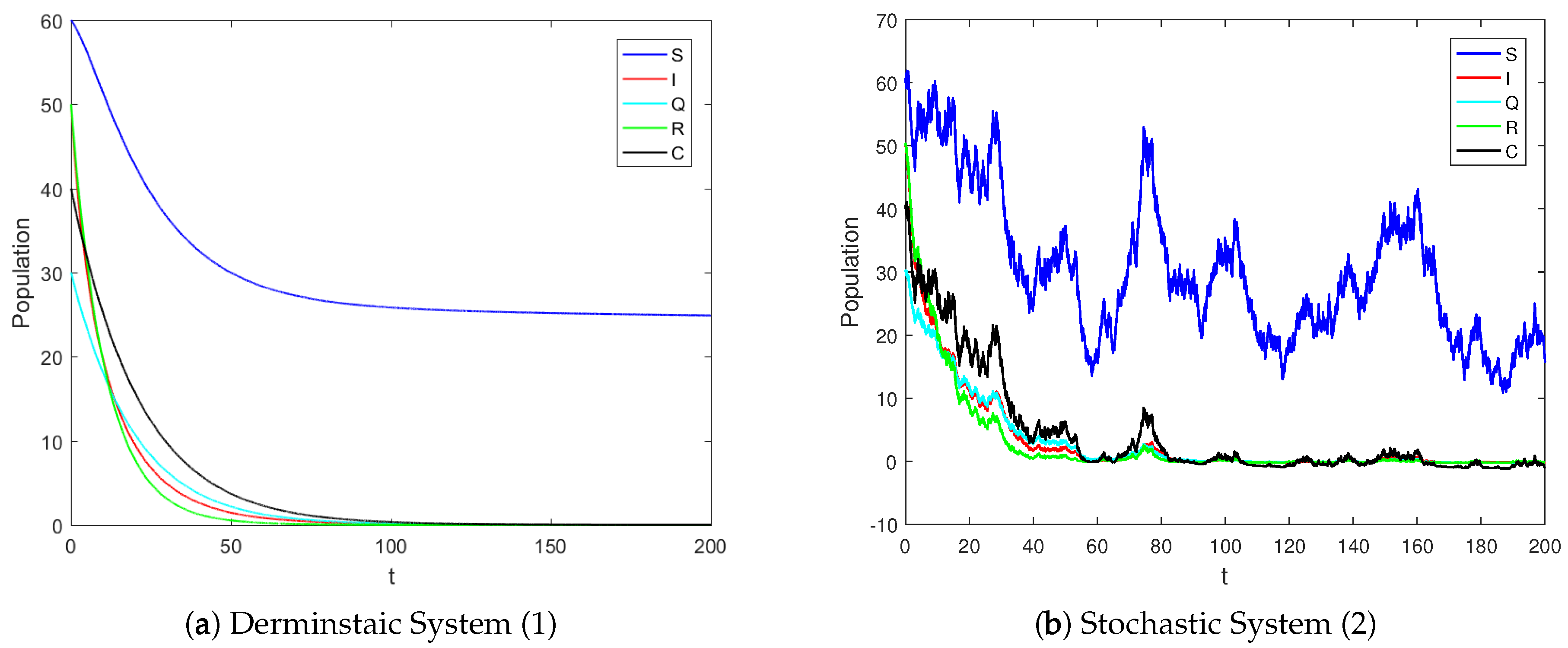
Model simulation is meant to validate the model’s projections or the hypothetical conclusion of the research in real-world scenarios, which is particularly important when modeling biological processes. In this part of the manuscript, the researchers strove to approximate the solutions of Model (2) by using classic computational methods that are rapidly convergent. The results of the significant proportion of the work that was based on the qualitative study were quantitatively validated. We quantitatively verified the theoretical predictions by using the standard RK-4 technique.

In order to obtain meaningful biological interpretations and quantitatively validate the abstract concepts, it is necessary to acquire the actual parameter values used in Model (2). In Examples 1 and 2, we presumed two sets of parameter values for this goal, and the initial sizes of the human populations and the concentration of the COVID-19 viruses are also presented. In each case, the simulation took place in the interval of time from 0 to 250.

We established Theorem 2 specifically considering the stochastic stability theory, which demonstrates that, under $R_s<1$, the disease will seem to be eradicated outside the community no matter what the initial sizes of the states are. Furthermore, the theorem indicates that COVID-19 will be surely eradicated from the population. Figure 3 shows that the graphs of the stochastic solutions will reach the infection-free equilibrium within a finite time period, confirming the theoretical results.

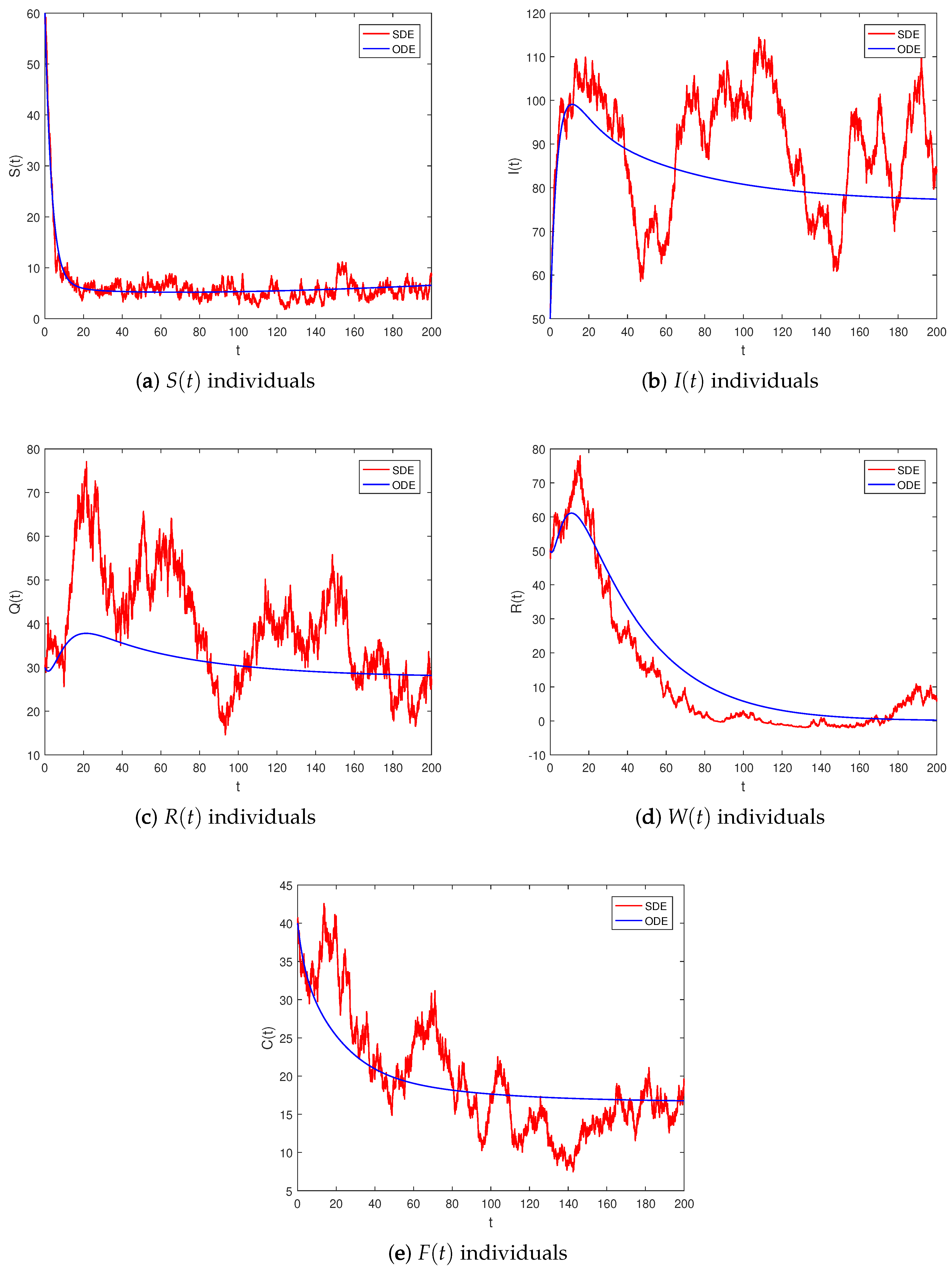
Likewise, Theorem 3 guarantees the virus’s pervasiveness in the community under some reasonable condition(s). By using the data from Example 2, we calculated the threshold, ${\mathbf{R}}_{\mathbf{0}}^{\mathbf{s}}$, and noticed that the value exceeded unity. Figure 4 depicts the simulated findings of the model predicated in light of the corresponding theorems. The figure indicates that the disease will continue to exist within the population, and it also illustrates the phenomenon of persistence demonstrated by Model (2). This proves Theorem 3’s judgments for the underlying deterministic model (1). Whenever the threshold of the corresponding stochastic model is greater than 1, the solution curves of the SDE model (2) go up and down all around the nonzero equilibrium point. As a result, efforts should concentrate on implementing effective prevention programs against the various variants to control the spread of multiple strains and the shedding of the virus in the community.

Example 1.

To simulate the model, we let the values of the parameters be as follows: $\omega =0.09,\Pi =0.12,\beta =0.002,\mu =0.005,{\alpha }_1=0.2,\eta =0.004,\delta =0.005,$ and $d=0.05$, where the initial size of each compartment was $\mathbb{S}\left(0\right)=60,\mathbb{I}\left(0\right)=50,\mathbb{Q}\left(0\right)=30,\mathbb{R}\left(0\right)=50,\mathbb{C}\left(0\right)=40$. Similarly, the intensities of the white noises were: ${\xi }_1=0.55,{\xi }_2=0.25,{\xi }_3=0.25,{\xi }_4=0.33,{\xi }_5=0.55$. Using all these model parameters, we determined $R_s$, which was found to be somewhere between zero and one. As a result, Theorem 2’s assumption was satisfied, and the element of the solution to the proposed system adhered to the following assertions:

$$\underset{t\to \infty }{lim}sup\frac{\log \mathbb{I}\left(t\right)}{t}\le 0,a.s.$$

$$\underset{t\to \infty }{lim}sup\frac{\log \mathbb{C}\left(t\right)}{t}\le 0,a.s.$$

Biologically, these relations describe the eradication of COVID-19 from the population, and numerically, this was confirmed via Figure 3. As a direct consequence, the acquired results of the analysis on extinction are accurate and reliable.

Example 2.

Here, the values of the parameters are given by: $\omega =0.07,\Pi =2.12,\beta =0.008,\mu =0.001,{\alpha }_1=0.2,\eta =0.004,\delta =0.005,$ and $d=0.08$. In the same way, we have the initial size of each compartment as: $\mathbb{S}\left(0\right)=80,\mathbb{I}\left(0\right)=50,\mathbb{Q}\left(0\right)=0,\mathbb{R}\left(0\right)=10,\mathbb{C}\left(0\right)=10$, whereas the intensities are given by ${\xi }_1=0.50,{\xi }_2=0.35,{\xi }_3=0.70,{\xi }_4=0.50,{\xi }_5=0.41$. Based on this information, we calculated the value of ${\mathbb{R}}_0^s$, which was found to be higher than 1. We also investigated whether the model parameters in this example satisfy the assumption of Theorem 3. The model’s solution was approximated using this example, and the results are shown in the diagram in Figure 4. The figure demonstrates that the virus is likely to persist in the community, and the system will have a steady-state distribution in this scenario.

The Impact of $\beta$ on the Stochastic System (2)

Let us consider $\beta =0.009$ and initial condition $\mathbb{S}\left(0\right)=60,\mathbb{I}\left(0\right)=40,\mathbb{Q}\left(0\right)=30,\mathbb{R}\left(0\right)=50,\mathbb{C}\left(0\right)=300$ with different stochastic noises ${\xi }_1=0.40,{\xi }_2=0.45,{\xi }_3=0.30,{\xi }_4=0.35,{\xi }_5=0.45$, and the remaining values were kept the same as used to generate Figure 4. Figure 5 depicts the relevant partial solutions $\mathbb{I},\mathbb{C}$, and the mean infection proportional cure of the stochastic system (2) with its associated deterministic model. It was evident that, as the random variability of individuals in the $\mathbb{I}$ and $\mathbb{C}$ classes increased, all infected individuals would eventually disappear from the population within a finite period of time. This suggests that, by limiting the value of $\beta$, we can regulate and avoid COVID-19 in the long term. Assuming that the stochastic disturbances are significant enough and the transmission coefficients are decreased, the disease can be eliminated.

8. Concluding Remarks and Future Directions

In this manuscript, the researchers investigated a new dynamic model for the spread of the COVID-19 epidemic, which is produced by the virus persisting in the air and surfaces due to ventilation, temperature, and humidity. It was proven that the proposed stochastic COVID-19 model was biologically justified by showing the existence, uniqueness, and positivity of the solution. It was explored whether the model had a global unique solution. We derived sufficient results both for the persistence and extinction of COVID-19. It was observed that, for $R_s^0>1$, the persistence of the disease occurred, and it was found that, if $R_s<1$, the COVID-19 infection would eventually be eliminated from the population. Supplementary graphs were represented, which showed the behavior of the solutions to the model, in particular the long-term behavior. This research could provide a solid theoretical foundation for a profound comprehension of prolonged contagious diseases. Our work was also intended to provide general techniques for developing the Lyapunov functions that will help the readers explore the stationary distribution of stochastic models having perturbations of the nonlinear type in particular.

COVID-19’s propagation via contaminated surfaces and the air is restricted by ventilation, humidity, and temperature, which were observed to be more pertinent than human-to-human COVID-19 transfer. Nevertheless, the investigators suggested that, in order to significantly reduce the risk, all of these elements should be monitored simultaneously. In future work, the authors hope to incorporate more appropriate characteristics of COVID-19 into the model, such as age and spatial effects. It is also being considered to incorporate various uptake functions into the frameworks in the coming years.