An Evolutionary View on Equilibrium Models of Transport Flows

Abstract

In this short paper, we describe natural logit population games dynamics that explain equilibrium models of origin-destination matrix estimation and (stochastic) traffic assignment models (Beckmann, Nesterov–de Palma). Composition of the proposed dynamics allows to explain two-stages traffic assignment models.

1. Introduction

The first traffic assignment model was proposed for about 70 years ago in the work of M. Beckmann [1], see also [2]. Nowadays Beckmann’s type models are rather well studied [3,4,5,6,7]. The entropy-based origin–destination matrix models are also well developed nowadays [7,8,9]. Moreover, as was mentioned in [10], both of these two types of models can be considered as macrosystem equilibrium for logit (best-response) dynamics in corresponding congestion games [11].

In this paper, we popularise the results of [10] for English-reading people (The paper [10] was written in Russian and has not been translated yet) and refine the results on the convergence rate. Moreover, we propose superposition of the considered dynamics to describe equilibrium in two-stage traffic assignment model [12,13].

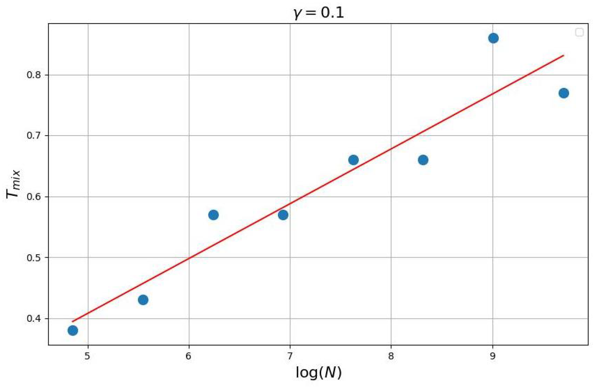
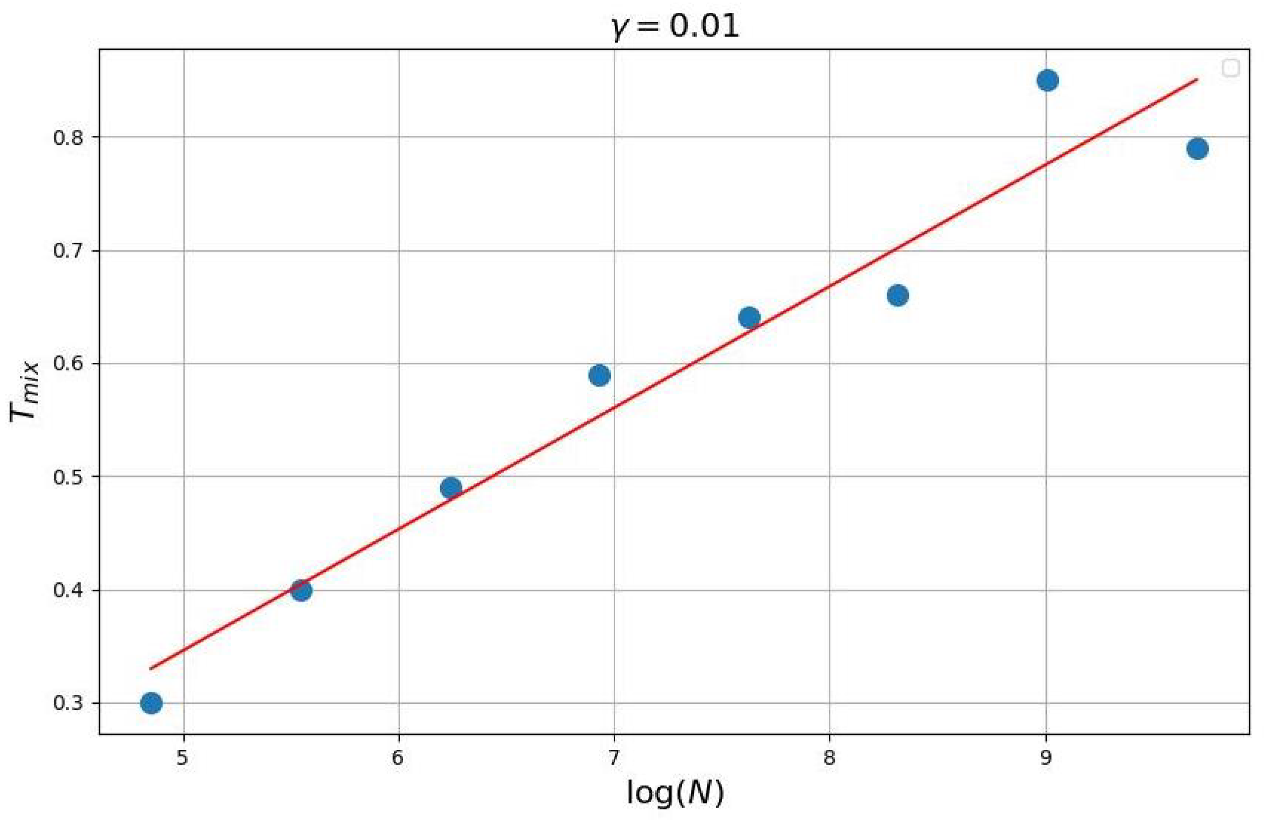
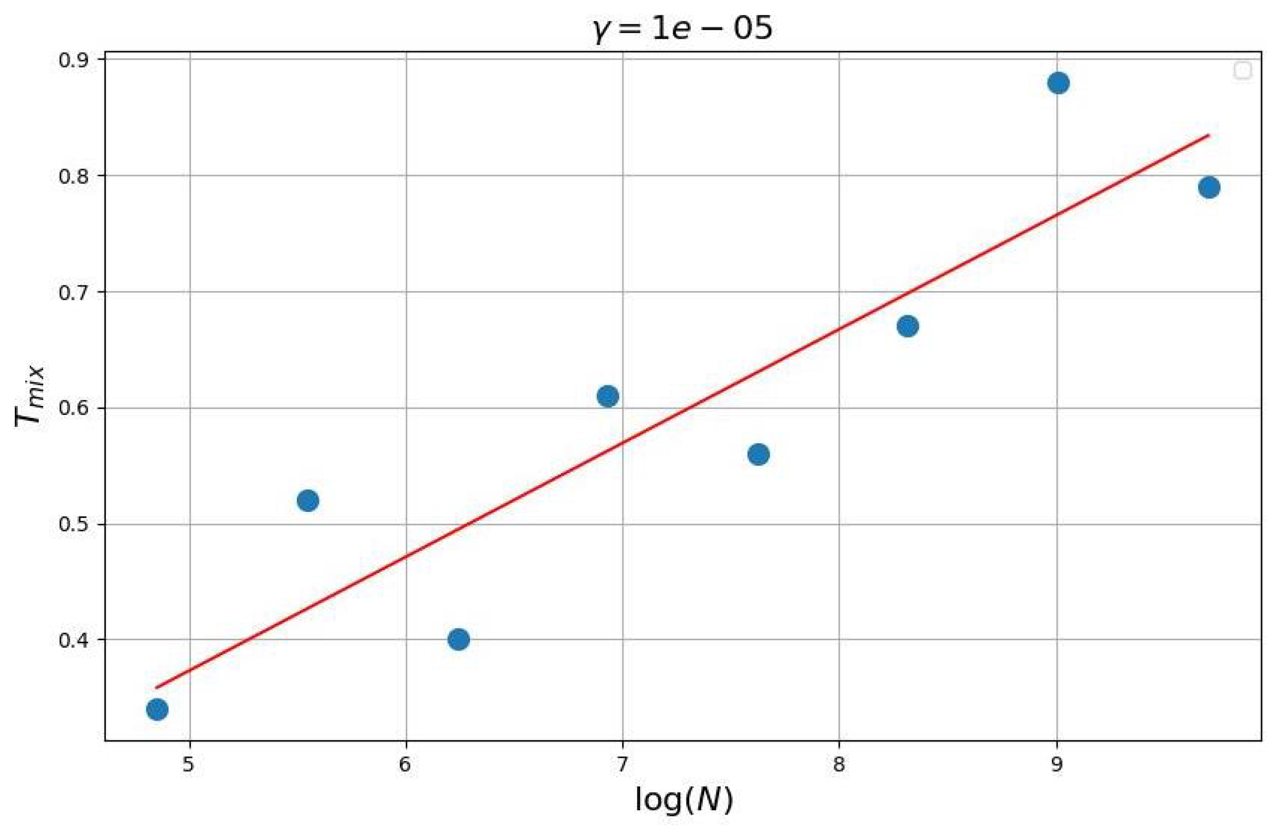
One of the main results of the paper is Theorem 1, where it is proved that the natural logit-choice and best-response Markovian population dynamics in traffic assignment model (congested population game) converge to equilibrium. By using Cheeger’s inequality we first time show that mixing time (the time required to reach equilibrium) of these dynamics $T_{mix}$ is proportional to $lnN$, where N is a total number of agents. Note, that in related works analogues of this theorem were proved without estimating of $T_{mix}$ [9,11,13]. We confirm Theorem 1 by numerical experiments.

Another important result is a saddle-point reformulation of two-stages traffic assignment model. We explain how to apply results of Theorem 1 to this model.

2. Traffic Assignment: Problem Statement

Following [14] we describe the problem statement.

Let the urban road network be represented by a directed graph $G=(V,E)$, where vertices V correspond to intersections or centroids [4] and edges E correspond to roads, respectively. Suppose we are given the travel demands: namely, let $d_w$ (veh/h) be a trip rate for an origin–destination pair w from the set $OD\subseteq \{w=(i,j):i\in O,j\in D\}$. Here, $O\subseteq V$ is the set of all possible origins of trips, and $D\subseteq V$ is the set of destination nodes. For OD pair $w=(i,j)$ denote by $P_w$ the set of all simple paths from i to j. Respectively, $P={\bigcup }_{w\in OD}{P}_w$ is the set of all possible routes for all OD pairs. Agents travelling from node i to node j are distributed among paths from $P_w$, i.e., for any $p\in P_w$ there is a flow $x_p\in {\mathbb{R}}_{+}$ (i.e., $x_p\ge 0$) along the path p, and ${\sum }_{p\in P_w}{x}_p=d_w$. Flows from vertices from the set O to vertices from the set D create the traffic in the entire network G, which can be represented by an element of

$$X=X\left(d\right)=\left\{x\in {\mathbb{R}}_{+}^{\left|P\right|}:\sum _{p\in P_w}{x}_p=d_w,w\in OD\right\}.$$

Note that set X can have extremely large number of paths (routes): e.g., for $n\times n$ Manhattan network $log\left|P\right|=\mathsf{\Omega }\left(n\right)$ up to a logarithmic factor. Note, that to describe a state of the network we do not need to know an entire vector x, but only flows on arcs: $f_e\left(x\right)={\sum }_{p\in P}{\delta }_{ep}{x}_p\mathrm{for}e\in E$, where ${\delta }_{ep}=\mathbb{1}\{e\in p\}$. Let us introduce a matrix $\mathsf{\Theta }$ such that ${\mathsf{\Theta }}_{e,p}={\delta }_{ep}$ for $e\in E$, $p\in P$, so in vector notation we have $f=\mathsf{\Theta }x$. To describe an equilibrium we use both path- (route-) and link-based notations $(x,t)$ or $(f,t)$.

Beckmann model. An important idea behind the Beckmann model is that the cost (e.g., travel time) of passing a link e is the same for all agents and depends only on the flow $f_e$ along it. We denote this cost for a given flow $f_e$ by $t_e={\tau }_e\left(f_e\right)$. Another essential point is a behavioral assumption (the first Wardrop’s principle): each agent knows the state of the whole network and chooses a path p minimizing the total cost $T_p\left(t\right)={\sum }_{e\in p}{t}_e.$

We consider ${\tau }_e\left(f_e\right)$ to be continuous, non-decreasing, and non-negative. In this case $\left(x^{*}={\left(x_p^{*}\right)}_{p\in P},t^{*}={\left(t_e^{*}\right)}_{e\in E}\right)$, is an equilibrium state, i.e., it satisfies conditions

$$\begin{array}{c}{t}_e^{*}={\tau }_e\left(f_e^{*}\right),\mathrm{where}{f}^{*}=\mathsf{\Theta }{x}^{*},\\ x_{p_w}^{*}>0⟹T_{p_w}\left(t^{*}\right)=T_w\left(t^{*}\right)=\underset{p\in P_w}{min}{T}_p\left(t^{*}\right),\end{array}$$

if, and only if, $x^{*}$ is a minimum of the potential function:

$$\begin{array}{c}\hfill \mathsf{\Psi }\left(f\left(x\right)\right)=\sum _{e\in E}\underset{{\sigma }_e\left(f_e\right)}{\underbrace{{\int }_0^{f_e}{\tau }_e\left(z\right)dz}}⟶\underset{f=\mathsf{\Theta }x,x\in X}{min}\\ \hfill ⟺\mathsf{\Psi }\left(f\right)=\sum _{e\in E}{\sigma }_e\left(f_e\right)⟶\underset{f=\mathsf{\Theta }x:x\in X}{min},\end{array}$$

and $t_e^{*}={\tau }_e\left(f_e^{*}\right)$ [2].

According to [5,13], we can construct a dual problem for the potential function in the following way:

$$\begin{array}{cc}\hfill \underset{f=\mathsf{\Theta }x:x\in X}{min}\mathsf{\Psi }\left(f\right)& =\underset{x\in X,f}{min}\left[\mathsf{\Psi }\left(f\right)+\underset{t\in {\mathbb{R}}^{\left|E\right|}}{sup}\langle t,\mathsf{\Theta }x-f\rangle \right]=\underset{t\in {\mathbb{R}}^{\left|E\right|}}{sup}\underset{x\in X,f}{min}\left[\mathsf{\Psi }\left(f\right)+\langle t,\mathsf{\Theta }x-f\rangle \right]\hfill \\ \hfill & =\underset{t\in {\mathbb{R}}^{\left|E\right|}}{sup}\left[-\sum _{e\in E}\underset{f_e}{max}\{t_e{f}_e-{\sigma }_e\left(f_e\right)\}+\underset{x\in X}{min}\sum _{p\in P}\sum _{e\in E}{t}_e{\delta }_{ep}{x}_p\right]\hfill \\ \hfill & =\underset{t\in dom{\sigma }^{*}}{max}-\left[\sum _{e\in E}{\sigma }_e^{*}\left(t_e\right)-\sum _{w\in OD}{d}_w{T}_w\left(t\right)\right],\hfill \end{array}$$

where

$${\sigma }_e^{*}\left(t_e\right)=\underset{f_e\ge 0}{sup}\{t_e{f}_e-{\sigma }_e\left(f_e\right)\}={\overline{f}}_e{\left(\frac{t_e-{\overline{t}}_e}{{\overline{t}}_e\rho }\right)}^{\mu }\frac{\left(t_e-{\overline{t}}_e\right)}{1+\mu }$$

is the Legendre—Fenchel conjugate function of ${\sigma }_e\left(f_e\right)$, $e\in E$. At the end we obtain the dual problem, which solution is $t^{*}$:

$$\underset{t\ge \overline{t}}{max}\left\{\sum _{w\in OD}{d}_w{T}_w\left(t\right)-\sum _{e\in E}{\sigma }_e^{*}\left(t_e\right)\right\}.$$

(1)

We can reconstruct primal variable f from the current dual variable t:

$$f\in \partial \sum _{w\in OD}{d}_w{T}_w\left(t\right).$$

This condition reflects the fact that every driver choose the shortest route [5]. Another condition $t_e={\tau }_e\left(f_e\right)$ can be equivalently rewrite as $f_e=\frac{d}{d{t}_e}{\sigma }_e^{*}\left(t_e\right)$. This condition with the condition $f\in \partial {\sum }_{w\in OD}{d}_w{T}_w\left(t\right)$ form the optimization problem (1).

If $\mu \to 0+$ Beckmann’s model will turn into Nesterov–de Palma model [13,15].

Population games dynamic for (stochastic) Beckmann model. Let us consider each driver to be an agent in population game, where $P_w$, $w\in OD$ is a set of types of agents. All agent (drivers) of type $P_w$ can choose one of the strategy $p\in P_w$ with cost function $T_p\left(t\left(f\left(x\right)\right)\right):={\tilde{T}}_p\left(x\right)$. Assume that every driver/agent independently of anything (in particular of any other drivers) is considering the opportunity to reconsider his choice of route/strategy p in time interval $[\mathrm{t},\mathrm{t}+\mathsf{\Delta }\mathrm{t})$ with probability $\lambda \mathsf{\Delta }\mathrm{t}+o\left(\mathsf{\Delta }\mathrm{t}\right)$, where $\lambda >0$ is the same for all drivers/agents. It means that with each driver we relate its own Poisson process with parameter $\lambda$. If in moment of time t (when the flow distribution vector is $x\left(\mathrm{t}\right)$) the the driver of type $P_w$ decides to reconsider his route, than he choose the route $q\in P_w$ with probability

$$p_q\left(\tilde{T}\left(x\left(\mathrm{t}\right)\right)\right)=\mathbb{P}\left(q=\underset{p\in P_w;j=1,\dots ,J}{arg\; max}\left\{-{\tilde{T}}_p\left(x\left(\mathrm{t}\right)\right)+{\xi }_{p,j}\right\}\right),$$

(2)

where ${\xi }_{p,j}$ are i.i.d. and satisfy Gumbel max convergence theorem [16] when $J\to \infty$ with the parameter $\gamma$ (e.g., ${\xi }_{p,j}$ has (sub)exponential tails at ∞). It means that ${\xi }_p={max}_{j=1,\dots ,J}{\xi }_{p,j}$ asymptotically (when $J\to \infty$) has Gumbel distribution $\mathbb{P}\left({\xi }_p<\xi \right)=exp\left(-exp\left(-\xi /\gamma -E\right)\right)$, where $E\simeq 0.5772$ is Euler constant. Note that $\mathbb{E}{\xi }_p=0$, $\mathrm{Var}{\xi }_p={\pi }^2{\gamma }^2/6$. In (2) it means that every driver try to choose the best route. However, the only available information are noise corrupted values ${\tilde{T}}_p$. So the driver try to choose the best route focused on the worst forecasts for each route.

One of the main results of Discrete Choice Theory is as follows [17]

$$p_q\left(\tilde{T}\left(x\left(\mathrm{t}\right)\right)\right)=\frac{exp\left(-{\tilde{T}}_p\left(x\left(\mathrm{t}\right)\right)/\gamma \right)}{{\sum }_{q\in P_w}exp\left(-{\tilde{T}}_q\left(x\left(\mathrm{t}\right)\right)/\gamma \right)},$$

(3)

where $p_q\left(\tilde{T}\left(x\left(\mathrm{t}\right)\right)\right)$ was previously defined in (2).

Note that the described above dynamic degenerates into the best-response dynamic when $\gamma \to 0+$ [11].

Theorem 1.

Let ${\sum }_{p\in P}{x}_p=N$. For all $x\left(0\right)\in X$ there exists such a constant $c\left(x\left(0\right)\right)$ that for all $\sigma \in \left(0,0.5\right)$ and $\mathrm{t}\ge T_{mix}=c\left(x\left(0\right)\right){\lambda }^{-1}lnN$:

$$\mathbb{P}\left({∥\frac{x\left(\mathrm{t}\right)}{N}-x^{*}∥}_2\le \frac{2\sqrt{2}+4\sqrt{ln\left({\sigma }^{-1}\right)}}{\sqrt{N}}\right)\ge 1-\sigma ,$$

(4)

where

$$x^{*}=\underset{x\in X\left(d/N\right)}{arg\; min}\left\{\tilde{\mathsf{\Psi }}\left(f\left(x\right)\right)+\gamma \sum _{p\in P}{x}_{p}ln{x}_p\right\},$$

(5)

$$\tilde{\mathsf{\Psi }}\left(f\left(x\right)\right)={\sum }_{e\in E}{\int }_0^{f_e}{\tilde{\tau }}_e\left(z\right)dz, {\tilde{\tau }}_e\left(z\right)={\tau }_e\left(zN\right).$$

Proof. 

The first important observation is that the described Markov process is reversible. That is, it satisfies Kolmogorov’s detailed balance condition (see also [18]) with stationary (invariant) measure

$$\pi \left(x\right)=\frac{N!}{x_1!\dots x_{\left|P\right|}!}exp\left(-\frac{\mathsf{\Psi }\left(f\left(x\right)\right)}{\gamma }\right),$$

where $x\in X\left(d\right)$ [11]. The result of type (4) for $x(\infty )$ holds true due to Hoeffding’s inequality in a Hilbert space [19]. We can apply this inequality for multinomial part $\frac{N!}{x_1!\dots x_{\left|P\right|}!}$. The rest part may only strength the concentration phenomenon, especially when $\gamma$ is small. The Sanov’s theorem [20] says that $x^{*}$ from (5) asymptotically ($N\to \infty$) describe the proportions in maximum probability state, that is

$$x^{*}N\simeq \underset{x\in X\left(d\right)}{arg\; max}\frac{N!}{x_1!\dots x_{\left|P\right|}!}exp\left(-\frac{\mathsf{\Psi }\left(f\left(x\right)\right)}{\gamma }\right).$$

To estimate the mixing time $\sim {\lambda }^{-1}lnN$ of the considered Markov process we will put it in accordance with this continuous-time process discrete-time process with step ${\left(\lambda N\right)}^{-1}$, which corresponds to the expectation time between two nearest events in continuous-time dynamic. Additionally, we consider this discrete Markov chain as a random walk on a proper graph $G=\langle V_G,E_G\rangle$ with starting point corresponds to the vertex s and transition probability matrix $P=\parallel p_{ij}{\parallel }_{i,j=1}^{|V_G|}$. According to a Cheeger’s inequality mixing time ${\mathrm{t}}_{\mathrm{mix}}$ for such a random walk, which approximate stationary measure $\pi$ with accuracy $\epsilon =O\left(N^{-1/2}\right)$ (in this case $x\left({\mathrm{t}}_{\mathrm{mix}}\right)\simeq x(\infty )$), is

$$O\left({\left(\lambda N\right)}^{-1}h{\left(G\right)}^{-2}\left(ln\left(\pi \left(s\right)\right)+ln\left({\epsilon }^{-1}\right)\right)\right),$$

where Cheeger’s constant is determined as

$$h\left(G\right)=\underset{S\subseteq V_G:\pi \left(S\right)\le 1/2}{min}\mathbb{P}\left(S\to \overline{S}\mid S\right)=\underset{S\subseteq V_G:\pi \left(S\right)\le 1/2}{min}\frac{{\sum }_{(i,j)\in E_G,i\in S,j\in \overline{S}}\pi \left(i\right)p_{ij}}{{\sum }_{i\in S}\pi \left(i\right)},$$

where $\overline{S}=V_G/S$ [21]. Since G and P correspond to reversible Markov chain with stationary measure $\pi$ that exponentially concentrate around $x^{*}N$ one can prove that isoperimetric problem of finding optimal set of vertexes S has the following solution, which we described below roughly up to a numerical constant: S is a set of such states $x\in X\left(d\right)$ that $\parallel x-x^{*}{N\parallel }_2\lesssim O\left(\sqrt{N}\right)$. Since the the ratio of sphere volume of radius $O\left(\sqrt{N}\right)$ to the volume of the ball of the same radius is $O\left(N^{-1/2}\right)$, we can obtain that $h\left(G\right)\sim N^{-1/2}$. So up to a $ln\left(\pi \left(s\right)\right)$ (we put it into $c\left(x\left(0\right)\right)$) mixing time is indeed $\sim {\lambda }^{-1}lnN$. □

Note that the describe above approach assumes that we first $\mathrm{t}\to \infty$ and then $N\to \infty$. If we firstly take $N\to \infty$ than due to Kurtz’s theorem [22] $c\left(\mathrm{t}\right)={lim}_{N\to \infty }x\left(\mathrm{t}\right)/N$ satisfies (for all $w\in OD$, $p\in P_w$)

$$\frac{d{c}_p}{dt}={\overline{d}}_w\frac{exp\left(-{\overline{T}}_p\left(c\left(\mathrm{t}\right)\right)\right)}{{\sum }_{q\in P_w}exp\left(-{\overline{T}}_q\left(c\left(\mathrm{t}\right)\right)\right)}-c_p\left(\mathrm{t}\right),$$

where $\overline{d}={lim}_{N\to \infty }d/N$, ${\overline{T}}_p\left(c\left(\mathrm{t}\right)\right)={\tilde{T}}_p\left(x\left(\mathrm{t}\right)\right)$. Note that Sanov’s type function $\tilde{\mathsf{\Psi }}\left(f\left(c\right)\right)+\gamma {\sum }_{p\in P}{c}_{p}ln{c}_p$ from (5) will be Boltzmann–Lyapunov type function for this system of ordinary differential equations (SODE), that is decrees along the trajectory of SODE. This result is a particular case of the general phenomenon: Sanov’s type function for invariant measure obtained from Markovian dynamics is Boltzmann–Lyapunov type function for deterministic Kurtz’s kinetic dynamics [18,23,24].

3. Origin–Destination Matrix Estimation

Origin–destination matrix estimation model can be considered as a particular case of the traffic assignment model. The following interpretation goes back to [10,13]. Indeed, let us consider fictive origin o and fictive destination d. So $\tilde{O}=\left\{o\right\}$, $\tilde{D}=\left\{d\right\}$. Let us draw fictive edges from o to real origins of trips O. The cost of the trip at edge $(o,i)$ is ${\lambda }_i^O$—an average price that each agent pays to live at this origin region $i\in O$. Analogously, let us draw edges from the vertexes of the real destination set D to d. The cost of the trip at edge $(j,d)$ is $-{\lambda }_j^D$, minus average salary that each agent obtains in destination region $j\in D$. So the set of all possible routes (trips) from o to d can be described by pairs $(i,j)\in OD$. Each route consist of three edges $o\to i$ with cost ${\lambda }_i^O$, edge $i\to j$ with cost $T_{ij}$ (is available as an input of the model) and edge $j\to d$ with cost $-{\lambda }_j^D$. So equilibrium origin-destination matrix $d={\left\{d_{ij}\right\}}_{(i,j)\in OD}$ (up to a scaling factor) can be find from entropy-linear programming problem

$$\underset{d\ge 0:{\sum }_{(i,j)\in OD}{d}_{ij}=1}{min}\sum _{i\in O}{\lambda }_i^O\sum _{j\in D}{d}_{ij}-\sum _{j\in D}{\lambda }_j^D\sum _{i\in O}{d}_{ij}+\sum _{(i,j)\in OD}{T}_{ij}{d}_{ij}+\gamma \sum _{(i,j)\in OD}{d}_{ij}ln{d}_{ij}.$$

(6)

In real life, ${\lambda }_i^O$ and ${\lambda }_j^D$ are typically unknown. However, at the same time, the following agglomeration characters are available

$$\sum _{j\in D}{d}_{ij}=L_i,i\in O,$$

(7)

$$\sum _{i\in O}{d}_{ij}=W_j,j\in D.$$

(8)

The key observation is that (6) can be considered as Lagrange multipliers principle for constraint entropy-linear programming problem

$$\underset{d\ge 0:d\mathrm{satisfies}\left(7\right),\left(8\right)}{min}\sum _{w\in OD}{T}_w{d}_w+\gamma \sum _{w\in OD}{d}_{w}ln{d}_w,$$

(9)

where ${\lambda }_i^O$ and ${\lambda }_j^D$ are Lagrange multipliers for (7) and (8) correspondingly. The last model is called Wilson’s entropy origin–destination matrix model [8,9].

The result of Theorem 1 can be applied to this model due to the mentioned above reduction.

4. Two-Stages Traffic Assignment Model

From the Section 2 we may know that Beckmann’s model requires origin-destination matrix as an input ${\left\{d_w\right\}}_{w\in OD}$. So Beckmann’s model allows to calculate $t\left(d\right)$. At the same time, from Section 3, we may know that Wilson’s entropy origin–destination model requires cost matrix ${\left\{T_w\right\}}_{w\in OD}$ as an input, where $T_w:=T_w\left(t\right)={min}_{p\in P_w}{T}_p\left(t\right)$. So Wilson’s model allows to calculate $d\left(T\left(t\right)\right)$. The solution of the system $d=d\left(T\left(t\left(d\right)\right)\right)$ is called two-stage traffic assignment model [12]. Following [7,13] we can reduce this problem to the following one (see (1) and (9))

$$\underset{d\ge 0:d\mathrm{satisfies}\left(7\right),\left(8\right)}{min}\left\{\underset{t\ge \overline{t}}{max}\left\{\sum _{w\in OD}{d}_w{T}_w\left(t\right)-\sum _{e\in E}{\sigma }_e^{*}\left(t_e\right)\right\}+\gamma \sum _{w\in OD}{d}_{w}ln{d}_w\right\}.$$

(10)

The problem (10) can be rewritten as a convex-concave (if ${\tau }_e^{\prime }\left(t_e\right)\ge 0$) saddle-point problem (SPP)

$$\underset{d\ge 0:d\mathrm{satisfies}\left(7\right),\left(8\right)}{min}\underset{t\ge \overline{t}}{max}\left\{\sum _{w\in OD}{d}_w{T}_w\left(t\right)-\sum _{e\in E}{\sigma }_e^{*}\left(t_e\right)+\gamma \sum _{w\in OD}{d}_{w}ln{d}_w\right\}.$$

(11)

This SPP can be efficiently solved numerically [7].

Note that, if we consider best-response dynamics from Section 2, with the parameter $\lambda :={\lambda }_{\mathrm{Beck}}$ and logit dynamic with the parameter $\lambda :={\lambda }_{\mathrm{Wil}}$ for the origin–destination matrix estimation and assume that ${\lambda }_{\mathrm{Beck}}\gg {\lambda }_{\mathrm{Wil}}$ than such a dynamic will converge to the stationary (invariant) measure that is concentrated around the solution of the SPP problem (11). This result can be derived from the more general result related with hierarchical congested population games [7].

5. Numerical Experiments

The main result of the paper is Theorem 1. The main new result of this theorem is a statement that mixing time of the considered Markovian logit-choice and best-response dynamics $T_{mix}$ is approximately $c_1+c_2·lnN$, where N is a number of agents.

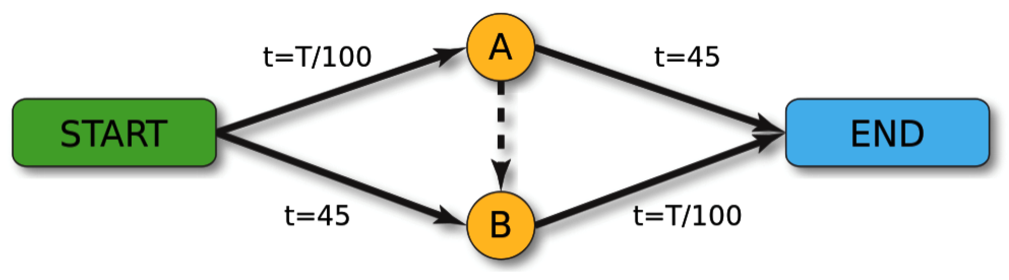
We consider Braess’s paradox example [25], see Figure 1. This picture is taken from Wikipedia. Here, Origin is START and Destination is END. We have one OD-pair and put $d=N$, the number of agents. The <<paradox>> arises when $N=4000$. In this case when there is no road from A to B we have two routes (START, A, END) and (START, B, END) with 2000 agents at each route. So the equilibrium time costs at each route will be 65. When the road AB is present (this road has time costs 0) all agents will use the route (START, A, B, END) and this equilibrium has time costs 80. That is paradoxically larger than it was without road AB.

In series of experiments (see Figure 2, Figure 3 and Figure 4) the dependence of mixing time $T_{mix}$ from $lnN$ was investigated. Details see in https://github.com/ZVlaDreamer/transport_flows_project (accessed on 1 November 2022).

Numerical experiments confirm Theorem 1. Note that in [9] it was described a real-life experiment oraganized with MIPT students in Experimental Economics Lab. The students were agents and play in repeated Braess’s paradox game. The result of experiments from [9] is also well agreed with the described above numerical experiments.

6. Conclusions

In this paper, we investigate logit-choice and best-response population Markovian dynamics converges to equilibrium in corresponding traffic assignment model. We show that mixing time is proportional to logarithm from the number of agent. Numerical experiments confirm that the dependence is probably unimprovable. We also consider two-stage traffic assignment model and describe how to interpret equilibrium for this model in an evolutionary manner.