An Analysis of a Fractional-Order Model of Colorectal Cancer and the Chemo-Immunotherapeutic Treatments with Monoclonal Antibody

Abstract

The growth of colorectal cancer tumors and their reactions to chemo-immunotherapeutic treatment with monoclonal antibodies (mAb) are discussed in this paper using a system of fractional order differential equations (FDEs). mAb medications are still at the research stage; however, this research takes into account the mAbs that are already in use. The major goal is to demonstrate the effectiveness of the mAb medication Cetuximab and the significance of IL-2 levels in immune system support. The created model is broken down into four sub-systems: cell populations, irinotecan (CPT11) concentration for treatment, IL-2 concentration for immune system support, and monoclonal antibody Cetuximab. We show the existence and uniqueness of the initial value problem (IVP). After that, we analyze the stability of the equilibrium points (disease-free and co-existing) using the Routh–Hurwitz criteria. In addition, in applying the discretization process, we demonstrate the global stability of the constructed system around the equilibrium points based on specific conditions. In the end, simulation results were carried out to support the theory of the manuscript.

1. Introduction

One of the most frequent cancers in the world for both women and men is colorectal cancer [1]. Apart from various and mixed treatment procedures to minimize and eliminate the cancerous tissues, the immune system (IS) has an important impact during the treatment. Within this, additional treatment strategies are involved in cancer therapy, such as using monoclonal antibody drugs. While there are still many unresolved problems about the efficiency of monoclonal antibodies and their use, we believe that mixed therapy would be well understood by establishing mathematical models and analyzing the optimal treatment process using clinical data that might support theoretical and applied science studies. Several studies with various treatment strategies looked into tumor cells’ interaction with the immune system. Some of them are [2,3,4,5,6,7].

Other research mainly concentrated on the resources and dynamics of $CD{8}^{+}T$ populations [8,9,10], while some clinical and mathematical research explicitly focused on the use of monoclonal antibodies in vivo and in vitro [5,11,12]. To illustrate the utility and application of both monoclonal antibody concentrations and immunotherapy, it is important to depict tumor growth and treatment procedures in applied sciences such as mathematical models. Thus, by combining theory and application, we may properly comprehend the dynamic of the biological system.

De Pillis et al. established in [12] the tumor progression while taking into account the levels of doxorubicin and IL-2 in the bloodstream as well as the effects of various immune cells. The study in [2] included the addition of three immunological compartments, one compartment each measuring tumor density, chemotherapy medication, and concentration of IL-2. As previously stated in [3], they also address the kinetics of IL-2 and the IL-2 production with biological interactions. Irinotecan, a chemotherapeutic drug, and one of two monoclonal antibodies—cetuximab, which has FDA approval for colorectal cancer treatments, and panitumumab, which is still being tested in clinical trials—were modelled by the authors in [5]. Here, they introduced and simulated a new experimental dosing schedule that reduced the tumor size efficiently.

The dynamical behavior is expanded in this manuscript in light of the studies on immunotherapy and monoclonal antibody treatment that were previously mentioned. Since derivatives and integrals are defined for any real order, fractional calculus is an extension of conventional calculus. Fractional operators can more effectively depict systems with high-order dynamics and complicated nonlinear phenomena than standard derivatives and integrals in particular situations. This is due to two key factors. First, we are not limited to integer order and are free to choose any order for the derivative and integral operators. Second, fractional order derivatives are advantageous when the system has a long-term memory since they depend not only on current circumstances but also on the past [13,14,15,16].

Hence, fractional-order differential equations can more accurately depict a variety of complicated biological processes with nonlinear dynamics and long-term memory that cannot be theoretically expressed by ODEs. Additionally, the conversion of an ODE model into an FDE model needs to be precise in terms of differentiation order because even a small change can have a big impact on how the solutions behave [17,18,19,20,21,22,23].

The effectiveness of immunotherapy and monoclonal antibody medications are established in the section that follows, which also establishes a system of fractional-order differential equations that take colorectal cancer growth, irinotecan concentration in chemotherapy, and other factors into account.

The structure of this manuscript is as follows: A tumor growth of colorectal cancer and its response to chemo-immunotherapeutic treatment with monoclonal antibody (mAb) is formulated as a system of fractional order differential equation in Section 2, where we also prove the IVP’s uniqueness and existence. In Section 3, we analyze the local stability of both equilibrium points, while Section 4 represents the global stability of the equilibrium points based on specific conditions. At the end of the study, we used in vivo and in vitro clinical data to illustrate the simulation results.

2. A Fractional-Order Mathematical Model

In the initiated model, a colorectal cancer malignant cell population is introduced. The purpose of the study is to examine and present the effectiveness of various immune system-supporting supplements and the response of cancer tissues to monoclonal antibody therapy (mAb). In order to go through a painful and protracted therapy, the combined therapy concentrates on removing the cancer tissues and bolstering the immune system with supplements.

Thus, the system is defined with seven compartments:

• $T\left(t\right)$: colorectal cancer cells,
• $N\left(t\right)$: compartment of natural killer (N.K.),
• $C\left(t\right)$: the CD$8^{+}$T cell population,
• $L\left(t\right)$: lymphocytes population,
• $D\left(t\right)$: irinotecan concentration,
• $I\left(t\right)$: IL-2 concentration,
• $A\left(t\right)$: mAb Cetuximab concentration.

The mAb Cetuximab and the chemotherapeutic medication Irinotecan (CPT11) will be examined as therapies.

Below is the mathematical system of colorectal cancer with multi-modal therapy.

$$\left\{\begin{array}{l}{D}^{\alpha }\left(T\left(t\right)\right)=r\left(1-{\alpha }_{1}T\left(t\right)\right)T(t)-{\beta }_{1}N\left(t\right)T\left(t\right)-{\gamma }_{1}D\left(t\right)T\left(t\right)-\delta A\left(t\right)T\left(t\right)-\frac{{\mu }_{1}A\left(t\right)N\left(t\right)T\left(t\right)}{{\epsilon }_1+A\left(t\right)}-\frac{{\theta }_{1}C\left(t\right)T\left(t\right)}{{\omega }_{1}T\left(t\right)+C\left(t\right)}\hfill \\ D^{\alpha }\left(N\left(t\right)\right)={\mathsf{\Lambda }}_{1}C\left(t\right)+\rho \left(1-{\alpha }_{2}N\left(t\right)\right)N\left(t\right)+\frac{\tau I\left(t\right)N\left(t\right)}{{\omega }_2+I\left(t\right)}-\frac{{\mu }_{2}A\left(t\right)N\left(t\right)T\left(t\right)}{{\epsilon }_1+A\left(t\right)}-{\beta }_{2}N\left(t\right)T\left(t\right)-{\gamma }_{2}D\left(t\right)N\left(t\right)\hfill \\ D^{\alpha }\left(C\left(t\right)\right)=\left({\sigma }_{1}L\left(t\right)+{\sigma }_{2}N\left(t\right)\right)T\left(t\right)+\frac{{\theta }_{2}C\left(t\right)I\left(t\right)}{{\omega }_3+I\left(t\right)}-\frac{\xi L\left(t\right)C\left(t\right)I\left(t\right)}{\varrho +I\left(t\right)}-{\beta }_{3}T\left(t\right)C\left(t\right)-{\gamma }_{3}D\left(t\right)C\left(t\right)\hfill \\ D^{\alpha }\left(L\left(t\right)\right)={\mathsf{\Lambda }}_2-{\alpha }_{3}L\left(t\right)-{\gamma }_{4}D\left(t\right)L\left(t\right)\hfill \\ D^{\alpha }\left(D\left(t\right)\right)={\mathsf{\Lambda }}_3-{\alpha }_{4}D\left(t\right)\hfill \\ D^{\alpha }\left(I\left(t\right)\right)={\mathsf{\Lambda }}_{4}L\left(t\right)-{\alpha }_{5}I\left(t\right)+\frac{{\theta }_{3}C\left(t\right)I\left(t\right)}{{\omega }_4+I\left(t\right)}\hfill \\ D^{\alpha }\left(A\left(t\right)\right)={\mathsf{\Lambda }}_5-{\alpha }_{6}A\left(t\right)+\frac{{\mu }_{3}A\left(t\right)T\left(t\right)}{{\epsilon }_2+A\left(t\right)}.\hfill \end{array}\right.$$

(1)

and

$$T\left(0\right)=T_0,N\left(0\right)=N_0,C\left(0\right)=C_0,L\left(0\right)=L_0,D\left(0\right)=D_0, I\left(0\right)=I_0\mathrm{and} A\left(0\right)=A_0,$$

(2)

where the parameters are defined in $R^{+},\alpha \in (0,\left.1\right],$ $D^{\alpha }$ is the Caputo derivative, see [24,25], and $\left(T,N,C,L,D,I,A\right)\in {\mathbb{R}}_{+}^7$.

Table 1. Parametric explanation.

Notation	Description of Parameter	Equation
$r$	Growth rate of the cancer cells	$\frac{dT}{dt}$
${\alpha }_1$	Capacity rate of the tumor
${\beta }_1$	$N-T$ interaction
${\gamma }_1$	Irinotecan-influence tumor decrease
$\delta$	mAb-influence tumor decrease
${\theta }_1$	Immune system strength coefficient
${\omega }_1$	Half-maximal $CD{8}^{+}T$ cell effectiveness
${\mu }_1$	N.K. induced tumor death through mAb
${\epsilon }_1$	Concentration of mAb for a half-maximal increase in Cetuximab
${\Lambda }_1$	Natural killer cell generation from circulating lymphocytes	$\frac{dN}{dt}$
$\rho$	Natural cell turnover rate
${\alpha }_2$	Inverse of carrying capacity of N.K. cells
$\tau$	IL-2-induced N.K. cell proliferation
${\omega }_2$	Concentration of IL-2 for half-maximal N.K. cell proliferation
${\mu }_2$	N.K. cell death due to the tumor-mAb complex interaction
${\epsilon }_1$	Concentration of mAb for a half-maximal increase in Cetuximab
${\beta }_2$	N.K. cell death due to interaction with compartment $T$
${\gamma }_2$	N.K. depletion from chemotherapy toxicity
${\sigma }_1$	NK-lysed tumor cell debris activation of $CD{8}^{+}T$ cell cells	$\frac{dC}{dt}$
${\sigma }_2$	$CD{8}^{+}T$ cell production from circulating lymphocytes
${\theta }_2$	IL-2 induced CD8 +T-cell activation
${\omega }_3$	Concentration of IL-2 for half-maximal $CD{8}^{+}T$ cell activation
$\xi$	$CD{8}^{+}T$ cell self-limitation feedback coefficient
$\varrho$	Concentration of IL-2 to halve the magnitude of $CD{8}^{+}T$ cell self-regulation
${\beta }_3$	$CD{8}^{+}T$ cell death due to tumor interaction
${\gamma }_3$	$CD{8}^{+}T$ cell depletion from chemotoxicity
${\Lambda }_2$	Bone marrow lymphocyte synthesis	$\frac{dL}{dt}$
${\alpha }_3$	Lymphocyte turnover
${\gamma }_4$	Lymphocyte depletion from chemotherapy
${\Lambda }_3$	Concentration of irinotecan $\mathrm{m}\mathrm{g}/\mathrm{L}$ per day	$\frac{dD}{dt}$
${\alpha }_4$	Elimination of chemotherapy
${\Lambda }_4$	IL-2 production: CD$4^{+}$/naive $CD{8}^{+}T$ cells	$\frac{dI}{dt}$
${\alpha }_5$	IL-2 turnover
${\theta }_3$	IL-2 production: $CD{8}^{+}T$ cells
${\omega }_4$	Concentration of IL-2 for half-maximal $CD{8}^{+}T$ cell IL-2 production
${\Lambda }_5$	Amount of monoclonal antibodies injected $mg/l$ per day	$\frac{dA}{dt}$
${\alpha }_6$	Rate of mAb turnover
${\mu }_3$	Loss of available mAbs to bind to tumor cells
${\epsilon }_2$	Concentration of mAbs half-maximal binding

illustrates the descriptions of [2,3,11,12,26,27,28].

Definition 1 

([24]). Given a function $\phi \left(t\right)$, the fractional integral with order $\alpha >0$ is given by Abdel’s formula as

$$I_{\alpha }\phi \left(t\right)=\frac{1}{\Gamma \left(\alpha \right)}{\int }_0^x{\left(x-t\right)}^{\alpha -1}\phi \left(t\right)dt, x>0.$$

Definition 2 

([24]). Let $\phi :R^{+}\to R$ be a continuous function. The Caputo fractional derivative of order $\alpha \in \left(n-1,n\right),$, where $n$ is a positive integer and is defined as

$$D^{\alpha }\phi \left(t\right)=\frac{1}{\Gamma \left(n-\alpha \right)}{\int }_0^t\frac{{\phi }^{\left(n\right)}\left(s\right)}{{\left(t-s\right)}^{\alpha +1-n}}ds.$$

when $\alpha =n$, the derivatives are defined to be the usual $nth$ order derivatives.

Definition 3 

([25]). The Mittag-Leffler function of one variable is

$$E_{\alpha }\left(\lambda ,z\right)=E_{\alpha }\left(\lambda z^{\alpha }\right)={\sum }_{k=0}^{\infty }\frac{{\lambda }^k{z}^{\alpha k}}{\Gamma \left(1+\alpha k\right)},\left(\lambda \ne 0,z\in \mathbb{C};Re\left(\alpha \right)>0\right).$$

The existence of a positive domain ${\mathbb{R}}_{+}^7=\left\{\mathcal{M}\in {\mathbb{R}}^7:\mathcal{M}\ge 0\right\},$ where $\mathcal{M}\left(t\right)={\left(T\left(t\right),N\left(t\right),C\left(t\right),L\left(t\right),D\left(t\right),I\left(t\right),A\left(t\right)\right)}^T$, and the unique solution of an IVP in the same region ${\mathbb{R}}_{+}^7$ can be shown using the lemma and theory in [29,30,31]. The local stability analysis of both equilibrium points—disease-free and coexisting—will serve as the foundation for our main research in the following part.

Theorem 1. 

The solution of the IVP in (1) and (2) is unique, and the solutions are in ${\mathbb{R}}_{+}^7$.

Proof of Theorem 1. 

Using the lemma and theory in [29,30,31], we have to prove that the domain ${\mathbb{R}}_{+}^7$ is positively invariant. Thus, we have the following:

$$\begin{array}{l}{\left.D^{\alpha }\mathrm{T}\left(\mathrm{t}\right)\right|}_{T=0}=0,\hfill \\ {\left.D^{\alpha }\mathrm{N}\left(\mathrm{t}\right)\right|}_{N=0}={\Lambda }_{1}C\left(t\right)\ge 0,\hfill \\ {\left.D^{\alpha }\mathrm{C}\left(\mathrm{t}\right)\right|}_{C=0}=\left({\sigma }_{1}L\left(t\right)+{\sigma }_{2}N\left(t\right)\right)T\left(t\right)\ge 0,\hfill \\ {\left.D^{\alpha }\mathrm{L}\left(\mathrm{t}\right)\right|}_{L=0}={\Lambda }_2>0,\hfill \\ {\left.D^{\alpha }\mathrm{D}\left(\mathrm{t}\right)\right|}_{D=0}={\Lambda }_3>0,\hfill \\ {\left.D^{\alpha }\mathrm{I}\left(\mathrm{t}\right)\right|}_{I=0}={\Lambda }_{4}L\left(t\right)\ge 0,\hfill \\ {\left.D^{\alpha }\mathrm{A}\left(\mathrm{t}\right)\right|}_{A=0}={\Lambda }_5>0.\hfill \end{array}$$

This implies that all the above equations are non-negative, which shows that the domain ${\mathbb{R}}_{+}^7$ is positively invariant. □

Let us rewrite the system:

$$\left\{\begin{array}{cc}{D}^{\alpha }T\left(\mathrm{t}\right)\hfill & =k_1\left(T\left(t\right),N\left(t\right),C\left(t\right),L\left(t\right),D\left(t\right),I\left(t\right),A\left(t\right)\right)\hfill \\ \hfill & =r\left(1-{\alpha }_{1}T\left(t\right)\right)T(t)-{\beta }_{1}N\left(t\right)T\left(t\right)-{\gamma }_{1}D\left(t\right)T\left(t\right)-\delta A\left(t\right)T\left(t\right)-\frac{{\mu }_{1}A\left(t\right)N\left(t\right)T\left(t\right)}{{\epsilon }_1+A\left(t\right)}-\frac{{\theta }_{1}C\left(t\right)T\left(t\right)}{{\omega }_{1}T\left(t\right)+C\left(t\right)}\hfill \\ D^{\alpha }\mathrm{N}\left(\mathrm{t}\right)\hfill & =k_2\left(T\left(t\right),N\left(t\right),C\left(t\right),L\left(t\right),D\left(t\right),I\left(t\right),A\left(t\right)\right)\hfill \\ \hfill & ={\Lambda }_{1}C\left(t\right)+\rho \left(1-{\alpha }_{2}N\left(t\right)\right)N\left(t\right)+\frac{\tau I\left(t\right)N\left(t\right)}{{\omega }_2+I\left(t\right)}-\frac{{\mu }_{2}A\left(t\right)N\left(t\right)T\left(t\right)}{{\epsilon }_1+A\left(t\right)}-{\beta }_{2}N\left(t\right)T\left(t\right)-{\gamma }_{2}D\left(t\right)N\left(t\right)\hfill \\ D^{\alpha }\mathrm{C}\left(\mathrm{t}\right)\hfill & =k_3\left(T\left(t\right),N\left(t\right),C\left(t\right),L\left(t\right),D\left(t\right),I\left(t\right),A\left(t\right)\right)\hfill \\ \hfill & =\left({\sigma }_{1}L\left(t\right)+{\sigma }_{2}N\left(t\right)\right)T\left(t\right)+\frac{{\theta }_{2}C\left(t\right)I\left(t\right)}{{\omega }_3+I\left(t\right)}-\frac{\xi L\left(t\right)C\left(t\right)I\left(t\right)}{\varrho +I\left(t\right)}-{\beta }_{3}T\left(t\right)C\left(t\right)-{\gamma }_{3}D\left(t\right)C\left(t\right)\hfill \\ D^{\alpha }\mathrm{L}\left(\mathrm{t}\right)\hfill & =k_4\left(T\left(t\right),N\left(t\right),C\left(t\right),L\left(t\right),D\left(t\right),I\left(t\right),A\left(t\right)\right)={\Lambda }_2-{\alpha }_{3}L\left(t\right)-{\gamma }_{4}D\left(t\right)L\left(t\right)\hfill \\ D^{\alpha }\mathrm{D}\left(\mathrm{t}\right)\hfill & =k_5\left(T\left(t\right),N\left(t\right),C\left(t\right),L\left(t\right),D\left(t\right),I\left(t\right),A\left(t\right)\right)={\Lambda }_3-{\alpha }_{4}D\left(t\right)\hfill \\ D^{\alpha }\mathrm{I}\left(\mathrm{t}\right)\hfill & =k_6\left(T\left(t\right),N\left(t\right),C\left(t\right),L\left(t\right),D\left(t\right),I\left(t\right),A\left(t\right)\right)={\Lambda }_{4}L\left(t\right)-{\alpha }_{5}I\left(t\right)+\frac{{\theta }_{3}C\left(t\right)I\left(t\right)}{{\omega }_4+I\left(t\right)}\hfill \\ D^{\alpha }A\left(t\right)\hfill & =k_7\left(T\left(t\right),N\left(t\right),C\left(t\right),L\left(t\right),D\left(t\right),I\left(t\right),A\left(t\right)\right)={\Lambda }_5-{\alpha }_{6}A\left(t\right)+\frac{{\mu }_{3}A\left(t\right)T\left(t\right)}{{\epsilon }_2+A\left(t\right)}\hfill \end{array}\right.$$

(3)

To analyze the stability of (3), we perturb the equilibrium points by ${\epsilon }_i\left(t\right)>0,i=1,2,3,4,5,\mathrm{6,7},$ that is

$$\mathrm{T}\left(\mathrm{t}\right)-\stackrel{-}{T}={\epsilon }_1\left(t\right),\mathrm{N}\left(\mathrm{t}\right)-\stackrel{-}{N}={\epsilon }_2\left(t\right),\mathrm{C}\left(\mathrm{t}\right)-\stackrel{-}{C}={\epsilon }_3\left(t\right),\mathrm{L}\left(\mathrm{t}\right)-\stackrel{-}{L}={\epsilon }_4\left(t\right),$$

$$D\left(\mathrm{t}\right)-\stackrel{-}{D}={\epsilon }_5\left(t\right),\mathrm{I}\left(\mathrm{t}\right)-\stackrel{-}{I}={\epsilon }_6\left(t\right) \mathrm{and} \mathrm{A}\left(\mathrm{t}\right)-\stackrel{-}{A}={\epsilon }_6\left(t\right).$$

Thus, we have

$$\begin{array}{c}{D}^{\alpha }\left({\epsilon }_1\left(t\right)\right)\simeq k_1\left(\chi \right)+\frac{\partial k_1\left(\chi \right)}{\partial T}{\epsilon }_1\left(t\right)+\frac{\partial k_1\left(\chi \right)}{\partial N}{\epsilon }_2\left(t\right)+\frac{\partial k_1\left(\chi \right)}{\partial C}{\epsilon }_3\left(t\right)+\frac{\partial k_1\left(\chi \right)}{\partial L}{\epsilon }_4\left(t\right)+\frac{\partial k_1\left(\chi \right)}{\partial D}{\epsilon }_5\left(t\right)+\frac{\partial k_1\left(\chi \right)}{\partial I}{\epsilon }_6\left(t\right)+\hfill \\ \frac{\partial k_1\left(\chi \right)}{\partial A}{\epsilon }_7\left(t\right),\hfill \end{array}$$

$$\begin{array}{c}{D}^{\alpha }\left({\epsilon }_2\left(t\right)\right)\simeq k_2\left(\chi \right)+\frac{\partial k_2\left(\chi \right)}{\partial T}{\epsilon }_1\left(t\right)+\frac{\partial k_2\left(\chi \right)}{\partial N}{\epsilon }_2\left(t\right)+\frac{\partial k_2\left(\chi \right)}{\partial C}{\epsilon }_3\left(t\right)+\frac{\partial k_2\left(\chi \right)}{\partial L}{\epsilon }_4\left(t\right)+\hfill \\ \frac{\partial k_2\left(\chi \right)}{\partial D}{\epsilon }_5\left(t\right)+\frac{\partial k_2\left(\chi \right)}{\partial I}{\epsilon }_6\left(t\right)+\frac{\partial k_2\left(\chi \right)}{\partial A}{\epsilon }_7\left(t\right),\hfill \end{array}$$

$$\begin{array}{c}{D}^{\alpha }\left({\epsilon }_3\left(t\right)\right)\simeq k_3\left(\chi \right)+\frac{\partial k_3\left(\chi \right)}{\partial T}{\epsilon }_1\left(t\right)+\frac{\partial k_3\left(\chi \right)}{\partial N}{\epsilon }_2\left(t\right)+\frac{\partial k_3\left(\chi \right)}{\partial C}{\epsilon }_3\left(t\right)+\frac{\partial k_3\left(\chi \right)}{\partial L}{\epsilon }_4\left(t\right)+\hfill \\ \frac{\partial k_3\left(\chi \right)}{\partial D}{\epsilon }_5\left(t\right)+\frac{\partial k_3\left(\chi \right)}{\partial I}{\epsilon }_6\left(t\right)+\frac{\partial k_3\left(\chi \right)}{\partial A}{\epsilon }_7\left(t\right),\hfill \end{array}$$

$$\begin{array}{c}{D}^{\alpha }\left({\epsilon }_4\left(t\right)\right)\simeq k_4\left(\chi \right)+\frac{\partial k_4\left(\chi \right)}{\partial T}{\epsilon }_1\left(t\right)+\frac{\partial k_4\left(\chi \right)}{\partial N}{\epsilon }_2\left(t\right)+\frac{\partial k_4\left(\chi \right)}{\partial C}{\epsilon }_3\left(t\right)+\frac{\partial k_4\left(\chi \right)}{\partial L}{\epsilon }_4\left(t\right)+\hfill \\ \frac{\partial k_4\left(\chi \right)}{\partial D}{\epsilon }_5\left(t\right)+\frac{\partial k_4\left(\chi \right)}{\partial I}{\epsilon }_6\left(t\right)+\frac{\partial k_4\left(\chi \right)}{\partial A}{\epsilon }_7\left(t\right),\hfill \end{array}$$

$$\begin{array}{c}{D}^{\alpha }\left({\epsilon }_5\left(t\right)\right)\simeq k_5\left(\chi \right)+\frac{\partial k_5\left(\chi \right)}{\partial T}{\epsilon }_1\left(t\right)+\frac{\partial k_5\left(\chi \right)}{\partial N}{\epsilon }_2\left(t\right)+\frac{\partial k_5\left(\chi \right)}{\partial C}{\epsilon }_3\left(t\right)+\frac{\partial k_5\left(\chi \right)}{\partial L}{\epsilon }_4\left(t\right)+\hfill \\ \frac{\partial k_5\left(\chi \right)}{\partial D}{\epsilon }_5\left(t\right)+\frac{\partial k_5\left(\chi \right)}{\partial I}{\epsilon }_6\left(t\right)+\frac{\partial k_5\left(\chi \right)}{\partial A}{\epsilon }_7\left(t\right),\hfill \end{array}$$

$$\begin{array}{c}{D}^{\alpha }\left({\epsilon }_6\left(t\right)\right)\simeq k_6\left(\chi \right)+\frac{\partial k_6\left(\chi \right)}{\partial T}{\epsilon }_1\left(t\right)+\frac{\partial k_6\left(\chi \right)}{\partial N}{\epsilon }_2\left(t\right)+\frac{\partial k_6\left(\chi \right)}{\partial C}{\epsilon }_3\left(t\right)+\frac{\partial k_6\left(\chi \right)}{\partial L}{\epsilon }_4\left(t\right)+\hfill \\ \frac{\partial k_6\left(\chi \right)}{\partial D}{\epsilon }_5\left(t\right)+\frac{\partial k_6\left(\chi \right)}{\partial I}{\epsilon }_6\left(t\right)+\frac{\partial k_6\left(\chi \right)}{\partial A}{\epsilon }_7\left(t\right),\hfill \end{array}$$

and

$$\begin{array}{c}{D}^{\alpha }\left({\epsilon }_7\left(t\right)\right)\simeq k_7\left(\chi \right)+\frac{\partial k_7\left(\chi \right)}{\partial T}{\epsilon }_1\left(t\right)+\frac{\partial k_7\left(\chi \right)}{\partial N}{\epsilon }_2\left(t\right)+\frac{\partial k_7\left(\chi \right)}{\partial C}{\epsilon }_3\left(t\right)+\frac{\partial k_7\left(\chi \right)}{\partial L}{\epsilon }_4\left(t\right)+\frac{\partial k_7\left(\chi \right)}{\partial D}{\epsilon }_5\left(t\right)+\frac{\partial k_7\left(\chi \right)}{\partial I}{\epsilon }_6\left(t\right)+\hfill \\ \frac{\partial k_7\left(\chi \right)}{\partial A}{\epsilon }_7\left(t\right),\hfill \end{array}$$

where $k_i\left(\chi \right)=k_i\left(\stackrel{-}{T},\stackrel{-}{N},\stackrel{-}{C},\stackrel{-}{L},\stackrel{-}{D},\stackrel{-}{I},\stackrel{-}{A}\right),$ $(i=1,2,3,4,5,6,7).$ We use the property that

$$k_i\left(\stackrel{-}{T},\stackrel{-}{N},\stackrel{-}{C},\stackrel{-}{L},\stackrel{-}{D},\stackrel{-}{I},\stackrel{-}{A}\right)=0.$$

Thus, a linearized system about the equilibrium point is obtained, such as

$$D^{\alpha }V=JV,$$

(4)

where $V=\left({\epsilon }_1\left(t\right),{\epsilon }_2\left(t\right),{\epsilon }_3\left(t\right),{\epsilon }_4\left(t\right),{\epsilon }_5\left(t\right),{\epsilon }_6\left(t\right),{\epsilon }_6\left(t\right)\right)$. Moreover, $J$ is the Jacobian matrix at the equilibrium point, and we have $W^{-1}JW=Q$ such that $Q$ is the diagonal matrix of ${\lambda }_i\left(i=1,2,3,4,5,6,7\right)$, while $W$ shows the eigenvectors of $J.$ Thus, we have

$$\left\{\begin{array}{c}{D}^{\alpha }{\psi }_1={\lambda }_1{\psi }_1\\ D^{\alpha }{\psi }_2={\lambda }_2{\psi }_2\\ D^{\alpha }{\psi }_3={\lambda }_3{\psi }_3\\ D^{\alpha }{\psi }_4={\lambda }_4{\psi }_4\\ D^{\alpha }{\psi }_5={\lambda }_5{\psi }_5\\ D^{\alpha }{\psi }_6={\lambda }_6{\psi }_6\\ D^{\alpha }{\psi }_7={\lambda }_7{\psi }_7\end{array}\right., \mathrm{where} \psi =\left(\begin{array}{c}{\psi }_1\\ {\psi }_2\\ \begin{array}{c}{\psi }_3\\ \begin{array}{c}{\psi }_4\\ \begin{array}{c}{\psi }_5\\ \begin{array}{c}{\psi }_6\\ {\psi }_7\end{array}\end{array}\end{array}\end{array}\end{array}\right),$$

(5)

and the solutions are given by Mittag-Leffler functions, such as

$${\psi }_1\left(t\right)={\sum }_{n=0}^{\infty }\frac{{\left({\lambda }_1\right)}^n{t}^{n\alpha }}{\mathsf{\Gamma }\left(n\alpha +1\right)}{\psi }_1\left(0\right)=E_{\alpha }\left({\lambda }_1{t}^{\alpha }\right){\psi }_1\left(0\right)$$

$${\psi }_2\left(t\right)={\sum }_{n=0}^{\infty }\frac{{\left({\lambda }_2\right)}^n{t}^{n\alpha }}{\mathsf{\Gamma }\left(n\alpha +1\right)}{\psi }_2\left(0\right)=E_{\alpha }\left({\lambda }_2{t}^{\alpha }\right){\psi }_2\left(0\right),$$

$${\psi }_3\left(t\right)={\sum }_{n=0}^{\infty }\frac{{\left({\lambda }_3\right)}^n{t}^{n\alpha }}{\mathsf{\Gamma }\left(n\alpha +1\right)}{\psi }_3\left(0\right)=E_{\alpha }\left({\lambda }_3{t}^{\alpha }\right){\psi }_3\left(0\right),$$

$${\psi }_4\left(t\right)={\sum }_{n=0}^{\infty }\frac{{\left({\lambda }_4\right)}^n{t}^{n\alpha }}{\mathsf{\Gamma }\left(n\alpha +1\right)}{\psi }_4\left(0\right)=E_{\alpha }\left({\lambda }_4{t}^{\alpha }\right){\psi }_4\left(0\right),$$

$${\psi }_5\left(t\right)={\sum }_{n=0}^{\infty }\frac{{\left({\lambda }_5\right)}^n{t}^{n\alpha }}{\mathsf{\Gamma }\left(n\alpha +1\right)}{\psi }_5\left(0\right)=E_{\alpha }\left({\lambda }_5{t}^{\alpha }\right){\psi }_5\left(0\right),$$

$${\psi }_6\left(t\right)={\sum }_{n=0}^{\infty }\frac{{\left({\lambda }_6\right)}^n{t}^{n\alpha }}{\mathsf{\Gamma }\left(n\alpha +1\right)}{\psi }_6\left(0\right)=E_{\alpha }\left({\lambda }_6{t}^{\alpha }\right){\psi }_6\left(0\right),$$

and

$${\psi }_7\left(t\right)={\sum }_{n=0}^{\infty }\frac{{\left({\lambda }_7\right)}^n{t}^{n\alpha }}{\mathsf{\Gamma }\left(n\alpha +1\right)}{\psi }_7\left(0\right)=E_{\alpha }\left({\lambda }_7{t}^{\alpha }\right){\psi }_7\left(0\right).$$

The studies in [32,33] proved the stability criteria using the Mittag-Leffler functions. Thus, if $\left|arg\left({\lambda }_i\right)\right|>\frac{\alpha \pi }{2}\left(i=1,2,3,4,5,6,7\right)$, then ${\psi }_i\left(i=1,2,3,4,5,6,7\right)$ are decreasing, and therefore we have ${\epsilon }_i\left(i=1,2,3,4,5,6,7\right)$ decreasing. In other words, let the solution $V=\left({\epsilon }_1\left(t\right),{\epsilon }_2\left(t\right),{\epsilon }_3\left(t\right),{\epsilon }_4\left(t\right),{\epsilon }_5\left(t\right),{\epsilon }_6\left(t\right),{\epsilon }_7\left(t\right)\right)$ of (2.4) exist. If the solution of (4) is increasing, then the equilibrium point $\left(\stackrel{-}{T},\stackrel{-}{N},\stackrel{-}{C},\stackrel{-}{L},\stackrel{-}{D},\stackrel{-}{I},\stackrel{-}{A}\right)$ of the system is unstable. Similarly, if the solution of (4) is decreasing, then the equilibrium point $\left(\stackrel{-}{T},\stackrel{-}{N},\stackrel{-}{C},\stackrel{-}{L},\stackrel{-}{D},\stackrel{-}{I},\stackrel{-}{A}\right)$ is locally asymptotically stable.

Hence, we denote the two equilibrium points that will be analyzed in the next section:

The Disease-free (Extinction of tumor population): ${\mathsf{\chi }}_1=\left(0,{\stackrel{-}{\mathrm{N}}}_1,{\stackrel{-}{\mathrm{C}}}_1,{\stackrel{-}{\mathrm{L}}}_1,{\stackrel{-}{\mathrm{D}}}_1,{\stackrel{-}{\mathrm{I}}}_1,{\stackrel{-}{\mathrm{A}}}_1\right)$ The Co-existing: ${\mathsf{\chi }}_2=\left({\stackrel{-}{\mathrm{T}}}_2,{\stackrel{-}{\mathrm{N}}}_2,{\stackrel{-}{\mathrm{C}}}_2,{\stackrel{-}{\mathrm{L}}}_2,{\stackrel{-}{\mathrm{D}}}_2,{\stackrel{-}{\mathrm{I}}}_2,{\stackrel{-}{\mathrm{A}}}_2\right)$.

3. Local Stability of the Disease-Free (Extinction) and Positive (Co-Existing) Equilibrium Points

The local stability analysis of both equilibrium points is investigated in this section using the Routh–Hurwitz Criterion.

By linearizing system (1) around the disease-free equilibrium point, we derive the Jacobian matrix:

$$J\left({\chi }_1\right)=\left[\begin{array}{ccccccc}{a}_{11}& 0& 0& 0& 0& 0& 0\\ a_{21}& a_{22}& a_{23}& 0& a_{25}& a_{26}& 0\\ a_{31}& 0& a_{33}& a_{34}& a_{35}& a_{36}& 0\\ 0& 0& 0& a_{44}& a_{45}& 0& 0\\ 0& 0& 0& 0& a_{55}& 0& 0\\ 0& 0& a_{63}& a_{64}& 0& a_{66}& 0\\ a_{71}& 0& 0& 0& 0& 0& a_{77}\end{array}\right],$$

(6)

where

$$a_{11}={\Lambda }_1+r-{\theta }_1-{\beta }_1{\stackrel{-}{N}}_1-{\gamma }_1{\stackrel{-}{D}}_1-\delta {\stackrel{-}{A}}_1-\frac{{\mu }_1{\stackrel{-}{N}}_1{\stackrel{-}{A}}_1}{{\epsilon }_1+{\stackrel{-}{A}}_1},a_{12}=a_{13}=a_{14}=a_{15}=a_{16}=a_{17}=0,$$

$$a_{21}=-\frac{{\mu }_2{\stackrel{-}{N}}_1{\stackrel{-}{A}}_1}{{\epsilon }_1+{\stackrel{-}{A}}_1}-{\beta }_2{\stackrel{-}{N}}_1,a_{22}=-2{\alpha }_2\rho +\frac{\tau {\stackrel{-}{I}}_1}{{\omega }_2+{\stackrel{-}{I}}_1}-{\gamma }_2{\stackrel{-}{D}}_1,a_{23}={\Lambda }_1,a_{24}=0,a_{25}=-{\gamma }_2{\stackrel{-}{N}}_1,$$

$$a_{26}=\frac{\tau {\omega }_2{\stackrel{-}{N}}_1}{{\left({\omega }_2+{\stackrel{-}{I}}_1\right)}^2},a_{27}=0, a_{31}={\sigma }_1{\stackrel{-}{L}}_1+{\sigma }_2{\stackrel{-}{N}}_1-{\beta }_3{\stackrel{-}{C}}_1,a_{32}=0,a_{33}=\frac{{\theta }_2{\stackrel{-}{I}}_1}{{\omega }_3+{\stackrel{-}{I}}_1}-\frac{\xi {\stackrel{-}{I}}_1{\stackrel{-}{L}}_1}{\varrho +{\stackrel{-}{I}}_1}-{\gamma }_3{\stackrel{-}{D}}_1,$$

$$\begin{array}{c}{a}_{34}=-\frac{\xi {\stackrel{-}{I}}_1{\stackrel{-}{C}}_1}{\varrho +{\stackrel{-}{I}}_1},a_{35}=-{\gamma }_3{\stackrel{-}{C}}_1,a_{36}=\frac{{\theta }_2{\omega }_3{\stackrel{-}{C}}_1}{{\left({\omega }_3+{\stackrel{-}{I}}_1\right)}^2}-\frac{\varrho \xi {\stackrel{-}{L}}_1{\stackrel{-}{C}}_1}{{\left(\varrho +{\stackrel{-}{I}}_1\right)}^2} and a_{37}=0,a_{41}=a_{42}=a_{43}=\hfill \\ a_{46}=a_{47}=0, a_{44}=-{\alpha }_3-{\gamma }_4{\stackrel{-}{D}}_1 and a_{45}=-{\gamma }_4{\stackrel{-}{L}}_1,a_{51}=a_{52}=a_{53}=a_{54}=a_{56}=\hfill \\ a_{57}=0 \mathrm{and} a_{55}=-{\alpha }_4,a_{61}=a_{62}=a_{65}=a_{67}=0,a_{63}=\frac{{\theta }_3{\stackrel{-}{I}}_1}{{\omega }_4+{\stackrel{-}{I}}_1},a_{64}={\Lambda }_4 \mathrm{and} \hfill \\ a_{66}=-{\alpha }_5+\frac{{\theta }_3{\omega }_4{\stackrel{-}{C}}_1}{{\left({\omega }_4+{\stackrel{-}{I}}_1\right)}^2}, a_{71}=\frac{{\mu }_3{\stackrel{-}{A}}_1}{{\epsilon }_2+{\stackrel{-}{A}}_1},a_{72}=a_{73}=a_{74}=a_{75}=a_{76}=0 \mathrm{and} a_{77}=-{\alpha }_6.\hfill \end{array}$$

This leads to the following derivation of the characteristic equation of (6):

$$\left(a_{11}-\lambda \right)\left(a_{22}-\lambda \right)\left(a_{44}-\lambda \right)\left(a_{55}-\lambda \right)\left(a_{77}-\lambda \right)\left({\lambda }^2-\left(a_{33}+a_{66}\right)\lambda +a_{33}{a}_{66}-a_{36}{a}_{63}\right)=0.$$

(7)

Theorem 2. 

Let ${\chi }_1=\left(0,{\stackrel{-}{N}}_1,{\stackrel{-}{C}}_1,{\stackrel{-}{L}}_1,{\stackrel{-}{D}}_1,{\stackrel{-}{I}}_1,{\stackrel{-}{A}}_1\right)$ be the disease-free equilibrium point of system (1) and assume that $r<{\theta }_1,{\stackrel{-}{N}}_1>\frac{1}{2{\alpha }_2}$ and $\tau <\frac{\left(\rho \left(2{\alpha }_2{\stackrel{-}{N}}_1-1\right)+{\gamma }_2{\stackrel{-}{D}}_1\right)\left({\omega }_2+{\stackrel{-}{I}}_1\right)}{{\stackrel{-}{I}}_1}$. If

$${\stackrel{-}{C}}_1>\frac{{\left({\omega }_4+{\stackrel{-}{I}}_1\right)}^2\left(\sqrt{4{\alpha }_5\left(\Theta {\stackrel{-}{I}}_1+{\gamma }_3{\stackrel{-}{D}}_1\right)}+\Theta {\stackrel{-}{I}}_1+{\gamma }_3{\stackrel{-}{D}}_1+{\alpha }_5\right)}{{\theta }_3{\omega }_4}$$

(8)

and

$${\stackrel{-}{L}}_1>\frac{\left({\omega }_4+{\stackrel{-}{I}}_1\right){\left(\varrho +{\stackrel{-}{I}}_1\right)}^2}{{\theta }_3{\stackrel{-}{I}}_1\varrho \xi }\left(\frac{{\left(\frac{{\theta }_3{\omega }_4{\stackrel{-}{C}}_1}{{\left({\omega }_4+{\stackrel{-}{I}}_1\right)}^2}-\Theta {\stackrel{-}{I}}_1-{\gamma }_3{\stackrel{-}{D}}_1-{\alpha }_5\right)}^2}{4{\stackrel{-}{C}}_1}-\frac{{\alpha }_5\left(\Theta {\stackrel{-}{I}}_1+{\gamma }_3{\stackrel{-}{D}}_1\right)}{{\stackrel{-}{C}}_1}+\frac{{\theta }_3{\omega }_4\left(\Theta +{\gamma }_3{\stackrel{-}{D}}_1\right)}{{\left({\omega }_4+{\stackrel{-}{I}}_1\right)}^2}\right)+\frac{{\theta }_2{\omega }_3{\left(\varrho +{\stackrel{-}{I}}_1\right)}^2}{{\left({\omega }_3+{\stackrel{-}{I}}_1\right)}^2\varrho \xi },$$

(9)

where

$$\left|{tan}^{-1}\left(\frac{\sqrt{4\left(\left\{\left(\frac{\varrho \xi {\stackrel{-}{L}}_1}{{\left(\varrho +{\stackrel{-}{I}}_1\right)}^2}-\frac{{\theta }_2{\omega }_3}{{\left({\omega }_3+{\stackrel{-}{I}}_1\right)}^2}\right)\frac{{\theta }_3{\stackrel{-}{I}}_1}{{\omega }_4+{\stackrel{-}{I}}_1}-\frac{{\theta }_3{\omega }_4\left(\Theta +{\gamma }_3{\stackrel{-}{D}}_1\right)}{{\left({\omega }_4+{\stackrel{-}{I}}_1\right)}^2}\right\}{\stackrel{-}{C}}_1+{\alpha }_5\left(\Theta {\stackrel{-}{I}}_1+{\gamma }_3{\stackrel{-}{D}}_1\right)\right)-{\left(\frac{{\theta }_3{\omega }_4{\stackrel{-}{C}}_1}{{\left({\omega }_4+{\stackrel{-}{I}}_1\right)}^2}-\Theta {\stackrel{-}{I}}_1-{\gamma }_3{\stackrel{-}{D}}_1-{\alpha }_5\right)}^2}}{\Theta {\stackrel{-}{I}}_1+{\gamma }_3{\stackrel{-}{D}}_1+{\alpha }_5-\frac{{\theta }_3{\omega }_4{\stackrel{-}{C}}_1}{{\left({\omega }_4+{\stackrel{-}{I}}_1\right)}^2}}\right)\right|>\frac{\alpha \pi }{2},$$

(10)

then ${\chi }_1$ is locally asymptotically stable.

Proof of Theorem 2. 

It can be seen that

(i)

${\lambda }_1=r-{\theta }_1-{\beta }_1{\stackrel{-}{N}}_1-{\gamma }_1{\stackrel{-}{D}}_1-\delta {\stackrel{-}{A}}_1-\frac{{\mu }_1{\stackrel{-}{N}}_1{\stackrel{-}{A}}_1}{{\epsilon }_1+{\stackrel{-}{A}}_1}<0,$ if $r<{\theta }_1$.

(ii)

${\lambda }_2=\rho \left(1-2{\alpha }_2{\stackrel{-}{N}}_1\right)+\frac{\tau {\stackrel{-}{I}}_1}{{\omega }_2+{\stackrel{-}{I}}_1}-{\gamma }_2{\stackrel{-}{D}}_1<0$, if $\tau <\frac{\left(\rho \left(2{\alpha }_2{\stackrel{-}{N}}_1-1\right)+{\gamma }_2{\stackrel{-}{D}}_1\right)\left({\omega }_2+{\stackrel{-}{I}}_1\right)}{{\stackrel{-}{I}}_1}$ and ${\stackrel{-}{N}}_1>\frac{1}{2{\alpha }_2}$.

(iii)

${\lambda }_4=-{\alpha }_3-{\gamma }_4{\stackrel{-}{D}}_1<0$.

(iv)

${\lambda }_5=-{\alpha }_4<0$.

(v)

${\lambda }_7=-{\alpha }_6$.

Moreover, from the characteristic Equation (7), we have to analyze the stability criteria of the following equation:

$${\lambda }^2-\left(a_{33}+a_{66}\right)\lambda +a_{33}{a}_{66}-a_{36}{a}_{63}=0.$$

(11)

(a)  Let $\Theta =\frac{\xi {\stackrel{-}{L}}_1}{\varrho +{\stackrel{-}{I}}_1}-\frac{{\theta }_2}{{\omega }_3+{\stackrel{-}{I}}_1}$. For the inequality

$$a_{33}+a_{66}>0⟹\left(\frac{{\theta }_2}{{\omega }_3+{\stackrel{-}{I}}_1}-\frac{\xi {\stackrel{-}{L}}_1}{\varrho +{\stackrel{-}{I}}_1}\right){\stackrel{-}{I}}_1-{\gamma }_3{\stackrel{-}{D}}_1-{\alpha }_5+\frac{{\theta }_3{\omega }_4{\stackrel{-}{C}}_1}{{\left({\omega }_4+{\stackrel{-}{I}}_1\right)}^2}>0$$

we obtain

$${\stackrel{-}{C}}_1>\frac{\left\{\Theta {\stackrel{-}{I}}_1+{\gamma }_3{\stackrel{-}{D}}_1+{\alpha }_5\right\}{\left({\omega }_4+{\stackrel{-}{I}}_1\right)}^2}{{\theta }_3{\omega }_4} \mathrm{for} {\stackrel{-}{L}}_1>\frac{{\theta }_2\left(\varrho +{\stackrel{-}{I}}_1\right)}{\xi \left({\omega }_3+{\stackrel{-}{I}}_1\right)}.$$

(12)

(b)  If

$$4\left(\left(-\Theta {\stackrel{-}{I}}_1-{\gamma }_3{\stackrel{-}{D}}_1\right)\left(-{\alpha }_5+\frac{{\theta }_3{\omega }_4{\stackrel{-}{C}}_1}{{\left({\omega }_4+{\stackrel{-}{I}}_1\right)}^2}\right)-\left(\frac{{\theta }_2{\omega }_3}{{\left({\omega }_3+{\stackrel{-}{I}}_1\right)}^2}-\frac{\varrho \xi {\stackrel{-}{L}}_1}{{\left(\varrho +{\stackrel{-}{I}}_1\right)}^2}\right)\frac{{\theta }_3{\stackrel{-}{I}}_1{\stackrel{-}{C}}_1}{{\omega }_4+{\stackrel{-}{I}}_1}\right)-{\left(\frac{{\theta }_3{\omega }_4{\stackrel{-}{C}}_1}{{\left({\omega }_4+{\stackrel{-}{I}}_1\right)}^2}-\Theta {\stackrel{-}{I}}_1-{\gamma }_3{\stackrel{-}{D}}_1-{\alpha }_5\right)}^2>0,$$

then we have

$$4\left(\left\{\left(\frac{\varrho \xi {\stackrel{-}{L}}_1}{{\left(\varrho +{\stackrel{-}{I}}_1\right)}^2}-\frac{{\theta }_2{\omega }_3}{{\left({\omega }_3+{\stackrel{-}{I}}_1\right)}^2}\right)\frac{{\theta }_3{\stackrel{-}{I}}_1}{{\omega }_4+{\stackrel{-}{I}}_1}-\frac{{\theta }_3{\omega }_4\left(\Theta +{\gamma }_3{\stackrel{-}{D}}_1\right)}{{\left({\omega }_4+{\stackrel{-}{I}}_1\right)}^2}\right\}{\stackrel{-}{C}}_1+{\alpha }_5\left(\Theta {\stackrel{-}{I}}_1+{\gamma }_3{\stackrel{-}{D}}_1\right)\right)$$

$$>{\left(\frac{{\theta }_3{\omega }_4{\stackrel{-}{C}}_1}{{\left({\omega }_4+{\stackrel{-}{I}}_1\right)}^2}-\Theta {\stackrel{-}{I}}_1-{\gamma }_3{\stackrel{-}{D}}_1-{\alpha }_5\right)}^2,$$

which holds for

$${\stackrel{-}{L}}_1>\frac{\left({\omega }_4+{\stackrel{-}{I}}_1\right){\left(\varrho +{\stackrel{-}{I}}_1\right)}^2}{{\theta }_3{\stackrel{-}{I}}_1\varrho \xi }\left(\frac{{\left(\frac{{\theta }_3{\omega }_4{\stackrel{-}{C}}_1}{{\left({\omega }_4+{\stackrel{-}{I}}_1\right)}^2}-\Theta {\stackrel{-}{I}}_1-{\gamma }_3{\stackrel{-}{D}}_1-{\alpha }_5\right)}^2}{4{\stackrel{-}{C}}_1}-\frac{{\alpha }_5\left(\Theta {\stackrel{-}{I}}_1+{\gamma }_3{\stackrel{-}{D}}_1\right)}{{\stackrel{-}{C}}_1}+\frac{{\theta }_3{\omega }_4\left(\Theta +{\gamma }_3{\stackrel{-}{D}}_1\right)}{{\left({\omega }_4+{\stackrel{-}{I}}_1\right)}^2}\right)+\frac{{\theta }_2{\omega }_3{\left(\varrho +{\stackrel{-}{I}}_1\right)}^2}{{\left({\omega }_3+{\stackrel{-}{I}}_1\right)}^2\varrho \xi }.$$

(13)

In considering both (12) and (13), we get

$$\begin{array}{cc}{\stackrel{-}{L}}_1\hfill & >\frac{\left({\omega }_4+{\stackrel{-}{I}}_1\right){\left(\varrho +{\stackrel{-}{I}}_1\right)}^2}{{\theta }_3{\stackrel{-}{I}}_1\varrho \xi }\left(\frac{{\left(\frac{{\theta }_3{\omega }_4{\stackrel{-}{C}}_1}{{\left({\omega }_4+{\stackrel{-}{I}}_1\right)}^2}-\Theta {\stackrel{-}{I}}_1-{\gamma }_3{\stackrel{-}{D}}_1-{\alpha }_5\right)}^2}{4{\stackrel{-}{C}}_1}-\frac{{\alpha }_5\left(\Theta {\stackrel{-}{I}}_1+{\gamma }_3{\stackrel{-}{D}}_1\right)}{{\stackrel{-}{C}}_1}+\frac{{\theta }_3{\omega }_4\left(\Theta +{\gamma }_3{\stackrel{-}{D}}_1\right)}{{\left({\omega }_4+{\stackrel{-}{I}}_1\right)}^2}\right)+\frac{{\theta }_2{\omega }_3{\left(\varrho +{\stackrel{-}{I}}_1\right)}^2}{{\left({\omega }_3+{\stackrel{-}{I}}_1\right)}^2\varrho \xi }\hfill \\ \hfill & >\frac{{\theta }_2\left(\varrho +{\stackrel{-}{I}}_1\right)}{\xi \left({\omega }_3+{\stackrel{-}{I}}_1\right)},\hfill \end{array}$$

(14)

and

$${\stackrel{-}{C}}_1>\frac{{\left({\omega }_4+{\stackrel{-}{I}}_1\right)}^2\left(\sqrt{4{\alpha }_5\left(\Theta {\stackrel{-}{I}}_1+{\gamma }_3{\stackrel{-}{D}}_1\right)}+\Theta {\stackrel{-}{I}}_1+{\gamma }_3{\stackrel{-}{D}}_1+{\alpha }_5\right)}{{\theta }_3{\omega }_4}>\frac{\left\{\Theta {\stackrel{-}{I}}_1+{\gamma }_3{\stackrel{-}{D}}_1+{\alpha }_5\right\}{\left({\omega }_4+{\stackrel{-}{I}}_1\right)}^2}{{\theta }_3{\omega }_4},$$

(15)

where

$$\left|{tan}^{-1}\left(\frac{\sqrt{4\left(\left\{\left(\frac{\varrho \xi {\stackrel{-}{L}}_1}{{\left(\varrho +{\stackrel{-}{I}}_1\right)}^2}-\frac{{\theta }_2{\omega }_3}{{\left({\omega }_3+{\stackrel{-}{I}}_1\right)}^2}\right)\frac{{\theta }_3{\stackrel{-}{I}}_1}{{\omega }_4+{\stackrel{-}{I}}_1}-\frac{{\theta }_3{\omega }_4\left(\Theta +{\gamma }_3{\stackrel{-}{D}}_1\right)}{{\left({\omega }_4+{\stackrel{-}{I}}_1\right)}^2}\right\}{\stackrel{-}{C}}_1+{\alpha }_5\left(\Theta {\stackrel{-}{I}}_1+{\gamma }_3{\stackrel{-}{D}}_1\right)\right)-{\left(\frac{{\theta }_3{\omega }_4{\stackrel{-}{C}}_1}{{\left({\omega }_4+{\stackrel{-}{I}}_1\right)}^2}-\Theta {\stackrel{-}{I}}_1-{\gamma }_3{\stackrel{-}{D}}_1-{\alpha }_5\right)}^2}}{\Theta {\stackrel{-}{I}}_1+{\gamma }_3{\stackrel{-}{D}}_1+{\alpha }_5-\frac{{\theta }_3{\omega }_4{\stackrel{-}{C}}_1}{{\left({\omega }_4+{\stackrel{-}{I}}_1\right)}^2}}\right)\right|>\frac{\alpha \pi }{2}.$$

(16)

□

The Jacobian matrix of the co-existing equilibrium point ${\chi }_2=\left({\stackrel{-}{T}}_2,{\stackrel{-}{N}}_2,{\stackrel{-}{C}}_2,{\stackrel{-}{L}}_2,{\stackrel{-}{D}}_2,{\stackrel{-}{I}}_2\right)$ is given by

$$J\left({\chi }_1\right)=\left[\begin{array}{ccccccc}{b}_{11}& b_{12}& b_{13}& 0& b_{15}& 0& b_{17}\\ b_{21}& b_{22}& b_{23}& 0& b_{25}& b_{26}& b_{27}\\ b_{31}& b_{32}& b_{33}& b_{34}& b_{35}& b_{36}& 0\\ 0& 0& 0& b_{44}& b_{45}& 0& 0\\ 0& 0& 0& 0& b_{55}& 0& 0\\ 0& 0& b_{63}& b_{64}& 0& b_{66}& 0\\ b_{71}& 0& 0& 0& 0& 0& b_{77}\end{array}\right],$$

(17)

where

$$\begin{array}{l}{b}_{11}=r-2{\alpha }_{1}r{\stackrel{-}{T}}_2-{\beta }_1{\stackrel{-}{N}}_2-{\gamma }_1{\stackrel{-}{D}}_2-\delta {\stackrel{-}{A}}_2-\frac{{\mu }_1{\stackrel{-}{N}}_2{\stackrel{-}{A}}_2}{{\epsilon }_1+{\stackrel{-}{A}}_2}-\frac{{\theta }_1{{\stackrel{-}{C}}_2}^2}{{\left({\omega }_1{\stackrel{-}{T}}_2+{\stackrel{-}{C}}_2\right)}^2},b_{12}=-{\beta }_1{\stackrel{-}{T}}_2-\frac{{\mu }_1{\stackrel{-}{A}}_2{\stackrel{-}{T}}_2}{{\epsilon }_1+{\stackrel{-}{A}}_2},b_{13}=-\frac{{\theta }_1{\omega }_1{{\stackrel{-}{T}}_2}^2}{{\left({\omega }_1{\stackrel{-}{T}}_2+{\stackrel{-}{C}}_2\right)}^2},b_{14}=\hfill \\ 0,b_{15}=-{\gamma }_1{\stackrel{-}{T}}_2,b_{16}=0,b_{17}=-\delta {\stackrel{-}{T}}_2-\frac{{\mu }_1{\epsilon }_1{\stackrel{-}{N}}_2{\stackrel{-}{T}}_2}{{\left({\epsilon }_1+{\stackrel{-}{A}}_2\right)}^2}, b_{21}=-\frac{{\mu }_2{\stackrel{-}{N}}_2{\stackrel{-}{A}}_2}{{\epsilon }_1+{\stackrel{-}{A}}_2}-{\beta }_2{\stackrel{-}{N}}_2,b_{22}=\rho \left(1-2{\alpha }_2{\stackrel{-}{N}}_2\right)+\frac{\tau {\stackrel{-}{I}}_2}{{\omega }_2+{\stackrel{-}{I}}_2}-\\ \frac{{\mu }_2{\stackrel{-}{A}}_2{\stackrel{-}{T}}_2}{{\epsilon }_1+{\stackrel{-}{A}}_2}-{\beta }_2{\stackrel{-}{T}}_2-{\gamma }_2{\stackrel{-}{D}}_2,b_{23}={\Lambda }_1,b_{24}=0, b_{25}=-{\gamma }_2{\stackrel{-}{N}}_2,\end{array}$$

$$\begin{array}{l}{b}_{26}=\frac{\tau {\omega }_2{\stackrel{-}{N}}_2}{{\left({\omega }_2+{\stackrel{-}{I}}_2\right)}^2},b_{27}=-\frac{{\mu }_2{\epsilon }_1{\stackrel{-}{N}}_2{\stackrel{-}{T}}_2}{{\left({\epsilon }_1+{\stackrel{-}{A}}_2\right)}^2}, b_{31}={\sigma }_1{\stackrel{-}{L}}_2+{\sigma }_2{\stackrel{-}{N}}_2-{\beta }_3{\stackrel{-}{C}}_2,b_{32}={\sigma }_2{\stackrel{-}{T}}_2,b_{33}=\frac{{\theta }_2{\stackrel{-}{I}}_2}{{\omega }_3+{\stackrel{-}{I}}_2}-\frac{\xi {\stackrel{-}{I}}_2{\stackrel{-}{L}}_2}{\varrho +{\stackrel{-}{I}}_2}-{\beta }_3{\stackrel{-}{T}}_2-\hfill \\ {\gamma }_3{\stackrel{-}{D}}_2,b_{34}={\sigma }_1{\stackrel{-}{T}}_2-\frac{\xi {\stackrel{-}{I}}_2{\stackrel{-}{C}}_2}{\varrho +{\stackrel{-}{I}}_2},b_{35}=-{\gamma }_3{\stackrel{-}{C}}_2, b_{36}=\frac{{\theta }_2{\omega }_3{\stackrel{-}{C}}_2}{{\left({\omega }_3+{\stackrel{-}{I}}_2\right)}^2}-\frac{\varrho \xi {\stackrel{-}{L}}_2{\stackrel{-}{C}}_2}{{\left(\varrho +{\stackrel{-}{I}}_2\right)}^2} and b_{37}=0,\end{array}$$

$$b_{41}=b_{42}=b_{43}=b_{46}=b_{47}=0, b_{44}=-{\alpha }_3-{\gamma }_4{\stackrel{-}{D}}_2 and b_{45}=-{\gamma }_4{\stackrel{-}{L}}_2,$$

$$b_{51}=b_{52}=b_{53}=b_{54}=b_{56}=b_{57}=0 \mathrm{and} b_{55}=-{\alpha }_4,$$

$$b_{61}=b_{62}=b_{65}=b_{67}=0,b_{63}=\frac{{\theta }_3{\stackrel{-}{I}}_2}{{\omega }_4+{\stackrel{-}{I}}_2},b_{64}={\Lambda }_4 \mathrm{and} b_{66}=-{\alpha }_5+\frac{{\theta }_3{\omega }_4{\stackrel{-}{C}}_2}{{\left({\omega }_4+{\stackrel{-}{I}}_2\right)}^2},$$

$$b_{71}=\frac{{\mu }_3{\stackrel{-}{A}}_2}{{\epsilon }_2+{\stackrel{-}{A}}_2},b_{72}=b_{73}=b_{74}=b_{75}=b_{76}=0 \mathrm{and} b_{77}=-{\alpha }_6-\frac{{\mu }_3{\epsilon }_2{\stackrel{-}{T}}_2}{{\left({\epsilon }_2+{\stackrel{-}{A}}_2\right)}^2}.$$

Under the assumption that in a co-existing tumor population the $CD{8}^{+}T$ cell production is ${\sigma }_2=0$ and

$${\stackrel{-}{C}}_2=\frac{{\sigma }_1{\stackrel{-}{L}}_2+{\sigma }_2{\stackrel{-}{N}}_2}{{\beta }_3},$$

(18)

we obtain the characteristic equation of the positive equilibrium point, such as

$$\left\{\left(b_{11}-\lambda \right)\left(b_{77}-\lambda \right)-b_{17}{b}_{71}\right\}\left\{\left(b_{33}-\lambda \right)\left(b_{66}-\lambda \right)-b_{36}{b}_{63}\right\}=0$$

(19)

where

$${\lambda }_2<0⟹\rho <\frac{\frac{{\mu }_2{\stackrel{-}{A}}_2{\stackrel{-}{T}}_2}{{\epsilon }_1+{\stackrel{-}{A}}_2}-\frac{\tau {\stackrel{-}{I}}_2}{{\omega }_2+{\stackrel{-}{I}}_2}+{\beta }_2{\stackrel{-}{T}}_2+{\gamma }_2{\stackrel{-}{D}}_2}{1-2{\alpha }_2{\stackrel{-}{N}}_2} \mathrm{for} {\stackrel{-}{N}}_2<\frac{1}{2{\alpha }_2} \mathrm{and} \tau <\frac{\left({\omega }_2+{\stackrel{-}{I}}_2\right)\left(\frac{{\mu }_2{\stackrel{-}{A}}_2{\stackrel{-}{T}}_2}{{\epsilon }_1+{\stackrel{-}{A}}_2}+{\beta }_2{\stackrel{-}{T}}_2+{\gamma }_2{\stackrel{-}{D}}_2\right)}{{\stackrel{-}{I}}_2}$$

(20)

and

$${\lambda }_4=-{\alpha }_3-{\gamma }_4{\stackrel{-}{D}}_2<0 \mathrm{and} {\lambda }_5=-{\alpha }_4<0.$$

(21)

Theorem 3. 

Let ${\chi }_2=\left({\stackrel{-}{T}}_2,{\stackrel{-}{N}}_2,{\stackrel{-}{C}}_2,{\stackrel{-}{L}}_2,{\stackrel{-}{D}}_2,{\stackrel{-}{I}}_2\right)$ be the positive equilibrium point of system (1). The following statements hold:

(a) 

Assume that

$$r>{\alpha }_6+{\beta }_1{\stackrel{-}{N}}_2+{\gamma }_1{\stackrel{-}{D}}_2+\delta {\stackrel{-}{A}}_2+\frac{{\mu }_1{\stackrel{-}{N}}_2{\stackrel{-}{A}}_2}{{\epsilon }_1+{\stackrel{-}{A}}_2}+\frac{{\theta }_1{{\stackrel{-}{C}}_2}^2}{{\left({\omega }_1{\stackrel{-}{T}}_2+{\stackrel{-}{C}}_2\right)}^2},$$

and

$${\stackrel{-}{T}}_2<\frac{r-{\alpha }_6-{\beta }_1{\stackrel{-}{N}}_2-{\gamma }_1{\stackrel{-}{D}}_2-\delta {\stackrel{-}{A}}_2-\frac{{\mu }_1{\stackrel{-}{N}}_2{\stackrel{-}{A}}_2}{{\epsilon }_1+{\stackrel{-}{A}}_2}-\frac{{\theta }_1{{\stackrel{-}{C}}_2}^2}{{\left({\omega }_1{\stackrel{-}{T}}_2+{\stackrel{-}{C}}_2\right)}^2}}{2{\alpha }_{1}r+\frac{{\mu }_3{\epsilon }_2}{{\left({\epsilon }_2+{\stackrel{-}{A}}_2\right)}^2}}.$$

(22)

Then, for the conditions

$${\stackrel{-}{N}}_2>\frac{{\left({\epsilon }_1+{\stackrel{-}{A}}_2\right)}^2}{{\mu }_1{\epsilon }_1}\left\{\frac{\left({\epsilon }_2+{\stackrel{-}{A}}_2\right)\left({\left(r-2{\alpha }_{1}r{\stackrel{-}{T}}_2-{\beta }_1{\stackrel{-}{N}}_2-{\gamma }_1{\stackrel{-}{D}}_2-\delta {\stackrel{-}{A}}_2-\frac{{\mu }_1{\stackrel{-}{N}}_2{\stackrel{-}{A}}_2}{{\epsilon }_1+{\stackrel{-}{A}}_2}-\frac{{\theta }_1{{\stackrel{-}{C}}_2}^2}{{\left({\omega }_1{\stackrel{-}{T}}_2+{\stackrel{-}{C}}_2\right)}^2}-{\alpha }_6-\frac{{\mu }_3{\epsilon }_2{\stackrel{-}{T}}_2}{{\left({\epsilon }_2+{\stackrel{-}{A}}_2\right)}^2}\right)}^2+\left(r-2{\alpha }_{1}r{\stackrel{-}{T}}_2-{\beta }_1{\stackrel{-}{N}}_2-{\gamma }_1{\stackrel{-}{D}}_2-\delta {\stackrel{-}{A}}_2-\frac{{\mu }_1{\stackrel{-}{N}}_2{\stackrel{-}{A}}_2}{{\epsilon }_1+{\stackrel{-}{A}}_2}-\frac{{\theta }_1{{\stackrel{-}{C}}_2}^2}{{\left({\omega }_1{\stackrel{-}{T}}_2+{\stackrel{-}{C}}_2\right)}^2}\right)\left({\alpha }_6+\frac{{\mu }_3{\epsilon }_2{\stackrel{-}{T}}_2}{{\left({\epsilon }_2+{\stackrel{-}{A}}_2\right)}^2}\right)\right)}{4{\mu }_3{\stackrel{-}{A}}_2{\stackrel{-}{T}}_2}-\delta \right\},$$

(23)

and

$$\delta <\frac{\left(r-2{\alpha }_{1}r{\stackrel{-}{T}}_2-{\beta }_1{\stackrel{-}{N}}_2-{\gamma }_1{\stackrel{-}{D}}_2-\delta {\stackrel{-}{A}}_2-\frac{{\mu }_1{\stackrel{-}{N}}_2{\stackrel{-}{A}}_2}{{\epsilon }_1+{\stackrel{-}{A}}_2}-\frac{{\theta }_1{{\stackrel{-}{C}}_2}^2}{{\left({\omega }_1{\stackrel{-}{T}}_2+{\stackrel{-}{C}}_2\right)}^2}\right)\left({\alpha }_6+\frac{{\mu }_3{\epsilon }_2{\stackrel{-}{T}}_2}{{\left({\epsilon }_2+{\stackrel{-}{A}}_2\right)}^2}\right)\left({\epsilon }_2+{\stackrel{-}{A}}_2\right)}{{\mu }_3{\stackrel{-}{A}}_2{\stackrel{-}{T}}_2},$$

(24)

we have

$${tan}^{-1}\left|\frac{\sqrt{4\left\{\frac{{\mu }_3{\stackrel{-}{A}}_2}{{\epsilon }_2+{\stackrel{-}{A}}_2}\left(\delta {\stackrel{-}{T}}_2+\frac{{\mu }_1{\epsilon }_1{\stackrel{-}{N}}_2{\stackrel{-}{T}}_2}{{\left({\epsilon }_1+{\stackrel{-}{A}}_2\right)}^2}\right)-\left(r-2{\alpha }_{1}r{\stackrel{-}{T}}_2-{\beta }_1{\stackrel{-}{N}}_2-{\gamma }_1{\stackrel{-}{D}}_2-\delta {\stackrel{-}{A}}_2-\frac{{\mu }_1{\stackrel{-}{N}}_2{\stackrel{-}{A}}_2}{{\epsilon }_1+{\stackrel{-}{A}}_2}-\frac{{\theta }_1{{\stackrel{-}{C}}_2}^2}{{\left({\omega }_1{\stackrel{-}{T}}_2+{\stackrel{-}{C}}_2\right)}^2}\right)\left({\alpha }_6+\frac{{\mu }_3{\epsilon }_2{\stackrel{-}{T}}_2}{{\left({\epsilon }_2+{\stackrel{-}{A}}_2\right)}^2}\right)\right\}-{\left(r-2{\alpha }_{1}r{\stackrel{-}{T}}_2-{\beta }_1{\stackrel{-}{N}}_2-{\gamma }_1{\stackrel{-}{D}}_2-\delta {\stackrel{-}{A}}_2-\frac{{\mu }_1{\stackrel{-}{N}}_2{\stackrel{-}{A}}_2}{{\epsilon }_1+{\stackrel{-}{A}}_2}-\frac{{\theta }_1{{\stackrel{-}{C}}_2}^2}{{\left({\omega }_1{\stackrel{-}{T}}_2+{\stackrel{-}{C}}_2\right)}^2}-{\alpha }_6-\frac{{\mu }_3{\epsilon }_2{\stackrel{-}{T}}_2}{{\left({\epsilon }_2+{\stackrel{-}{A}}_2\right)}^2}\right)}^2}}{\left(2{\alpha }_{1}r{\stackrel{-}{T}}_2+{\beta }_1{\stackrel{-}{N}}_2+{\gamma }_1{\stackrel{-}{D}}_2+\delta {\stackrel{-}{A}}_2+\frac{{\mu }_1{\stackrel{-}{N}}_2{\stackrel{-}{A}}_2}{{\epsilon }_1+{\stackrel{-}{A}}_2}+\frac{{\theta }_1{{\stackrel{-}{C}}_2}^2}{{\left({\omega }_1{\stackrel{-}{T}}_2+{\stackrel{-}{C}}_2\right)}^2}+{\alpha }_6+\frac{{\mu }_3{\epsilon }_2{\stackrel{-}{T}}_2}{{\left({\epsilon }_2+{\stackrel{-}{A}}_2\right)}^2}-r\right)}\right|>\frac{\alpha \pi }{2}$$

(25)

which implies that the $T-A$ compartment compartments are local asymptotic stable.

(b) 

Assume that $\Theta =\frac{\xi {\stackrel{-}{L}}_2}{\varrho +{\stackrel{-}{I}}_2}-\frac{{\theta }_2}{{\omega }_3+{\stackrel{-}{I}}_2}$. If

$${\stackrel{-}{L}}_2>\frac{{\left(\varrho +{\stackrel{-}{I}}_2\right)}^2}{\varrho \xi }\left\{\frac{{\omega }_4+{\stackrel{-}{I}}_2}{{\theta }_3{\stackrel{-}{I}}_2}\left(\frac{{\left(\frac{{\theta }_3{\omega }_4{\stackrel{-}{C}}_2}{{\left({\omega }_4+{\stackrel{-}{I}}_2\right)}^2}-\Theta {\stackrel{-}{I}}_2-{\beta }_3{\stackrel{-}{T}}_2-{\gamma }_3{\stackrel{-}{D}}_2-{\alpha }_5\right)}^2}{4{\stackrel{-}{C}}_2}-\frac{{\alpha }_5\left(\Theta {\stackrel{-}{I}}_2+{\beta }_3{\stackrel{-}{T}}_2+{\gamma }_3{\stackrel{-}{D}}_2\right)}{{\stackrel{-}{C}}_2}+\frac{\left(\Theta {\stackrel{-}{I}}_2+{\beta }_3{\stackrel{-}{T}}_2+{\gamma }_3{\stackrel{-}{D}}_2\right){\theta }_3{\omega }_4}{{\left({\omega }_4+{\stackrel{-}{I}}_2\right)}^2}\right)+\frac{{\theta }_2{\omega }_3}{{\left({\omega }_3+{\stackrel{-}{I}}_2\right)}^2}\right\},$$

(26)

and

$${\stackrel{-}{C}}_2>\frac{{\left({\omega }_4+{\stackrel{-}{I}}_2\right)}^2\left(2\sqrt{{\alpha }_5\left(\Theta {\stackrel{-}{I}}_2+{\beta }_3{\stackrel{-}{T}}_2+{\gamma }_3{\stackrel{-}{D}}_2\right)}+\Theta {\stackrel{-}{I}}_2+{\beta }_3{\stackrel{-}{T}}_2+{\gamma }_3{\stackrel{-}{D}}_2+{\alpha }_5\right)}{{\theta }_3{\omega }_4}>\frac{{\left({\omega }_4+{\stackrel{-}{I}}_2\right)}^2\left(\Theta {\stackrel{-}{I}}_2+{\beta }_3{\stackrel{-}{T}}_2+{\gamma }_3{\stackrel{-}{D}}_2+{\alpha }_5\right)}{{\theta }_3{\omega }_4},$$

(27)

where

$$\left|{tan}^{-1}\left(\frac{\sqrt{4\left(\left\{\left(\frac{\varrho \xi {\stackrel{-}{L}}_2}{{\left(\varrho +{\stackrel{-}{I}}_2\right)}^2}-\frac{{\theta }_2{\omega }_3}{{\left({\omega }_3+{\stackrel{-}{I}}_2\right)}^2}\right)\frac{{\theta }_3{\stackrel{-}{I}}_2}{{\omega }_4+{\stackrel{-}{I}}_2}-\frac{\left(\Theta {\stackrel{-}{I}}_2+{\beta }_3{\stackrel{-}{T}}_2+{\gamma }_3{\stackrel{-}{D}}_2\right){\theta }_3{\omega }_4}{{\left({\omega }_4+{\stackrel{-}{I}}_2\right)}^2}\right\}{\stackrel{-}{C}}_2+{\alpha }_5\left(\Theta {\stackrel{-}{I}}_2+{\beta }_3{\stackrel{-}{T}}_2+{\gamma }_3{\stackrel{-}{D}}_2\right)\right)-{\left(\frac{{\theta }_3{\omega }_4{\stackrel{-}{C}}_2}{{\left({\omega }_4+{\stackrel{-}{I}}_2\right)}^2}-\Theta {\stackrel{-}{I}}_2-{\beta }_3{\stackrel{-}{T}}_2-{\gamma }_3{\stackrel{-}{D}}_2-{\alpha }_5\right)}^2}}{\Theta {\stackrel{-}{I}}_2+{\beta }_3{\stackrel{-}{T}}_2+{\gamma }_3{\stackrel{-}{D}}_2+{\alpha }_5-\frac{{\theta }_3{\omega }_4{\stackrel{-}{C}}_2}{{\left({\omega }_4+{\stackrel{-}{I}}_2\right)}^2}}\right)\right|>\frac{\alpha \pi }{2},$$

(28)

then the compartments of $C-I$ show locally asymptotically stability.

Proof of Theorem 3. 

(a)

To prove the local stability of the $T-A$ compartment, we have to consider the following equation:

$${\lambda }^2-\left(b_{11}+b_{77}\right)\lambda +b_{11}{b}_{77}-b_{17}{b}_{71}=0.$$

(29)

From $b_{11}+b_{77}>0,$ we have

$$r-2{\alpha }_{1}r{\stackrel{-}{T}}_2-{\beta }_1{\stackrel{-}{N}}_2-{\gamma }_1{\stackrel{-}{D}}_2-\delta {\stackrel{-}{A}}_2-\frac{{\mu }_1{\stackrel{-}{N}}_2{\stackrel{-}{A}}_2}{{\epsilon }_1+{\stackrel{-}{A}}_2}-\frac{{\theta }_1{{\stackrel{-}{C}}_2}^2}{{\left({\omega }_1{\stackrel{-}{T}}_2+{\stackrel{-}{C}}_2\right)}^2}-{\alpha }_6-\frac{{\mu }_3{\epsilon }_2{\stackrel{-}{T}}_2}{{\left({\epsilon }_2+{\stackrel{-}{A}}_2\right)}^2}>0,$$

which implies that

$${\stackrel{-}{T}}_2<\frac{r-{\alpha }_6-{\beta }_1{\stackrel{-}{N}}_2-{\gamma }_1{\stackrel{-}{D}}_2-\delta {\stackrel{-}{A}}_2-\frac{{\mu }_1{\stackrel{-}{N}}_2{\stackrel{-}{A}}_2}{{\epsilon }_1+{\stackrel{-}{A}}_2}-\frac{{\theta }_1{{\stackrel{-}{C}}_2}^2}{{\left({\omega }_1{\stackrel{-}{T}}_2+{\stackrel{-}{C}}_2\right)}^2}}{2{\alpha }_{1}r+\frac{{\mu }_3{\epsilon }_2}{{\left({\epsilon }_2+{\stackrel{-}{A}}_2\right)}^2}},$$

(30)

and $r>{\alpha }_6+{\beta }_1{\stackrel{-}{N}}_2+{\gamma }_1{\stackrel{-}{D}}_2+\delta {\stackrel{-}{A}}_2+\frac{{\mu }_1{\stackrel{-}{N}}_2{\stackrel{-}{A}}_2}{{\epsilon }_1+{\stackrel{-}{A}}_2}+\frac{{\theta }_1{{\stackrel{-}{C}}_2}^2}{{\left({\omega }_1{\stackrel{-}{T}}_2+{\stackrel{-}{C}}_2\right)}^2}$.

In addition, the inequality $4\left(b_{11}{b}_{77}-b_{17}{b}_{71}\right)>{\left(b_{11}+b_{77}\right)}^2$ holds if

$$4\left\{-\left(r-2{\alpha }_{1}r{\stackrel{-}{T}}_2-{\beta }_1{\stackrel{-}{N}}_2-{\gamma }_1{\stackrel{-}{D}}_2-\delta {\stackrel{-}{A}}_2-\frac{{\mu }_1{\stackrel{-}{N}}_2{\stackrel{-}{A}}_2}{{\epsilon }_1+{\stackrel{-}{A}}_2}-\frac{{\theta }_1{{\stackrel{-}{C}}_2}^2}{{\left({\omega }_1{\stackrel{-}{T}}_2+{\stackrel{-}{C}}_2\right)}^2}\right)\left({\alpha }_6+\frac{{\mu }_3{\epsilon }_2{\stackrel{-}{T}}_2}{{\left({\epsilon }_2+{\stackrel{-}{A}}_2\right)}^2}\right)+\frac{{\mu }_3{\stackrel{-}{A}}_2}{{\epsilon }_2+{\stackrel{-}{A}}_2}\left(\delta {\stackrel{-}{T}}_2+\frac{{\mu }_1{\epsilon }_1{\stackrel{-}{N}}_2{\stackrel{-}{T}}_2}{{\left({\epsilon }_1+{\stackrel{-}{A}}_2\right)}^2}\right)\right\}$$

$$>{\left(r-2{\alpha }_{1}r{\stackrel{-}{T}}_2-{\beta }_1{\stackrel{-}{N}}_2-{\gamma }_1{\stackrel{-}{D}}_2-\delta {\stackrel{-}{A}}_2-\frac{{\mu }_1{\stackrel{-}{N}}_2{\stackrel{-}{A}}_2}{{\epsilon }_1+{\stackrel{-}{A}}_2}-\frac{{\theta }_1{{\stackrel{-}{C}}_2}^2}{{\left({\omega }_1{\stackrel{-}{T}}_2+{\stackrel{-}{C}}_2\right)}^2}-{\alpha }_6-\frac{{\mu }_3{\epsilon }_2{\stackrel{-}{T}}_2}{{\left({\epsilon }_2+{\stackrel{-}{A}}_2\right)}^2}\right)}^2,$$

(31)

which exists for the conditions

$${\stackrel{-}{N}}_2>\frac{{\left({\epsilon }_1+{\stackrel{-}{A}}_2\right)}^2}{{\mu }_1{\epsilon }_1}\left(\frac{\left(r-2{\alpha }_{1}r{\stackrel{-}{T}}_2-{\beta }_1{\stackrel{-}{N}}_2-{\gamma }_1{\stackrel{-}{D}}_2-\delta {\stackrel{-}{A}}_2-\frac{{\mu }_1{\stackrel{-}{N}}_2{\stackrel{-}{A}}_2}{{\epsilon }_1+{\stackrel{-}{A}}_2}-\frac{{\theta }_1{{\stackrel{-}{C}}_2}^2}{{\left({\omega }_1{\stackrel{-}{T}}_2+{\stackrel{-}{C}}_2\right)}^2}\right)\left({\alpha }_6+\frac{{\mu }_3{\epsilon }_2{\stackrel{-}{T}}_2}{{\left({\epsilon }_2+{\stackrel{-}{A}}_2\right)}^2}\right)\left({\epsilon }_2+{\stackrel{-}{A}}_2\right)}{{\mu }_3{\stackrel{-}{A}}_2{\stackrel{-}{T}}_2}-\delta \right),$$

(32)

where

$$\delta <\frac{\left(r-2{\alpha }_{1}r{\stackrel{-}{T}}_2-{\beta }_1{\stackrel{-}{N}}_2-{\gamma }_1{\stackrel{-}{D}}_2-\delta {\stackrel{-}{A}}_2-\frac{{\mu }_1{\stackrel{-}{N}}_2{\stackrel{-}{A}}_2}{{\epsilon }_1+{\stackrel{-}{A}}_2}-\frac{{\theta }_1{{\stackrel{-}{C}}_2}^2}{{\left({\omega }_1{\stackrel{-}{T}}_2+{\stackrel{-}{C}}_2\right)}^2}\right)\left({\alpha }_6+\frac{{\mu }_3{\epsilon }_2{\stackrel{-}{T}}_2}{{\left({\epsilon }_2+{\stackrel{-}{A}}_2\right)}^2}\right)\left({\epsilon }_2+{\stackrel{-}{A}}_2\right)}{{\mu }_3{\stackrel{-}{A}}_2{\stackrel{-}{T}}_2},$$

(33)

and

$${\stackrel{-}{N}}_2>\frac{{\left({\epsilon }_1+{\stackrel{-}{A}}_2\right)}^2}{{\mu }_1{\epsilon }_1}\left\{\frac{\left({\epsilon }_2+{\stackrel{-}{A}}_2\right)\left({\left(r-2{\alpha }_{1}r{\stackrel{-}{T}}_2-{\beta }_1{\stackrel{-}{N}}_2-{\gamma }_1{\stackrel{-}{D}}_2-\delta {\stackrel{-}{A}}_2-\frac{{\mu }_1{\stackrel{-}{N}}_2{\stackrel{-}{A}}_2}{{\epsilon }_1+{\stackrel{-}{A}}_2}-\frac{{\theta }_1{{\stackrel{-}{C}}_2}^2}{{\left({\omega }_1{\stackrel{-}{T}}_2+{\stackrel{-}{C}}_2\right)}^2}-{\alpha }_6-\frac{{\mu }_3{\epsilon }_2{\stackrel{-}{T}}_2}{{\left({\epsilon }_2+{\stackrel{-}{A}}_2\right)}^2}\right)}^2+\left(r-2{\alpha }_{1}r{\stackrel{-}{T}}_2-{\beta }_1{\stackrel{-}{N}}_2-{\gamma }_1{\stackrel{-}{D}}_2-\delta {\stackrel{-}{A}}_2-\frac{{\mu }_1{\stackrel{-}{N}}_2{\stackrel{-}{A}}_2}{{\epsilon }_1+{\stackrel{-}{A}}_2}-\frac{{\theta }_1{{\stackrel{-}{C}}_2}^2}{{\left({\omega }_1{\stackrel{-}{T}}_2+{\stackrel{-}{C}}_2\right)}^2}\right)\left({\alpha }_6+\frac{{\mu }_3{\epsilon }_2{\stackrel{-}{T}}_2}{{\left({\epsilon }_2+{\stackrel{-}{A}}_2\right)}^2}\right)\right)}{4{\mu }_3{\stackrel{-}{A}}_2{\stackrel{-}{T}}_2}-\delta \right\}.$$

(34)

Considering both (32) and (34), we obtain the interval of (34). Thus, we have

$${tan}^{-1}\left|\frac{\sqrt{4\left\{\frac{{\mu }_3{\stackrel{-}{A}}_2}{{\epsilon }_2+{\stackrel{-}{A}}_2}\left(\delta {\stackrel{-}{T}}_2+\frac{{\mu }_1{\epsilon }_1{\stackrel{-}{N}}_2{\stackrel{-}{T}}_2}{{\left({\epsilon }_1+{\stackrel{-}{A}}_2\right)}^2}\right)-\left(r-2{\alpha }_{1}r{\stackrel{-}{T}}_2-{\beta }_1{\stackrel{-}{N}}_2-{\gamma }_1{\stackrel{-}{D}}_2-\delta {\stackrel{-}{A}}_2-\frac{{\mu }_1{\stackrel{-}{N}}_2{\stackrel{-}{A}}_2}{{\epsilon }_1+{\stackrel{-}{A}}_2}-\frac{{\theta }_1{{\stackrel{-}{C}}_2}^2}{{\left({\omega }_1{\stackrel{-}{T}}_2+{\stackrel{-}{C}}_2\right)}^2}\right)\left({\alpha }_6+\frac{{\mu }_3{\epsilon }_2{\stackrel{-}{T}}_2}{{\left({\epsilon }_2+{\stackrel{-}{A}}_2\right)}^2}\right)\right\}-{\left(r-2{\alpha }_{1}r{\stackrel{-}{T}}_2-{\beta }_1{\stackrel{-}{N}}_2-{\gamma }_1{\stackrel{-}{D}}_2-\delta {\stackrel{-}{A}}_2-\frac{{\mu }_1{\stackrel{-}{N}}_2{\stackrel{-}{A}}_2}{{\epsilon }_1+{\stackrel{-}{A}}_2}-\frac{{\theta }_1{{\stackrel{-}{C}}_2}^2}{{\left({\omega }_1{\stackrel{-}{T}}_2+{\stackrel{-}{C}}_2\right)}^2}-{\alpha }_6-\frac{{\mu }_3{\epsilon }_2{\stackrel{-}{T}}_2}{{\left({\epsilon }_2+{\stackrel{-}{A}}_2\right)}^2}\right)}^2}}{\left(2{\alpha }_{1}r{\stackrel{-}{T}}_2+{\beta }_1{\stackrel{-}{N}}_2+{\gamma }_1{\stackrel{-}{D}}_2+\delta {\stackrel{-}{A}}_2+\frac{{\mu }_1{\stackrel{-}{N}}_2{\stackrel{-}{A}}_2}{{\epsilon }_1+{\stackrel{-}{A}}_2}+\frac{{\theta }_1{{\stackrel{-}{C}}_2}^2}{{\left({\omega }_1{\stackrel{-}{T}}_2+{\stackrel{-}{C}}_2\right)}^2}+{\alpha }_6+\frac{{\mu }_3{\epsilon }_2{\stackrel{-}{T}}_2}{{\left({\epsilon }_2+{\stackrel{-}{A}}_2\right)}^2}-r\right)}\right|>\frac{\alpha \pi }{2},$$

which completes the proof of statement (a).

(b)

To prove the local asymptotic stability of the compartments $C-I$, we have to analyze the following equation:

$${\lambda }^2-\left(b_{33}+b_{66}\right)\lambda +b_{33}{b}_{66}-b_{36}{b}_{63}=0.$$

(35)

The condition $b_{33}+b_{66}>0,$ shows that it holds if

$${\stackrel{-}{C}}_2>\frac{{\left({\omega }_4+{\stackrel{-}{I}}_2\right)}^2\left(\Theta {\stackrel{-}{I}}_2+{\beta }_3{\stackrel{-}{T}}_2+{\gamma }_3{\stackrel{-}{D}}_2+{\alpha }_5\right)}{{\theta }_3{\omega }_4},$$

(36)

where

$$\Theta =\frac{\xi {\stackrel{-}{L}}_2}{\varrho +{\stackrel{-}{I}}_2}-\frac{{\theta }_2}{{\omega }_3+{\stackrel{-}{I}}_2} \mathrm{for} {\stackrel{-}{L}}_2>\frac{{\theta }_2\left(\varrho +{\stackrel{-}{I}}_2\right)}{\xi \left({\omega }_3+{\stackrel{-}{I}}_2\right)}.$$

(37)

Moreover, from $4\left(b_{33}{b}_{66}-b_{36}{b}_{63}\right)>{\left(b_{33}+b_{66}\right)}^2$, we have

$$\begin{array}{l}4\left(\left\{\left(\frac{\varrho \xi {\stackrel{-}{L}}_2}{{\left(\varrho +{\stackrel{-}{I}}_2\right)}^2}-\frac{{\theta }_2{\omega }_3}{{\left({\omega }_3+{\stackrel{-}{I}}_2\right)}^2}\right)\frac{{\theta }_3{\stackrel{-}{I}}_2}{{\omega }_4+{\stackrel{-}{I}}_2}-\frac{\left(\Theta {\stackrel{-}{I}}_2+{\beta }_3{\stackrel{-}{T}}_2+{\gamma }_3{\stackrel{-}{D}}_2\right){\theta }_3{\omega }_4}{{\left({\omega }_4+{\stackrel{-}{I}}_2\right)}^2}\right\}{\stackrel{-}{C}}_2+{\alpha }_5\left(\Theta {\stackrel{-}{I}}_2+{\beta }_3{\stackrel{-}{T}}_2+{\gamma }_3{\stackrel{-}{D}}_2\right)\right)\hfill \\ >{\left(\frac{{\theta }_3{\omega }_4{\stackrel{-}{C}}_2}{{\left({\omega }_4+{\stackrel{-}{I}}_2\right)}^2}-\Theta {\stackrel{-}{I}}_2-{\beta }_3{\stackrel{-}{T}}_2-{\gamma }_3{\stackrel{-}{D}}_2-{\alpha }_5\right)}^2,\hfill \end{array}$$

which holds for the conditions

$${\stackrel{-}{L}}_2>\frac{{\left(\varrho +{\stackrel{-}{I}}_2\right)}^2}{\varrho \xi }\left\{\frac{{\omega }_4+{\stackrel{-}{I}}_2}{{\theta }_3{\stackrel{-}{I}}_2}\left(\frac{{\left(\frac{{\theta }_3{\omega }_4{\stackrel{-}{C}}_2}{{\left({\omega }_4+{\stackrel{-}{I}}_2\right)}^2}-\Theta {\stackrel{-}{I}}_2-{\beta }_3{\stackrel{-}{T}}_2-{\gamma }_3{\stackrel{-}{D}}_2-{\alpha }_5\right)}^2}{4{\stackrel{-}{C}}_2}-\frac{{\alpha }_5\left(\Theta {\stackrel{-}{I}}_2+{\beta }_3{\stackrel{-}{T}}_2+{\gamma }_3{\stackrel{-}{D}}_2\right)}{{\stackrel{-}{C}}_2}+\frac{\left(\Theta {\stackrel{-}{I}}_2+{\beta }_3{\stackrel{-}{T}}_2+{\gamma }_3{\stackrel{-}{D}}_2\right){\theta }_3{\omega }_4}{{\left({\omega }_4+{\stackrel{-}{I}}_2\right)}^2}\right)+\frac{{\theta }_2{\omega }_3}{{\left({\omega }_3+{\stackrel{-}{I}}_2\right)}^2}\right\},$$

(38)

and

$${\stackrel{-}{C}}_2>\frac{{\left({\omega }_4+{\stackrel{-}{I}}_2\right)}^2\left(2\sqrt{{\alpha }_5\left(\Theta {\stackrel{-}{I}}_2+{\beta }_3{\stackrel{-}{T}}_2+{\gamma }_3{\stackrel{-}{D}}_2\right)}+\Theta {\stackrel{-}{I}}_2+{\beta }_3{\stackrel{-}{T}}_2+{\gamma }_3{\stackrel{-}{D}}_2+{\alpha }_5\right)}{{\theta }_3{\omega }_4}.$$

(39)

In considering both (37) and (38), we get

$${\stackrel{-}{L}}_2>\frac{{\left(\varrho +{\stackrel{-}{I}}_2\right)}^2}{\varrho \xi }\left\{\frac{{\omega }_4+{\stackrel{-}{I}}_2}{{\theta }_3{\stackrel{-}{I}}_2}\left(\frac{{\left(\frac{{\theta }_3{\omega }_4{\stackrel{-}{C}}_2}{{\left({\omega }_4+{\stackrel{-}{I}}_2\right)}^2}-\Theta {\stackrel{-}{I}}_2-{\beta }_3{\stackrel{-}{T}}_2-{\gamma }_3{\stackrel{-}{D}}_2-{\alpha }_5\right)}^2}{4{\stackrel{-}{C}}_2}-\frac{{\alpha }_5\left(\Theta {\stackrel{-}{I}}_2+{\beta }_3{\stackrel{-}{T}}_2+{\gamma }_3{\stackrel{-}{D}}_2\right)}{{\stackrel{-}{C}}_2}+\frac{\left(\Theta {\stackrel{-}{I}}_2+{\beta }_3{\stackrel{-}{T}}_2+{\gamma }_3{\stackrel{-}{D}}_2\right){\theta }_3{\omega }_4}{{\left({\omega }_4+{\stackrel{-}{I}}_2\right)}^2}\right)+\frac{{\theta }_2{\omega }_3}{{\left({\omega }_3+{\stackrel{-}{I}}_2\right)}^2}\right\}>\frac{{\theta }_2\left(\varrho +{\stackrel{-}{I}}_2\right)}{\xi \left({\omega }_3+{\stackrel{-}{I}}_2\right)},$$

(40)

and

$${\stackrel{-}{C}}_2>\frac{{\left({\omega }_4+{\stackrel{-}{I}}_2\right)}^2\left(2\sqrt{{\alpha }_5\left(\Theta {\stackrel{-}{I}}_2+{\beta }_3{\stackrel{-}{T}}_2+{\gamma }_3{\stackrel{-}{D}}_2\right)}+\Theta {\stackrel{-}{I}}_2+{\beta }_3{\stackrel{-}{T}}_2+{\gamma }_3{\stackrel{-}{D}}_2+{\alpha }_5\right)}{{\theta }_3{\omega }_4}>\frac{{\left({\omega }_4+{\stackrel{-}{I}}_2\right)}^2\left(\Theta {\stackrel{-}{I}}_2+{\beta }_3{\stackrel{-}{T}}_2+{\gamma }_3{\stackrel{-}{D}}_2+{\alpha }_5\right)}{{\theta }_3{\omega }_4},$$

(41)

where

$$\left|{tan}^{-1}\left(\frac{\sqrt{4\left(\left\{\left(\frac{\varrho \xi {\stackrel{-}{L}}_2}{{\left(\varrho +{\stackrel{-}{I}}_2\right)}^2}-\frac{{\theta }_2{\omega }_3}{{\left({\omega }_3+{\stackrel{-}{I}}_2\right)}^2}\right)\frac{{\theta }_3{\stackrel{-}{I}}_2}{{\omega }_4+{\stackrel{-}{I}}_2}-\frac{\left(\Theta {\stackrel{-}{I}}_2+{\beta }_3{\stackrel{-}{T}}_2+{\gamma }_3{\stackrel{-}{D}}_2\right){\theta }_3{\omega }_4}{{\left({\omega }_4+{\stackrel{-}{I}}_2\right)}^2}\right\}{\stackrel{-}{C}}_2+{\alpha }_5\left(\Theta {\stackrel{-}{I}}_2+{\beta }_3{\stackrel{-}{T}}_2+{\gamma }_3{\stackrel{-}{D}}_2\right)\right)-{\left(\frac{{\theta }_3{\omega }_4{\stackrel{-}{C}}_2}{{\left({\omega }_4+{\stackrel{-}{I}}_2\right)}^2}-\Theta {\stackrel{-}{I}}_2-{\beta }_3{\stackrel{-}{T}}_2-{\gamma }_3{\stackrel{-}{D}}_2-{\alpha }_5\right)}^2}}{\Theta {\stackrel{-}{I}}_2+{\beta }_3{\stackrel{-}{T}}_2+{\gamma }_3{\stackrel{-}{D}}_2+{\alpha }_5-\frac{{\theta }_3{\omega }_4{\stackrel{-}{C}}_2}{{\left({\omega }_4+{\stackrel{-}{I}}_2\right)}^2}}\right)\right|>\frac{\alpha \pi }{2}.$$

(42)

□

4. Global Stability of the Equilibrium Points

To demonstrate the global stability of the extinction of the tumor population and co-existing cases, the discretization technique is used in this section. We like to think of the system’s global stability (1) as a system of difference equations because various decisions and actions were taken within discrete time intervals. Let $\kappa =\left[\frac{t}{x}\right]x.$ The system (1) is discretized as follows:

$$\left\{\begin{array}{c}{D}^{\alpha }\left(T\left(t\right)\right)=r\left(1-{\alpha }_{1}T\left(\kappa \right)\right)T\left(\kappa \right)-{\beta }_{1}N\left(\kappa \right)T\left(\kappa \right)-{\gamma }_{1}D\left(\kappa \right)T\left(\kappa \right)-\delta A\left(\kappa \right)T\left(\kappa \right)-\frac{{\mu }_{1}A\left(\kappa \right)N\left(\kappa \right)T\left(\kappa \right)}{{\epsilon }_1+A\left(\kappa \right)}-\frac{{\theta }_{1}C\left(\kappa \right)T\left(\kappa \right)}{{\omega }_{1}T\left(\kappa \right)+C\left(\kappa \right)}\hfill \\ D^{\alpha }\left(N\left(t\right)\right)={\mathsf{\Lambda }}_{1}C\left(\kappa \right)+\rho \left(1-{\alpha }_{2}N\left(\kappa \right)\right)N\left(\kappa \right)+\frac{\tau I\left(\kappa \right)N\left(\kappa \right)}{{\omega }_2+I\left(\kappa \right)}-\frac{{\mu }_{2}A\left(\kappa \right)N\left(\kappa \right)T\left(\kappa \right)}{{\epsilon }_1+A\left(\kappa \right)}-{\beta }_{2}N\left(\kappa \right)T\left(\kappa \right)-{\gamma }_{2}D\left(\kappa \right)N\left(\kappa \right)\hfill \\ D^{\alpha }\left(C\left(t\right)\right)=\left({\sigma }_{1}L\left(\kappa \right)+{\sigma }_{2}N\left(\kappa \right)\right)T\left(\kappa \right)+\frac{{\theta }_{2}C\left(\kappa \right)I\left(\kappa \right)}{{\omega }_3+I\left(\kappa \right)}-\frac{\xi L\left(\kappa \right)C\left(\kappa \right)I\left(\kappa \right)}{\varrho +I\left(\kappa \right)}-{\beta }_{3}T\left(\kappa \right)C\left(\kappa \right)-{\gamma }_{3}D\left(\kappa \right)C\left(\kappa \right)\hfill \\ D^{\alpha }\left(L\left(t\right)\right)={\mathsf{\Lambda }}_2-{\alpha }_{3}L\left(\kappa \right)-{\gamma }_{4}D\left(\kappa \right)L\left(\kappa \right)\hfill \\ D^{\alpha }\left(D\left(t\right)\right)={\mathsf{\Lambda }}_3-{\alpha }_{4}D\left(\kappa \right)\hfill \\ D^{\alpha }\left(I\left(t\right)\right)={\mathsf{\Lambda }}_{4}L\left(\kappa \right)-{\alpha }_{5}I\left(\kappa \right)+\frac{{\theta }_{3}C\left(\kappa \right)I\left(\kappa \right)}{{\omega }_4+I\left(\kappa \right)}\hfill \\ D^{\alpha }\left(A\left(t\right)\right)={\mathsf{\Lambda }}_5-{\alpha }_{6}A\left(\kappa \right)+\frac{{\mu }_{3}A\left(\kappa \right)T\left(\kappa \right)}{{\epsilon }_2+A\left(\kappa \right)}.\hfill \end{array}\right.$$

Starting with $t\in [0,h)$ and $\frac{t}{h}\in \left[0,1\right),$ we get

$$\left\{\begin{array}{c}{D}^{\alpha }\left(T\left(t\right)\right)=r\left(1-{\alpha }_1{T}_0\right)T_0-{\beta }_1{N}_0{T}_0-{\gamma }_1{D}_0{T}_0-\delta A_0{T}_0-\frac{{\mu }_1{A}_0{N}_0{T}_0}{{\epsilon }_1+A_0}-\frac{{\theta }_1{C}_0{T}_0}{{\omega }_1{T}_0+C_0}\hfill \\ D^{\alpha }\left(N\left(t\right)\right)={\mathsf{\Lambda }}_1{C}_0+\rho \left(1-{\alpha }_2{N}_0\right)N_0+\frac{\tau I_0{N}_0}{{\omega }_2+I_0}-\frac{{\mu }_2{A}_0{N}_0{T}_0}{{\epsilon }_1+A_0}-{\beta }_2{N}_0{T}_0-{\gamma }_2{D}_0{N}_0\hfill \\ D^{\alpha }\left(C\left(t\right)\right)=\left({\sigma }_1{L}_0+{\sigma }_2{N}_0\right)T_0+\frac{{\theta }_2{C}_0{I}_0}{{\omega }_3+I_0}-\frac{\xi L_0{C}_0{I}_0}{\varrho +I_0}-{\beta }_3{T}_0{C}_0-{\gamma }_3{D}_0{C}_0\hfill \\ D^{\alpha }\left(L\left(t\right)\right)={\mathsf{\Lambda }}_2-{\alpha }_3{L}_0-{\gamma }_4{D}_0{L}_0\hfill \\ D^{\alpha }\left(D\left(t\right)\right)={\mathsf{\Lambda }}_3-{\alpha }_4{D}_0\hfill \\ D^{\alpha }\left(I\left(t\right)\right)={\mathsf{\Lambda }}_4{L}_0-{\alpha }_5{I}_0+\frac{{\theta }_3{C}_0{I}_0}{{\omega }_4+I_0}\hfill \\ D^{\alpha }\left(A\left(t\right)\right)={\mathsf{\Lambda }}_5-{\alpha }_6{A}_0+\frac{{\mu }_3{A}_0{T}_0}{{\epsilon }_2+A_0}.\hfill \end{array}\right.$$

The solution of (44) reduces to

$$\left\{\begin{array}{c}{T}_1\left(t\right)=T_0+\frac{t^{\alpha }}{\Gamma \left(\alpha +1\right)}\left(r\left(1-{\alpha }_1{T}_0\right)T_0-{\beta }_1{N}_0{T}_0-{\gamma }_1{D}_0{T}_0-\delta A_0{T}_0-\frac{{\mu }_1{A}_0{N}_0{T}_0}{{\epsilon }_1+A_0}-\frac{{\theta }_1{C}_0{T}_0}{{\omega }_1{T}_0+C_0}\right)\hfill \\ N_1\left(t\right)=N_0+\frac{t^{\alpha }}{\Gamma \left(\alpha +1\right)}\left({\Lambda }_1{C}_0+\rho \left(1-{\alpha }_2{N}_0\right)N_0+\frac{\tau I_0{N}_0}{{\omega }_2+I_0}-\frac{{\mu }_2{A}_0{N}_0{T}_0}{{\epsilon }_1+A_0}-{\beta }_2{N}_0{T}_0-{\gamma }_2{D}_0{N}_0\right)\hfill \\ C_1\left(t\right)=C_0+\frac{t^{\alpha }}{\Gamma \left(\alpha +1\right)}\left(\left({\sigma }_1{L}_0+{\sigma }_2{N}_0\right)T_0+\frac{{\theta }_2{C}_0{I}_0}{{\omega }_3+I_0}-\frac{\xi L_0{C}_0{I}_0}{\varrho +I_0}-{\beta }_3{T}_0{C}_0-{\gamma }_3{D}_0{C}_0\right)\hfill \\ L_1\left(t\right)=L_0+\frac{t^{\alpha }}{\Gamma \left(\alpha +1\right)}\left({\Lambda }_2-{\alpha }_3{L}_0-{\gamma }_4{D}_0{L}_0\right)\hfill \\ D_1\left(t\right)=D_0+\frac{t^{\alpha }}{\Gamma \left(\alpha +1\right)}\left({\Lambda }_3-{\alpha }_4{D}_0\right)\hfill \\ I_1\left(t\right)=I_0+\frac{t^{\alpha }}{\Gamma \left(\alpha +1\right)}\left({\Lambda }_4{L}_0-{\alpha }_5{I}_0+\frac{{\theta }_3{C}_0{I}_0}{{\omega }_4+I_0}\right)\hfill \\ A_1\left(t\right)=A_0+\frac{t^{\alpha }}{\Gamma \left(\alpha +1\right)}\left({\Lambda }_5-{\alpha }_6{A}_0+\frac{{\mu }_3{A}_0{T}_0}{{\epsilon }_2+A_0}\right).\hfill \end{array}\right.$$

For $t\in \left[h,2h\right),\frac{t}{h}\in \left[1,2\right)$ we obtain

$$\left\{\begin{array}{c}{T}_2\left(t\right)=T_1+\frac{{\left(t-h\right)}^{\alpha }}{\Gamma \left(\alpha +1\right)}\left(r\left(1-{\alpha }_1{T}_1\right)T_1-{\beta }_1{N}_1{T}_1-{\gamma }_1{D}_1{T}_1-\delta A_1{T}_1-\frac{{\mu }_1{A}_1{N}_1{T}_1}{{\epsilon }_1+A_1}-\frac{{\theta }_1{C}_1{T}_1}{{\omega }_1{T}_1+C_1}\right)\hfill \\ N_2\left(t\right)=N_1+\frac{{\left(t-h\right)}^{\alpha }}{\Gamma \left(\alpha +1\right)}\left({\Lambda }_1{C}_1+\rho \left(1-{\alpha }_2{N}_1\right)N_1+\frac{\tau I_1{N}_1}{{\omega }_2+I_1}-\frac{{\mu }_2{A}_1{N}_1{T}_1}{{\epsilon }_1+A_1}-{\beta }_2{N}_1{T}_1-{\gamma }_2{D}_1{N}_1\right)\hfill \\ C_2\left(t\right)=C_1+\frac{{\left(t-h\right)}^{\alpha }}{\Gamma \left(\alpha +1\right)}\left(\left({\sigma }_1{L}_1+{\sigma }_2{N}_1\right)T_1+\frac{{\theta }_2{C}_1{I}_1}{{\omega }_3+I_1}-\frac{\xi L_1{C}_1{I}_1}{\varrho +I_1}-{\beta }_3{T}_1{C}_1-{\gamma }_3{D}_1{C}_1\right)\hfill \\ L_2\left(t\right)=L_1+\frac{{\left(t-h\right)}^{\alpha }}{\Gamma \left(\alpha +1\right)}\left({\Lambda }_2-{\alpha }_3{L}_1-{\gamma }_4{D}_1{L}_1\right)\hfill \\ D_2\left(t\right)=D_1+\frac{{\left(t-h\right)}^{\alpha }}{\Gamma \left(\alpha +1\right)}\left({\Lambda }_3-{\alpha }_4{D}_1\right)\hfill \\ I_2\left(t\right)=I_1+\frac{{\left(t-h\right)}^{\alpha }}{\Gamma \left(\alpha +1\right)}\left({\Lambda }_4{L}_1-{\alpha }_5{I}_1+\frac{{\theta }_3{C}_1{I}_1}{{\omega }_4+I_1}\right)\hfill \\ A_2\left(t\right)=A_1+\frac{{\left(t-h\right)}^{\alpha }}{\Gamma \left(\alpha +1\right)}\left({\Lambda }_5-{\alpha }_6{A}_1+\frac{{\mu }_3{A}_1{T}_1}{{\epsilon }_2+A_1}\right).\hfill \end{array}\right.$$

In repeating the discretization process $n$ times, we get

$$\left\{\begin{array}{l}{T}_{n+1}\left(t\right)=T_n+\frac{{\left(t-nh\right)}^{\alpha }}{\Gamma \left(\alpha +1\right)}\left(r\left(1-{\alpha }_1{T}_n\right)T_n-{\beta }_1{N}_n{T}_n-{\gamma }_1{D}_n{T}_n-\delta A_n{T}_n-\frac{{\mu }_1{A}_n{N}_n{T}_n}{{\epsilon }_1+A_n}-\frac{{\theta }_1{C}_n{T}_n}{{\omega }_1{T}_n+C_n}\right)\\ N_{n+1}\left(t\right)=N_n+\frac{{\left(t-nh\right)}^{\alpha }}{\Gamma \left(\alpha +1\right)}\left({\Lambda }_1{C}_n+\rho \left(1-{\alpha }_2{N}_n\right)N_n+\frac{\tau I_n{N}_n}{{\omega }_2+I_n}-\frac{{\mu }_2{A}_n{N}_n{T}_n}{{\epsilon }_1+A_n}-{\beta }_2{N}_n{T}_n-{\gamma }_2{D}_n{N}_n\right)\\ C_{n+1}\left(t\right)=C_n+\frac{{\left(t-nh\right)}^{\alpha }}{\Gamma \left(\alpha +1\right)}\left(\left({\sigma }_1{L}_n+{\sigma }_2{N}_n\right)T_n+\frac{{\theta }_2{C}_n{I}_n}{{\omega }_3+I_n}-\frac{\xi L_n{C}_n{I}_n}{\varrho +I_n}-{\beta }_3{T}_n{C}_n-{\gamma }_3{D}_n{C}_n\right)\\ L_{n+1}\left(t\right)=L_n+\frac{{\left(t-nh\right)}^{\alpha }}{\Gamma \left(\alpha +1\right)}\left({\Lambda }_2-{\alpha }_3{L}_n-{\gamma }_4{D}_n{L}_n\right)\\ D_{n+1}\left(t\right)=D_n+\frac{{\left(t-nh\right)}^{\alpha }}{\Gamma \left(\alpha +1\right)}\left({\Lambda }_3-{\alpha }_4{D}_n\right)\\ I_{n+1}\left(t\right)=I_n+\frac{{\left(t-nh\right)}^{\alpha }}{\Gamma \left(\alpha +1\right)}\left({\Lambda }_4{L}_n-{\alpha }_5{I}_n+\frac{{\theta }_3{C}_n{I}_n}{{\omega }_4+I_n}\right)\\ A_{n+1}\left(t\right)=A_n+\frac{{\left(t-nh\right)}^{\alpha }}{\Gamma \left(\alpha +1\right)}\left({\Lambda }_5-{\alpha }_6{A}_n+\frac{{\mu }_3{A}_n{T}_n}{{\epsilon }_2+A_n}\right).\end{array}\right.$$

Finally, for $t\in \left[nh,(n+1)h\right),$ where $t\to \left(n+1\right)h$ and $\alpha \to 1$, we obtain

$$\left\{\begin{array}{l}{T}_{n+1}=T_n+\frac{h^{\alpha }}{\Gamma \left(\alpha +1\right)}\left(r\left(1-{\alpha }_1{T}_n\right)T_n-{\beta }_1{N}_n{T}_n-{\gamma }_1{D}_n{T}_n-\delta A_n{T}_n-\frac{{\mu }_1{A}_n{N}_n{T}_n}{{\epsilon }_1+A_n}-\frac{{\theta }_1{C}_n{T}_n}{{\omega }_1{T}_n+C_n}\right)\\ N_{n+1}=N_n+\frac{h^{\alpha }}{\Gamma \left(\alpha +1\right)}\left({\Lambda }_1{C}_n+\rho \left(1-{\alpha }_2{N}_n\right)N_n+\frac{\tau I_n{N}_n}{{\omega }_2+I_n}-\frac{{\mu }_2{A}_n{N}_n{T}_n}{{\epsilon }_1+A_n}-{\beta }_2{N}_n{T}_n-{\gamma }_2{D}_n{N}_n\right)\\ C_{n+1}=C_n+\frac{h^{\alpha }}{\Gamma \left(\alpha +1\right)}\left(\left({\sigma }_1{L}_n+{\sigma }_2{N}_n\right)T_n+\frac{{\theta }_2{C}_n{I}_n}{{\omega }_3+I_n}-\frac{\xi L_n{C}_n{I}_n}{\varrho +I_n}-{\beta }_3{T}_n{C}_n-{\gamma }_3{D}_n{C}_n\right)\\ L_{n+1}=L_n+\frac{h^{\alpha }}{\Gamma \left(\alpha +1\right)}\left({\Lambda }_2-{\alpha }_3{L}_n-{\gamma }_4{D}_n{L}_n\right)\\ D_{n+1}=D_n+\frac{h^{\alpha }}{\Gamma \left(\alpha +1\right)}\left({\Lambda }_3-{\alpha }_4{D}_n\right)\\ I_{n+1}=I_n+\frac{h^{\alpha }}{\Gamma \left(\alpha +1\right)}\left({\Lambda }_4{L}_n-{\alpha }_5{I}_n+\frac{{\theta }_3{C}_n{I}_n}{{\omega }_4+I_n}\right)\\ A_{n+1}=A_n+\frac{h^{\alpha }}{\Gamma \left(\alpha +1\right)}\left({\Lambda }_5-{\alpha }_6{A}_n+\frac{{\mu }_3{A}_n{T}_n}{{\epsilon }_2+A_n}\right).\end{array}\right.$$

(43)

Lemma 1. 

Assume that ${\left\{X\left(n\right)\right\}}_{n=0}^{\infty }={\left\{\left(T\left(n\right),N\left(n\right),C\left(n\right),L\left(n\right),D\left(n\right),I\left(n\right)\right)\right\}}_{n=0}^{\infty }$ be a positive solution to the system (43). Then the following conditions hold.

(i) 

If

$$\left\{\begin{array}{l}r\left(1-{\alpha }_1{T}_n\right)T_n-{\beta }_1{N}_n{T}_n-{\gamma }_1{D}_n{T}_n-\delta A_n{T}_n-\frac{{\mu }_1{A}_n{N}_n{T}_n}{{\epsilon }_1+A_1}-\frac{{\theta }_1{C}_n{T}_n}{{\omega }_1{T}_n+C_n}>0\\ {\Lambda }_1{C}_n+\rho \left(1-{\alpha }_2{N}_n\right)N_n+\frac{\tau I_n{N}_n}{{\omega }_2+I_n}-\frac{{\mu }_2{A}_n{N}_n{T}_n}{{\epsilon }_1+A_n}-{\beta }_2{N}_n{T}_n-{\gamma }_2{D}_n{N}_n>0\\ \left({\sigma }_1{L}_n+{\sigma }_2{N}_n\right)T_n+\frac{{\theta }_2{C}_n{I}_n}{{\omega }_3+I_n}-\frac{\xi L_n{C}_n{I}_n}{\varrho +I_n}-{\beta }_3{T}_n{C}_n-{\gamma }_3{D}_n{C}_n>0\\ {\Lambda }_2-{\alpha }_3{L}_n-{\gamma }_4{D}_n{L}_n>0\\ {\Lambda }_3-{\alpha }_4{D}_n>0\\ {\Lambda }_4{L}_n-{\alpha }_5{I}_n+\frac{{\theta }_3{C}_n{I}_n}{{\omega }_4+I_n}>0\\ {\Lambda }_5-{\alpha }_6{A}_n+\frac{{\mu }_3{A}_n{T}_n}{{\epsilon }_2+A_n}>0\end{array}\right.$$

(44)

Then the positive solution ${\left\{X\left(n\right)\right\}}_{n=0}^{\infty }$ of system (43) is monotonic increasing.

(ii) 

If

$$\left\{\begin{array}{l}r\left(1-{\alpha }_1{T}_n\right)T_n-{\beta }_1{N}_n{T}_n-{\gamma }_1{D}_n{T}_n-\delta A_n{T}_n-\frac{{\mu }_1{A}_n{N}_n{T}_n}{{\epsilon }_1+A_1}-\frac{{\theta }_1{C}_n{T}_n}{{\omega }_1{T}_n+C_n}<0\\ {\Lambda }_1{C}_n+\rho \left(1-{\alpha }_2{N}_n\right)N_n+\frac{\tau I_n{N}_n}{{\omega }_2+I_n}-\frac{{\mu }_2{A}_n{N}_n{T}_n}{{\epsilon }_1+A_n}-{\beta }_2{N}_n{T}_n-{\gamma }_2{D}_n{N}_n<0\\ \left({\sigma }_1{L}_n+{\sigma }_2{N}_n\right)T_n+\frac{{\theta }_2{C}_n{I}_n}{{\omega }_3+I_n}-\frac{\xi L_n{C}_n{I}_n}{\varrho +I_n}-{\beta }_3{T}_n{C}_n-{\gamma }_3{D}_n{C}_n<0\\ {\Lambda }_2-{\alpha }_3{L}_n-{\gamma }_4{D}_n{L}_n<0\\ {\Lambda }_3-{\alpha }_4{D}_n<0\\ {\Lambda }_4{L}_n-{\alpha }_5{I}_n+\frac{{\theta }_3{C}_n{I}_n}{{\omega }_4+I_n}<0\\ {\Lambda }_5-{\alpha }_6{A}_n+\frac{{\mu }_3{A}_n{T}_n}{{\epsilon }_2+A_n}<0\end{array}\right.$$

(45)

Then the positive solution ${\left\{X\left(n\right)\right\}}_{n=0}^{\infty }$ of system (43) is monotonic decreasing.

Proof of Lemma 1. 

The following computation is obtained in analyzing the monotonic behavior of the solution in system (48), such as

$$\left\{\begin{array}{l}{T}_{n+1}-T_n=\frac{h^{\alpha }}{\Gamma \left(\alpha +1\right)}\left(r\left(1-{\alpha }_1{T}_n\right)T_n-{\beta }_1{N}_n{T}_n-{\gamma }_1{D}_n{T}_n-\delta A_n{T}_n-\frac{{\mu }_1{A}_n{N}_n{T}_n}{{\epsilon }_1+A_1}-\frac{{\theta }_1{C}_n{T}_n}{{\omega }_1{T}_n+C_n}\right)\\ N_{n+1}-N_n=\frac{h^{\alpha }}{\Gamma \left(\alpha +1\right)}\left({\Lambda }_1{C}_n+\rho \left(1-{\alpha }_2{N}_n\right)N_n+\frac{\tau I_n{N}_n}{{\omega }_2+I_n}-\frac{{\mu }_2{A}_n{N}_n{T}_n}{{\epsilon }_1+A_n}-{\beta }_2{N}_n{T}_n-{\gamma }_2{D}_n{N}_n\right)\\ C_{n+1}-C_n=\frac{h^{\alpha }}{\Gamma \left(\alpha +1\right)}\left(\left({\sigma }_1{L}_n+{\sigma }_2{N}_n\right)T_n+\frac{{\theta }_2{C}_n{I}_n}{{\omega }_3+I_n}-\frac{\xi L_n{C}_n{I}_n}{\varrho +I_n}-{\beta }_3{T}_n{C}_n-{\gamma }_3{D}_n{C}_n\right)\\ L_{n+1}-L_n=\frac{h^{\alpha }}{\Gamma \left(\alpha +1\right)}\left({\Lambda }_2-{\alpha }_3{L}_n-{\gamma }_4{D}_n{L}_n\right)\\ D_{n+1}-D_n=\frac{h^{\alpha }}{\Gamma \left(\alpha +1\right)}\left({\Lambda }_3-{\alpha }_4{D}_n\right)\\ I_{n+1}-I_n=\frac{h^{\alpha }}{\Gamma \left(\alpha +1\right)}\left({\Lambda }_4{L}_n-{\alpha }_5{I}_n+\frac{{\theta }_3{C}_n{I}_n}{{\omega }_4+I_n}\right)\\ A_{n+1}-A_n=\frac{h^{\alpha }}{\Gamma \left(\alpha +1\right)}\left({\Lambda }_5-{\alpha }_6{A}_n+\frac{{\mu }_3{A}_n{T}_n}{{\epsilon }_2+A_n}\right).\end{array}\right.$$

(46)

Thus, it can be seen that for the conditions in (i), system (43) shows

$$T_{n+1}>T_n,N_{n+1}>N_n,C_{n+1}>C_n,L_{n+1}>L_n,D_{n+1}>D_n,I_{n+1}>I_n\mathrm{and} A_{n+1}>A_n,$$

(47)

and, based on the conditions in (ii), we have

$$T_{n+1}<T_n,N_{n+1}<N_n,C_{n+1}<C_n,L_{n+1}<L_n,D_{n+1}<D_n,I_{n+1}<I_n\mathrm{and} A_{n+1}<A_n,$$

(48)

□

Theorem 4. 

Let ${\chi }_1$ be the disease-free equilibrium point of system (43). Assume that the local stability conditions and Lemma 1/(ii) hold. If

$$h_1<{\left(\frac{2T_n\Gamma \left(\alpha +1\right)}{\left({\beta }_1{N}_n{T}_n+{\gamma }_1{D}_n{T}_n+\delta A_n{T}_n+\frac{{\mu }_1{A}_n{N}_n{T}_n}{{\epsilon }_1+A_1}+\frac{{\theta }_1{C}_n{T}_n}{{\omega }_1{T}_n+C_n}-r\left(1-{\alpha }_1{T}_n\right)T_n\right)}\right)}^{\frac{1}{\alpha }},$$

$$h_2<{\left(\frac{2\left(N_n-{\stackrel{-}{N}}_1\right)\Gamma \left(\alpha +1\right)}{\left(\frac{{\mu }_2{A}_n{N}_n{T}_n}{{\epsilon }_1+A_n}+{\beta }_2{N}_n{T}_n+{\gamma }_2{D}_n{N}_n-{\Lambda }_1{C}_n-\rho \left(1-{\alpha }_2{N}_n\right)N_n-\frac{\tau I_n{N}_n}{{\omega }_2+I_n}\right)}\right)}^{\frac{1}{\alpha }},$$

$$h_3<{\left(\frac{2\left(C_n-{\stackrel{-}{C}}_1\right)\Gamma \left(\alpha +1\right)}{\left(\frac{\xi L_n{C}_n{I}_n}{\varrho +I_n}+{\beta }_3{T}_n{C}_n+{\gamma }_3{D}_n{C}_n-\left({\sigma }_1{L}_n+{\sigma }_2{N}_n\right)T_n-\frac{{\theta }_2{C}_n{I}_n}{{\omega }_3+I_n}\right)}\right)}^{\frac{1}{\alpha }}, h_4<{\left(\frac{2\left(L_n-{\stackrel{-}{L}}_1\right)\Gamma \left(\alpha +1\right)}{\left({\alpha }_3{L}_n+{\gamma }_4{D}_n{L}_n-{\Lambda }_2\right)}\right)}^{\frac{1}{\alpha }},$$

$$h_5<{\left(\frac{2\left(D_n-{\stackrel{-}{D}}_1\right)\Gamma \left(\alpha +1\right)}{\left({\alpha }_4{D}_n-{\Lambda }_3\right)}\right)}^{\frac{1}{\alpha }},h_6<{\left(\frac{2\left(L_n-{\stackrel{-}{L}}_1\right)\Gamma \left(\alpha +1\right)}{\left({\alpha }_5{I}_n-{\Lambda }_4{L}_n-\frac{{\theta }_3{C}_n{I}_n}{{\omega }_4+I_n}\right)}\right)}^{\frac{1}{\alpha }} and h_7<{\left(\frac{2\left(A_n-{\stackrel{-}{A}}_1\right)\Gamma \left(\alpha +1\right)}{\left({\alpha }_6{A}_n-{\Lambda }_5-\frac{{\mu }_3{A}_n{T}_n}{{\epsilon }_2+A_n}\right)}\right)}^{\frac{1}{\alpha }},$$

where $N_n>{\stackrel{-}{N}}_1,$$C_n>{\stackrel{-}{C}}_1,L_n>{\stackrel{-}{L}}_1,D_n>{\stackrel{-}{D}}_1,L_n>{\stackrel{-}{L}}_1 and A_n>{\stackrel{-}{A}}_1,$ then the equilibrium point ${\chi }_1$ is global asymptotically stable.

Proof of Theorem 4.

Let us consider a Lyapunov function $L\left(n\right)$ defined by

$$L\left(n\right)={\left(X\left(n\right)-{\chi }_1\right)}^2,n=0,1,2,\dots$$

(49)

where $X\left(n\right)=\left(T\left(n\right),N\left(n\right),C\left(n\right),L\left(n\right),D\left(n\right),I\left(n\right)\right)$ and ${\chi }_1=\left(0,{\stackrel{-}{N}}_1,{\stackrel{-}{C}}_1,{\stackrel{-}{L}}_1,{\stackrel{-}{D}}_1,{\stackrel{-}{I}}_1,{\stackrel{-}{A}}_1\right)$.

The change along the solutions of the system is

$$\begin{array}{ll}\mathsf{\Delta }L\left(n\right)& =L\left(n+1\right)-L\left(n\right)\\ & ={\left(X\left(n+1\right)-{\chi }_1\right)}^2-{\left(X\left(n\right)-{\chi }_1\right)}^2\\ & =\left(X\left(n+1\right)-X\left(n\right)\right)\left(X\left(n+1\right)+X\left(n\right)-2{\chi }_1\right).\end{array}$$

(50)

From the first equation of system (43), we have

$$\mathsf{\Delta }{L}_1\left(n\right)=\left(T\left(n+1\right)-T\left(n\right)\right)\left(T\left(n+1\right)+T\left(n\right)\right)$$

(51)

Using Lemma 1/(ii), we can see that $T\left(n+1\right)<T\left(n\right).$ Thus, we need to show only that

$$T\left(n+1\right)+T\left(n\right)>0,$$

(52)

which holds for

$$h_1<{\left(\frac{2T_n\Gamma \left(\alpha +1\right)}{\left({\beta }_1{N}_n{T}_n+{\gamma }_1{D}_n{T}_n+\delta A_n{T}_n+\frac{{\mu }_1{A}_n{N}_n{T}_n}{{\epsilon }_1+A_1}+\frac{{\theta }_1{C}_n{T}_n}{{\omega }_1{T}_n+C_n}-r\left(1-{\alpha }_1{T}_n\right)T_n\right)}\right)}^{\frac{1}{\alpha }}.$$

(53)

Thus, we obtain $\mathsf{\Delta }{L}_1\left(n\right)<0.$ Similar to the previous computations, we can analyze

$$\mathsf{\Delta }{L}_2\left(n\right)=\left(N\left(n+1\right)-N\left(n\right)\right)\left(N\left(n+1\right)+N\left(n\right)-2\stackrel{-}{N_1}\right).$$

(54)

From Lemma 1/(ii), we can show that $\mathsf{\Delta }{L}_i\left(n\right)<0$ for $i=2,\dots ,7,$ if

$$h_2<{\left(\frac{2\left(N_n-{\stackrel{-}{N}}_1\right)\Gamma \left(\alpha +1\right)}{\left(\frac{{\mu }_2{A}_n{N}_n{T}_n}{{\epsilon }_1+A_n}+{\beta }_2{N}_n{T}_n+{\gamma }_2{D}_n{N}_n-{\Lambda }_1{C}_n-\rho \left(1-{\alpha }_2{N}_n\right)N_n-\frac{\tau I_n{N}_n}{{\omega }_2+I_n}\right)}\right)}^{\frac{1}{\alpha }} \mathrm{for} N_n>{\stackrel{-}{N}}_1,$$

(55)

$$h_3<{\left(\frac{2\left(C_n-{\stackrel{-}{C}}_1\right)\Gamma \left(\alpha +1\right)}{\left(\frac{\xi L_n{C}_n{I}_n}{\varrho +I_n}+{\beta }_3{T}_n{C}_n+{\gamma }_3{D}_n{C}_n-\left({\sigma }_1{L}_n+{\sigma }_2{N}_n\right)T_n-\frac{{\theta }_2{C}_n{I}_n}{{\omega }_3+I_n}\right)}\right)}^{\frac{1}{\alpha }} \mathrm{for} C_n>{\stackrel{-}{C}}_1,$$

(56)

$$h_4<{\left(\frac{2\left(L_n-{\stackrel{-}{L}}_1\right)\Gamma \left(\alpha +1\right)}{\left({\alpha }_3{L}_n+{\gamma }_4{D}_n{L}_n-{\Lambda }_2\right)}\right)}^{\frac{1}{\alpha }} \mathrm{for} L_n>{\stackrel{-}{L}}_1,$$

(57)

$$h_5<{\left(\frac{2\left(D_n-{\stackrel{-}{D}}_1\right)\Gamma \left(\alpha +1\right)}{\left({\alpha }_4{D}_n-{\Lambda }_3\right)}\right)}^{\frac{1}{\alpha }} \mathrm{for} D_n>{\stackrel{-}{D}}_1,$$

(58)

$$h_6<{\left(\frac{2\left(L_n-{\stackrel{-}{L}}_1\right)\Gamma \left(\alpha +1\right)}{\left({\alpha }_5{I}_n-{\Lambda }_4{L}_n-\frac{{\theta }_3{C}_n{I}_n}{{\omega }_4+I_n}\right)}\right)}^{\frac{1}{\alpha }} \mathrm{for} L_n>{\stackrel{-}{L}}_1,$$

(59)

and

$$h_7<{\left(\frac{2\left(A_n-{\stackrel{-}{A}}_1\right)\Gamma \left(\alpha +1\right)}{\left({\alpha }_6{A}_n-{\Lambda }_5-\frac{{\mu }_3{A}_n{T}_n}{{\epsilon }_2+A_n}\right)}\right)}^{\frac{1}{\alpha }} \mathrm{for} A_n>{\stackrel{-}{A}}_1.$$

(60)

□

Theorem 5. 

Let ${\chi }_2$ be the co-existing (positive) equilibrium point of system (43). Moreover, asuume that the local stability conditions and Lemma 1/(ii) hold. If

$$h_1<{\left(\frac{2\left(T_n-{\stackrel{-}{T}}_2\right)\Gamma \left(\alpha +1\right)}{\left({\beta }_1{N}_n{T}_n+{\gamma }_1{D}_n{T}_n+\delta A_n{T}_n+\frac{{\mu }_1{A}_n{N}_n{T}_n}{{\epsilon }_1+A_1}+\frac{{\theta }_1{C}_n{T}_n}{{\omega }_1{T}_n+C_n}-r\left(1-{\alpha }_1{T}_n\right)T_n\right)}\right)}^{\frac{1}{\alpha }},$$

$$h_2<{\left(\frac{2\left(N_n-{\stackrel{-}{N}}_2\right)\Gamma \left(\alpha +1\right)}{\left(\frac{{\mu }_2{A}_n{N}_n{T}_n}{{\epsilon }_1+A_n}+{\beta }_2{N}_n{T}_n+{\gamma }_2{D}_n{N}_n-{\Lambda }_1{C}_n-\rho \left(1-{\alpha }_2{N}_n\right)N_n-\frac{\tau I_n{N}_n}{{\omega }_2+I_n}\right)}\right)}^{\frac{1}{\alpha }},$$

$$h_3<{\left(\frac{2\left(C_n-{\stackrel{-}{C}}_2\right)\Gamma \left(\alpha +1\right)}{\left(\frac{\xi L_n{C}_n{I}_n}{\varrho +I_n}+{\beta }_3{T}_n{C}_n+{\gamma }_3{D}_n{C}_n-\left({\sigma }_1{L}_n+{\sigma }_2{N}_n\right)T_n-\frac{{\theta }_2{C}_n{I}_n}{{\omega }_3+I_n}\right)}\right)}^{\frac{1}{\alpha }}, h_4<{\left(\frac{2\left(L_n-{\stackrel{-}{L}}_2\right)\Gamma \left(\alpha +1\right)}{\left({\alpha }_3{L}_n+{\gamma }_4{D}_n{L}_n-{\Lambda }_2\right)}\right)}^{\frac{1}{\alpha }},$$

$$\begin{array}{l}{h}_5<{\left(\frac{2\left(D_n-{\stackrel{-}{D}}_2\right)\Gamma \left(\alpha +1\right)}{\left({\alpha }_4{D}_n-{\Lambda }_3\right)}\right)}^{\frac{1}{\alpha }}, h_6<{\left(\frac{2\left(L_n-{\stackrel{-}{L}}_2\right)\Gamma \left(\alpha +1\right)}{\left({\alpha }_5{I}_n-{\Lambda }_4{L}_n-\frac{{\theta }_3{C}_n{I}_n}{{\omega }_4+I_n}\right)}\right)}^{\frac{1}{\alpha }}, and h_7<\\ {\left(\frac{2\left(A_n-{\stackrel{-}{A}}_2\right)\Gamma \left(\alpha +1\right)}{\left({\alpha }_6{A}_n-{\Lambda }_5-\frac{{\mu }_3{A}_n{T}_n}{{\epsilon }_2+A_n}\right)}\right)}^{\frac{1}{\alpha }},\end{array}$$

where $T_n>{\stackrel{-}{T}}_2,$ $N_n>{\stackrel{-}{N}}_2,$ $C_n>{\stackrel{-}{C}}_2,L_n>{\stackrel{-}{L}}_2,D_n>{\stackrel{-}{D}}_2,L_n>{\stackrel{-}{L}}_2 and A_n>{\stackrel{-}{A}}_2,$ then ${\chi }_2$ is globally asymptotically stable.

Proof of Theorem 5.

It is similar to the proof of Theorem 4. Hence, it is skipped. □

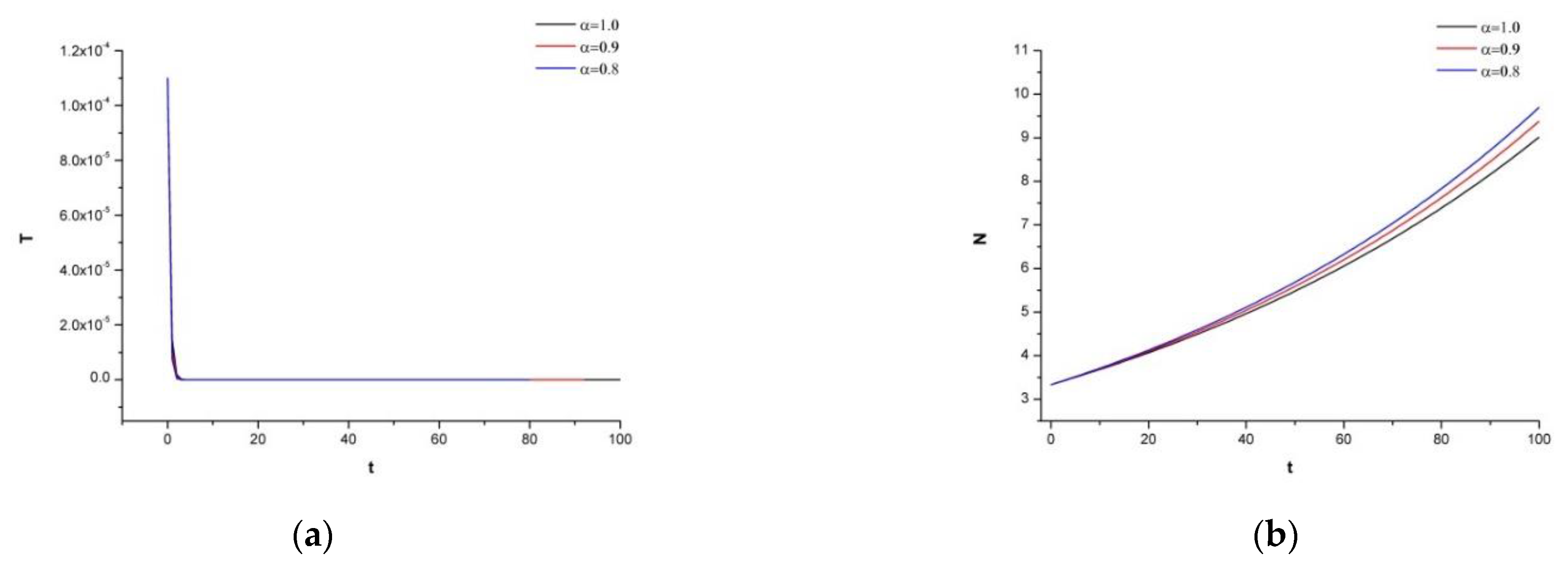
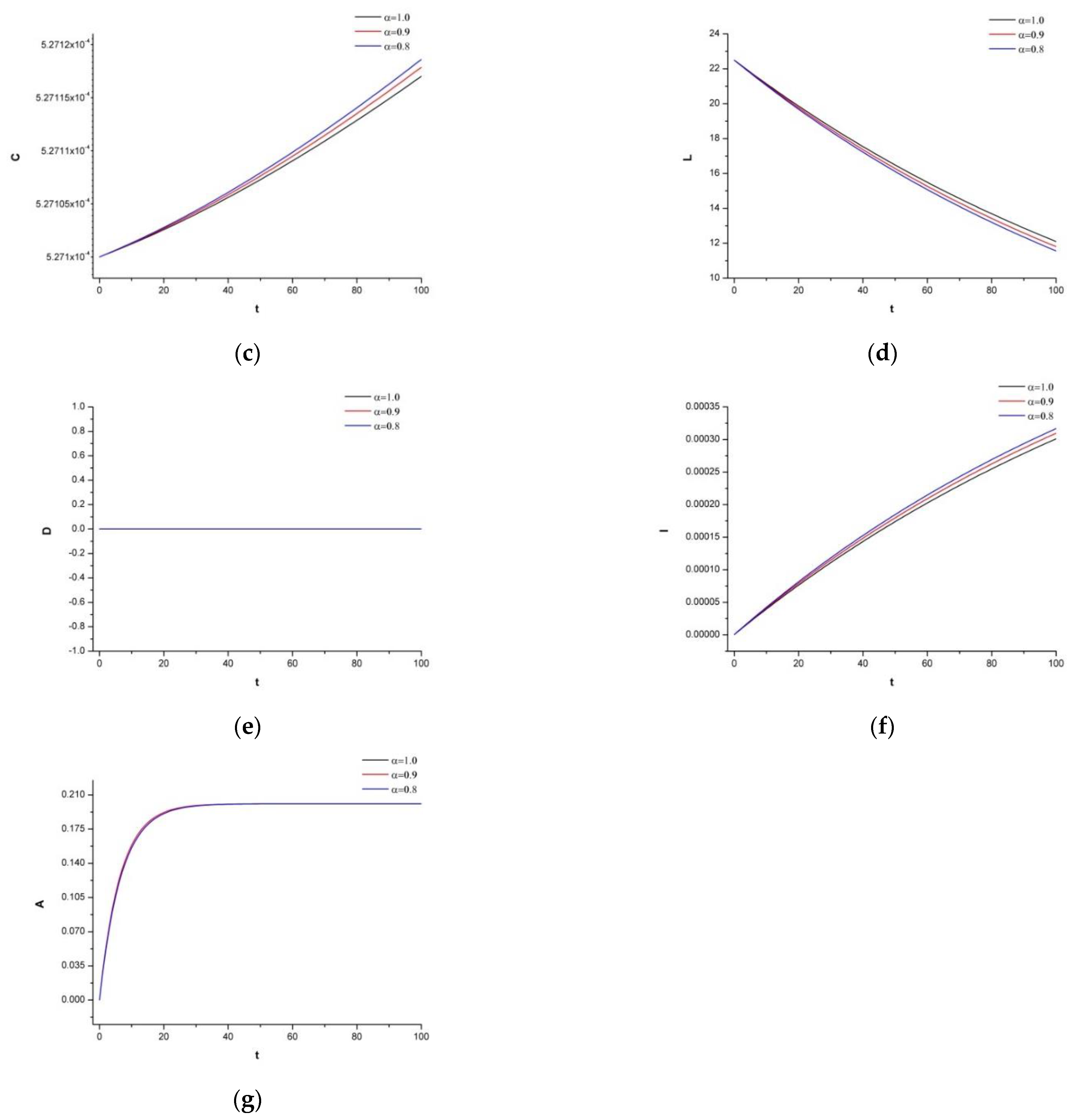
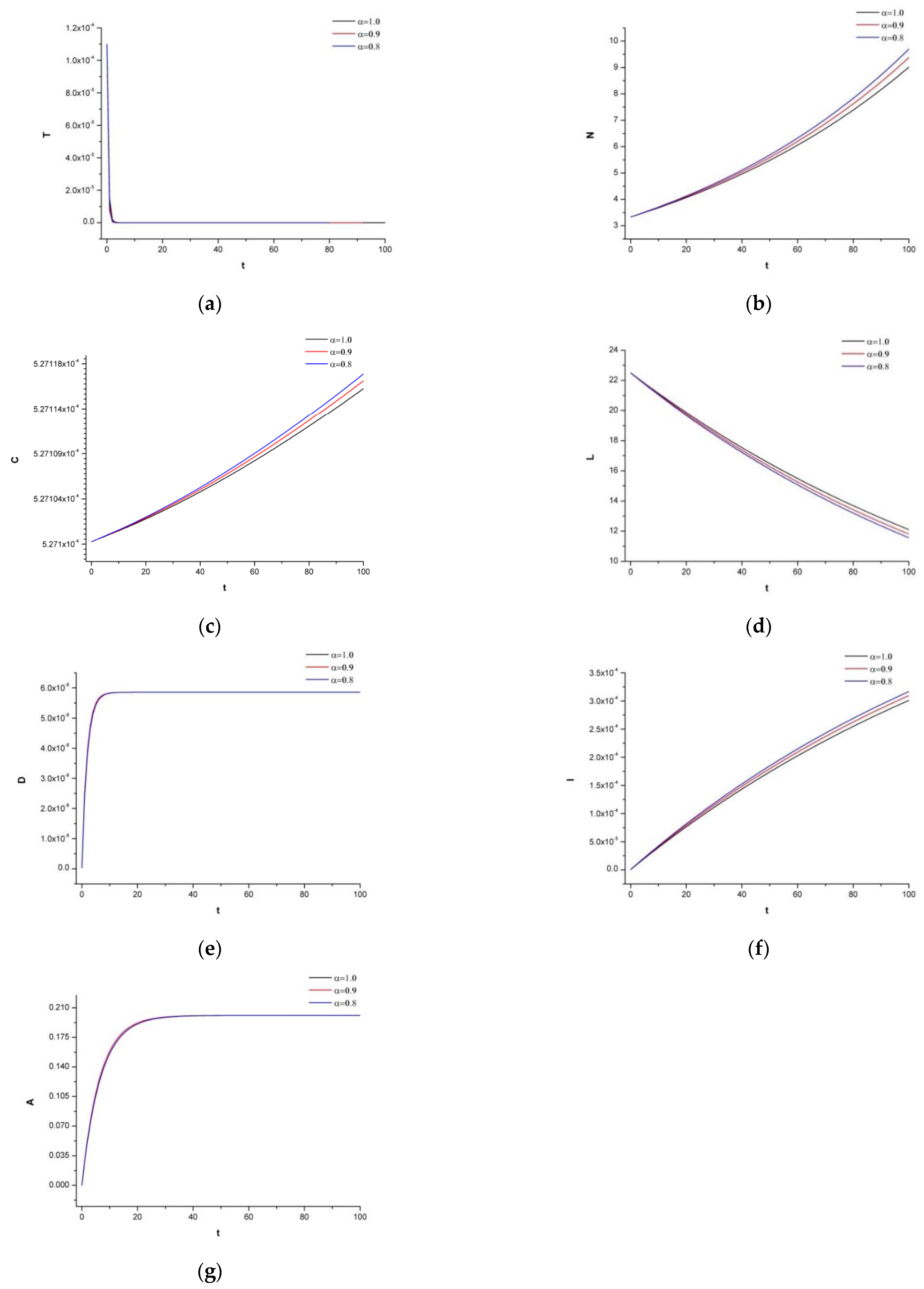
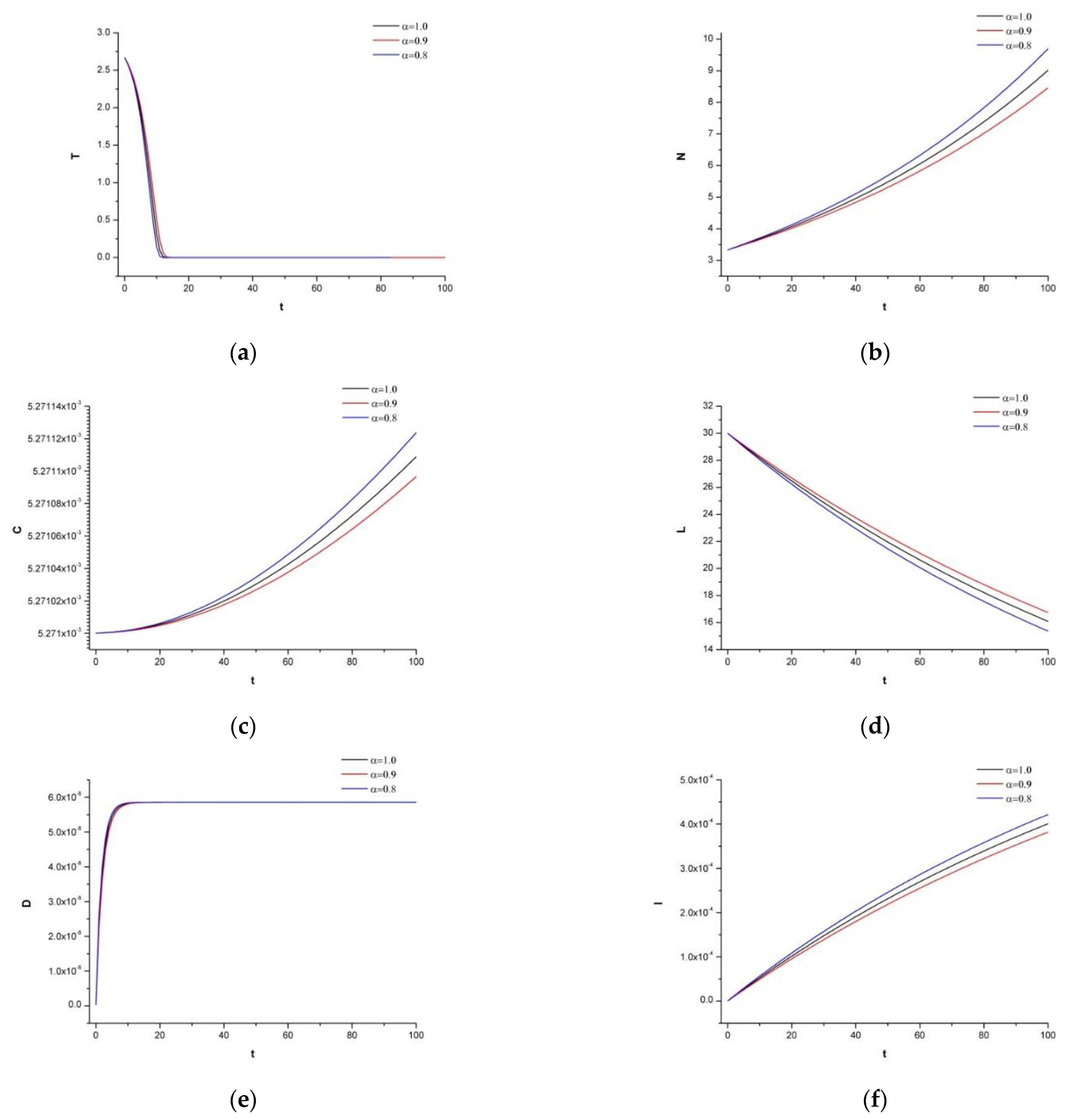
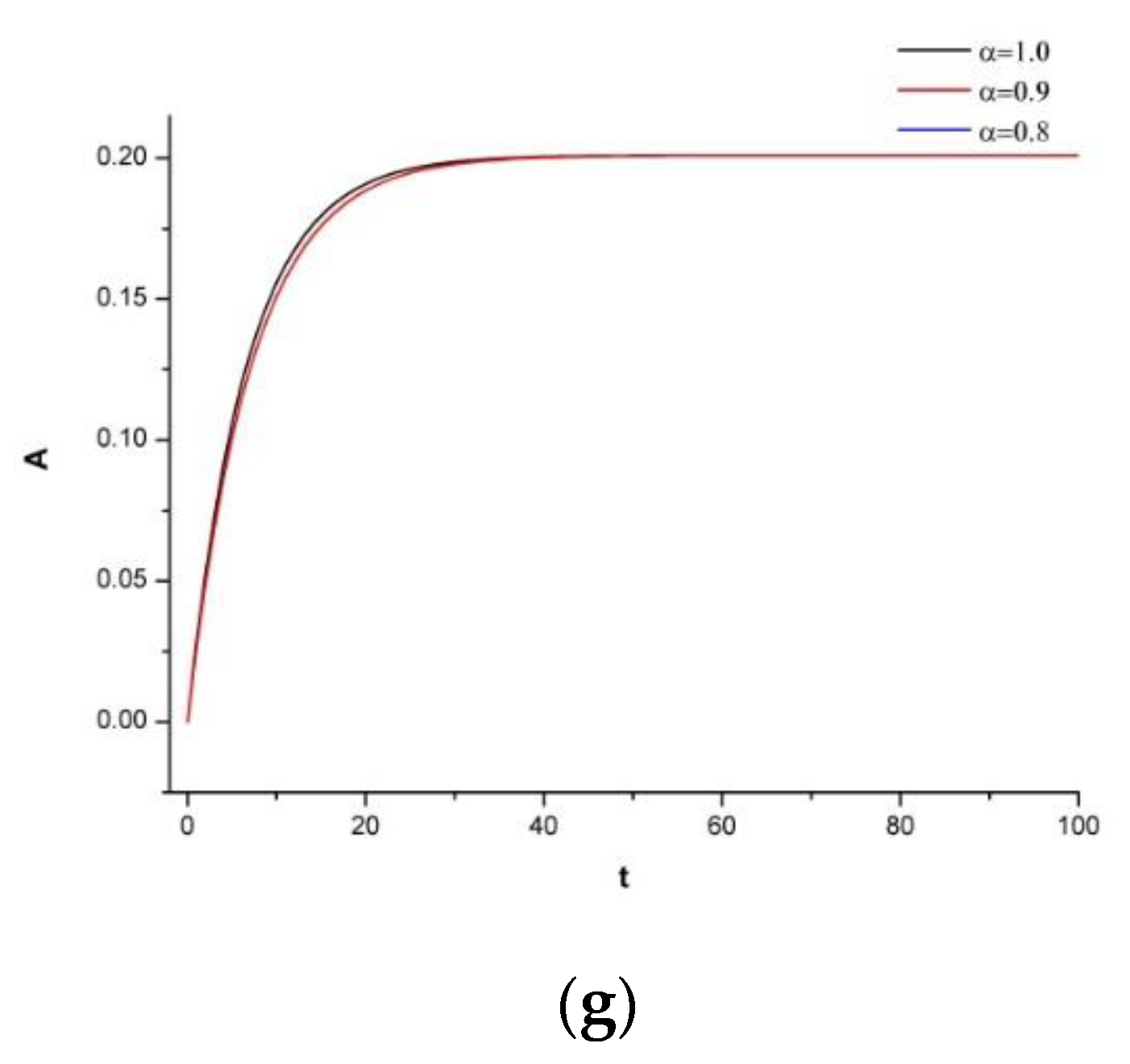
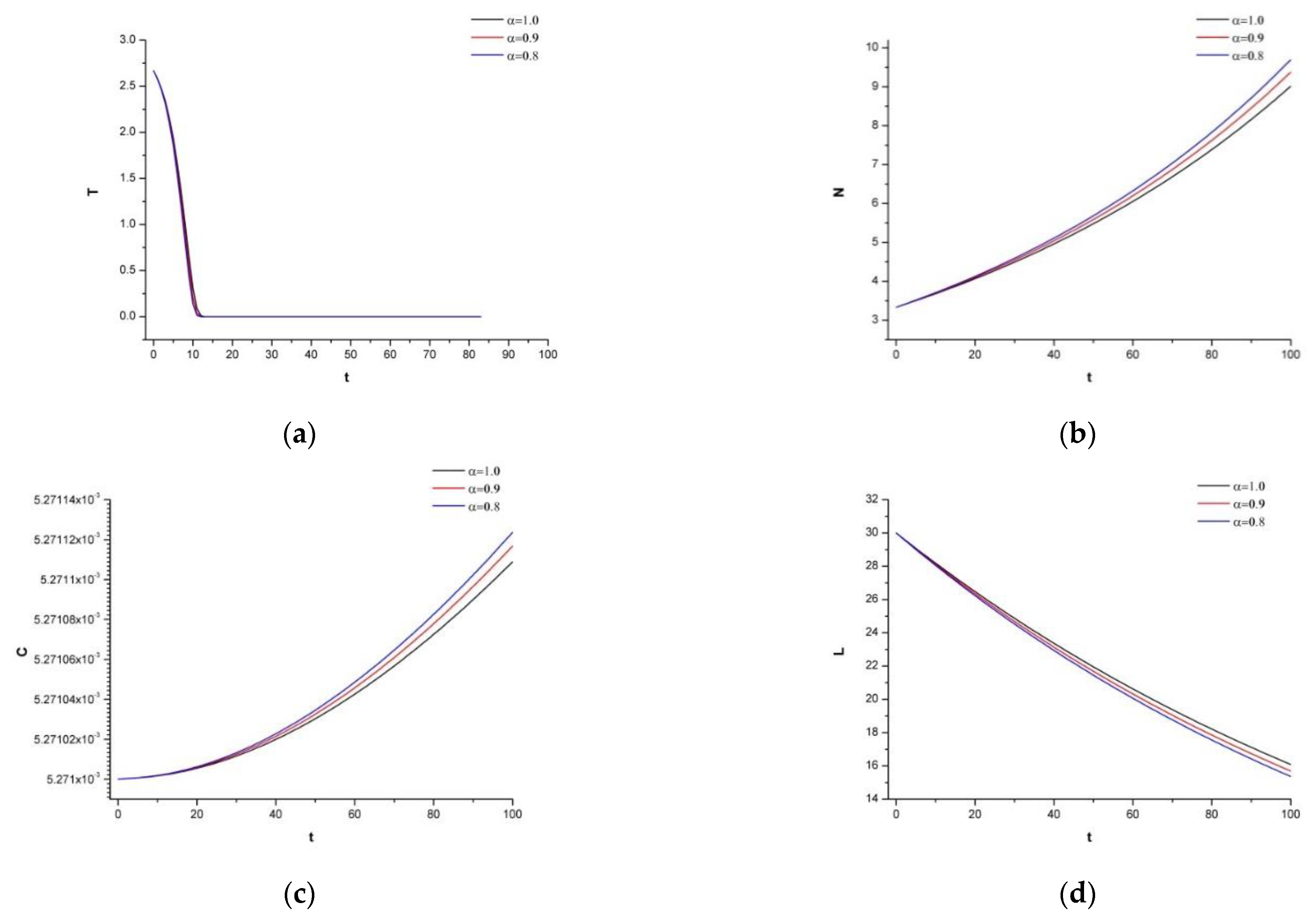
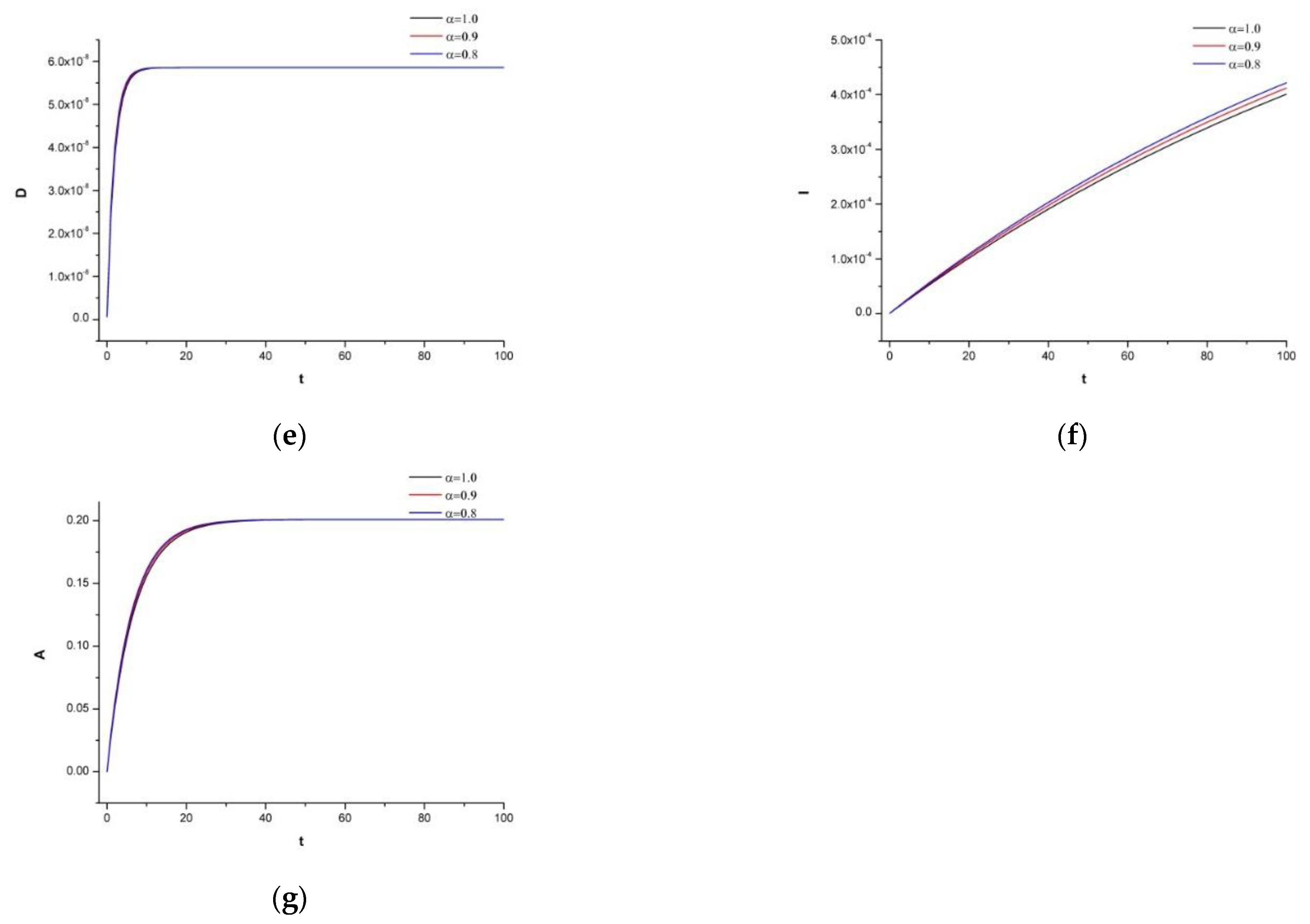
5. Simulation Results

We simulate the IVP (1) and (2) using the data obtained in

Table 2. Parametric values.

Notation	Value	References
$r$	$2.31\times {10}^{-1}$	[35]
${\alpha }_1$	$2.146\times {10}^{-10}$	[36]
${\beta }_1$	$5.156\times {10}^{-14}$	[2]
${\gamma }_1$	$0-8.1\times {10}^{-1}$	[37]
$\delta$	$0-3.125\times {10}^{-2}$	[38]
${\theta }_1$	[1.3–2.1]	[2]
${\omega }_1$	$[4\times {10}^{-3}-3\times {10}^{-2}]$	[2]
${\mu }_1$	$6.5\times {10}^{-10}$	[39]
${\epsilon }_1$	$1.25\times {10}^{-6}$	[39]
${\Lambda }_1$	$0.3$	[2]
$\rho$	$1\times {10}^{-2}$	[2]
${\alpha }_2$	$1.146\times {10}^{-10}$	theoretical finding
$\tau$	$5.13\times {10}^{-2}$	[2]
${\omega }_2$	$2.5036\times {10}^5$	[2]
${\mu }_2$	$6.5\times {10}^{-10}$	[39]
${\epsilon }_1$	$1.25\times {10}^{-6}$	[39]
${\beta }_2$	$5.156\times {10}^{-14}$	[2]
${\gamma }_2$	$9.048\times {10}^{-1}$	[40]
${\sigma }_1$	$5.156\times {10}^{-12}$	[2]
${\sigma }_2$	$1\times {10}^{-15}$	[2]
${\theta }_2$	$2.4036$	[2]
${\omega }_3$	$2.5036\times {10}^3$	[2]
$\xi$	$3.1718\times {10}^{-14}$	[2]
$\varrho$	$2.5036\times {10}^3$	[2]
${\beta }_3$	$5.156\times {10}^{-17}$	[2]
${\gamma }_3$	$4.524\times {10}^{-1}$	[40]
${\Lambda }_2$	$1.89\times {10}^5$	[2]
${\alpha }_3$	$6.3\times {10}^{-3}$	[2]
${\gamma }_4$	$5.7\times {10}^{-1}$	[40]
${\Lambda }_3$	$2.3869$	[2]
${\alpha }_4$	$4.077\times {10}^{-1}$	[40]
${\Lambda }_4$	$1.788\times {10}^{-7}$	[2]
${\alpha }_5$	$11.7427$	[2]
${\theta }_3$	$7.88\times {10}^{-2}$	[2]
${\omega }_4$	$2.5036\times {10}^3$	[2]
${\Lambda }_5$	$2.7859\times {10}^6$	[2]
${\alpha }_6$	$1.386\times {10}^{-1}$	[2]
${\mu }_3$	$8.9\times {10}^{-14}$	[41]
${\epsilon }_2$	$4.45\times {10}^{-5}$	[41]

. The developed model consists of tumor cells, components of the host’s immune response, and therapies such as irinotecan and Cetuximab, a monoclonal antibody concentration that has been FDA-approved for the treatment of colorectal cancer and is designed to bind to particular proteins. The literature for the study, which includes both in vivo and in vitro research on colorectal cancer, is thoroughly examined. It is seen that Cetuximab was applied with and without irinotecan to therapies to raise the survival rate and the condition of life [34].

We use the constructed model to explore the expected responses of the therapy for specific tumor cell populations. According to body mass, the person is a male who weighs 77 kg and has a chronic illness that has to be supported with additional nutrients to maintain a healthy immune system.

According to Table 2, the parameter values were obtained from in vivo and in vitro studies.

As a result, we first simulated the case of a disease-free equilibrium point, which can be assumed in the early detection of tumor density. In (I-a), we consider the treatment without irinotecan, and in (I-b), we add 30 $\mathrm{m}\mathrm{g}/{\mathrm{m}}^2$ once every 21 days. To see the simulation results more precisely, we multiplied the initial conditions by ${10}^{-8}$.

• (I-a)
  $$T\left(0\right)=1.1\times {10}^{-4},N\left(0\right)=3.333,C\left(0\right)=2.271\times {10}^{-4},L\left(0\right)=3\times {10}^1,D\left(0\right)=0,$$

  $$I\left(0\right)=4.892\times {10}^{-7},A\left(0\right)=2.5\times {10}^{-9},$$

  where we avoid the chemotherapy effect,
• (I-b)
  $$T\left(0\right)=1.1\times {10}^{-4},N\left(0\right)=3.333,C\left(0\right)=2.271\times {10}^{-4},L\left(0\right)=3\times {10}^1,$$

  $$D\left(0\right)=3\times {10}^{-10},I\left(0\right)=4.892\times {10}^{-7},A\left(0\right)=2.5\times {10}^{-9},$$

  where the effect of irinotecan is included.

For this scenario, the clinical data showed extinction of the tumor density for cases (I-a) and (I-b).

As analyzing the stability of a coexisting equilibrium point implies that the tumor has already attained a significant density, we make the following assumption with the following initial condition:

• (II-a)
  $$T\left(0\right)=2.67\times {10}^{-1},N\left(0\right)=3.333\times {10}^8,C\left(0\right)=5.2671\times {10}^{-3},L\left(0\right)=3\times {10}^1,$$

  $$D\left(0\right)=0,I\left(0\right)=4.892\times {10}^{-7},A\left(0\right)=4\times {10}^{-9},$$

  where we focus on the immunotherapy and mAb,
• (II-b)
  $$T\left(0\right)=2.67\times {10}^{-1},N\left(0\right)=3.333,C\left(0\right)=5.2671\times {10}^{-3},L\left(0\right)=3\times {10}^1,$$

  $$D\left(0\right)=3\times {10}^{-10},I\left(0\right)=4.892\times {10}^{-7},A\left(0\right)=4\times {10}^{-9},$$

  where all treatment supplements (including irinotecan) are involved.
• (II-c)
  $$T\left(0\right)=2.67\times {10}^{-1},N\left(0\right)=3.333,C\left(0\right)=5.2671\times {10}^{-3},L\left(0\right)=3\times {10}^1,$$

  $$D\left(0\right)=6\times {10}^{-10},I\left(0\right)=4.892\times {10}^{-7},A\left(0\right)=4\times {10}^{-9},$$

  where all treatment supplements (including irinotecan) are involved.

In this scenario, the clinical data illustrate an increase in the tumor density for (II-a), meaning that IL-2 treatment and the concentration of Cetuximab were insufficient to control the growth of the tumor cell population. Case (II-b) showed that growth decreases if all treatment supplements are involved in the therapy. By increasing the dosage of the chemotherapeutic drug to 60 $\mathrm{m}\mathrm{g}/{\mathrm{m}}^2$ once every 21 days, the tumor cell population is rendered extinct.

Figure 1 illustrates the graph of system (1) for each compartment with the initial conditions given in (I-a). The tumor cell population is low and represents an early detected case of colorectal cancer. Considering now the in vivo and in vitro studies of [5,34], it is emphasized that the $IL-2$ concentration and the mAb drug of Cetuximab would be sufficient for the treatment to shrink the tumor density.

For system (1) and the initial conditions in (I-a), it is seen that the tumor density is extinct. There is no need to provide irinotecan with this appropriate therapy because it already reaches every region of the body through the bloodstream; this indicates that $D\left(0\right)=0$.

Figure 2 shows the graph of system (1) with the initial conditions of (I-b). In this example, irinotecan is included in the treatment, and a similar result to (I-a) is obtained. Figure 2 is a vital graph emphasizing that not all mixed therapies should include chemotherapy. In the case of both (I-a) and (I-b), the tumor density decreases, while in (I-b), one should notice that the chemotherapeutic drug also destroys normal tissues and affects the immune system. Therefore, considering the whole dynamic of the system, it is notable to support the body with additional supplements that keep the immune system strong instead of increasing the variation of the drugs.

When the tumor has already achieved a certain density, as in Figure 3, only the IL-2 concentration can assist the immune system, and the dosage of mAb is insufficient. The tumor has a cell population of $T\left(0\right)=1.4\times {10}^7.$ While the tumor density expanded quickly, we also noticed that the natural killers were interacting heavily.

To observe the system’s dynamic response, we now add 30 mg of irinotecan under the identical supposition as in Figure 3. Figure 4 represents the immune-chemotherapeutic treatment with the monoclonal antibody cetuximab and a successful result of a decrease in the tumor compartment. Since the aim is to keep the immune system strong and to avoid any destruction of the normal tissue, we believe, as is also mentioned in the references of Table 2, that for this tumor density, the dosage is enough to reach the desired outcome.

In addition, we want to increase the dosage of the chemotherapeutic drug to $D\left(0\right)=0.06$ to show the side effect on the human body.

As expected, we see in Figure 5 that the normal cells are also affected by the drug, which destroys the immune system. Thus, the patient can be attacked by any other chronic or non-chronic disease, which would lead to unexpected results.

6. Conclusions

Fractional calculus is an extension of traditional calculus because derivatives and integrals are defined for any real order. In some cases, fractional operators are superior to traditional derivatives and integrals for representing systems with high-order dynamics and complex nonlinear processes.

To describe the dynamical behavior of colorectal cancer following immune chemotherapy with mAb-Cetuximab, we proposed a system of fractional order differential equations. The study’s goal is to investigate and present the efficacy of various immune system-supporting supplements and the way that cancer tissues react to monoclonal antibody therapy (mAb). The combined therapy focuses on eliminating the cancerous tissues and boosting the immune system with supplements rather than putting the patient through a painful and drawn-out treatment. Thus, in Section 2 we defined the system with seven compartments: $T\left(t\right),$ colorectal cancer cells; $N\left(t\right),$ compartment of natural killer (N.K.); $C\left(t\right),$ the CD$8^{+}$T-cell population; $L\left(t\right),$ the lymphocytes population; $D\left(t\right),$ the irinotecan concentration; $I\left(t\right),$ the IL-2 concentration; $A\left(t\right)$, the mAb Cetuximab concentration.

The local stability of the disease-free and co-existing equilibrium points was theoretically demonstrated in Section 3. Section 4 showed the condition of global stability, where discretization processes were applied to analyze the discrete treatment in an expanded interval. We proved theoretically and numerically how important it is to apply both immunotherapy and mAb treatment in order to prevent the negative effects of chemotherapeutic medications based on the early diagnosis of the tumor and the significant density of the cancer cells. Furthermore, it is emphasized that the need for irinotecan is essential in further stages of tumor density. The amount of this prescription (irinotecan), however, has a damaging power to natural killers, which affects the human body’s immune system—particularly when the person has a chronic illness and needs intense immune system support. As a result, the timing should be carefully planned, taking into account the ideal concentration required to reduce the tumor density.

In Section 5, we provided several early detection and tumor density stage scenarios to demonstrate the findings. We observed that different treatment approaches are required given the tumor density and the immune system’s supplementation requirements. As a result, it is seen that alternative treatment strategies have to be applied in considering the density of the tumor and the necessity of optimal dosage in the therapy.

References

1. World Cancer Research Fund International. 2020. Available online: https://www.wcrf.org/cancer-trends/worldwide-cancer-data/ (accessed on 1 January 2023).
2. de Pillis, L.; Fister, K.R.; Gu, W.; Collins, C.; Daub, M.; Gross, D.; Moore, J.; Preskill, B. Mathematical Model Creation for Cancer Chemo-Immunotherapy. Comput. Math. Methods Med. 2009, 10, 165–184. [Google Scholar] [CrossRef]
3. Abbas, A.K.; Lichtman, A.H. Cellular and Molecular Immunology, 5th ed.; Elsevier: St. Louis, MO, USA, 2005. [Google Scholar]
4. Kirschner, D.; Jackson, T.; Arciero, J. A mathematical model of tumor-immune evasion and siRNA treatment. Discret. Contin. Dyn. Syst. B 2003, 4, 39–58. [Google Scholar] [CrossRef]
5. Depillis, L.; Savage, H.; Radunskaya, A. Mathematical Model of Colorectal Cancer with Monoclonal Antibody Treatments. Br. J. Med. Med. Res. 2014, 4, 3101–3131. [Google Scholar] [CrossRef] [PubMed]
6. Chaplain, M.; Matzavinos, A. Mathematical modeling of spatio-temporal phenomena in tumor immunology. Tutor. Math. Biosci. III 2006, 1872, 131–183. [Google Scholar] [CrossRef]
7. De Boer, R.J.; Mohri, H.; Ho, D.D.; Perelson, A.S. Turnover Rates of B Cells, T Cells, and NK Cells in Simian Immunodeficiency Virus-Infected and Uninfected Rhesus Macaques. J. Immunol. 2003, 170, 2479–2487. [Google Scholar] [CrossRef]
8. Nelson, B.H. IL-2, Regulatory T Cells, and Tolerance. J. Immunol. 2004, 172, 3983–3988. [Google Scholar] [CrossRef]
9. Asquith, B.; Debacq, C.; Florins, A.; Gillet, N.; Sanchez-Alcaraz, T.; Mosley, A.; Willems, L. Quantifying lymphocyte kinetics in vivo using carboxyfluorescein diacetate succinimidyl ester. Proc. R. Soc. B Boil. Sci. 2006, 273, 1165–1171. [Google Scholar] [CrossRef]
10. Kirschner, D.; Panetta, J.C. Modeling immunotherapy of the tumor—Immune interaction. J. Math. Biol. 1998, 37, 235–252. [Google Scholar] [CrossRef]
11. Gültürk, I.; Erdal, G.; Özmen, A.; Tacar, S.Y.; Yilmaz, M.; Tural, D. With metastatic colorectal cancer: A single center experience use of monoclonal antibodies (Bevacizumab, Cetuximab, and Panitumumab) in patients. J. Exp. Clin. Med. 2022, 39, 1112–1119. [Google Scholar] [CrossRef]
12. de Pillis, L.; Gu, W.; Radunskaya, A. Mixed immunotherapy and chemotherapy of tumors: Modeling, applications and biological interpretations. J. Theor. Biol. 2006, 238, 841–862. [Google Scholar] [CrossRef]
13. Al-Khaled, K.; Alquran, M. An approximate solution for a fractional model of generalized Harry Dym equation. Math. Sci. 2014, 8, 125–130. [Google Scholar] [CrossRef]
14. Yousef, A.; Yousef, F.B. Bifurcation and Stability Analysis of a System of Fractional-Order Differential Equations for a Plant–Herbivore Model with Allee Effect. Mathematics 2019, 7, 454. [Google Scholar] [CrossRef]
15. Bozkurt, F.; Yousef, A.; Abdeljawad, T. Analysis of the outbreak of the novel coronavirus COVID-19 dynamic model with control mechanisms. Results Phys. 2020, 19, 103586. [Google Scholar] [CrossRef] [PubMed]
16. Almeida, R.; Bastos, N.R.O.; Monteiro, M.T.T. Modeling some real phenomena by fractional differential equations. Math. Methods Appl. Sci. 2015, 39, 4846–4855. [Google Scholar] [CrossRef]
17. Zhang, T.; Qian, Y. Stability analysis of several first order schemes for the Oldroyd model with smooth and nonsmooth initial data. Numer. Methods Partial. Differ. Equ. 2018, 34, 2180–2216. [Google Scholar] [CrossRef]
18. Mustafa, O. Effect of nonlocal transformations on the linearizability and exact solvability of the nonlinear generalized modified Emden-type equations. Int. J. Geom. Methods Mod. Phys. 2022, 19, 2250158. [Google Scholar] [CrossRef]
19. Özdemir, N.; Uçar, E. Investigating of an immune system-cancer mathematical model with Mittag-Leffler kernel. AIMS Math. 2020, 5, 1519–1531. [Google Scholar] [CrossRef]
20. Ahmad, W.M.; Sprott, J. Chaos in fractional-order autonomous nonlinear systems. Chaos Solitons Fractals 2003, 16, 339–351. [Google Scholar] [CrossRef]
21. Yousef, A.; Bozkurt, F.; Abdeljawad, T. Qualitative Analysis of a Fractional Pandemic Spread Model of the Novel Coronavirus (COVID-19). Comput. Mater. Contin. 2020, 66, 843–869. [Google Scholar] [CrossRef]
22. Bagley, R.L.; Calico, R.A. Fractional order state equations for the control of viscoelasticallydamped structures. J. Guid. Control Dyn. 1991, 14, 304–311. [Google Scholar] [CrossRef]
23. Ahmed, E.; El-Sayed, A.; El-Saka, H.A. On some Routh–Hurwitz conditions for fractional order differential equations and their applications in Lorenz, Rössler, Chua and Chen systems. Phys. Lett. A 2006, 358, 1–4. [Google Scholar] [CrossRef]
24. Li, L.; Liu, J.-G. A Generalized Definition of Caputo Derivatives and Its Application to Fractional ODEs. SIAM J. Math. Anal. 2018, 50, 2867–2900. [Google Scholar] [CrossRef]
25. Kilbas, A.A.; Srivastava, H.M.; Trujillo, J.J. Theory and Applications of Fractional Differential Equations; Elsevier: Amsterdam, The Netherlands, 2006; Volume 204. [Google Scholar]
26. Kuznetsov, V.; Makalkin, I.; Taylor, M.; Perelson, A. Nonlinear dynamics of immunogenic tumors: Parameter estimation and global bifurcation analysis. Bull. Math. Biol. 1994, 56, 295–321. [Google Scholar] [CrossRef] [PubMed]
27. Dunne, J.; Lynch, S.; O’farrelly, C.; Todryk, S.; Hegarty, J.E.; Feighery, C.; Doherty, D.G. Selective Expansion and Partial Activation of Human NK Cells and NK Receptor-Positive T Cells by IL-2 and IL-15. J. Immunol. 2001, 167, 3129–3138. [Google Scholar] [CrossRef] [PubMed]
28. Orditura, M.; Romano, C.; De Vita, F.; Galizia, G.; Lieto, E.; Infusino, S.; De Cataldis, G.; Catalano, G. Behaviour of interleukin-2 serum levels in advanced non-small-cell lung cancer patients: Relationship with response to therapy and survival. Cancer Immunol. Immunother. 2000, 49, 530–536. [Google Scholar] [CrossRef] [PubMed]
29. Odibat, Z.M.; Shawagfeh, N.T. Generalized Taylor’s formula. Appl. Math. Comput. 2007, 186, 286–293. [Google Scholar] [CrossRef]
30. Owusu-Mensah, I.; Akinyemi, L.; Oduro, B.; Iyiola, O.S. A fractional order approach to modeling and simulations of the novel COVID-19. Adv. Differ. Equ. 2020, 2020, 683. [Google Scholar] [CrossRef]
31. Özalp, N.; Demirci, E. A fractional order SEIR model with vertical transmission. Math. Comput. Model. 2011, 54, 1–6. [Google Scholar] [CrossRef]
32. Matignon, D. Stability results for fractional-order differential equations with applications to control processing. Comput. Eng. Sys. Appl. 1996, 2, 963–968. [Google Scholar]
33. Zeng, Q.S.; Cao, G.Y.; Zhu, X.J. The asymptotic stability on sequential fractional-order systems. J. Shanghai Jiaotong Univ. 2005, 39, 346–348. [Google Scholar]
34. Martinelli, E.; De Palma, R.; Orditura, M.; De Vita, F.; Ciardiello, F. Anti-epidermal growth factor receptor monoclonal antibodies in cancer therapy. Clin. Exp. Immunol. 2009, 158, 1–9. [Google Scholar] [CrossRef] [PubMed]
35. Corbett, T.H.; Griswold Jr, D.P.; Roberts, B.J.; Peckham, J.C.; Schabel, F.M., Jr. Tumor induction relationships in development of transplantable cancers of the colon in mice for chemotherapy assays, with a note on carcinogen structure. Cancer Res. 1975, 35, 2434–2439. Available online: https://pubmed.ncbi.nlm.nih.gov/1149045/ (accessed on 1 January 2023). [PubMed]
36. Leith, J.T.; Michelson, S.; Faulkner, L.E.; Bliven, S.F. Growth properties of artificial heterogeneous human colon tumors. Cancer Res. 1987, 47, 1045–1051. Available online: https://pubmed.ncbi.nlm.nih.gov/3802089/ (accessed on 1 January 2023).
37. Vilar, E.; Scaltriti, M.; Balmaña, J.; Saura, C.; Guzmán, M.; Arribas, J.; Baselga, J.; Tabernero, J. Microsatellite instability due to hMLH1 deficiency is associated with increased cytotoxicity to irinotecan in human colorectal cancer cell lines. Br. J. Cancer 2008, 99, 1607–1612. [Google Scholar] [CrossRef] [PubMed]
38. De Vita, V., Jr.; Hellman, S.; Rosenberg, S. Cancer: Principles and Practice of Oncology, 7th ed.; Lippincott Wiliams & Wilkins: Philadelphia, PA, USA, 2000. [Google Scholar]
39. Kurai, J.; Chikumi, H.; Hashimoto, K.; Yamaguchi, K.; Yamasaki, A.; Sako, T.; Touge, H.; Makino, H.; Takata, M.; Miyata, M.; et al. Antibody-Dependent Cellular Cytotoxicity Mediated by Cetuximab against Lung Cancer Cell Lines. Clin. Cancer Res. 2007, 13, 1552–1561. [Google Scholar] [CrossRef] [PubMed]
40. Catimel, G.; Chabot, G.G.; Guastalla, J.P.; Dumortier, A.; Cote, C.; Engel, C.; Gouyette, A.; Mathieu-Boué, A.; Mahjoubi, M.; Clavel, M. Phase I and pharmacokinetic study of irinotecan (CPT-11) administered daily for three consecutive days every three weeks in patients with advanced solid tumors. Ann. Oncol. 1995, 6, 133–140. [Google Scholar] [CrossRef] [PubMed]
41. Freeman, D.; Sun, J.; Bass, R.; Jung, K.; Ogbagabriel, S.; Elliott, G.; Radinsky, R. Panitumumab and cetuximab epitope mapping and in vitro activity. J. Clin. Oncol. 2008, 26, 14536. [Google Scholar] [CrossRef]
Figure 1. (a) Dynamics of the tumor density for T 0 = 1.1 × 10 4 , (b) Dynamics of N.K. for N 0 = 3.333 , (c) Dynamics of CD 8 + T-cell for C 0 = 2.271 × 10 4 , (d) Dynamics of lymphocytes for L 0 = 3 × 10 1 , (e) Dynamics of irinotecan for D ( 0 ) = 0 , (f) Dynamics of IL-2 for I 0 = 4.892 × 10 7 , (g) Dynamics of Cetuximab for A 0 = 2.5 × 10 9 .
Mathematics 11 02374 g001aMathematics 11 02374 g001b
Figure 2. (a) Dynamics of the tumor density for T 0 = 1.1 × 10 4 , (b) Dynamics of N.K. for N 0 = 3.333 , (c) Dynamics of CD 8 + T-cell for C 0 = 2.271 × 10 4 , (d) Dynamics of lymphocytes for L 0 = 3 × 10 1 , (e) Dynamics of irinotecan for D ( 0 ) = 3 × 10 10 , (f) Dynamics of IL-2 for I 0 = 4.892 × 10 7 , (g) Dynamics of Cetuximab for A 0 = 2.5 × 10 9 .
Mathematics 11 02374 g002
Figure 3. (a) Dynamics of the tumor density for T 0 = 2.67 × 10 1 , (b) Dynamics of N.K. for N 0 = 3.333 , (c) Dynamics of CD 8 + T-cell for C 0 = 5.2671 × 10 3 , (d) Dynamics of lymphocytes for L 0 = 3 × 10 1 L , (e) Dynamics of irinotecan for D ( 0 ) = 0 , (f) Dynamics of IL-2 for I 0 = 4.892 × 10 7 , (g) Dynamics of Cetuximab for A 0 = 4 × 10 9 .
Mathematics 11 02374 g003
Figure 4. (a) Dynamics of tumor density for T 0 = 2.67 × 10 1 , (b) Dynamics of N.K. for N 0 = 3.333 , (c) Dynamics of CD 8 + T-cell concentration for C 0 = 5.2671 × 10 3 , (d) Dynamics of lymphocytes for L 0 = 3 × 10 1 , (e) Dynamics of irinotecan for D ( 0 ) = 3 × 10 10 , (f) Dynamics of IL-2 for I 0 = 4.892 × 10 7 , (g) Dynamics of Cetuximab for A 0 = 4 × 10 9 .
Mathematics 11 02374 g004aMathematics 11 02374 g004b
Figure 5. (a) Dynamics of tumor density for T 0 = 2.67 × 10 1 , (b) Dynamics of N.K. for N 0 = 3.333 , (c) Dynamics of CD 8 + T-cell concentration for C 0 = 5.2671 × 10 3 , (d) Dynamics of lymphocytes for L 0 = 3 × 10 1 , (e) Dynamics irinotecan for D ( 0 ) = 6 × 10 10 , (f) Dynamics of IL-2 for I 0 = 4.892 × 10 7 , (g) Dynamics of Cetuximab for A 0 = 4 × 10 9 .
Mathematics 11 02374 g005aMathematics 11 02374 g005b