

A Proposed Analytical and Numerical Treatment for the Nonlinear SIR Model via a Hybrid Approach

Department of Mathematics, College of Science, Majmaah University, Al-Majmaah 11952, Saudi Arabia
Mathematics 2023, 11(12), 2749; https://doi.org/10.3390/math11122749
Submission received: 14 May 2023
/
Revised: 9 June 2023
/
Accepted: 13 June 2023
/
Published: 17 June 2023
(This article belongs to the Special Issue Computational Mathematics and Mathematical Modelling)
Abstract
:This paper re-analyzes the nonlinear Susceptible–Infected–Recovered (SIR) model using a hybrid approach based on the Laplace–Padé technique. The proposed approach is successfully applied to extract several analytic approximations for the infected and recovered individuals. The domains of applicability of such analytic approximations are addressed. In addition, the present results are validated through various comparisons with the Runge–Kutta numerical method. The obtained analytical results agree with the numerical ones for a wide range of numbers of contacts featured in the studied model. The efficiency of the present analysis reveals that it can be implemented to deal with other systems describing real-life phenomena.
Keywords:
Laplace; Padé; ordinary differential equation; initial value problem; series solution; exact solutionMSC:
34A34; 34A451. Introduction
Mathematical models of real-life phenomena are often governed by ordinary differential equations (ODEs) or partial differential equations (PDEs). Searching for analytical or numerical solutions for such models requires accurate methods, whether analytical or numerical, for the better interpretation of the involved phenomena. In this context, mathematicians have invented and developed many ways to solve mathematical and physical models. For example, the Adomian decomposition method (ADM) [1,2,3,4,5,6,7,8,9,10,11] is one of the most popular methods which has been widely used during recent decades; the same applies to the homotopy perturbation method (HPM) [12,13,14,15], the homotopy analysis method (HAM) [16,17], and the differential transform method (DTM) [18,19,20,21]. However, each of these methods has its own advantages, but at the same time has some defects that must be faced and overcome. Although the above-mentioned methods were found effective in solving a considerable number of mathematical/physical models, a massive amount of computational work is sometimes needed to reach the desired accuracy. The major step when applying the ADM is to calculate the Adomian polynomials of the involved nonlinear terms, while the HPM requires an effective canonical form for the equation/system being solved in addition to imposing an auxiliary parameter. Moreover, one of the main difficulties of the HAM lies in the necessity of choosing an effective/accurate initial guess function, according to which the solution is constructed. Therefore, any unfavorable choice of such an initial guess function will give either an inaccurate or divergent solution.
In order to avoid all the aforementioned difficulties, we will present in this study an alternative approach that may be appropriate and direct to solve ODEs. The first step of the suggested approach is mainly based on obtaining a series solution of the governing equation and then deriving the Laplace transform (LT) of this series. The second step is to construct the Padé approximants of the transformed series and then apply the inverse LT as a final step to construct the approximate analytic solution. For this purpose, it is possible to construct different forms of Padé approximants, including diagonal and non-diagonal. Accordingly, different approximations can be constructed for the required analytic solution. The accuracy of our approach can be validated via performing comparisons with other trusted methods, whether analytical or numerical. In addition, the accuracy of the current method can be evaluated, independently, through calculating the residual errors resulting from the substitution of the obtained approximate analytic solution into the governing equation/system.
The nonlinear Susceptible–Infected–Recovered (SIR) model is considered in this paper as a test example. The SIR model has been employed in Refs. [22,23] to study the COVID-19 pandemic, which is still of interest to many researchers worldwide. The SIR model was first established in Ref. [22] by means of the following system of ODEs:
where and are the infected and the recovered individuals, respectively. represents the susceptible individuals, . The parameter describes the transmission rate, which is used to estimate the number of contacts between susceptible and infected individuals. The initial conditions (ICs) are
A summary of the paper is as follows. In Section 2, a power series solution (PSS) for the system (1)–(3) is derived. Section 3 focuses on applying the proposed approach through combining the LT and the Padé approximants. Furthermore, different analytical approximations for and are established in Section 3. Section 4 is devoted to validating the obtained results, where several comparisons with the Runge–Kutta method are conducted. Moreover, the domains of applicability of the current analysis are demonstrated and addressed in Section 4. In addition, the accuracy of our approach is explored and confirmed via residual errors. The paper is concluded in Section 5.
2. The Series Solution
The system of Equations (1) and (2) can be easily reduced to the following second-order nonlinear ODE:
under the ICs
Let us search for a power series solution (PSS) of Equations (4) and (5) in the form:
In view of (5) and (6), the terms and are A and B, respectively. Furthermore, we have
Substituting (6) and (7) into (4) implies
Using the initial terms and , the coefficients of the series can be generated and are given as
and so on. Employing the above coefficients in Equation (6), we obtain the following PSS for :
while the PSS for can be obtained through differentiating (6) once with respect to , which gives
i.e.,
where the terms of the preceding PSS may be increased as needed to ensure the desired accuracy. However, it will be shown later that the PSS has limitations regarding the domain of convergence. Such drawbacks can be overcome by the current approach which is the subject of the next section.
3. The Laplace–Padé Technique
3.1. Approximation for
Applying the Laplace transform (LT) to series (6) yields
Suppose that ; then,
Constructing Padé [1/1] for the last series gives
Reversing the last expression with respect to s, we obtain
The inversion of gives the approximation as
The Padé [1/2] for series (17) is
where
This expression transforms to the trigonometric form
when
From (17), we have the following expression for Padé [2/2] :
where
Based on (28), we have
which leads to
or equivalently,
Similarly, one can obtain
which can be inverted to give
where the quantities , and () are given by
and
Furthermore, , , and are three distinct roots of the cubic algebraic equation
Furthermore, we can calculate the diagonal Padé approximant as
which has the following inversion:
where the quantities , , and () are
and
while , are three distinct roots of the cubic equation
Remark 1.
It should be noted that the inversion of Equation (41) depends on the three roots of the denominator. To clarify this point, assume that , are three distinct roots of the denominator in (41), i.e., ; then, one can rewrite Equation (41) as
Using partial fractions, we can express as
where , are given by Equation (48). It is now clear that the inversion of in the last equation gives Formula (42).
3.2. Approximation for
Proceeding as above, one can obtain
and
The inversions of the above expressions give
and
where
The approximation can also be established using the same procedure. However, it will be shown later that is sufficient to achieve the desired accuracy.
4. Results and Validation
In this section, we focus on validating the accuracy of the current analysis. Various comparisons are performed to reveal the validity of the present PSS and the Padé approximants for the recovered and infected individuals and , respectively. The explicit Runge–Kutta method (ERKM) is chosen as a reference numerical method to explore the effectiveness and efficiency of our accuracy.
To achieve this task, we may express the j-term of the PSS for and , respectively, as
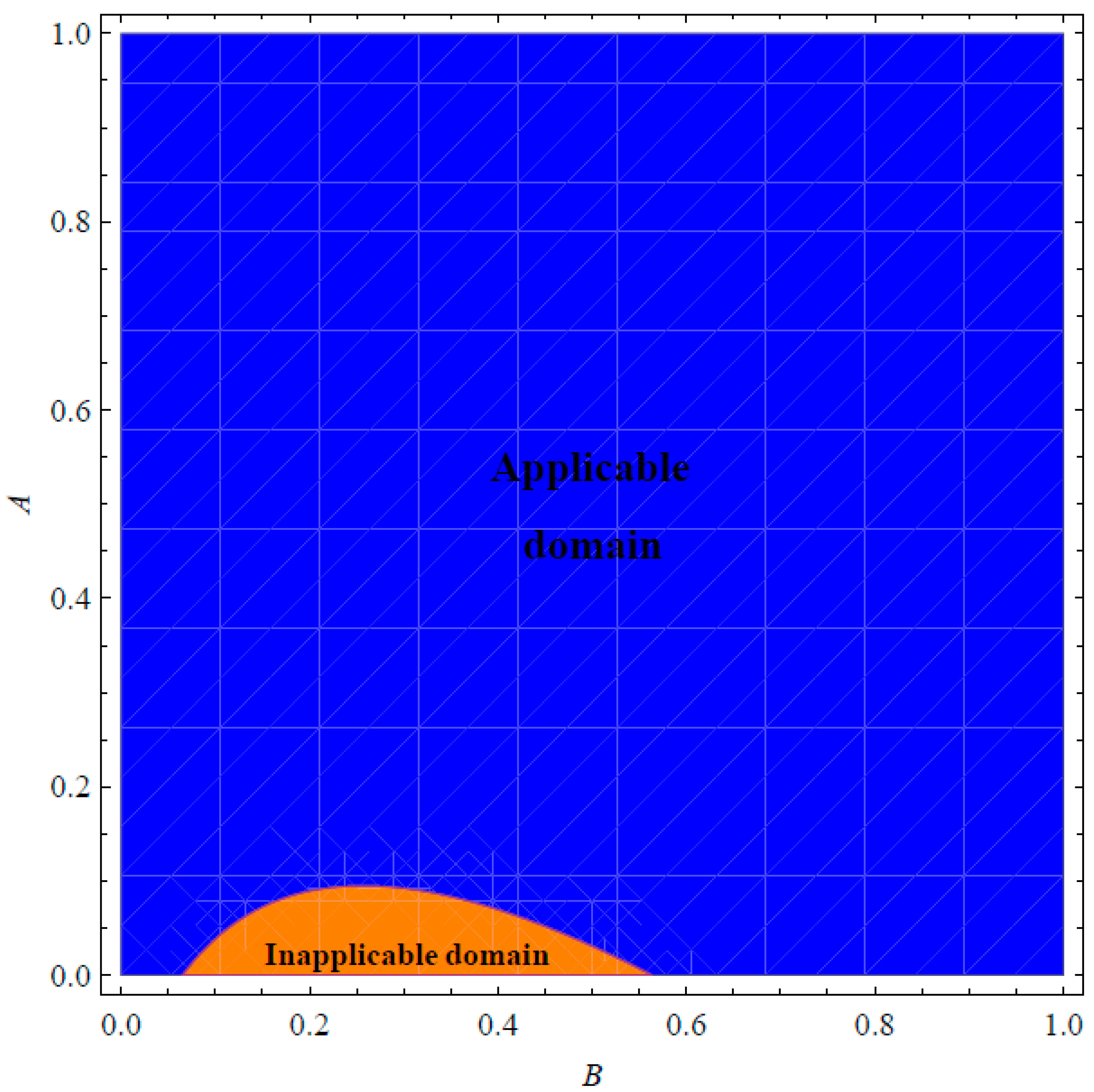
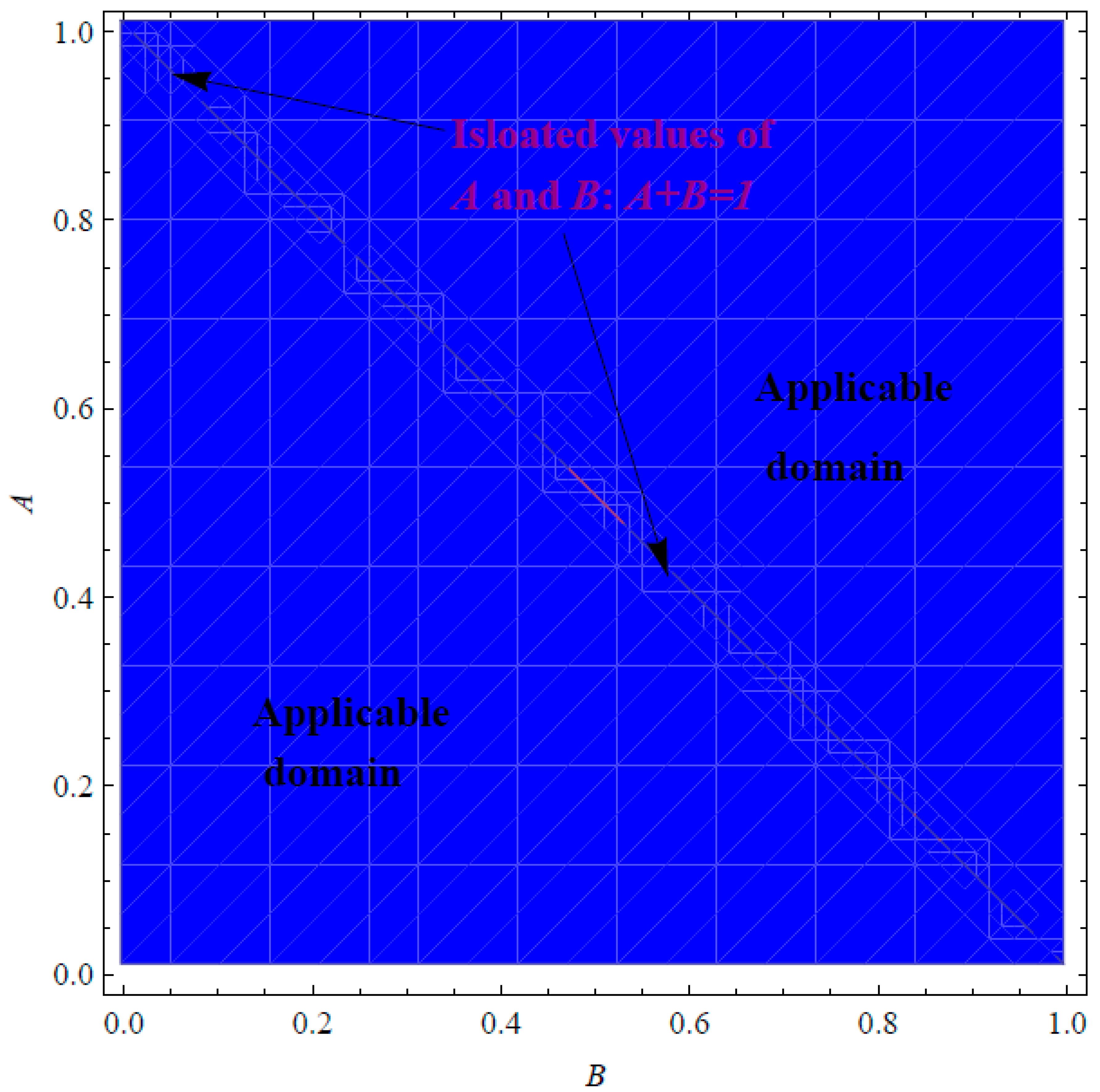
Before launching into the main target of this section, we may shed some light on the domains of applicability/inapplicability for the expressions of and in Equations (31) and (53), respectively. It can be noted from Figure 1 that the approximation is applicable in certain domains for A and B when . However, Figure 2 shows that the corresponding approximation , at , is applicable in all possible domains of A and B provided that is not satisfied, i.e., . Actually, it can be declared that the restriction leads to exact expressions of and . In such cases, the PSS (13) reduces to
while the PSS (15) becomes
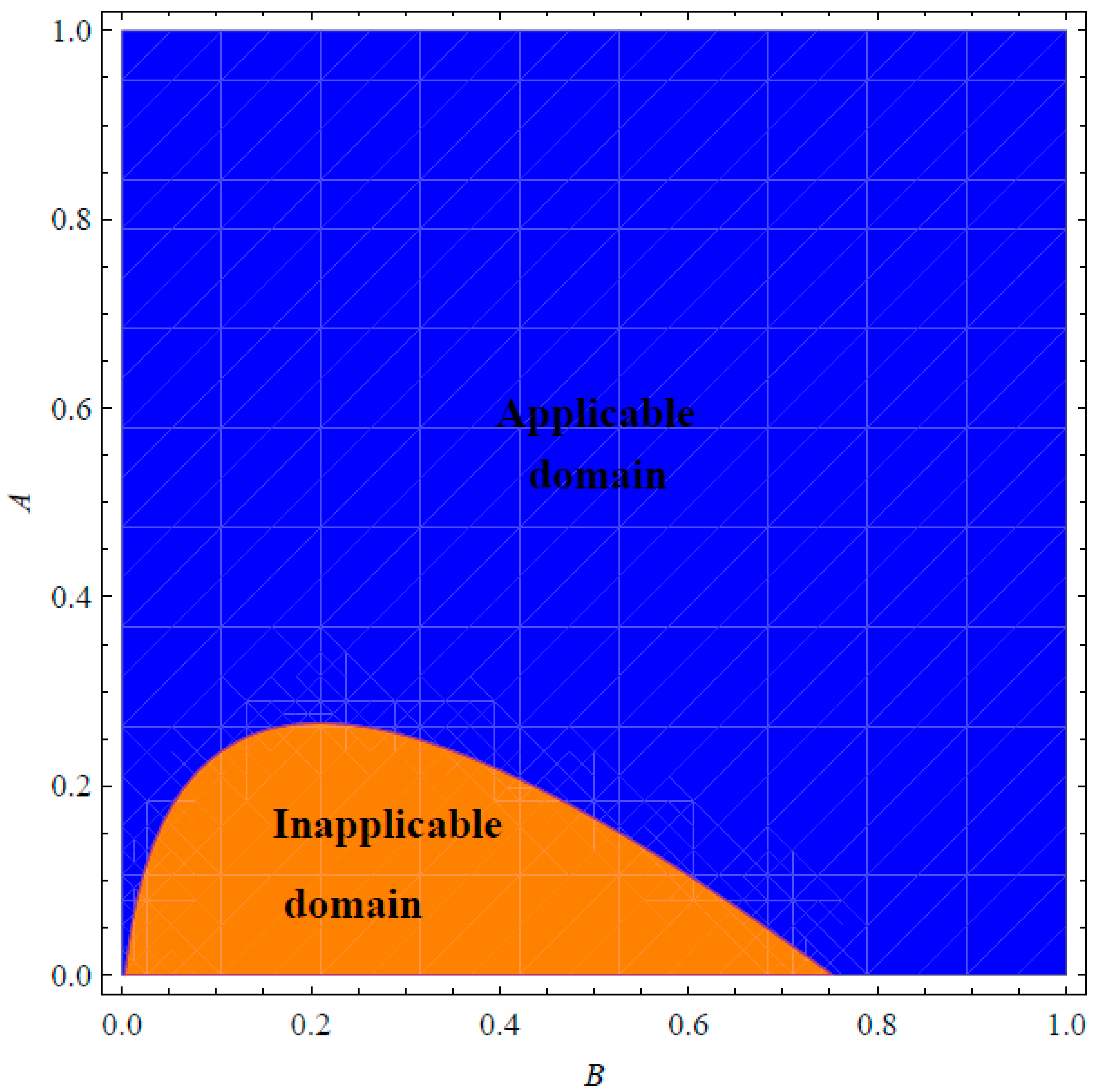
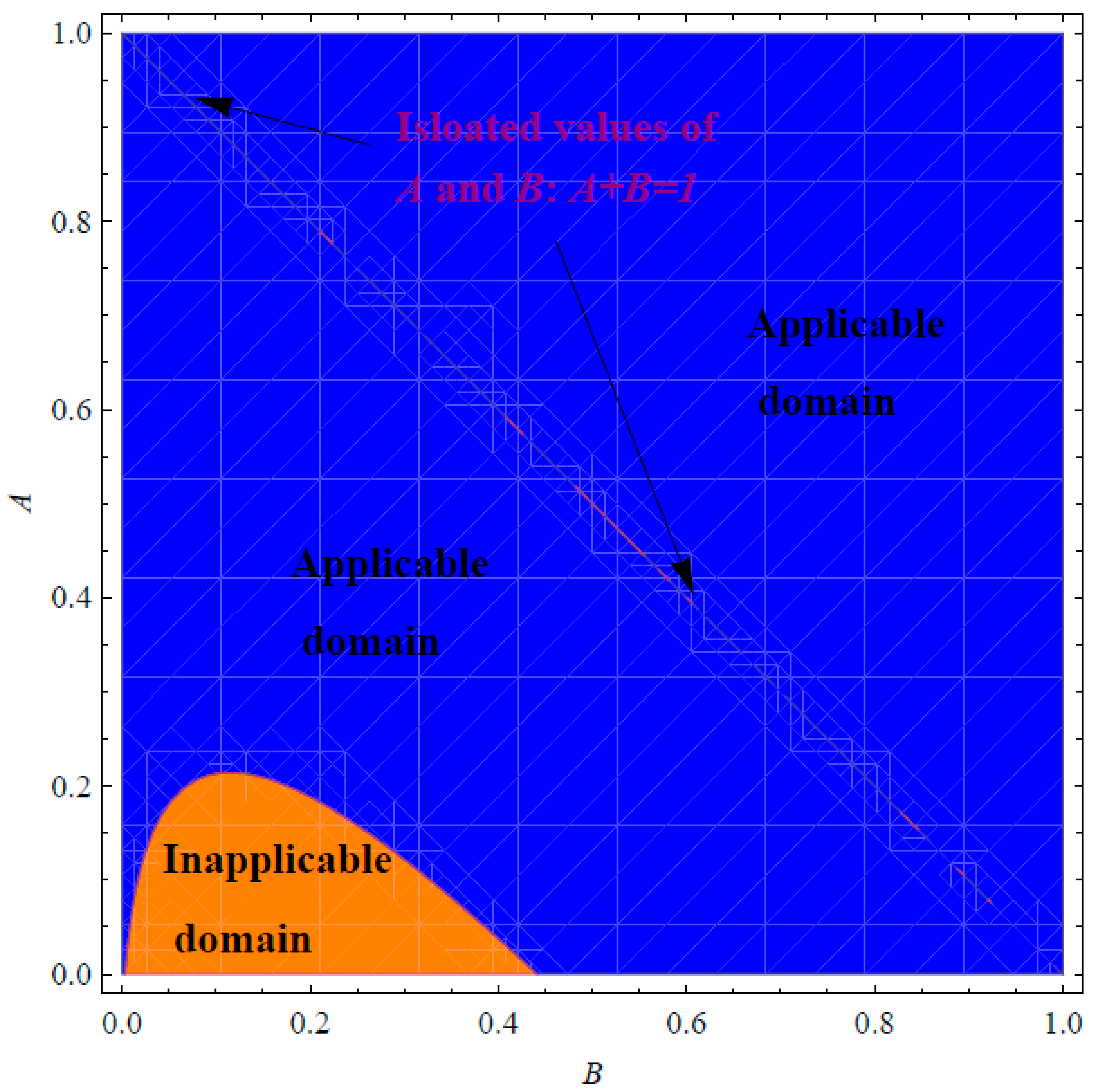
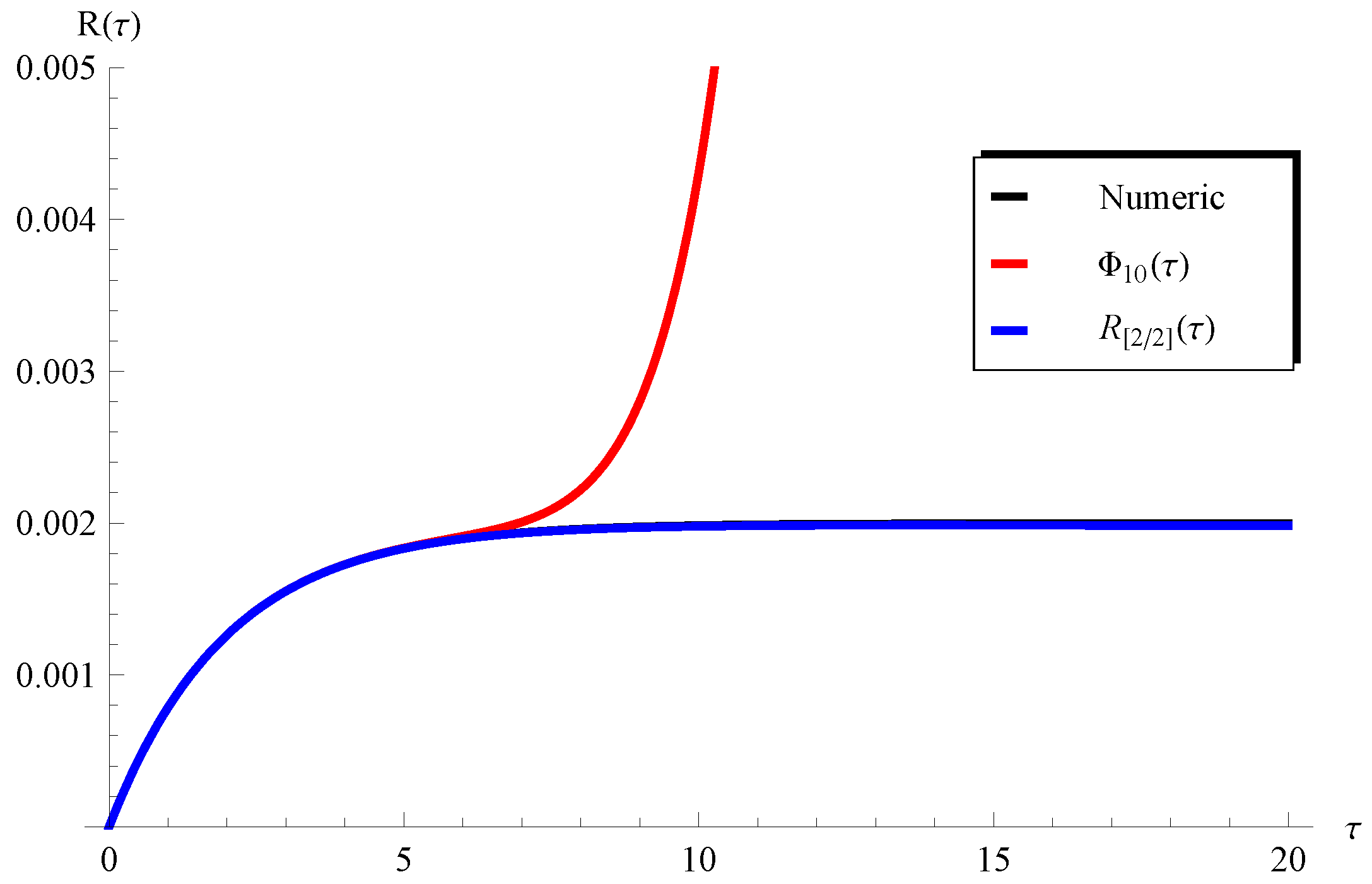
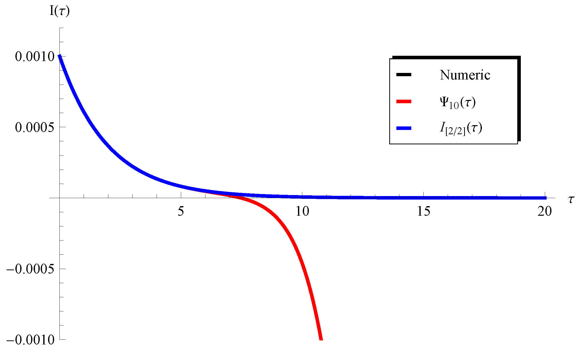
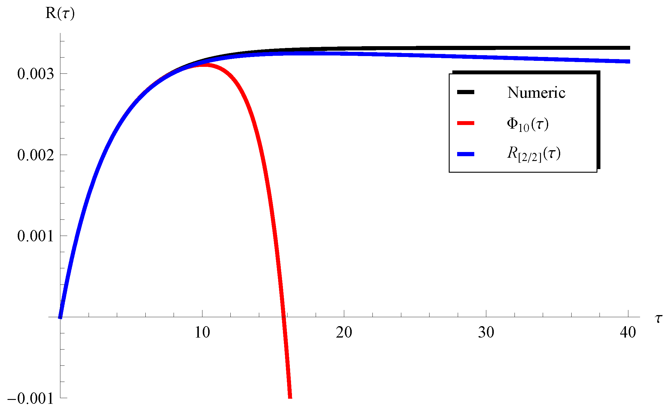
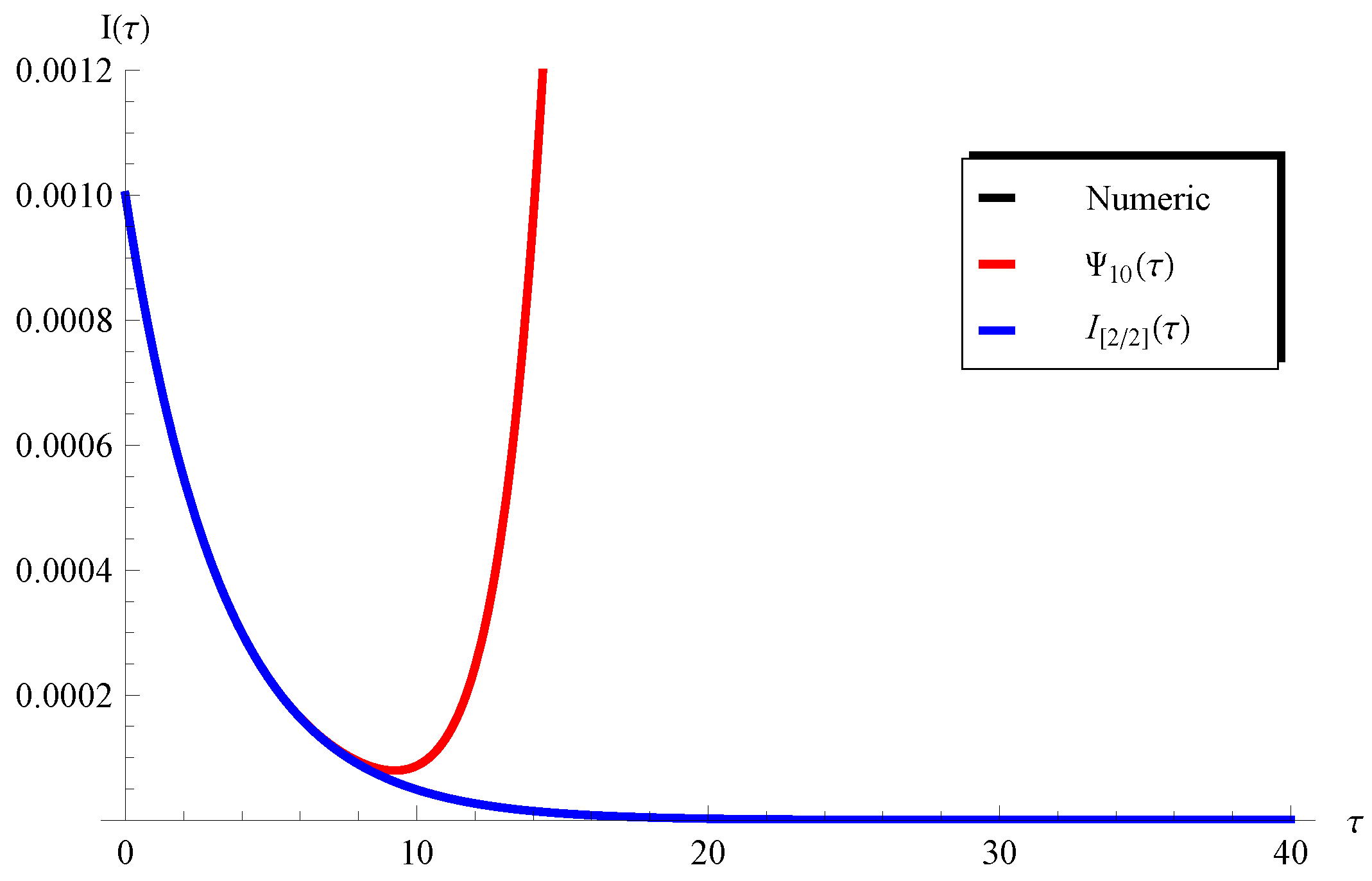
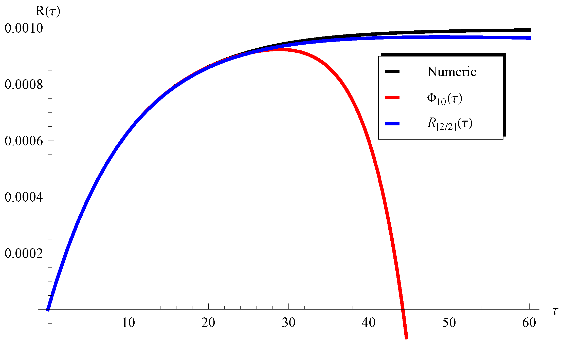
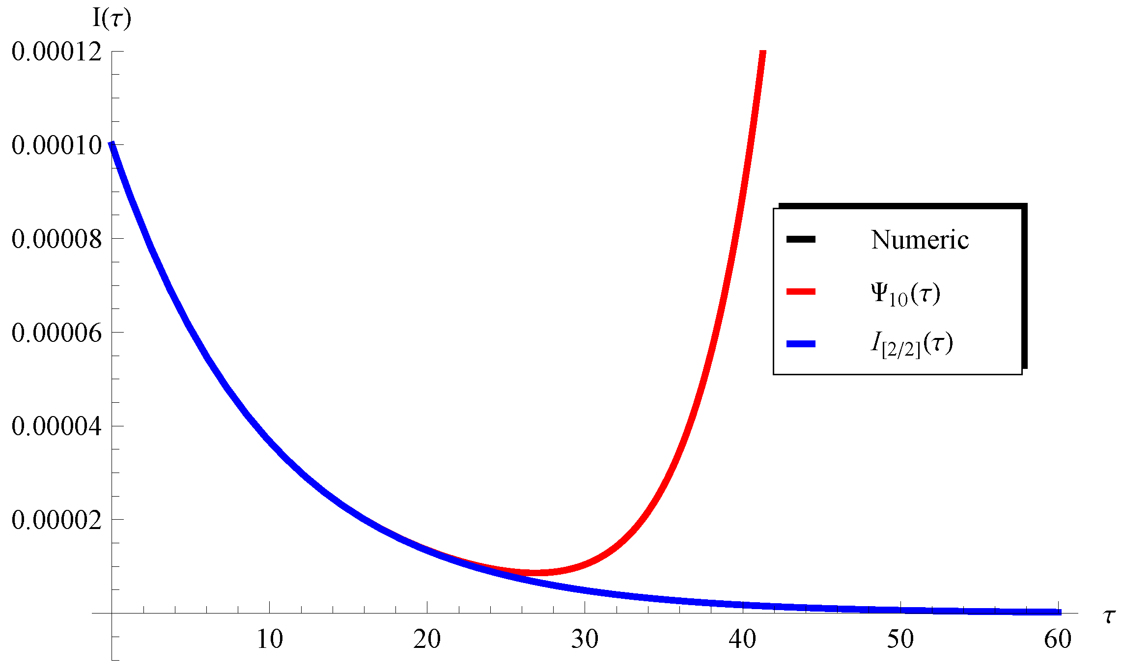
In addition, Figure 3 and Figure 4 show the applicability/inapplicability domains of and at . In Figure 5, the curves of the PSS and the Padé approximant are compared with the numerical solution at , , and . This figure indicates that the domain of agreement with the numerical solution is increased through , while the PSS coincides with the numerical solution in a short domain. Furthermore, Figure 6 confirms this conclusion regarding the Padé approximant and the PSS . Similar results can be seen in Figure 7, Figure 8, Figure 9 and Figure 10. It can be observed from Figure 7 () and Figure 9 () that the difference between the and the numerical solution slightly increases at large values of but the is still better than the PSS .
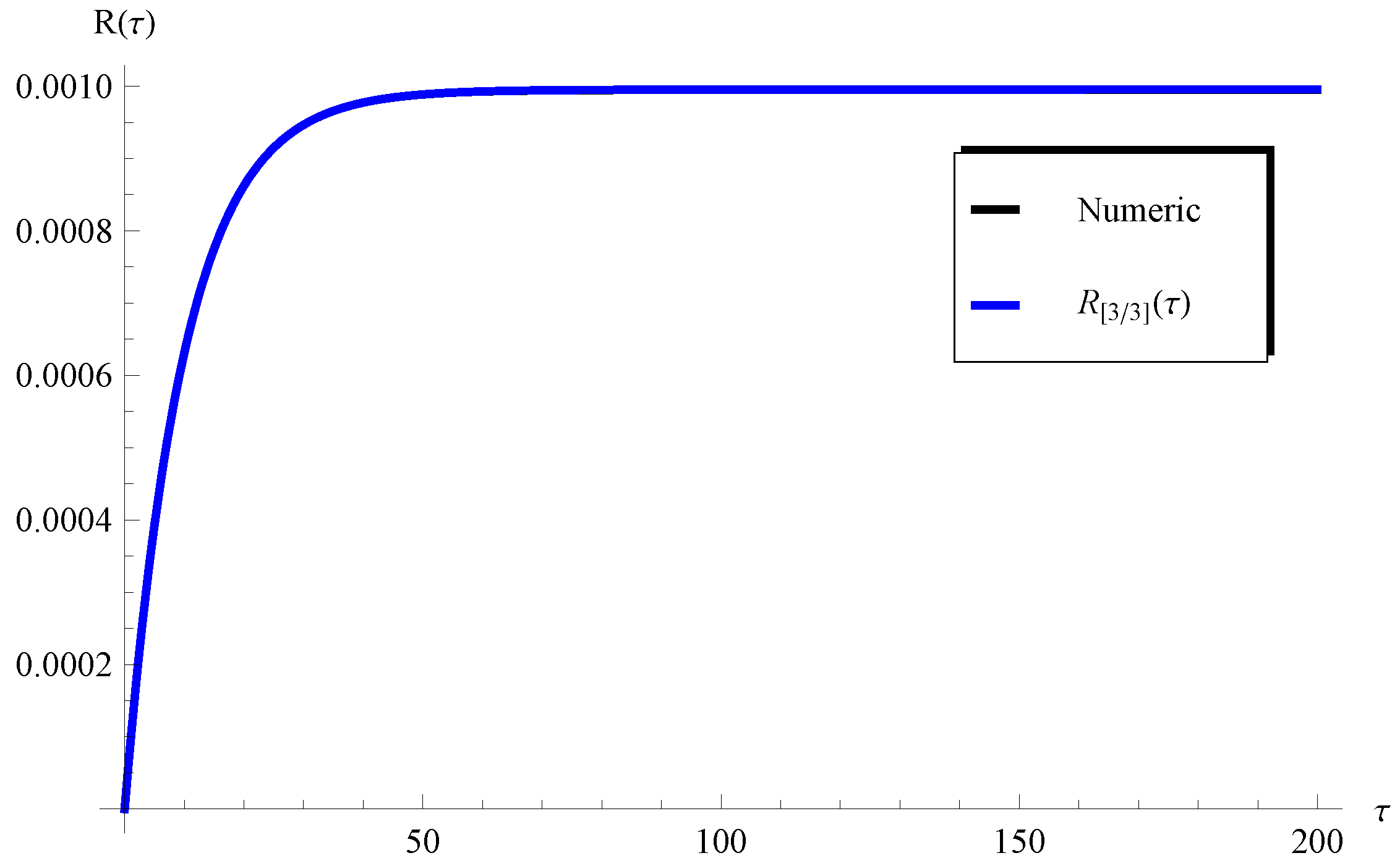
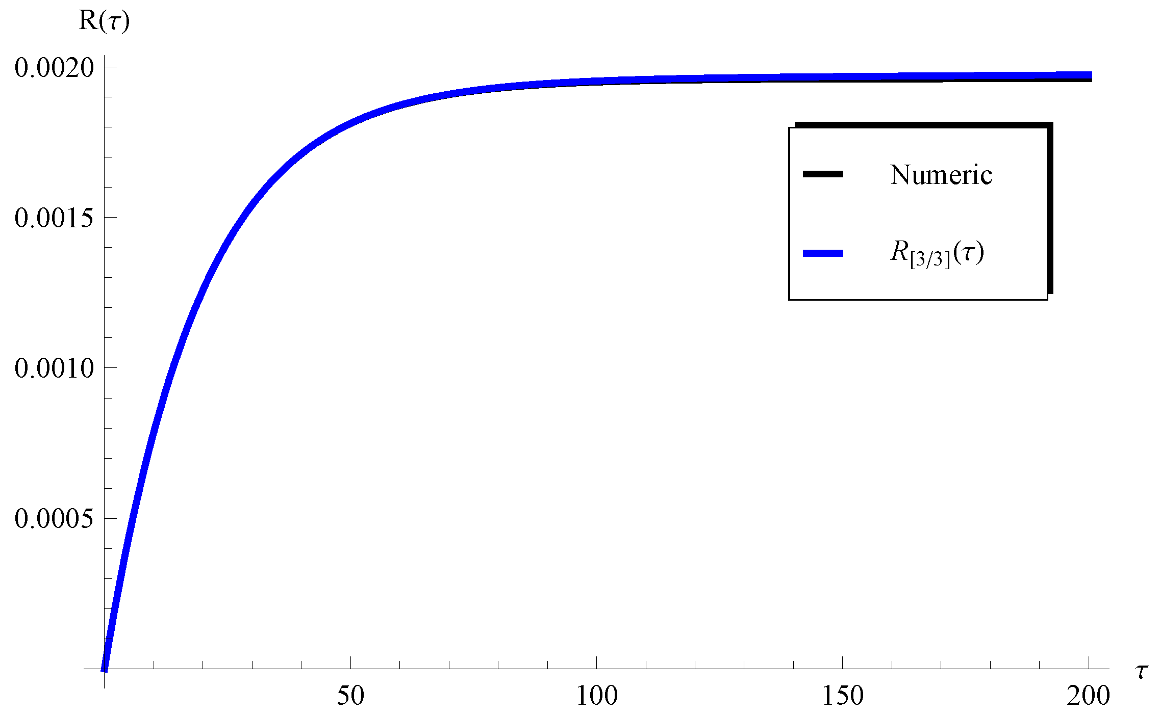
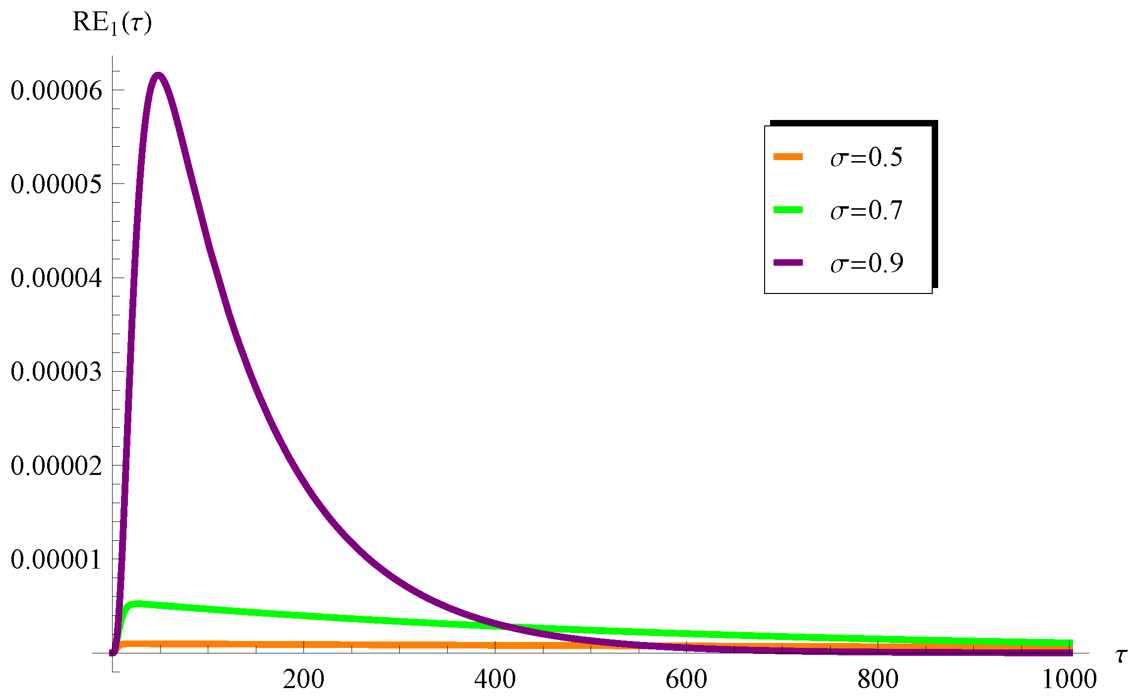
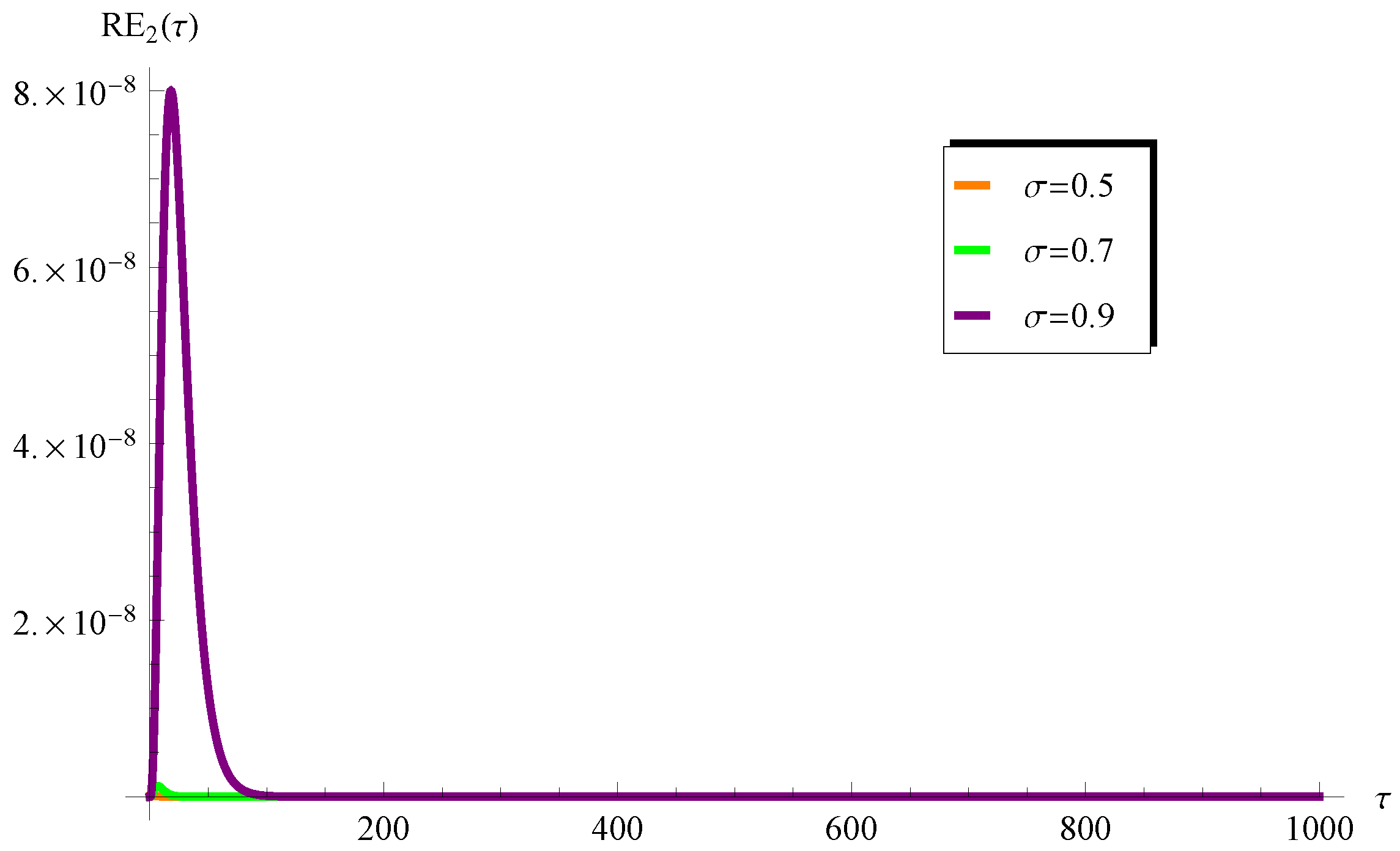
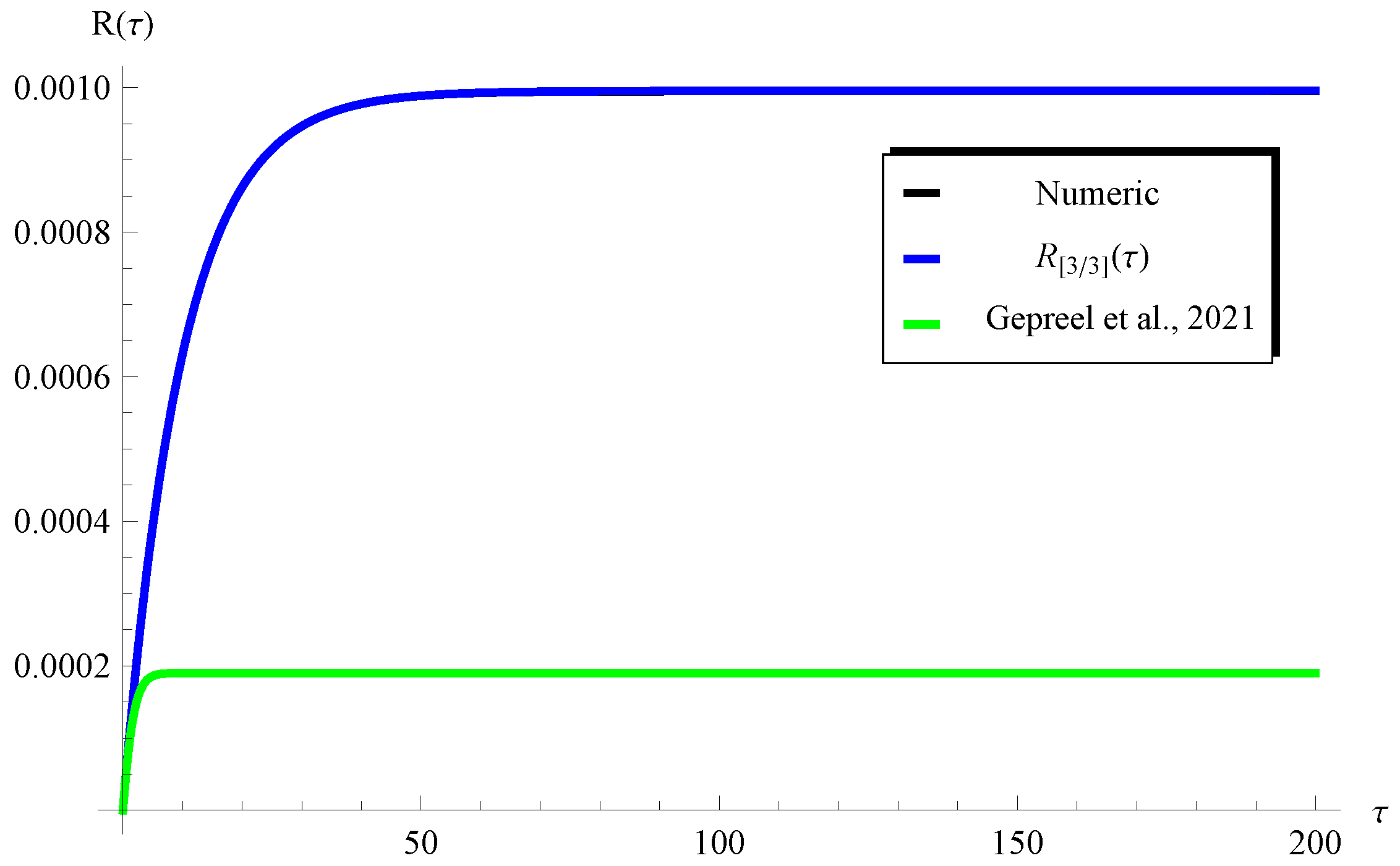
Such a limitation can be easily overcome through considering a higher-order Padé approximant, as will be demonstrated later. On the other hand, one can see from Figure 8 () and Figure 10 () that the curves of the are in full agreement with the numerical ones in the whole domain of . In order overcome the limitations mentioned above, the higher-order Padé approximant is depicted in Figure 11 and Figure 12 at and , respectively. It is clear from these figures that the approximation agrees with the numerical solution in the whole domain. Moreover, the residual error for Equations (1) and (2) is depicted in Figure 13 and Figure 14 using the current Padé approximants and . Furthermore, numerical comparisons are performed between the present PSS , , , and the with the ERKM in Table 1 and Table 2.
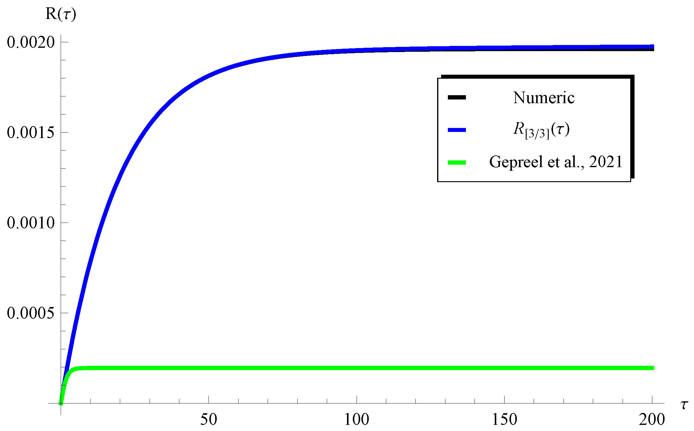
In order to reveal the effectiveness of the our approach over the homotopy perturbation method (HPM) in the literature [23], we present a comparison between the (present), the numerical solution, and the HPM (Ref. [23]) at and in Figure 15 and Figure 16, respectively, when and . These figures show that our solution is closer to the numerical one (nearly identical) when compared with the HPM in Ref. [23].
The above results reveal that the accuracy can be enhanced by applying the current hybrid approach. This is of course one of the main advantages of the proposed method.
5. Conclusions
In this paper, the nonlinear SIR model was solved using a hybrid approach. The proposed technique was based on combining the LT and the Padé approximants. Various analytic approximations were successfully conducted for the infected and the recovered individuals. Moreover, such analytic approximations were found to be applicable in specific domains, which were described analytically and graphically. The performed comparisons with the explicit Runge–Kutta numerical method reveal the accuracy of the obtained results. Furthermore, the calculated residuals confirm this conclusion. The effectiveness of our approach reveals its ability to treat other mathematical and physical models in the applied sciences.
Funding
The author would like to thank Deanship of Scientific Research at Majmaah University for supporting this work under Project Number No. R-2023-483.
Data Availability Statement
Not applicable.
Acknowledgments
The author also would like to thank the referees for their valuable comments and suggestions which helped to improve the manuscript.
Conflicts of Interest
The author declares that there are no competing interest regarding the publication of this paper.
References
- Ebaid, A. Approximate analytical solution of a nonlinear boundary value problem and its application in fluid mechanics. Z. Naturforschung A 2011, 66, 423–426. [Google Scholar] [CrossRef]
- Duan, J.S.; Rach, R. A new modification of the Adomian decomposition method for solving boundary value problems for higher order nonlinear differential equations. Appl. Math. Comput. 2011, 218, 4090–4118. [Google Scholar] [CrossRef]
- Ebaid, A. A new analytical and numerical treatment for singular two-point boundary value problems via the Adomian decomposition method. J. Comput. Appl. Math. 2011, 235, 1914–1924. [Google Scholar] [CrossRef] [Green Version]
- Ali, E.H.; Ebaid, A.; Rach, R. Advances in the Adomian decomposition method for solving two-point nonlinear boundary value problems with Neumann boundary conditions. Comput. Math. Appl. 2012, 63, 1056–1065. [Google Scholar] [CrossRef] [Green Version]
- Chun, C.; Ebaid, A.; Lee, M.; Aly, E.H. An approach for solving singular two point boundary value problems: Analytical and numerical treatment. ANZIAM J. 2012, 53, 21–43. [Google Scholar] [CrossRef] [Green Version]
- Ebaid, A.; Aljoufi, M.D.; Wazwaz, A.-M. An advanced study on the solution of nanofluid flow problems via Adomian’s method. Appl. Math. Lett. 2015, 46, 117–122. [Google Scholar] [CrossRef]
- Bhalekar, S.; Patade, J. An analytical solution of fishers equation using decomposition Method. Am. J. Comput. Appl. Math. 2016, 6, 123–127. [Google Scholar]
- Alshaery, A.; Ebaid, A. Accurate analytical periodic solution of the elliptical Kepler equation using the Adomian decomposition method. Acta Astronaut. 2017, 140, 27–33. [Google Scholar] [CrossRef]
- Bakodah, H.O.; Ebaid, A. Exact solution of Ambartsumian delay differential equation and comparison with Daftardar-Gejji and Jafari approximate method. Mathematics 2018, 6, 331. [Google Scholar] [CrossRef] [Green Version]
- Ebaid, A.; Al-Enazi, A.; Albalawi, B.Z.; Aljoufi, M.D. Accurate approximate solution of Ambartsumian delay differential equation via decomposition method. Math. Comput. Appl. 2019, 24, 7. [Google Scholar] [CrossRef] [Green Version]
- Alenazy, A.H.S.; Ebaid, A.; Algehyne, E.A.; Al-Jeaid, H.K. Advanced Study on the Delay Differential Equation y′(t)=ay(t)+by(ct). Mathematics 2022, 10, 4302. [Google Scholar] [CrossRef]
- Ebaid, A. Remarks on the homotopy perturbation method for the peristaltic flow of Jeffrey fluid with nano-particles in an asymmetric channel. Comput. Math. Appl. 2014, 68, 77–85. [Google Scholar] [CrossRef]
- Nadeem, M.; Li, F. He–Laplace method for nonlinear vibration systems and nonlinear wave equations. J. Low Freq. Noise. Vib. Act. Control. 2019, 38, 1060–1074. [Google Scholar] [CrossRef] [Green Version]
- Ebaid, A.; Aljohani, A.F.; Aly, E.H. Homotopy perturbation method for peristaltic motion of gold-blood nanofluid with heat source. Int. J. Numer. Meth. Heat Fluid Flow 2020, 30, 3121–3138. [Google Scholar] [CrossRef]
- Nadeem, M.; Edalatpanah, S.A.; Mahariq, I.; Aly, W.H.F. Analytical view of nonlinear delay differential equations using Sawi iterative scheme. Symmetry 2022, 14, 2430. [Google Scholar] [CrossRef]
- Liao, S. Beyond Perturbation: Introduction to the Homotopy Analysis Method; CRC Press: Boca Raton, FL, USA, 2003. [Google Scholar]
- Chauhan, A.; Arora, R. Application of homotopy analysis method (HAM) to the non-linear KdV equations Astha Chauhan and Rajan Arora. Commun. Math. 2023, 31, 205–220. [Google Scholar] [CrossRef]
- Ebaid, A. Approximate periodic solutions for the non-linear relativistic harmonic oscillator via differential transformation method. Commun. Nonlinear Sci. Numer. Simul. 2010, 15, 1921–1927. [Google Scholar] [CrossRef]
- Ebaid, A. A reliable aftertreatment for improving the differential transformation method and its application to nonlinear oscillators with fractional nonlinearities. Commun. Nonlinear Sci. Numer. Simul. 2011, 16, 528–536. [Google Scholar] [CrossRef]
- Liu, Y.; Sun, K. Solving power system differential algebraic equations using differential transformation. IEEE Trans. Power Syst. 2020, 35, 2289–2299. [Google Scholar] [CrossRef]
- Benhammouda, B. The differential transform method as an effective tool to solve implicit Hessenberg index-3 differential-algebraic equations. J. Math. 2023, 2023, 3620870. [Google Scholar] [CrossRef]
- Abajo, J.G.D. Simple mathematics on COVID-19 expansion. MedRxiv 2020. [Google Scholar] [CrossRef]
- Gepreel, K.A.; Mohamed, M.S.; Alotaibi, H.; Mahdy, A.M.S. Dynamical behaviors of nonlinear coronavirus (COVID-19) model with numerical studies. Comput. Mater. Contin. 2021, 67, 675–686. [Google Scholar] [CrossRef]
Figure 1.
Applicability/inapplicability domains of the at .

Figure 2.
Applicability/inapplicability domains of the at .

Figure 3.
Applicability/inapplicability domains of the at .

Figure 4.
Applicability/inapplicability domains of the at .

Figure 5.
Plots of the PSS , the , and the numerical solution at , , and .

Figure 6.
Plots of the PSS , the , and the numerical solution at , , and .

Figure 7.
Plots of the PSS , the , and the numerical solution at , , and .

Figure 8.
Plots of the PSS , the , and the numerical solution at , , and .

Figure 9.
Plots of the PSS , the , and the numerical solution at , , and .

Figure 10.
Plots of the PSS , the , and the numerical solution at , , and .

Figure 11.
Plots of the and the numerical solution at , , and .

Figure 12.
Plots of the and the numerical solution at , , and .

Figure 13.
Variation in the residual at various values of when and .

Figure 14.
Variation of the residual at various values of when and .

Figure 15.
Comparison between the (present), the numerical solution, and the HPM (Ref. [23]) at , , and .
Figure 15.
Comparison between the (present), the numerical solution, and the HPM (Ref. [23]) at , , and .

Figure 16.
Comparison between the (present), the numerical solution, and the HPM (Ref. [23]) at , , and .
Figure 16.
Comparison between the (present), the numerical solution, and the HPM (Ref. [23]) at , , and .


Table 1.
Comparisons of the present PSS and the LT-Padé approximant with the ERKM at , and .
| (Present) | (Present) | ERKM (Numerical) | |
|---|---|---|---|
| 5 | 0.0018364 | 0.0018327 | 0.0018338 |
| 10 | 0.0043093 | 0.0019785 | 0.0019837 |
| 15 | 0.1220652 | 0.0019860 | 0.0019959 |
| 20 | 1.9188949 | 0.0019820 | 0.0019969 |
| 25 | 16.160833 | 0.0019772 | 0.0019970 |
| 30 | 91.203779 | 0.0019722 | 0.0019970 |
| 35 | 390.97111 | 0.0019673 | 0.0019970 |
| 40 | 1372.0035 | 0.0019624 | 0.0019970 |
| 45 | 4135.3979 | 0.0019575 | 0.0019970 |
| 50 | 11061.598 | 0.0019526 | 0.0019970 |
Table 2.
Comparisons of the present PSS and the LT-Padé approximant with the ERKM at , and .
| (Present) | (Present) | ERKM (Numerical) | |
|---|---|---|---|
| 5 | |||
| 10 | |||
| 15 | |||
| 20 | |||
| 25 | |||
| 30 | |||
| 35 | |||
| 40 | |||
| 45 | |||
| 50 |
Disclaimer/Publisher’s Note: The statements, opinions and data contained in all publications are solely those of the individual author(s) and contributor(s) and not of MDPI and/or the editor(s). MDPI and/or the editor(s) disclaim responsibility for any injury to people or property resulting from any ideas, methods, instructions or products referred to in the content. |
© 2023 by the author. Licensee MDPI, Basel, Switzerland. This article is an open access article distributed under the terms and conditions of the Creative Commons Attribution (CC BY) license (https://creativecommons.org/licenses/by/4.0/).
Share and Cite
MDPI and ACS Style
Albidah, A.B. A Proposed Analytical and Numerical Treatment for the Nonlinear SIR Model via a Hybrid Approach. Mathematics 2023, 11, 2749. https://doi.org/10.3390/math11122749
AMA Style
Albidah AB. A Proposed Analytical and Numerical Treatment for the Nonlinear SIR Model via a Hybrid Approach. Mathematics. 2023; 11(12):2749. https://doi.org/10.3390/math11122749
Chicago/Turabian StyleAlbidah, Abdulrahman B. 2023. "A Proposed Analytical and Numerical Treatment for the Nonlinear SIR Model via a Hybrid Approach" Mathematics 11, no. 12: 2749. https://doi.org/10.3390/math11122749
Note that from the first issue of 2016, this journal uses article numbers instead of page numbers. See further details here.