Construction of Local-Shape-Controlled Quartic Generalized Said-Ball Model

Abstract

Said-Ball curves and surfaces are extensively applied in the realm of geometric modeling. Their appearance is only decided by the control points, which produces a great deal of inconvenience for the shape design of sophisticated products. To overcome this defect, we construct a novel kind of quartic generalized Said-Ball (QGS-Ball, for short) curves and surfaces, which contain multiple shape parameters, and the global and local shape can be easily modified via shape parameters. The specific research contents are as follows: Firstly, the QGS-Ball basis functions carrying multiple shape parameters are defined, and the correlative properties are proved. Secondly, the QGS-Ball curve is proposed according to the QGS-Ball basis functions, and the effect of shape parameters on the curve is discussed. Thirdly, in view of the constructed QGS-Ball curve, we further propose the combined quartic generalized Said-Ball (CQGS-Ball, for short) curves, and deduce the conditions of first-order and second-order geometric continuity (namely, G¹ and G² continuity). Finally, the QGS-Ball surface is defined by tensor product method, and the influence of shape parameters on the surface is analyzed. The main contribution of this article is to construct the QGS-Ball curve model, and deduce the G¹ and G² geometric joining conditions of QGS-Ball curves. Combined with some modeling examples, it further illustrates that the QGS-Ball curve as a new geometric model provides a powerful supplement for the geometric design of sophisticated form in computer-aided design (CAD) and computer-aided manufacturing (CAM) systems.

1. Introduction

Computer-aided geometric design (CAGD) was first raised by Riesenfeld and Barnhill at an international conference in 1974, and had a significant impact on the traditional manufacturing industry once it came out, furthering the development of product appearance design technology [1]. Free-form curves and surfaces are the focus of CAGD, which have mainly experienced several important development stages, such as Ferguson, Coons, Bézier, B-spline, and NURBS curves and surfaces. Among them, Bézier curves have many advantages, such as simple structure, intuitive graphics, and excellent geometric properties, and have been widely used in CAGD. Similar to Bézier curves and surfaces, Ball curves and surfaces have also received extensive attention and application in the shape design of industrial products.

In 1974, the mathematician Ball constructed the rational cubic Ball curve [2,3,4]. Since the traditional Ball curve is cubic, it cannot meet the construction requirements of complex curves in industrial design and other realms. Therefore, Wang proposed a higher-order Ball curve by expanding the order of the traditional Ball basis functions, called the Wang-Ball curve [5]. Said constructed the Ball basis functions with arbitrary odd order, and obtained the Said-Ball curve, which has many excellent properties [6]. Hu further perfected and proposed the Said-Ball curve with arbitrary order in 1996 [7]. Later, the Said-Ball curve and its application were discussed in [8]. In order to further promote the application of Said-Ball curves, Hu derived the mathematical expressions of the rational cubic and quartic Said-Ball conic curves, which combined the rational low-order Bézier conic curves and the conversion formula of the two types of basis functions [9]. On the basis of the characteristics of Wang-Ball curves and Said-Ball curves, Wu proposed the Said-Bézier/Wang-Said generalized Ball curves [10]. However, the order of generalized Ball curves and surfaces can be increased or decreased, and their flexibility and shape adjustability are very limited. When the relevant Ball basis functions are given, if the geometric appearance of curves and surfaces need to be modified, we can only adjust their control points. Hence, researchers proposed the generalized Ball curves and surfaces carrying the shape parameters.

The main feature of generalized Ball curves and surfaces with parameters is that its shape can be slickly modified via shape parameters. At present, domestic and foreign scholars have carried out abundant explorative work on the generalized Ball curves and surfaces to meet the requirements of practical applications. In 2004, Wu defined the dual basis of a class of generalized Ball curves, which contains a parameter k, and the corresponding Markov identities, the transformation expressions of the bases, and control points of different curves were also attained in view of the dual basis [11]. Wang proposed the quartic Ball basis functions carrying a parameter $\lambda$, as well as constructed the quartic Ball curve in view of the basis functions, and the curve can be modified via $\lambda$ [12]. Two types of curves were constructed in 2009; the first is the ninth-order Wang-Ball and Said-Ball curves and a great deal of curves between them; the second is the ninth-order Said-Ball and Bézier curves and a great deal of curves between them. They all only have one shape parameter [13]. In view of the envelope and topological mapping theory, the characteristics of the quartic Ball curve and the influence of shape parameter $\lambda$ were studied, and the final conclusion shows that the shape adjustability of the quartic Ball curve is outstanding [14]. In addition, Xiong and Guo [15] proposed the n-degree Said-Ball curve containing a parameter, which further expanded the Said-Ball curves. Meanwhile, Xiong and Guo proposed the n-degree Wang-Ball curves with a parameter [16]. Cao studied the variational problem of Ball surface with the minimum energy under control constraints, the hybrid Ball surface was firstly proposed, and then the Ball surface with minimum energy was obtained by modifying the unfixed control ball, where w is the shape parameter [17].

Generalized Ball curves and surfaces carrying a parameter have the merit of improving the shape adjustability, but the defect is that the shape modifiability is very limited, which cannot meet the needs of people. In 2011, Liu proposed the quartic Q-Ball curve, which contains two control parameters $\lambda$ and $\mu$, so the shape adjustability of the curve is improved [18]. The quartic Wang-Ball curve and surface with $\alpha$, $\beta$ were proposed, and the main characteristic different from the quartic Ball curve and surface is that the curve and surface can be flexibly adjusted via the parameters $\alpha$ and $\beta$ [19]. In 2016, Wang and Chen constructed the shape-adjustable quintic Said-Ball curves and surfaces containing two parameters, as well as the G¹ (i.e., two adjacent curves have the same unit tangent at the common connection point) and G² (i.e., two adjacent curves have a common curvature vector at the connection point under the condition of G¹ continuity); the joining conditions of two neighboring quintic Said-Ball curves were further given in [20]. The quartic generalized Ball surface carrying two parameters has the outstanding features of the Ball surface, and has the fine property of flexibly controlling the Ball surface shape [21]. Hu and Du constructed a Said-Ball curve with two parameters, discussed its geometric properties, and studied the relevant algorithms [22]. At this time, although the adaptability and shape adjustability of the generalized Ball curves and surfaces carrying two parameters have been widely elevated, the shape adjustability is still restricted, which undoubtedly limits its application in geometric modeling. Therefore, the generalized cubic Ball basis functions and the corresponding generalized cubic developable Ball surface containing multiple shape parameters were proposed, and a boosting marine predator algorithm can optimize the developable surface [23]. Unlike the traditional Said-Ball curve, the proposed 2m + 2-order Said-Ball curve carrying multiple shape parameters can modify the curve by the parameters [24]. Later, Hu et al. constructed the cubic generalized Ball curves via introducing multiple parameters, and the curves can also be optimized by a hybrid manta ray foraging optimization algorithm [25].

In this work, we reconstruct the QGS-Ball basis functions containing three shape parameters, and propose the shape-modifying QGS-Ball curve and surface, whose global and local shape can be modified by three shape parameters. In addition, we further define the CQGS-Ball curves, then the G¹ and G² geometric joining problem of QGS-Ball curves is discussed. The main highlights of this work are below:

• The QGS-Ball basis functions are proposed by introducing three shape parameters.
• The QGS-Ball curves and surfaces are proposed, and the impact of shape parameters on the curves and surfaces is discussed.
• The CQGS-Ball curves are defined based on the novel QGS-Ball curves, and the continuity conditions of G¹ and G² smooth joining of QGS-Bal curves are derived.

The rest of the paper is organized as follows: Section 2 presents the expression and properties of the QGS-Ball basis functions, and the related properties are proved in detail. Section 3 displays the definition and properties of QGS-Ball curves, and analyzes the impact of shape parameters on the curve combining theory and examples. The CQGS-Ball curves are defined, and the G¹ and G² geometric joining conditions of QGS-Ball curves are derived in Section 4. Section 5 presents the definition and properties of QGS-Ball surfaces, and discusses the impact of shape parameters on the surface. The conclusions and future work are discussed in Section 6.

2. Quartic Generalized Said-Ball Basis Functions

By introducing multiple shape parameters, we construct the quartic generalized Said-Ball basis functions, and describe the definition and properties in detail.

2.1. Definition of QGS-Ball Basis Functions

Definition 1. 

For $\tau \in [0, 1]$, the quartic generalized Said-Ball (QGS-Ball, for short) basis functions are given by the following equation:

$$\begin{array}{l}{f}_{0,4}(\tau )=(1-{\lambda }_1\tau ){(1-\tau )}^3,\\ f_{1,4}(\tau )=\left[3-({\lambda }_2+3)\tau +{\lambda }_1(1-\tau )\right]\tau {(1-\tau )}^2,\\ f_{2,4}(\tau )=(6+2{\lambda }_2){\tau }^2{(1-\tau )}^2,\\ f_{3,4}(\tau )=\left[(3+{\lambda }_3)\tau -{\lambda }_2(1-\tau )\right]{\tau }^2(1-\tau ),\\ f_{4,4}(\tau )=(1-{\lambda }_3+{\lambda }_3\tau ){\tau }^3.\end{array}$$

(1)

where, ${\lambda }_1, {\lambda }_2 \mathit{and} {\lambda }_3$ are the shape parameters, ${\lambda }_1,{\lambda }_3\in [-3, 1],{\lambda }_2\in [-3, 0]$.

Figure 1 displays the QGS-Ball basis functions corresponding to different shape parameter values. For convenience, the shape parameters in Figure 1 are marked as $\Theta =\{{\lambda }_1,{\lambda }_2,{\lambda }_3\}$.

2.2. Properties of QGS-Ball Basis Functions

Theorem 1. 

The QGS-Ball basis functions possess the following properties:

(1) 

Non-negativity: For $\tau \in [0, 1]$, there are $f_{i,4}(\tau )\ge 0, i=0, 1, 2, 3, 4$, where ${\lambda }_1, {\lambda }_3\in [-3, 1],$${\lambda }_2\in [-3, 0]$.

(2) 

Normality: ${\displaystyle \sum _{i=0}^4{f}_{i,4}(\tau )}\equiv 1$.

(3) 

Symmetry under the particular case: When ${\lambda }_1={\lambda }_3, {\lambda }_2=0$, the QGS-Ball basis functions $f_{i,4}(\tau )$$i=0, 1, 2, 3, 4$ are symmetric, that is, $f_{0,4}(\tau )=f_{4,4}(1-\tau )$ and $f_{1,4}(\tau )=f_{3,4}(1-\tau )$.

(4) 

Endpoint properties:

$$\begin{array}{lll}{f}_{i,4}(0)=\left\{\begin{array}{lll}1,& & if i=0,\\ 0,& & else,\end{array}\right.& & f_{i,4}(1)=\left\{\begin{array}{lll}1,& & ifi=4,\\ 0,& & else,\end{array}\right.\\ f_{i,4}^{\prime }(0)=\left\{\begin{array}{lll}-{\lambda }_1-3,& & if i=0,\\ {\lambda }_1+3,& & if i=1,\\ 0,& & if i=2, 3, 4,\end{array}\right.& & f_{i,4}^{\prime }(1)=\left\{\begin{array}{lll}-{\lambda }_3-3,& & if i=3,\\ {\lambda }_3+3,& & if i=4,\\ 0,& & if i=0, 1, 2,\end{array}\right.\\ f_{i,4}^{″}(0)=\left\{\begin{array}{lll}6{\lambda }_1+6,& & if i=0,\\ -6{\lambda }_1-2{\lambda }_2-18,& & if i=1,\\ 4{\lambda }_2+12,& & if i=2,\\ -2{\lambda }_2,& & if i=3,\\ 0,& & if i=4,\end{array}\right.& & f_{i,4}^{″}(1)=\left\{\begin{array}{lll}0,& & if i=0,\\ -2{\lambda }_2,& & if i=1,\\ 4{\lambda }_2+12,& & if i=2,\\ -6{\lambda }_3-2{\lambda }_2-18,& & if i=3,\\ 6{\lambda }_3+6,& & if i=4.\end{array}\right.\end{array}$$

(2)

(5) 

Unimodal property: The QGS-Ball basis functions $f_{i,4}(\tau ), i=0, 1, 2, 3, 4$ have only one maximum value on $[0, 1]$.

(6) 

Monotonicity of parameters: Consider $\tau$ as a constant, $f_{0,4}(\tau )$ is a decreasing function about ${\lambda }_1$, $f_{1,4}(\tau )$ is an increasing function about ${\lambda }_1$ and a decreasing function about ${\lambda }_2$, $f_{2,4}(\tau )$ is an increasing function about ${\lambda }_2$, $f_{3,4}(\tau )$ is a decreasing function about ${\lambda }_2$ and an increasing function about ${\lambda }_3$, and $f_{4,4}(\tau )$ is a decreasing function about ${\lambda }_3$.

(7) 

Degeneracy: The QGS-Ball basis functions reduce into the traditional quartic Said-Ball basis functions when ${\lambda }_1={\lambda }_2={\lambda }_3=0$. It reduces into the quartic Bernstein basis functions when ${\lambda }_1={\lambda }_3=1, {\lambda }_2=0$. It reduces into the cubic Bernstein basis functions when ${\lambda }_1={\lambda }_3=0,$ ${\lambda }_2=-3$.

Proof of Theorem 1. 

(1)

Because of $0\le \tau \le 1$, ${\lambda }_1, {\lambda }_3\in [-3, 1]$ and ${\lambda }_2\in [-3, 0]$, there are

$0\le 1-\tau \le 1$, $0\le {(1-\tau )}^3\le 1$, $1-{\lambda }_1\tau \ge 0$, that is, $f_{0,4}(\tau )\ge 0$.

$3-({\lambda }_2+3)\tau +{\lambda }_1(1-\tau )=(3+{\lambda }_1)(1-\tau )-{\lambda }_2\tau \ge 0$, $\tau {(1-\tau )}^2\ge 0$, that is, $f_{1,4}(\tau )\ge 0$.

$6+2{\lambda }_2\ge 0,$ $(6+2{\lambda }_2){\tau }^2{(1-\tau )}^2\ge 0$, that is, $f_{2,4}(\tau )\ge 0$.

$(3+{\lambda }_3)\tau \ge 0,{\lambda }_2(1-\tau )\le 0,$ $(3+{\lambda }_3)\tau -{\lambda }_2(1-\tau )\ge 0$, ${\tau }^2(1-\tau )\ge 0$, that is, $f_{3,4}(\tau )\ge 0$.

$1-{\lambda }_3+{\lambda }_3\tau \ge 0$, that is, $f_{4,4}(\tau )\ge 0$.

Therefore, $f_{i,4}(\tau )\ge 0,i=0,1, 2, 3, 4$.

(2)

According to Equation (1), there are

$$\begin{array}{l}{f}_{0,4}(\tau )=1-({\lambda }_1+3)\tau +(3{\lambda }_1+3){\tau }^2-(3{\lambda }_1+1){\tau }^3+{\lambda }_1{\tau }^4,\\ f_{1,4}(\tau )=({\lambda }_1+3)\tau -(9+3{\lambda }_1+{\lambda }_2){\tau }^2+(9+3{\lambda }_1+2{\lambda }_2){\tau }^3-({\lambda }_1+{\lambda }_2+3){\tau }^4,\\ f_{2,4}(\tau )=(6+2{\lambda }_2){\tau }^2-(4{\lambda }_2+12){\tau }^3+(6+2{\lambda }_2){\tau }^4,\\ f_{3,4}(\tau )=-{\lambda }_2{\tau }^2+(2{\lambda }_2+3+{\lambda }_3){\tau }^3-(3+{\lambda }_2+{\lambda }_3){\tau }^4,\\ f_{4,4}(\tau )=(1-{\lambda }_3){\tau }^3+{\lambda }_3{\tau }^4,\end{array}$$

(3)

By summing all the basis functions in Equation (3), we can obtain ${\displaystyle \sum _{i=0}^4{f}_{i,4}(\tau )}\equiv 1$.

(3)

When ${\lambda }_1={\lambda }_3, {\lambda }_2=0$, Equation (1) can be written as

$$\begin{array}{l}{f}_{0,4}(\tau )=(1-{\lambda }_1\tau ){(1-\tau )}^3,\\ f_{1,4}(\tau )=\left[3-3\tau +{\lambda }_1(1-\tau )\right]\tau {(1-\tau )}^2,\\ f_{2,4}(\tau )=6{\tau }^2{(1-\tau )}^2,\\ f_{3,4}(\tau )=(3+{\lambda }_1){\tau }^3(1-\tau ),\\ f_{4,4}(\tau )=(1-{\lambda }_1+{\lambda }_1\tau ){\tau }^3.\end{array}$$

(4)

It can be seen from Equation (4) that $f_{0,4}(\tau )=f_{4,4}(1-\tau ), f_{1,4}(\tau )=f_{3,4}(1-\tau )$, so the symmetry is verified in the particular case.

(4)

The endpoint properties can be obtained by simple calculation of $f_{i,4}(\tau ), i=0, 1, 2, 3, 4$.

(5)

The unimodality of QGS-Ball basis functions can be verified by derivation. $f_{3,4}(\tau )$ and $f_{4,4}(\tau )$ have unimodality according to the property (3), so it is only necessary to prove that $f_{0,4}(\tau ), f_{1,4}(\tau )$ and $f_{2,4}(\tau )$ have unimodality.

(6)

If $\tau$ is regarded as a constant, $f_{0,4}(\tau )$ is a decreasing function about ${\lambda }_1$, $f_{1,4}(\tau )$ is an increasing function about ${\lambda }_1$ and a decreasing function about ${\lambda }_2$, $f_{2,4}(\tau )$ is an increasing function about ${\lambda }_2$, $f_{3,4}(\tau )$ is a decreasing function about ${\lambda }_2$ and an increasing function about ${\lambda }_3$, and $f_{4,4}(\tau )$ is a decreasing function about ${\lambda }_3$, property (6) is proved.

(7)

When ${\lambda }_1={\lambda }_2={\lambda }_3=0$, then the QGS-Ball basis functions can be written as

$$\begin{array}{l}{f}_{0,4}(\tau )={(1-\tau )}^3,\\ f_{1,4}(\tau )=3\tau {(1-\tau )}^3,\\ f_{2,4}(\tau )=6{\tau }^2{(1-\tau )}^2,\\ f_{3,4}(\tau )=3{\tau }^3(1-\tau ),\\ f_{4,4}(\tau )={\tau }^3,\end{array}$$

(5)

which are the traditional quartic Said-Ball basis functions.

When ${\lambda }_1={\lambda }_3=1,$ ${\lambda }_2=0$, then the QGS-Ball basis functions can be written as

$$\begin{array}{l}{f}_{0,4}(\tau )={(1-\tau )}^4,\\ f_{1,4}(\tau )=4\tau {(1-\tau )}^3,\\ f_{2,4}(\tau )=6{\tau }^2{(1-\tau )}^2,\\ f_{3,4}(\tau )=4{\tau }^3(1-\tau ),\\ f_{4,4}(\tau )={\tau }^4,\end{array}$$

(6)

which are the traditional quartic Bernstein basis functions.

When ${\lambda }_1={\lambda }_3=0,$${\lambda }_2=-3$, then the QGS-Ball basis functions can be written as

$$\begin{array}{l}{f}_{0,3}(\tau )={(1-\tau )}^3,\\ f_{1,3}(\tau )=3\tau {(1-\tau )}^2,\\ f_{2,3}(\tau )=3{\tau }^2(1-\tau ),\\ f_{3,3}(\tau )={\tau }^3,\end{array}$$

(7)

which are the traditional cubic Bernstein basis functions. □

The QGS-Ball basis functions not only inherit the excellent properties of the traditional quartic Said-Ball basis functions, but also, because the QGS-Ball basis functions contains multiple shape parameters, changing the value of the shape parameters will change the QGS-Ball basis involved in the calculation. Therefore, even if the control vertices are fixed, the shape of the corresponding curve will still change.

Theorem 2. 

Considering ${\lambda }_1,{\lambda }_3\in [-3, 1],{\lambda }_2\in [-3, 0]$, $\tau \in [0, 1]$, the QGS-Ball basis functions ${\left\{f_{i,4}(\tau )\right\}}_{i=0}^4$ are a set of canonical total positive bases in the function space T.

Proof of Theorem 2. 

The QGS-Ball basis functions with shape parameters ${\left\{f_{i,4}(\tau )\right\}}_{i=0}^4$ can be represented linearly by traditional quartic Bernstein basis functions in the following matrix form:

$$f=HB,$$

(8)

$$H=\left[\begin{array}{ccccc}1& \frac{1-{\lambda }_1}{4}& 0& 0& 0\\ 0& \frac{{\lambda }_1+3}{4}& -\frac{{\lambda }_2}{6}& 0& 0\\ 0& 0& \frac{{\lambda }_2+3}{3}& 0& 0\\ 0& 0& -\frac{{\lambda }_2}{6}& \frac{{\lambda }_3+3}{4}& 0\\ 0& 0& 0& \frac{1-{\lambda }_3}{4}& 1\end{array}\right].$$

(9)

where, $f={(f_{0,4}(\tau ),f_{1,4}(\tau ),\cdots ,f_{4,4}(\tau ))}^{{\rm T}}$, $B={(B_{0,4}(\tau ),B_{1,4}(\tau ),\cdots ,B_{4,4}(\tau ))}^{{\rm T}}$, and ${\left\{B_{i,4}(\tau )\right\}}_{i=0}^4$ are the quartic Bernstein basis functions, ${\lambda }_1,{\lambda }_3\in [-3, 1],{\lambda }_2\in [-3, 0]$, and H is referred to as the transformation matrix.

In order to prove that ${\left\{f_{i,4}(\tau )\right\}}_{i=0}^4$ are a set of canonical total positive bases in function space $T:=\mathrm{span}\left\{B_{0,4}(\tau ),B_{1,4}(\tau ),B_{2,4}(\tau ),B_{3,4}(\tau ),B_{4,4}(\tau )\right\}$, it is only necessary to prove that the conversion matrix H is a total positive matrix, taking into account that ${\left\{B_{i,4}(\tau )\right\}}_{i=0}^4$ are the normalized B-basis of the polynomial space T.

Obviously, all the first-order subformulas of H are non-negative, and $\left|H\right|\ge 0$ when ${\lambda }_1,{\lambda }_3\in [-3, 1],{\lambda }_2\in [-3, 0]$. The second-order subformulas of H are

$$\begin{array}{l}{\mathit{H}}_{12,12}={\mathit{H}}_{25,25}=\frac{{\lambda }_1+3}{4}\ge 0, {\mathit{H}}_{12,13}={\mathit{H}}_{14,13}={\mathit{H}}_{25,35}={\mathit{H}}_{45,35}=\frac{-{\lambda }_2}{6}\ge 0,\\ {\mathit{H}}_{12,23}={\mathit{H}}_{14,23}=\frac{-{\lambda }_2\left(1-{\lambda }_1\right)}{24}\ge 0, {\mathit{H}}_{13,13}=\frac{{\lambda }_2+3}{3}\ge 0, {\mathit{H}}_{13,23}=\frac{\left(1-{\lambda }_1\right)\left({\lambda }_2+3\right)}{12}\ge 0,\\ {\mathit{H}}_{14,14}={\mathit{H}}_{45,45}=\frac{{\lambda }_3+3}{4}\ge 0, {\mathit{H}}_{14,24}=\frac{\left(1-{\lambda }_1\right)\left({\lambda }_3+3\right)}{16}\ge 0, {\mathit{H}}_{15,14}=\frac{1-{\lambda }_3}{4}\ge 0,\\ {\mathit{H}}_{15,15}=1, {\mathit{H}}_{15,24}=\frac{\left(1-{\lambda }_1\right)\left(1-{\lambda }_3\right)}{16}\ge 0, {\mathit{H}}_{15,25}=\frac{1-{\lambda }_1}{4}\ge 0, {\mathit{H}}_{23,23}=\frac{\left({\lambda }_1+3\right)\left({\lambda }_2+3\right)}{12}\ge 0,\\ {\mathit{H}}_{24,23}=\frac{-{\lambda }_2\left({\lambda }_1+3\right)}{24}\ge 0, {\mathit{H}}_{24,24}=\frac{\left({\lambda }_1+3\right)\left({\lambda }_3+3\right)}{16}\ge 0, {\mathit{H}}_{24,34}=\frac{-{\lambda }_2\left({\lambda }_3+3\right)}{12}\ge 0,\\ {\mathit{H}}_{25,34}=\frac{-{\lambda }_2\left(1-{\lambda }_3\right)}{12}\ge 0, {\mathit{H}}_{34,34}=\frac{\left({\lambda }_2+3\right)\left({\lambda }_3+3\right)}{12}\ge 0, {\mathit{H}}_{35,34}=\frac{\left({\lambda }_2+3\right)\left(1-{\lambda }_3\right)}{12}\ge 0,\\ {\mathit{H}}_{45,34}=\frac{-{\lambda }_2\left(1-{\lambda }_3\right)}{24}\ge 0.\end{array}$$

(10)

The remaining not listed are all 0, where the sign $H_{ij,kl}$ represents the subformula formed by the I and j rows, k and l columns of the matrix H. The third-order subformula of H is either 0, or can be expressed as a positive multiple of the second-order subformula above, so the all third-order subformulas of H are non-negative, and the fourth-order subformulas of H are non-negative, similarly. Therefore, H is a totally positive matrix. Thus, Theorem 2 is proved. □

The QGS-Ball basis functions can be expressed as the product of the traditional quartic Bernstein basis functions and a transformation matrix H. Since H is a nonsingular totally positive matrix, it is proven that the QGS-Ball basis functions are the totally positive basis, which means that the curve defined by the QGS-Ball basis functions can better simulate the shape of the control polygon.

3. Quartic Generalized Said-Ball Curve

The quartic generalized Said-Ball curve containing multiple parameters is constructed based on the QGS-Ball basis functions, and the global and local shape of the curve can be modified via the parameters flexibly. In this section, the definition of the quartic generalized Said-Ball curve is depicted and the related theories are studied.

3.1. Definition and Properties of QGS-Ball Curve

Definition 2. 

For a series of control points $P_i(i=0, 1, 2, 3, 4)$, the quartic generalized Said-Ball (QGS-Ball, for short) curve can be expressed as

$$l(\tau ;\Theta )={\displaystyle \sum _{i=0}^4{P}_i{f}_{i,4}(\tau )},$$

(11)

where $\Theta =\{{\lambda }_1,{\lambda }_2,{\lambda }_3\}({\lambda }_1,{\lambda }_3\in [-3, 1], {\lambda }_2\in [-3, 0])$ are the shape parameters, and ${\left\{f_{i,4}(\tau )\right\}}_{i=0}^4$ are the QGS-Ball basis functions.

Obviously, the QGS-Ball curve reduces into the classical quartic Said-Ball curve when ${\lambda }_1={\lambda }_2={\lambda }_3=0$. It reduces into the quartic Bézier curve when ${\lambda }_1={\lambda }_3=1$, ${\lambda }_2=0$. It reduces into the cubic Bézier curve when ${\lambda }_1={\lambda }_3=0,$${\lambda }_2=-3$.

Theorem 3. 

The QGS-Ball curve possesses the following properties:

(1) 

Endpoint properties: For ${\lambda }_1, {\lambda }_3\in [-3, 1], {\lambda }_2\in [-3, 0]$ and $\tau \in [0, 1]$, the QGS-Ball curve $l(\tau ;\Theta )$ at the endpoints satisfy

$$l(0;\Theta )=P_0,l(1;\Theta )=P_4.$$

(12)

The first and second derivatives of the curve at the endpoints satisfy

$$\begin{array}{l}{l}^{\prime }(0;\Theta )=({\lambda }_1+3)(P_1-P_0),\\ l^{\prime }(1;\Theta )=({\lambda }_3+3)(P_4-P_3).\end{array}$$

(13)

$$l^{″}(0;\Theta )=6{\lambda }_1(P_0-P_1)+2{\lambda }_2(2P_2-P_1-P_3)+6(P_0-3P_1+2P_2),$$

(14)

$$l^{″}(1;\Theta )=6{\lambda }_3(P_4-P_3)+2{\lambda }_2(2P_2-P_1-P_3)+6(P_4-3P_3+2P_2).$$

(15)

(2) 

Symmetry under the particular case: When ${\lambda }_1={\lambda }_3, {\lambda }_2=0$, the shape of the QGS-Ball curve with $P_0{P}_1{P}_2{P}_3{P}_4$ as the control polygon and the shape of the QGS-Ball curve with $P_4{P}_3{P}_2{P}_1{P}_0$ as the control polygon are the same, but the direction is opposite, i.e.,

$$l(\tau ;\Theta )={\displaystyle \sum _{i=0}^4{P}_i{f}_{i,4}(\tau )}={\displaystyle \sum _{i=0}^4{P}_{4-i}{f}_{i,4}(1-\tau )}=l(1-\tau ;\Theta ).$$

(16)

(3) 

Convexity: The QGS-Ball curve is involved in the convex hull of the control polygon.

(4) 

Geometric invariability and affine invariability: Because the QGS-Ball basis functions satisfy the normalization, the affine transformation is performed on the QGS-Ball curve $l(\tau ;\Theta )$, the new curve is obtained by using the linear transformation $M$ and the translation $c$, that is,

$$\begin{array}{ll}{l}^{*}(\tau ;\Theta )& =Ml(\tau ;\Theta )+c=M{\displaystyle \sum _{i=0}^4{f}_{i,4}(\tau )P_i}+c{\displaystyle \sum _{i=0}^4{f}_{i,4}(\tau )}\\ & ={\displaystyle \sum _{i=0}^{4}M{f}_{i,4}(\tau )P_i}+{\displaystyle \sum _{i=0}^{4}c{f}_{i,4}(\tau )}={\displaystyle \sum _{i=0}^4(M{P}_i+c)f_{i,4}(\tau )}={\displaystyle \sum _{i=0}^4{P}_i^{*}{f}_{i,4}(\tau )}.\end{array}$$

(17)

It is the QGS-Ball curve corresponding to the new control points $P_i^{*}=M{P}_i+c$ $(i=0, 1, 2, 3, 4)$, which is obtained by the same affine transformation for $P_i (i=0, 1, 2, 3, 4)$.

(5) 

Shape adjustability: The global and local shape of the QGS-Ball curve can be modified via the parameters.

Theorem 4. 

A QGS-Ball curve with control points $P_i (i=0, 1, 2, 3, 4)$ and shape parameters $\Theta$ can be expressed as a traditional quartic Bézier curve, that is,

$$l(\tau ;\Theta )={\displaystyle \sum _{i=0}^4{P}_i{f}_{i,4}(\tau )}={\displaystyle \sum _{i=0}^4{T}_i{B}_{i,4}(\tau )},$$

(18)

 and its control points $T_i (i=0, 1, 2, 3, 4)$ are determined by

$$\left\{\begin{array}{l}{T}_0=P_0,\\ T_1=\frac{1-{\lambda }_1}{4}{P}_0+\frac{{\lambda }_1+3}{4}{P}_1,\\ T_2=-\frac{{\lambda }_2}{6}{P}_1+\frac{{\lambda }_2+3}{3}{P}_2-\frac{{\lambda }_2}{6}{P}_3,\\ T_3=\frac{{\lambda }_3+3}{4}{P}_3+\frac{1-{\lambda }_3}{4}{P}_4,\\ T_4=P_4.\end{array}\right.$$

(19)

Proof of Theorem 4. 

Let $P=(P_0,P_1,P_2,P_3,P_4), T=(T_0,T_1,T_2,T_3,T_4)$, and substituting Equation (8) into Equation (18), we have

$$l(\tau ;\Theta )={\displaystyle \sum _{i=0}^4{P}_i{f}_{i,4}(\tau )}=Pf=PHB={\displaystyle \sum _{i=0}^4{T}_i{B}_{i,4}(\tau )=TB},$$

(20)

From Equation (20), we can obtain $T=PH$, i.e.,

$$\left[\begin{array}{l}{T}_0\\ T_1\\ T_2\\ T_3\\ T_4\end{array}\right]=\left[\begin{array}{ccccc}1& 0& 0& 0& 0\\ \frac{1-{\lambda }_1}{4}& \frac{{\lambda }_1+3}{4}& 0& 0& 0\\ 0& -\frac{{\lambda }_2}{6}& \frac{{\lambda }_2+3}{3}& -\frac{{\lambda }_2}{6}& 0\\ 0& 0& 0& \frac{{\lambda }_3+3}{4}& \frac{1-{\lambda }_3}{4}\\ 0& 0& 0& 0& 1\end{array}\right]\left[\begin{array}{l}{P}_0\\ P_1\\ P_2\\ P_3\\ P_4\end{array}\right].$$

(21)

Thereby, Theorem 4 is proved. □

Theorem 4 indicates that the control points and shape parameters of QGS-Ball curves are given, and the control points of quartic Bézier curves can be determined according to Equation (19), so the accurate conversion from the QGS-Ball curves to the quartic Bézier curve is realized. Figure 2 illustrates the conversion from a QGS-Ball curve to a traditional quartic Bézier curve, and Figure 2a,b display the resulting curves corresponding to the shape parameters $\Theta =\{-1,-0.5, 0.5\}$ (red dash-dotted line) and $\Theta =\{0.5,-1, 0\}$ (blue dash-dotted line), respectively.

Remark 1. 

It can be seen from Theorems 3 and 4 that the QGS-Ball curve and the quartic Bézier curve possess similar properties, and they can be converted to each other. However, the QGS-Ball curves with shape parameters presents several advantages in geometric modeling compared with the quartic Bézier curve, such as the following:

• When five control points are given, only one unique quartic Bézier curve can be generated, while the QGS-Ball curve containing multiple shape parameters defines a family of curves.
• Because the QGS-Ball curve contains multiple shape parameters, the curves can be modified flexibly via the parameters while keeping the control points unchanged.
• Since the QGS-Ball curve contains shape parameters, shape optimization can be performed on the curves.

3.2. Impact of Shape Parameters on the QGS-Ball Curve

To analyze the impact of shape parameters for the QGS-Ball curve $l(\tau ;\Theta )$, Equation (11) is rewritten as

$$\begin{array}{ll}l(\tau ;\Theta )& =E_0(\tau )P_0+E_1(\tau )P_1+E_2(\tau )P_2+E_3(\tau )P_3+E_4(\tau )P_4\\ & +K_1(\tau ;{\lambda }_1)\left(P_1-P_0\right)+K_2(\tau ;{\lambda }_2)\left(P_2-P_1\right)-K_2(\tau ;{\lambda }_2)\left(P_3-P_2\right)\\ & +K_3(\tau ;{\lambda }_3)\left(P_4-P_3\right),\end{array}$$

(22)

where

$$\begin{array}{l}{E}_0(\tau )={(1-\tau )}^3, E_1(\tau )=3\tau {(1-\tau )}^3, E_2(\tau )=6{\tau }^2{(1-\tau )}^2, E_3(\tau )=3{\tau }^3(1-\tau ),\\ E_4(\tau )={\tau }^3, K_1(\tau ;{\lambda }_1)={\lambda }_1\tau -3{\lambda }_1{\tau }^2+3{\lambda }_1{\tau }^3-{\lambda }_1{\tau }^4, \\ K_2(\tau ;{\lambda }_2)={\lambda }_2{\tau }^2-2{\lambda }_2{\tau }^3+{\lambda }_2{\tau }^4, K_3(\tau ;{\lambda }_3)={\lambda }_3{\tau }^4-{\lambda }_3{\tau }^3.\end{array}$$

(23)

Here, $E_i(\tau ) (i=0, 1, 2, 3, 4)$ expresses the traditional quartic Said-Ball basis functions.

Based on Equation (22), the QGS-Ball curve is a linear function for each shape parameter, and there are

$$\frac{\partial l(\tau ;\Theta )}{\partial {\lambda }_1}=\tau {(1-\tau )}^3(P_1-P_0),$$

(24)

$$\frac{\partial l(\tau ;\Theta )}{\partial {\lambda }_2}={\tau }^2{(1-\tau )}^2(P_2-P_1)+{\tau }^2{(1-\tau )}^2(P_2-P_3),$$

(25)

$$\frac{\partial l(\tau ;\Theta )}{\partial {\lambda }_3}={\tau }^3(\tau -1)(P_4-P_3).$$

(26)

Obviously, there is no relationship between $\partial l(\tau ;\Theta )/\partial {\lambda }_1$ and ${\lambda }_1$,$\partial l(\tau ;\Theta )/\partial {\lambda }_2$ and ${\lambda }_2$,$\partial l(\tau ;\Theta )/\partial {\lambda }_3$ and ${\lambda }_3$. For a given $\tau$ and the control points $P_i(i=0, 1, 2, 3, 4)$, the change of each shape parameter value will result in the linear variation of the points on the QGS-Ball curve. For $\tau \in [0, 1]$, $K_1(\tau ;{\lambda }_1)$ is an increasing function about ${\lambda }_1$, the QGS-Ball curve shifts in the identical direction as the control edge $P_1-P_0$ when ${\lambda }_1$ increases (see Figure 3a). Conversely, the QGS-Ball curve shifts in the contrary direction to the control edge $P_1-P_0$ when ${\lambda }_1$ decreases. Similarly, the QGS-Ball curve shifts in the identical direction as the control edges $P_2-P_1$ and $P_2-P_3$ when ${\lambda }_2$ increases (see Figure 3b). The QGS-Ball curve shifts in the same direction as the control edge $P_3-P_4$ when ${\lambda }_3$ increases (see Figure 3c). The QGS-Ball curve shifts in the identical direction as the control edges $P_1-P_0$ and $P_3-P_4$ when ${\lambda }_1$ and ${\lambda }_3$ increase simultaneously (see Figure 3d). From the above discussion, it can be concluded that $\Theta =\{{\lambda }_1,{\lambda }_2,{\lambda }_3\}$ are the local shape parameters.

Figure 3 reflects the influence of shape parameters $\Theta =\{{\lambda }_1,{\lambda }_2,{\lambda }_3\}$ on the QGS-Ball curve when the control points are given, and we can see that the variation of shape parameters will make the QGS-Ball curve approach (or move far from) the control polygon. It is worth noticing that the values in the bracket signal the corresponding change values of the shape parameter $\Theta =\{{\lambda }_1,{\lambda }_2,{\lambda }_3\}$, and the values in the parentheses correspond to the QGS-Ball curve from the black dotted line to the magenta solid line in turn. Moreover, the red star points in each figure represent the same point on different curves. When altering the shape parameter value, the curve track is depicted through a straight line joining the red star points, so the impact of shape parameters on the QGS-Ball curve is intuitive.

3.3. Performance Comparison of QGS-Ball Curves and Other Ball Curves

In this section, we compare the performance of the QGS-Ball curve with different types of Ball curves proposed in [9,10,15,20], and the comparison results are shown in

Table 1. Performance comparison of QGS-Ball curves and other Ball curves.

Property		QGS-Ball Curves	Rational Cubic/Quartic Said-Ball Conics [9]	Generalized Ball Curves [10]	Said-Ball Curves [15]	Generalized Said-Ball Curves [20]
Same	End-point properties	√	√	√	√	√
	Convex hull property	√	√	√	√	√
	Symmetry	√	√	√	√	√
	Affine invariability	√	√	√	√	√
Different	Computational complexity	Low	High	Low	Low	Low
	Number of shape parameters	3	*	0	2	2
	Shape adjustability	Global and local	Global	×	Global	Global
	Extra degree of freedom	√	√	×	√	√

* The weights in [9] possess an effect for adjusting the shape of the curves. √$\to$ satisfy, ×$\to$ dissatisfy.

.

From the comparison results in Table 1, it can be seen that, compared with the previously proposed Ball curves in [9,10,15,20], the QGS-Ball curve has better shape adjustability, and can be adjusted globally and locally without increasing the computational complexity.

4. Smooth Joining of Combined Quartic Generalized Said-Ball Curves

In the field of industrial design, it is often difficult to use a QGS-Ball curve to design the shape of complex products. Therefore, we present the relative definition and theory of combined quartic generalized Said-Ball curves.

Definition 3. 

Given n + 1 nodes, which satisfy $r_0<r_1<r_2<\cdots <r_j<r_{j+1}<\cdots <r_{n-1}<r_n$, and the step length is $d_j=r_j-r_{j-1}$, the combined quartic generalized Said-Ball (CQGS-Ball, for short) curves are expressed as

$$L(r)=\left\{\begin{array}{l}{l}_1(\frac{r-r_0}{d_1};{\Theta }_1),r\in [r_0, r_1],\\ ⋮\\ l_j(\frac{r-r_{j-1}}{d_j};{\Theta }_j), r\in [r_{j-1}, r_j],\\ ⋮\\ l_n(\frac{r-r_{n-1}}{d_n};{\Theta }_n), r\in [r_{n-1}, r_n],\end{array}\right.$$

(27)

where the parameters on the j-th curve are expressed by ${\Theta }_j=\{{\lambda }_1^j,{\lambda }_2^j,{\lambda }_3^j\},j=1, 2, \dots , n$.

Equation (27) can be denoted as

$$\tilde{\mathrm{\Pi }}:l_j(\frac{r-r_{j-1}}{d_j};{\Theta }_j)={\displaystyle \sum _{i=0}^4{P}_{i,j}{f}_{i,4}(\frac{r-r_{j-1}}{d_j};{\Theta }_j)},$$

(28)

Here, the control points are $P_{i,j}(i=0, 1, 2, 3, 4; j=1, 2, \cdots , n)$, subscript j denotes the j-th curve, and subscript i denotes the i-th control point.

Based on the CQGS-Ball curves represented by Equation (28), the G¹ and G² joining conditions of two adjacent curves are discussed.

4.1. Continuity Conditions of G¹ Smooth Joining of QGS-Ball Curves

Theorem 5. 

For CQGS-Ball curves L(r), the sufficient and necessary conditions for two adjacent QGS-Ball curves to meet G¹ smooth joining at the joining point $r_j$ are

$$\left\{\begin{array}{l}{P}_{0,j+1}=P_{4,j},\\ P_{1,j+1}=h\frac{d_{j+1}({\lambda }_3^j+3)}{d_j({\lambda }_1^{j+1}+3)}(P_{4,j}-P_{3,j})+P_{4,j},\end{array}\right.$$

(29)

where $h>0$ represents an any constant.

Proof of Theorem 5. 

To make two QGS-Ball curves meet G¹ continuity at the joining point, G⁰ continuity should be satisfied first, that is, $L(r_j^{-})=L(r_j^{+})$ ($r_j^{-}$ means that r approaches $r_j$ from the left, $r_j^{+}$ means that r approaches $r_j$ from the right). By calculating, we can obtain

$$P_{4,j}=P_{0,j+1}.$$

(30)

Secondly, it is necessary to have the tangential vectors in the same direction at the joining point, that is,

$$h{l^{\prime }}_j(r_j)={l^{\prime }}_{j+1}(r_j).$$

(31)

Combining the endpoint properties of QGS-Ball curves, we have

$${l^{\prime }}_j(r_j)=\frac{1}{d_j}({\lambda }_3^j+3)(P_{4,j}-P_{3,j}),$$

(32)

$${l^{\prime }}_{j+1}(r_j)=\frac{1}{d_{j+1}}({\lambda }_1^{j+1}+3)(P_{1,j+1}-P_{0,j+1}).$$

(33)

Substituting Equations (32) and (33) into Equation (31), we can obtain Equation (34):

$$P_{1,j+1}=h\frac{d_{j+1}({\lambda }_3^j+3)}{d_j({\lambda }_1^{j+1}+3)}(P_{4,j}-P_{3,j})+P_{4,j}.$$

(34)

The sufficient and necessary conditions of G¹ smooth joining can be obtained by Equations (30) and (34) for two adjacent QGS-Ball curves, so Theorem 5 is proved. Obviously, it is the C¹ smooth joining conditions when $h=1$. □

4.2. Continuity Conditions of G² Smooth Joining of QGS-Ball Curves

Theorem 6.

For CQGS-Ball curves L(r), the sufficient and necessary conditions for two adjacent QGS-Ball curves to meet G² smooth joining at the joining point $r_j$ are

$$\left\{\begin{array}{c}{\mathit{P}}_{0,j+1}={\mathit{P}}_{4,j},\hfill \\ {\mathit{P}}_{1,j+1}=h\frac{d_{j+1}({\lambda }_3^j+3)}{d_j({\lambda }_1^{j+1}+3)}({\mathit{P}}_{4,j}-{\mathit{P}}_{3,j})+{\mathit{P}}_{4,j},\hfill \\ {\mathit{P}}_{2,j+1}=\frac{1}{S}\left\{\left[T+\frac{2h^2{\lambda }_2^{j+1}+12h^2}{d_{j+1}^2}+\frac{6{\lambda }_3^j+6}{d_j^2}-\frac{hz(3+{\lambda }_3^j)}{d_j}\right]{\mathit{P}}_{4,j}+\left[\frac{hz(3+{\lambda }_3^j)}{d_j}-T-\frac{6{\lambda }_3^j+2{\lambda }_2^j+18}{d_j^2}\right]{\mathit{P}}_{3,j}\right.\hfill \\ \hspace{1em}\hspace{1em} \left.+\frac{4{\lambda }_2^j+12}{d_j^2}{\mathit{P}}_{2,j}-\frac{2{\lambda }_2^j}{d_j^2}{\mathit{P}}_{1,j}+\frac{2{\lambda }_2^{j+1}{h}^2}{d_{j+1}^2}{\mathit{P}}_{3,j+1}\right\},\hfill \end{array}\right.$$

(35)

In which, $z$ is an any constant, $h>0$, $T=\frac{6h^3{\lambda }_1^{j+1}(3+{\lambda }_3^j)+2h^3{\lambda }_2^{j+1}(3+{\lambda }_3^j)+18h^3(3+{\lambda }_3^j)}{d_j{d}_{j+1}(3+{\lambda }_1^{j+1})},$ and $S=\frac{h^2(4{\lambda }_2^{j+1}+12)}{d_{j+1}^2}$.

Proof of Theorem 6.

To make two QGS-Ball curves meet G² continuity at the joining point, G¹ continuity should be satisfied first, that is,

$$\left\{\begin{array}{l}{P}_{0,j+1}=P_{4,j},\\ P_{1,j+1}=h\frac{d_{j+1}({\lambda }_3^j+3)}{d_j({\lambda }_1^{j+1}+3)}(P_{4,j}-P_{3,j})+P_{4,j},\end{array}\right.$$

(36)

The binormal vectors of two adjacent QGS-Ball curves at $r=r_j$ are $W_j$ and $W_{j+1}$, respectively, i.e.,

$$\left\{\begin{array}{l}{W}_j={\mathit{l}}_j^{\prime }(r_j;{\Theta }_j)\times {\mathit{l}}_j^{″}(r_j;{\Theta }_j),\\ W_{j+1}={\mathit{l}}_{j+1}^{\prime }(r_j;{\Theta }_{j+1})\times {\mathit{l}}_{j+1}^{″}(r_j;{\Theta }_{j+1}),\end{array}\right.$$

(37)

where the operation $\times$ represents the vector product.

Secondly, G² continuity requires the two curves to have the same direction of the binormal vectors at the joining point. It can be seen from Equations (36) and (37) that ${\mathit{l}}_j^{\prime }(r_j;{\Theta }_j)$, ${\mathit{l}}_j^{″}(r_j;{\Theta }_j)$, ${\mathit{l}}_{j+1}^{\prime }(r_j;{\Theta }_{j+1})$, and ${\mathit{l}}_{j+1}^{″}(r_j;{\Theta }_{j+1})$ are coplanar, thus

$${\mathit{l}}_j^{″}(r_j;{\Theta }_j)=m{\mathit{l}}_{j+1}^{″}(r_j;{\Theta }_{j+1})+z{\mathit{l}}_{j+1}^{\prime }(r_j;{\Theta }_{j+1}),$$

(38)

where $m>0$ is an unknown constant to be solved, and $z$ is an arbitrary constant.

Assuming that the curvature values of two adjacent QGS-Ball curves at the joining point $r_j$ are $v_j(r_j;{\Theta }_j)$ and $v_{j+1}(r_j;{\Theta }_{j+1})$, respectively, that are

$$\left\{\begin{array}{l}{v}_j\left(r_j;{\Theta }_j\right)=\frac{|{\mathit{l}}_j^{\prime }(r_j;{\Theta }_j)\times {\mathit{l}}_j^{″}(r_j;{\Theta }_j)|}{|{\mathit{l}}_j^{\prime }(r_j;{\Theta }_j){|}^3},\\ v_{j+1}\left(r_j;{\Theta }_{j+1}\right)=\frac{|{\mathit{l}}_{j+1}^{\prime }(r_j;{\Theta }_{j+1})\times {\mathit{l}}_{j+1}^{″}(r_j;{\Theta }_{j+1})|}{|{\mathit{l}}_{j+1}^{\prime }(r_j;{\Theta }_{j+1}){|}^3},\end{array}\right.$$

(39)

Since G² continuity also requires that the curvature values of the two curves at the joining point are equal, we can obtain Equation (40) by combining Equations (36), (38), and (39).

$$\begin{array}{ll}{\mathit{v}}_{j+1}(r_j;{\mathit{\Theta }}_{j+1})& =\frac{|{\mathit{l}}_{j+1}^{\prime }(r_j;{\mathit{\Theta }}_{j+1}\left)\times \right(m{\mathit{l}}_j^{″}(r_j;{\mathit{\Theta }}_j)+z{\mathit{l}}_j^{\prime }(r_j;{\mathit{\Theta }}_j\hspace{0.33em}|}{|{\mathit{l}}_{j+1}^{\prime }(r_j;{\mathit{\Theta }}_{j+1}){|}^3}\\ & =\frac{|h{\mathit{l}}_j^{\prime }(r_j;{\mathit{\Theta }}_j\left)\times \right(m{\mathit{l}}_j^{\prime }(r_j;{\mathit{\Theta }}_j)+z{\mathit{l}}_j^{\prime }(r_j;{\mathit{\Theta }}_j|}{|h{\mathit{l}}_j^{\prime }(r_j;{\mathit{\Theta }}_j){|}^3}\\ & =\frac{m|{\mathit{l}}_j^{\prime }(r_j;{\mathit{\Theta }}_j)\times {\mathit{l}}_j^{″}(r_j;{\mathit{\Theta }}_j)|}{h^2{\left|{\mathit{l}}_j^{\prime }(r_j;{\mathit{\Theta }}_j)\right|}^3},\end{array}$$

(40)

We can obtain $m=h^2$ according to $v_{j+1}(r_j;{\Theta }_{j+1})=v_j(r_j;{\Theta }_j)$. Therefore, Equation (38) can be rewritten as

$${\mathit{l}}_j^{″}(r_j;{\Theta }_j)=h^2{\mathit{l}}_{j+1}^{″}(r_j;{\Theta }_{j+1})+z{\mathit{l}}_{j+1}^{\prime }(r_j;{\Theta }_{j+1}),$$

(41)

Finally, on the basis of the endpoint properties of QGS-Ball curves, we have

$${\mathit{l}}_j^{″}(r_j;{\Theta }_j)= (\frac{1}{d_j}{)}^2[6{\lambda }_3^j(P_{4,j}-P_{3,j})+2{\lambda }_2^j(2P_{2,j}-P_{1,j}-P_{3,j})+6(P_{4,j}-3P_{3,j}+2P_{2,j})],$$

(42)

$$\begin{array}{ll}{\mathit{l}}_{j+1}^{″}(r_j;{\Theta }_{j+1})& ={(\frac{1}{d_{j+1}})}^2[6{\lambda }_1^{j+1}(P_{0,j+1}-P_{1,j+1})+2{\lambda }_2^{j+1}(2P_{2,j+1}-P_{1,j+1}-P_{3,j+1})\\ & +6(P_{0,j+1}-3P_{1,j+1}+2P_{2,j+1})].\end{array}$$

(43)

Combining Equations (32), (33), (42), and (43), Equation (41) can be simplified as

$$\begin{array}{ll}{P}_{2,j+1}& =\frac{1}{S}\left\{\left[T+\frac{2h^2{\lambda }_2^{j+1}+12h^2}{d_{j+1}^2}+\frac{6{\lambda }_3^j+6}{d_j^2}-\frac{hz(3+{\lambda }_3^j)}{d_j}\right]P_{4,j}+\left[\frac{hz(3+{\lambda }_3^j)}{d_j}-T-\frac{6{\lambda }_3^j+2{\lambda }_2^j+18}{d_j^2}\right]P_{3,j}\right.\\ & \left.+\frac{4{\lambda }_2^j+12}{d_j^2}{P}_{2,j}-\frac{2{\lambda }_2^j}{d_j^2}{P}_{1,j}+\frac{2{\lambda }_2^{j+1}{h}^2}{d_{j+1}^2}{P}_{3,j+1}\right\},\end{array}$$

(44)

where $T=\frac{6h^3{\lambda }_1^{j+1}(3+{\lambda }_3^j)+2h^3{\lambda }_2^{j+1}(3+{\lambda }_3^j)+18h^3(3+{\lambda }_3^j)}{d_j{d}_{j+1}(3+{\lambda }_1^{j+1})},$ $S=\frac{h^2(4{\lambda }_2^{j+1}+12)}{d_{j+1}^2}$, $z$ is an any constant, and $h>0$. □

The sufficient and necessary conditions of G² smooth joining can be obtained by Equations (36) and (44) for two adjacent QGS-Ball curves, so Theorem 6 is proved. Obviously, it is the C² smooth joining conditions when $h=1, z=0$.

According to Definition 3, the CQGS-Ball curves are formed of n segment QGS-Ball curves. Figure 4 and Figure 5 show the shape adjustment of two adjacent QGS-Ball curves under the G¹ and G² smooth joining when n = 2, respectively. The first QGS-Ball curve is marked in red, the second QGS-Ball curve is marked in blue, and every QGS-Ball curve contains three shape parameters, ${\Theta }_j=\{{\lambda }_1^j, {\lambda }_2^j, {\lambda }_3^j\}$, where $j=1, 2$ are denoted as the shape parameters located in the j-th curve. Among them, Figure 4a shows the G¹ smooth joining of two adjacent QGS-Ball curves, and Figure 4b,c display the appearance change of the CQGS-Ball curves via altering the shape parameter ${\lambda }_1^1$ and ${\lambda }_1^2$. The shape parameter values from the red (blue) double-dash line to the red (blue) solid line are both $(-3,-2,-1, 0)$. Figure 4d shows the shape variety of the CQGS-Ball curves by altering ${\lambda }_1^1$ and ${\lambda }_1^2$ simultaneously, and the parameter values and line types are consistent with Figure 4b. In addition, the modifications of shape parameters and the corresponding changes of lines in Figure 5 are the same as those in Figure 4. The CQGS-Ball curves with shape parameters have superior global and local shape adjustability from Figure 4 and Figure 5, which further indicates that the CQGS-Ball curves have wider applicability and practicability.

Figure 6 shows the heart-shaped graphs designed by three QGS-Ball curves under the continuity conditions of G¹ smooth joining when n = 3, and Figure 7 shows the spatial spiral graph designed by three QGS-Ball curves under the continuity conditions of G² smooth joining. In addition, all QGS-Ball curves are distinguished by different colors in Figure 6 and Figure 7. In Figure 6a, the shape parameter values are taken as $\{1,-3,1\}$ for each QGS-Ball curve, which are shown in the icon corresponding to Figure 6a. Similarly, the shape parameter values in Figure 6b–d are given in the same way; the shape change cases of heart-shaped graphs can be distinctly perceived from Figure 6. Moreover, Figure 7a displays the whole G² continuous spatial spiral graph, and Figure 7b shows the torsion curves of the spatial spiral graph, where the three colors of the torsion curves correspond to the colors of the three QGS-Ball curves in Figure 7a.

4.3. Examples of CQGS-Ball Curves

Figure 8 and Figure 9 are animal graphs designed by CQGS-Ball curves. Among them, Figure 8a–d show the ducks composed of six QGS-Ball curves under the different parameter values, Figure 9a–d show the dolphins composed of seven QGS-Ball curves under the different parameter values, and the icon of each figure shows the corresponding shape parameter values, and all QGS-Ball curve segments marked in the Figure 8 and Figure 9 are distinguished by different colors. From Figure 8 and Figure 9, we can draw a conclusion that designers can slightly modify the shape of graphics via the shape parameter in daily graphic design.

5. Quartic Generalized Said-Ball Surface

Stemming from the proposed QGS-Ball curve, the quartic generalized Said-Ball surface carrying multiple shape parameters is further constructed by the tensor product method; its relevant definitions and properties are given, and the effect of shape parameters on the surface is analyzed.

5.1. Definition and Properties of the QGS-Ball Surface

Definition 4. 

For a series of control mesh vertices $Q_{i,j}(i, j=0, 1, 2, 3, 4)$, the shape parameters are denoted as $\Theta =\{{\lambda }_1, {\lambda }_2, {\lambda }_3\}, \tilde{\Theta }=\{{\tilde{\lambda }}_1, {\tilde{\lambda }}_2, {\tilde{\lambda }}_3\}$, and the quartic generalized Said-Ball (QGS-Ball, for short) surface is expressed as

$$S\left(u,v;\Theta ,\tilde{\Theta }\right)={\displaystyle \sum _{i=0}^4{\displaystyle \sum _{j=0}^4{f}_{i,4}\left(u\right)f_{j,4}\left(v\right)Q_{i,j}}},$$

(45)

where $f_{i,4}(u)$ and $f_{j,4}(v)$ are the QGS-Ball basis functions with shape parameters $\Theta$ and $\tilde{\Theta }$ , respectively, defined by Equation (1).

Obviously, the QGS-Ball surface reduces to the traditional quartic Said-Ball surface when $\Theta =\{0, 0, 0\}, \tilde{\Theta }=\{0, 0, 0\}$. It reduces to the quartic Bézier surfaces when ${\lambda }_2={\tilde{\lambda }}_2=0$, ${\lambda }_1={\lambda }_3={\tilde{\lambda }}_1={\tilde{\lambda }}_3=1$. It reduces to the bicubic Bézier surfaces when ${\lambda }_1={\lambda }_3={\tilde{\lambda }}_1={\tilde{\lambda }}_3=0$, ${\lambda }_2={\tilde{\lambda }}_2=-3$.

Theorem 7.

The QGS-Ball surface possesses the following excellent properties:

(1) 

Corner interpolation: The four corners of the QGS-Ball surfaces $S(u,v;\Theta ,\tilde{\Theta })$ are interpolated to the four corners of the surface’s control mesh, that are

$$\left\{\begin{array}{l}S(0,0;\Theta ,\tilde{\Theta })=Q_{0,0},\\ S(1,0;\Theta ,\tilde{\Theta })=Q_{4,0},\\ S(0,1;\Theta ,\tilde{\Theta })=Q_{0,4},\\ S(1,1;\Theta ,\tilde{\Theta })=Q_{4,4},\end{array}\right.$$

(46)

(2) 

Boundary property: For the QGS-Ball surfaces $S(u,v;\Theta ,\tilde{\Theta })$, four boundary curves are the QGS-Ball curves generated by their corresponding outermost control points, respectively, that are

$$\left\{\begin{array}{l}S(u,0;\Theta ,\tilde{\Theta })={\displaystyle \sum _{i=0}^4{f}_{i,4}(u)Q_{i,0}},\\ S(u,1;\Theta ,\tilde{\Theta })={\displaystyle \sum _{i=0}^4{f}_{i,4}(u)Q_{i,4}},\\ S(0,v;\Theta ,\tilde{\Theta })={\displaystyle \sum _{j=0}^4{f}_{j,4}(v)Q_{0,j}},\\ S(1,v;\Theta ,\tilde{\Theta })={\displaystyle \sum _{j=0}^4{f}_{j,4}(v)Q_{4,j}}.\end{array}\right.$$

(47)

(3) 

Tangent planarity of corners: For the QGS-Ball surfaces $S(u,v;\Theta ,\tilde{\Theta })$, the tangent planes at the four corners are determined by $Q_{0,0}{Q}_{0,1}{Q}_{1,0}$, $Q_{0,3}{Q}_{0,2}{Q}_{1,3}$, $Q_{3,0}{Q}_{2,0}{Q}_{3,1}$, and $Q_{3,3}{Q}_{2,3}{Q}_{3,2}$, respectively.

(4) 

Symmetry: If the given control mesh vertices are symmetric, the QGS-Ball surfaces are also symmetric.

(5) 

Convexity: The QGS-Ball surface is located in the convex hull of its control mesh.

(6) 

Geometric invariability and affine invariability: Given the shape parameters $\Theta$ and $\tilde{\Theta }$, the QGS-Ball surfaces $S(u,v;\Theta ,\tilde{\Theta })$ are only related to the control vertices $Q_{i,j}$ $(i,j=0, 1, 2, 3, 4)$.

(7) 

Shape adjustability: Given the control vertices $Q_{i,j}(i,j=0, 1, 2, 3, 4)$, the global and local shape of QGS-Ball surfaces can be modified via the parameters $\Theta$ and $\tilde{\Theta }$.

5.2. Impact of Shape Parameters on the QGS-Ball Surfaces

(1)

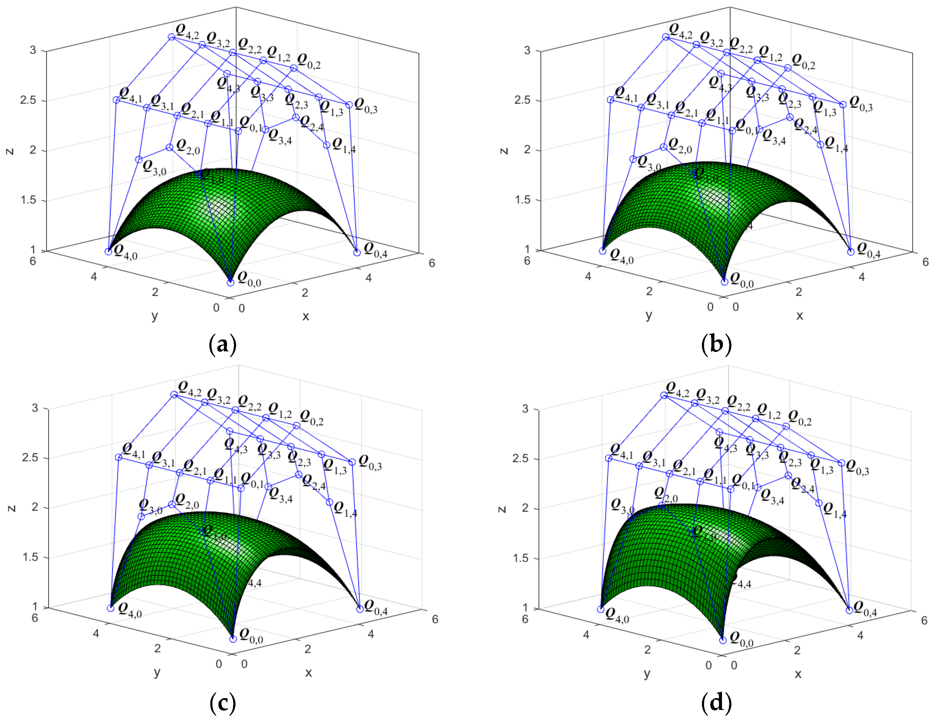
Given the control vertices $Q_{i,j}(i,j=0, 1, 2, 3, 4)$ and the shape parameters $\tilde{\Theta }$, the QGS-Ball surfaces $S(u,v;\Theta ,\tilde{\Theta })$ move in the same direction as the control vertices $Q_{i,0},$ $Q_{i,1}, Q_{i,2}, Q_{i,3}, Q_{i,4}$ by altering the shape parameters $\Theta$, that is, the shape parameters $\Theta$ affect the local surface shape around the control vertices $Q_{i,0}, Q_{i,1}, Q_{i,2}, Q_{i,3}, Q_{i,4}$. In addition, the shape of borderline curves $S(u,0;\Theta ,\tilde{\Theta })$ and $S(u,1;\Theta ,\tilde{\Theta })$ is changed, while the shape of borderline curves $S(0,v;\Theta ,\tilde{\Theta })$ and $S(1,v;\Theta ,\tilde{\Theta })$ is not changed (see Figure 10).

(2)

Given the control vertices $Q_{i,j}(i,j=0, 1, 2, 3, 4)$ and the shape parameters $\Theta$, the QGS-Ball surfaces $S(u,v;\Theta ,\tilde{\Theta })$ move in the same direction as the control vertices $Q_{0,j},$ $Q_{1,j}, Q_{2,j}, Q_{3,j}, Q_{4,j}$ by altering the shape parameters $\tilde{\Theta }$, that is, the shape parameters $\tilde{\Theta }$ affect the local surface shape around the control vertices $Q_{0,j}, Q_{1,j}, Q_{2,j}, Q_{3,j}, Q_{4,j}$. In addition, the shape of borderline curves $S(0,v;\Theta ,\tilde{\Theta })$ and $S(1,v;\Theta ,\tilde{\Theta })$ is changed, while the shape of borderline curves $S(u,0;\Theta ,\tilde{\Theta })$ and $S(u,1;\Theta ,\tilde{\Theta })$ is not changed (see Figure 11).

(3)

Given the control vertices $Q_{i,j}(i,j=0, 1, 2, 3, 4)$, if the shape parameters $\Theta$ and $\tilde{\Theta }$ are increased (or decreased) at the same time, the QGS-Ball surfaces $S(u,v;\Theta ,\tilde{\Theta })$ will approach (or move far from) its control mesh.

Keeping the control vertices unchanged, Figure 10 and Figure 11 show the shape change of the QGS-Ball surface when altering ${\lambda }_1$ and ${\tilde{\lambda }}_1$, respectively. From Figure 10 and Figure 11, we conclude that the QGS-Ball surface approaches the control mesh in the same direction as the control vertices $Q_{1,0}, Q_{1,1}, Q_{1,2}, Q_{1,3}, Q_{1,4}$, and the shape of borderline curves $S(u,0;\Theta ,\tilde{\Theta })$ and $S(u,1;\Theta ,\tilde{\Theta })$ is changed when ${\lambda }_1$ is increased. The QGS-Ball surface approaches the control mesh in the same direction as the control vertices $Q_{0,1}, Q_{1,1}, Q_{2,1},$ $Q_{3,1}, Q_{4,1}$, and the shape of borderline curves $S(0,v;\Theta ,\tilde{\Theta })$ and $S(1,v;\Theta ,\tilde{\Theta })$ is changed when ${\tilde{\lambda }}_1$ is increased.

6. Conclusions

In this work, the QGS-Ball basis functions containing three shape parameters were firstly defined, and we discussed and proved their properties. Secondly, the QGS-Ball curves were constructed on the basis of the proposed basis functions, the expression and properties of QGS-Ball curves were given, and the impact of three shape parameters on the curve was discussed. Since complex curves cannot be generated by a single QGS-Ball curve, we further defined the CQGS-Ball curves and derived the geometric continuity conditions of G¹ and G² smooth joining of QGS-Ball curves. Finally, the QGS-Ball surfaces were proposed by tensor product method, and the effect of shape parameters on the surface was further studied. In general, the constructed QGS-Ball curves and surfaces have the following merits: (1) The QGS-Ball curves and surfaces have better global and local shape adjustability compared with the traditional quartic Said-Ball curves and surfaces. (2) The construction method of CQGS-Ball curves is simple and effective, and the G¹ and G² geometric joining conditions are prone to realization, which is suitable for complex product shape design. (3) The modeling examples show that the designers can easily modify the shape of curves and surfaces by changing the shape parameters in daily graphic design, thereby making the graphic expression more aesthetically pleasing.

The future research content can be considered from two aspects. One is that this paper only discusses the theory and properties of QGS-Ball curve and surface containing multiple shape parameters, and the construction, properties, and related algorithms of higher-order generalized Said-Ball curve and surface with multiple parameters are worthy of further study [26,27]. The second is that we can use the highly efficient and improved chameleon swarm algorithm (MCSA) in [28] to optimize the QGS-Ball curve and surface, so as to construct the ideal shape of the curve and surface.

References

- Barnhill, R.E.; Riesenfeld, R.F. Computer Aided Geometric Design; Academic Press: New York, NY, USA, 1974. [Google Scholar]
- Ball, A.A. CONSURF, Part 1: Introduction to the conic lofting title. Comput. Aided Des. 1974, 6, 243–249. [Google Scholar] [CrossRef]
- Ball, A.A. CONSURF, Part 2: Description of the algorithms. Comput. Aided Des. 1975, 7, 237–242. [Google Scholar] [CrossRef]
- Ball, A.A. CONSURF, Part 3: How the program is used. Comput. Aided Des. 1977, 9, 9–12. [Google Scholar] [CrossRef]
- Wang, G.J. Ball curve of high degree and its geometric properties. Appl. Math. J. Chin. Univ. 1987, 2, 126–140. [Google Scholar]
- Said, H.B. A generalized Ball curve and its recursive algorithm. ACM Trans. Graph. 1989, 8, 360–371. [Google Scholar] [CrossRef]
- Hu, S.M.; Wang, G.Z.; Jin, T.G. Properties of two types of generalized Ball curves. Comput. Aided Des. 1996, 28, 125–133. [Google Scholar] [CrossRef]
- Othman, W.A.M.; Goldman, R.N. The dual basis functions for the generalized Ball basis of odd degree. Comput. Aided Geom. Des. 1997, 14, 571–582. [Google Scholar] [CrossRef]
- Hu, Q.; Wang, G. Rational cubic/quartic Said-Ball conics. Appl. Math. J. Chin. Univ. 2011, 26, 198–212. [Google Scholar] [CrossRef]
- Wu, H.Y. Two new classes of generalized Ball curves. Acta Math. Appl. Sin. 2000, 23, 196–205. [Google Scholar]
- Wu, H.Y. Dual bases for a new family of generalized Ball bases. J. Comput. Math. 2004, 22, 79–88. [Google Scholar]
- Wang, C.W. Extension of cubic Ball curve. J. Eng. Graph. 2008, 29, 1003–1058. [Google Scholar]
- Yan, L.L.; Wu, G.G.; Liang, J.F. Generalized Ball curves of ninth degree. In Proceedings of the 2009 International Conference on Environmental Science and Information Application Technology, Wuhan, China, 4–5 July 2009; Volume 1, pp. 557–560. [Google Scholar]
- Wu, X.Q.; Han, X.L. Shape analysis of quartic Ball curve with shape parameter. Acta Math. Appl. Sin. 2011, 34, 671–682. [Google Scholar]
- Xiong, J.; Guo, Q.W. Generalized Said-Ball curves. J. Numer. Methods Comput. Appl. 2012, 33, 58–67. [Google Scholar]
- Xiong, J.; Guo, Q.W. Generalized Wang-Ball curves. J. Numer. Methods Comput. Appl. 2013, 34, 187–195. [Google Scholar]
- Cao, H.X.; Zheng, H.C.; Hu, G. Adjusting the energy of Ball surfaces by modifying unfixed control balls. Numer. Algorithms 2022, 89, 749–768. [Google Scholar] [CrossRef]
- Liu, H.Y.; Li, L.; Zhang, D.M. Quartic Ball curve with multiple shape parameters. J. Shandong Univ. 2011, 41, 23–28. [Google Scholar]
- Huang, C.L.; Huang, Y.D. Quartic Wang-Ball type curves and surfaces with two parameters. J. Hefei Univ. Tech. 2012, 35, 1436–1440. [Google Scholar]
- Wang, C.W.; Chen, H. Extension of quartic Said-Ball curve with two parameters. In Mechanics and Mechanical Engineering: Proceedings of the 2015 International Conference (MME2015); World Scientific: Singapore, 2016; pp. 543–552. [Google Scholar]
- Hu, G.; Luo, L.; Li, R.; Yang, C. Quartic generalized Ball surfaces with shape parameters and its continuity conditions. In Proceedings of the International Conference on Computer Science and Network Technology, Dalian, China, 21–22 October 2017; pp. 5–10. [Google Scholar]
- Hu, G.; Du, B. Ball Said-Ball curve: Construction and its geometric algorithms. Adv. Eng. Softw. 2022, 174, 103334. [Google Scholar] [CrossRef]
- Hu, G.; Zhu, X.N.; Wei, G.; Chang, C. An improved marine predators algorithm for shape optimization of developable Ball surfaces. Eng. Appl. Artif. Intel. 2021, 105, 104417. [Google Scholar] [CrossRef]
- Hu, G.S.; Wang, D.; Yu, A.M.; Zhou, Q.T. 2m+2 order Ball curve construction and its applications with shape parameters. J. Eng. Graph. 2009, 30, 69–79. [Google Scholar]
- Hu, G.; Li, M.; Wang, X.F.; Wei, G.; Chang, C.T. An enhanced manta ray foraging optimization algorithm for shape optimization of complex CCG-Ball curves. Knowl.-Based Syst. 2022, 240, 108071. [Google Scholar] [CrossRef]
- Ghomanjani, F.; Noeiaghdam, S. Application of Said Ball Curve for Solving Fractional Differential-Algebraic Equations. Mathematics 2021, 9, 1926. [Google Scholar] [CrossRef]
- Debnath, P.; Srivastava, H.M.; Chakraborty, K.; Kumam, P. Advances in Number Theory and Applied Analysis; World Scientific: Singapore, 2023. [Google Scholar]
- Hu, G.; Yang, R.; Qin, X.Q.; Wei, G. MCSA: Multi-strategy boosted chameleon-inspired optimization algorithm for engineering applications. Comput. Methods Appl. Mech. Eng. 2023, 403, 115676. [Google Scholar] [CrossRef]