Combined Micro-Structural Effects of Linearly Increasing Reynolds Number and Mean Inflow Velocity on Flow Fields with Mesh Independence Analysis in Non-Classical Framework

Abstract

The monolithic Eulerian formulation has widely been employed for solving numerically fluid–structure interaction (FSI) problems of finite structural displacement using the same mathematical variational formulation for fluid and structural dynamics. Recently, different physical features of fluid flow have been analyzed using this approach to such coupling problems by computing the classical benchmark solutions in a non-classical framework. Despite producing decent results, the analysis of micro-structural characteristics of fluid flow by applying the classical benchmark solutions still needs to be enhanced and extended further for such coupling problems. In this paper, the classical benchmark solutions have been enhanced and extended further for analyzing the combined micro-structural effects of linearly increasing Reynolds number $R_e$ and mean inflow velocity $\overline{U}$ on flow fields with mesh independence analysis by employing a monolithic Eulerian formulation in a non-classical framework. To this aim, the Cosserat fluids theory is taken into account for the present coupling problem by considering three micro-rotational degrees of freedom (dof) of fluid particles. The model equations of the proposed Cosserat fluid–structure interaction (CFSI) problem are derived using underlying laws of continuum mechanics. A numerical section presents the implementation of the benchmark problem with test examples followed by a detailed evaluation of the obtained results. The results obtained indicate that a uniform linear increase in Reynolds number $R_e$ and mean inflow velocity $\overline{U}$ produce the significant combined micro-structural effects on the micro-rotation velocity field $\mathsf{\omega }$, and this effect is found increasing on the increase of both parameters. This combined effect of increasing $R_e$ and $\overline{U}$ on the velocity field $u$ is also observed to be very significant in a sense that horizontal and vertical flow velocity profiles experience great variation by maintaining the same pattern on each increasing value of $R_e$ and $\overline{U}$ at any particular location in the computational domain. Further, the mesh independence analysis is employed to verify the convergence of obtained results. The study concludes that the linear increase in Reynolds number and mean inflow velocity affect micro-rotational velocity field significantly at the micro-structural level with mesh independence analysis. Finally, some future recommendations to enhance and extend the study with some of its limitations are presented.

1. Introduction

Numerous interesting real-life problems related to fluid dynamics involve the mutual interaction of fluid and solid structure, where fluid flow depends on the displacement of solid structure, which is in turn influenced by fluid dynamics. In computational modeling, such a setup is commonly known as a fluid–structure interaction (FSI) problem. Examples of FSI problems are of great importance in many real-life applications, such as engineering, bio-mechanics, cardiovascular system modeling [1,2,3,4,5,6,7,8], etc., and numerical simulations of such coupling problems play an important role in the understanding and prediction of FSI phenomena in all these fields of studies. In such problems, the effects of FSI become more significant and noticeable, particularly in the case when the dependence between the influence and response becomes stronger. These effects sometimes can be catastrophic, especially in a solid structure made up of materials susceptible to fatigue. In engineering studies, the first Tacoma Narrows Bridge (1940) is considered one of the most infamous examples of large-scale failure due to the heavy interaction of fluid (wind) and solid structure (bridge), as represented pictorially in Figure 1.

A typical FSI model includes equations governing the fluid dynamics and the motion of the elastic solid structure together with coupling conditions at the fluid–structure interface. To date, many numerical approaches have been developed to solve such FSI problems, and the consideration taken into account for the most effective and related approach strongly depends on the different characteristics of the proposed problem to be studied. The major classification of numerical approaches is based on the way coupling between fluid and solid structure takes place, the way the mesh is generated, and the way in which discretization is performed to obtain the final algebraic equations to be solved.

There is a wealth of literature available on the numerous numerical approaches for solving FSI problems inside a traditional classical framework. Some numerical approaches are known as monolithic [9,10,11,12], where fluid dynamics and structural dynamics are treated inside the same mathematical variational formulation. In recent years, from the modeling point of view, monolithic approaches have been adopted extensively for solving FSI problems in many different fields of engineering and applied sciences. Meanwhile, the development of monolithic solvers in the solution procedure for solving such coupled problems all at once is considered, in general, a very hard task and has received a lot of attention. The main advantage of using this approach is that the implicit interfacial conditions are inherently present in the solution procedure of the formulated mathematical framework, and a single discretization scheme can be applied to the proposed problem [13,14]. The monolithic approach has also the advantage of stability since the mutual influence of fluid and solid structure can be taken into account directly. This approach can potentially achieve the desired accuracy for a multidisciplinary problem under consideration by requiring substantially more resources and expertise in developing and maintaining such specialized code [11]. A more recent work devoted to monolithic approaches can be seen in [15,16,17,18,19,20,21,22,23,24,25,26,27,28], and a comprehensive review of the recent developments of robust monolithic FSI solvers can be found in [29]. Among them, a monolithic approach in an Eulerian frame [23,27] works like the fully Eulerian formulation [13,30]. This monolithic Eulerian approach is well adapted to FSI problems of finite structural displacement in physically deformed configurations. Further, this numerical approach works with velocities everywhere in the proposed problem domain, while the fully Eulerian formulation [13,30,31,32,33,34] prefers to work with velocities in fluid and displacement in solid domains, respectively. Finally for obtaining energy stability, it is suggested to update the solid structure with its own velocity and remesh the fluid domain at every time step [23,27].

In contrast, partitioned approaches solve fluid and solid structure sub-problems separately according to the numerical solver and mesh discretization using an iterative process so that the computation of the fluid flow solution does not affect the solid structure solution at the same computing time. It is not only used in the FSI but the idea can be applied to different problems and situations. Partitioned approaches are traditionally adopted in engineering applications since it is easy to combine available solvers for fluid and solid mechanical problems. The development of partitioned numerical approaches has been extensively studied in the literature [35,36,37,38,39,40,41,42,43,44,45,46,47], which contains fixed-point iterations [35,36,37], Newton-like methods [38,39,40], or optimization techniques [41,42,43]. In this approach, the interfacial conditions of fluid and solid structure are usually considered explicit, and the information is exchanged at the interface according to the coupling technique [48]. However, the challenge of this approach is to coordinate the disciplinary algorithms for achieving accurate and efficient FSI solutions with minimal code modification. Partitioned approaches are divided into one-way and two-way coupling approaches, while two-way coupling is further classified into weakly and strongly coupled approaches. An overview of monolithic and partitioned approaches of the FSI is given in Figure 2.

The arbitrary Lagrangian–Eulerian (ALE) is another well-known numerical approach for solving FSI problems by incorporating the material, spatial, and referential descriptions of fluid and solid structure domains, respectively. The ALE formulation is also known as the interface-tracking approach, which is a finite-element formulation in which the proposed computational system is not a priori fixed in space (Eulerian formulation) or attached to material (Lagrangian formulation). The ALE formulation is used to capture the interaction between fluid and solid in the FSI problems by combining the advantages of the Lagrangian and the Eulerian formulations, respectively. In the ALE, the fluid equations of the FSI problems are generally written over a moving mesh by following the solid structural displacement [49,50], usually used for thin solid structures, and considered the most efficient in the case of small displacement [8,51,52]. Further, the velocities and stresses are incorporated at the interface of fluid and solid structure, followed by the mapping of fluid equations back into the structural domain at every time march during simulations [10,53]. However, in the case of finite structural deformation, the ALE fails, which leads to heavy distortion of the fluid mesh [54,55]. On the other hand, the immersed boundary method (IBM) [56,57] is used to approximate fluid flow on a fixed non-moving computational mesh, while the presence of the solid structure is usually implemented in different ways [58]. This method is effective for shells in the fluid for which mathematical analysis is more advanced [59], but the numerical implementations for thick structures lag behind [60]. Further, the immersed boundary-lattice Boltzmann method (LBM) is another Eulerian–Lagrangian approach used for FSI simulations even in flexible boundary problems [61].

Recently, extensive literature has been attributed to the significant analysis of the micro-structural characteristics of fluid flow by employing a monolithic Eulerian formulation to FSI problems of finite structural deformation by computing the classical benchmark test in a non-classical classical framework [62]. Nevertheless, the study of the micro-structural characteristics of fluid flow using these classical benchmark test solutions still needs to be enhanced and extended further to analyze the combined effect of linearly increasing Reynolds number $R_e$ and mean inflow velocity $\overline{U}$ on flow velocity fields with mesh independence analysis at the micro-structural level in a non-classical framework.

The mathematical formulation of such non-classical FSI models is based on the consideration of a continuum as an oriented rigid particle having three additional micro-rotational degrees of freedom (dof). In such non-classical coupling models, the response of the solid structure to its displacement and micro-rotation are commonly characterized by a non-symmetric Cauchy stress tensor and couple stress tensor, respectively. To this aim, the Cosserat fluids theory [63] is considered to model FSI problems in a non-classical framework. This theory was then further applied to describe fluids with micro-structures [64,65,66] and recently for FSI applications in [67,68,69]. A detail of the mathematical modeling can be seen in [70].

In this paper, the classical benchmark solutions have been enhanced and extended further to analyze the combined effect of linearly increasing Reynolds number $R_e$ and mean inflow velocity $\overline{U}$ on flow velocity fields with mesh independence analysis at the micro-structural level by employing a monolithic Eulerian formulation to CFSI problems of finite deformation in a non-classical framework. The results of the present study are obtained by computing the prominent classical FSI test FLUSTRUK-FSI-3* using the most popular publicly available software FreeFEM++ [71], which is very famous among the research community of engineering studies for FEM simulations. More recent work in [72,73,74] is devoted to the requirement and implementation of this software for simulating a variety of multi-physics problems. The results of the present study indicate the significant effect of linearly increasing Reynolds number and mean inflow velocity at the micro-structural level in a non-classical framework.

Contribution of the Study

The problems involving the interaction of fluid and solid structure have always been very important and challenging in the literature. In such problems, different characteristics of fluid flow depending on structural displacement have been analyzed. There is a wealth of literature available on the analysis of these characteristics of fluid flow in a traditional classical framework, but the non-classical framework still requires the attention of researchers for this analysis.

The main contributions of the present study are briefly described as follows:

➢

Analysis of different micro-structural characteristics of fluid flow for FSI problem in a non-classical framework.

➢

Use of the Cosserat theory of fluids.

➢

Employing a monolithic Eulerian formulation for solving the coupling problem of finite deformation in a non-classical framework.

➢

Computation and validation of the results using the prominent classical benchmark FSI test FLUSTRUK-FSI-3*‘flow around a cylinder.

➢

Implementation of algorithmic description with FreeFEM ++.

➢

Verification of the convergence of the results using mesh independence analysis in a non-classical framework.

This paper is organized as follows:

➢

Section 2 presents the mathematical modeling of the CFSI problem to be studied. This section includes an overview of the fundamental notations for continuum description, and then the complete derivation of the governing equations for fluid and solid structure from conservation laws using constitutive relations in a monolithic Eulerian frame is presented.

➢

Section 3 presents a monolithic variational formulation of the governing CFSI model in the Eulerian frame.

➢

Section 4 presents the discretization schemes, where the semi-implicit and the finite-element method are used for discretizing time and space domains, respectively.

➢

Section 5 describes the description, configuration, boundary conditions, and initial conditions of the benchmark test problem.

➢

Section 6 discusses the results of the study obtained from computer simulations.

➢

Section 7 concludes the present study with some of its future developments.

2. Cosserat Fluid–Structure Interaction Modeling

This section details the mathematical modeling of the present Cosserat fluid–structure interaction (CFSI) problem, which includes an overview of the fundamental notations for continuum description and the complete derivation of the governing equations for fluid and solid structure from conservation laws in a monolithic Eulerian frame.

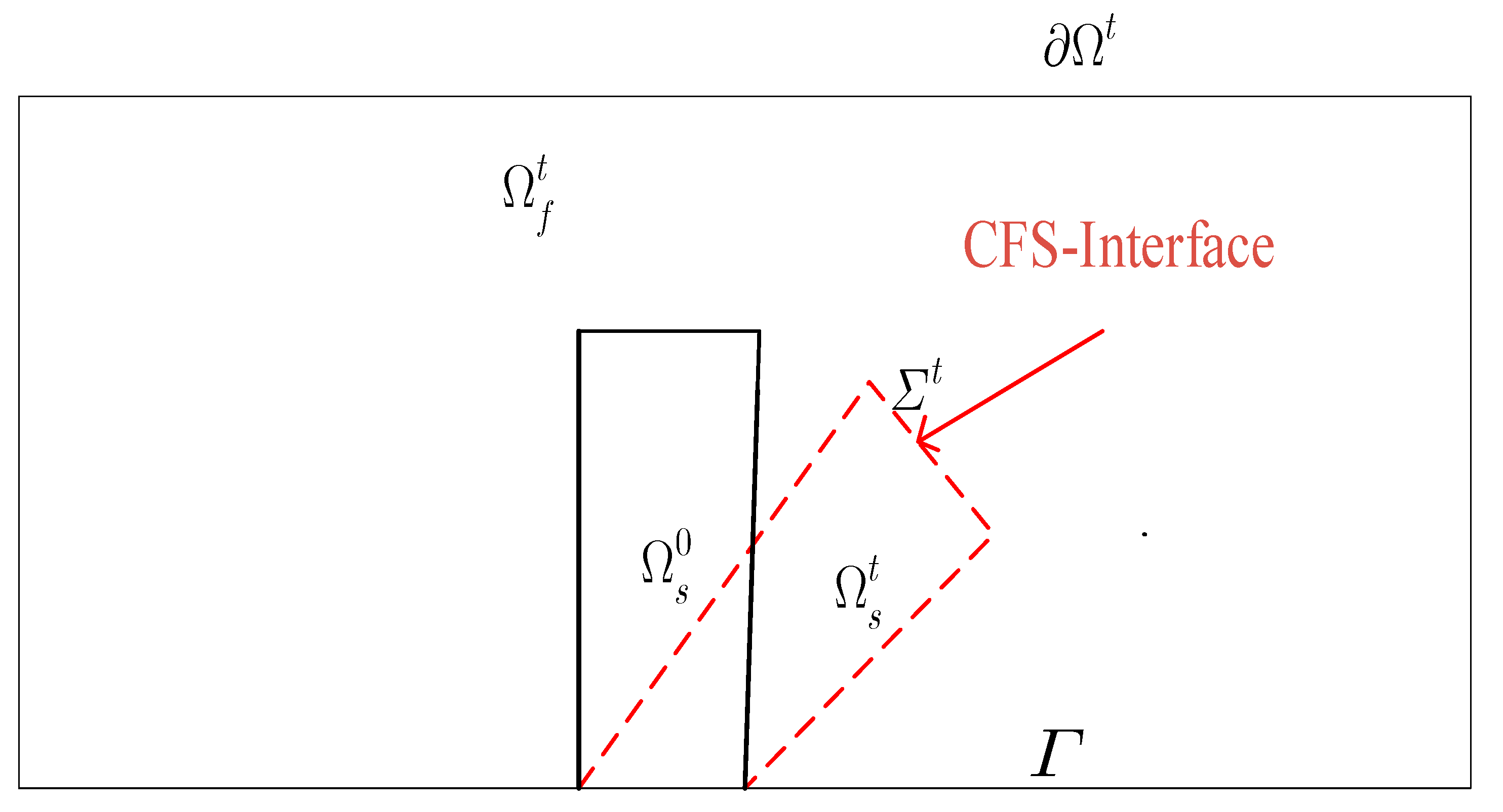
2.1. Fluid–Structure Interaction Problem Description

In the present CFSI problem, ${\Omega }^t$ is the time-dependent computational domain, which comprises fluid region ${\Omega }_f^t$ and solid region ${\Omega }_s^t$, respectively, such that ${\overline{\Omega }}^t={\overline{\Omega }}_f^t\cup \hspace{0.17em}{\overline{\Omega }}_s^t,{\Omega }_f^t\cap \hspace{0.17em}{\Omega }_s^t=\varnothing ,\hspace{0.17em}\forall t.$ The boundary of the computational domain and fluid–structure interface is denoted by $\partial {\Omega }^t$ and ${\Sigma }^t$, respectively, where ${\Sigma }^t={\overline{\Omega }}_f^t\cap {\overline{\Omega }}_s^t.$ The time-independent $\Gamma$ is taken as the part of the boundary of the computational domain $\partial {\Omega }^t$ on which either the solid structure clamps or it satisfies the ‘no-slip condition’ on the fluid. At $t=0$, the configuration is called the reference or undeformed configuration, and we assume that the system is at rest, i.e., $u_{f,s}={\mathsf{\omega }}_{f,s}=0$. The fluid is driven by an inflow boundary data on $\Gamma$, and the fluid’s stresses on the solid structure cause a deformation after some time $\forall t>0$ in the deformed or the present configuration. Further, fluid and solid domains are prescribed initially as ${\Omega }_f^0$ and ${\Omega }_s^0$, respectively, in this modeling. A schematic of this CFSI description can be seen in Figure 3.

2.2. Coupling Conditions

The coupling of fluid and solid problem is achieved by boundary conditions on the common interface ${\Sigma }^t$, which all stem from simple physical principles:

2.2.1. Kinematic Condition

The kinematic condition states that the velocity of fluid and the velocity of solid structure are continuous on the interface. This coupling condition stems from the observation that a viscous fluid sticks at the boundary. In Figure 3, the ‘no-slip condition’ defines that velocity of fluid at the interface must be the same as the velocity of solid (velocity due to its displacement). The ‘no-slip condition’ is generally termed the kinematic boundary condition. Mathematically,

$$u_f\left(x,t\right)=u_s\left(x,t\right) \mathrm{on} {\Sigma }^t,$$

(1)

The kinematic coupling condition has the type of the Dirichlet boundary condition, usually implied to the fluid problem when the boundary of the fluid domain is in motion.

2.2.2. Dynamic Condition

The dynamic coupling condition or stress continuity constraint relates to Newton’s third law of action and reaction: the stress exerted by fluid at the interface should be the same as the external force that acts on the solid.

$$n\cdot {\sigma }_f=n\cdot {\sigma }_s \mathrm{on} {\Sigma }^t,$$

(2)

The dynamic coupling condition is known as a Neumann boundary condition and usually implied to the solid problem.

2.2.3. Geometric Condition

The geometric coupling condition prevents the two sub-domains from separating or overlapping. This condition usually describes the domain motion along the interface. In this coupling condition, the path of a particle and its inverse are both continuous functions together with the condition that the normal velocities of fluid $n\cdot u_f$ and solid $n\cdot u_s$ are continuous along the common interface.

These three coupling conditions describe the interaction between fluid and solid structure in the multi-physics problems. All of these conditions can be described as boundary conditions for the sub-problems.

2.3. Field Variables and Tensors

In this study, the bold characters represent vectors and tensors, with some exceptions, such as $x,x^0\in {ℝ}^d,d=2$ or $3$. The standard notations used in the entire text are detailed in [10,37,62,75,76,77,78,79]. The following field variables in the present study are used:

➢

$X:{\Omega }^0\times \left(0,T\right)\mapsto {\Omega }^t:X\left(x^0,t\right)$ is the material location at time $t$ of $x^0$ (i.e., a material point at $x^0$ at $t=0$ is transported to $X$ at time $t$ by the motion).

➢

$d=X\left(x^0,t\right)-x^0$ is the displacement field.

➢

$u$ is the velocity field.

➢

$\mathsf{\omega }$ is the micro-rotation velocity field.

➢

$F_{ji}={\partial }_{x_i{}^0}{X}_j$ is the transposed deformation gradient tensor.

➢

$J=\det F$ is the Jacobian of deformation gradient tensor.

➢

$\rho \left(x,t\right)={\rho }_f{1}_{{\Omega }_f^t}\left(x,t\right)+{\rho }_s{1}_{{\Omega }_s^t}\left(x,t\right)$ is the density.

➢

$\sigma \left(x,t\right)={\sigma }_f{1}_{{\Omega }_f^t}\left(x,t\right)+{\sigma }_s{1}_{{\Omega }_s^t}\left(x,t\right)$ is the stress tensor.

In the above, ${\rho }_f$ and ${\sigma }_f$ are the density and the stress tensor in the fluid, while ${\rho }_s$ and ${\sigma }_s$ are the density and the stress tensor in the solid structure, respectively. The set function indicators $1_{{\Omega }_f^t}$ and $1_{{\Omega }_s^t}$ are used in numerical simulation [62].

Unless specified, all spatial derivatives in this mathematical modeling of the CFSI are taken with respect to $x\in {\Omega }^t$ and not w.r.t $x^0\in {\Omega }^0.$ If $\varphi$ is a function of $x=X\left(x^0,t\right)$ where $x^0\in {\Omega }^0,$ then

$${\nabla }_{x^0}\varphi =\left[{\partial }_{x_i{}^0}\varphi \right]=\left[{\partial }_{x_i{}^0}{X}_j{\partial }_{x_j}\varphi \right]=F^T\nabla \varphi .$$

(3)

In Equation (3) above, when $X$ is one-to-one and invertible, the relation between $F$ and $d$ can be seen as a function of $\left(x,t\right)$ instead of $\left(x^0,t\right)$, mathematically related as

$$F^T={\nabla }_{x^0}X={\nabla }_{x^0}\left(d+x^0\right)={\nabla }_{x^0}d+I=F^T\nabla d+I\hspace{1em}\hspace{1em}\Rightarrow F={\left(I-\nabla d\right)}^{-T}.$$

(4)

Further, the time derivatives of $\varphi$ are given by

$$D_t\varphi :=\frac{\partial }{\partial t}\varphi \left(X\left(x^0,t\right),t\right)={\partial }_t\varphi \left(x,t\right)+u\cdot \nabla \varphi \left(x,t\right),$$

(5)

where $D_t$ represents the material time derivative usually called total time derivative.

Finally, the deformation tensor and the micro-rotation strain tensor are, respectively, introduced as

$$Du=\left(L+L^T\right),$$

(6)

$$\mathit{\kappa }=\nabla \mathsf{\omega },$$

(7)

where $L=\nabla u$ is known as the velocity gradient tensor.

2.4. Conservation Laws

In the present study, conservation laws for fluid and solid structural material in a monolithic Eulerian formulation are given as

$$D_t\left(J\rho \right)=D_t\rho +\rho \nabla \cdot u=0. \mathrm{Conservation} \mathrm{of} \mathrm{mass}$$

(8)

$$\rho D_{t}u=\nabla \cdot {\sigma }_{s,f}+f. \mathrm{Conservation} \mathrm{of} \mathrm{momentum}$$

(9)

$$\rho {\rm I}{D}_t\mathsf{\omega }=\nabla \cdot C_f+\epsilon :{\sigma }_f+g. \mathrm{Conservation} \mathrm{of} \mathrm{angular} \mathrm{momentum}$$

(10)

where $f$ and $g$ are volume forces and volume couples, respectively, and $I$ is the coefficient of the micro-inertia. Further, incompressibility is employed as $J=1$, which leads to $\rho ={\rho }^0$.

The mathematical modeling of the CFSI system will be derived from these conservation laws by substituting the constitutive relation of materials into conservation laws, which are detailed in the remaining part of this section.

2.5. Constitutive Relations

In this work, the constitutive relations for fluid and solid structure are described as follow:

➢

For incompressible viscous Cosserat fluids:

$${\mathbf{\sigma }}_f=-p_{f}I+\mu \left(L+L^T\right)+{\mu }_r\left(L-L^T\right)-2{\mu }_r\mathit{\epsilon }\cdot \mathsf{\omega },$$

(11)

$$C_f=\alpha \left(tr\mathit{\kappa }\right)I+\beta \left(\kappa +{\mathit{\kappa }}^T\right)+\gamma \left(\mathit{\kappa }-{\mathit{\kappa }}^T\right),$$

(12)

where ${\mathsf{\sigma }}_f$, $C_f$, and $I$ are the non-symmetric stress tensor, the couple stress tensor, and the identity tensor, respectively. The pressure field and coefficient of dynamic viscosity are denoted by $p$ and $\mu$, respectively. The micro-viscosity coefficients and the Levi–Civita tensor are represented by ${\mu }_r$, $\alpha$, $\beta$,$\gamma$, and $\mathit{\epsilon }$.

➢

For an hyper-elastic incompressible solid structural material:

$${\sigma }_s=-p_{s}I+{\rho }_s{\partial }_F\Psi F^T,$$

(13)

where $\Psi$ is the Helmholtz potential, which, in the case of two-dimensional Mooney–Rivlin material [79], is defined as

$$\Psi \left(F\right)=c_{1}tr\left(F^{T}F\right)+c_2\left\{tr{\left(F^{T}F\right)}^2-t{r}^2\left(F^{T}F\right)\right\}.$$

(14)

2.6. Derivation of the Mooney–Rivlin Stress Tensor

For the derivation of the Mooney–Rivlin stress tensor ${\partial }_F\Psi F^T$, we use the fact that ${\partial }_F\mathrm{tr}\left(F^{T}F\right)=2F$ and ${\partial }_F\mathrm{tr}{\left(F^{T}F\right)}^2=4F{F}^{T}F.$ Hence Equation (14) becomes

$${\partial }_F\Psi =2c_{1}F+c_2\left\{4F{F}^{T}F-4\mathrm{tr}\left(F^{T}F\right)F\right\}.$$

(15)

Let $B=F{F}^T={\left(\left(I-\nabla d\right){\left(I-\nabla d\right)}^T\right)}^{-1},b=\det B\hspace{0.17em}\mathrm{and}\hspace{1em}c=\mathrm{tr}B.$ Then Equation (15) leads to

$${\partial }_F\Psi F^T=\left(2c_1-4c_{2}c\right)B+4c_2{B}^2.$$

(16)

Now apply Cayley–Hamilton theorem in Equation (16) above as

$$B^2=cB-bI.$$

(17)

Substituting Equation (17) into Equation (16), we get

$${\partial }_F\Psi F^T=2c_{1}B-4c_{2}bI=2c_{1}F{F}^T-4c_2\det \hspace{0.17em}(F{F}^T)I.$$

(18)

Again using the Cayley–Hamilton theorem in Equation (18) as

$$B=cI-b{B}^{-1}=cI-b\left(I-\nabla d-\nabla d^T+\nabla d\nabla d^T\right).$$

(19)

Now substituting Equation (19) into Equation (18), which leads to

$${\partial }_F\Psi F^T=\left\{2c_1(c-b)-4c_{2}b\right\}I+2c_{1}b\left(Dd-\nabla d\nabla d^T\right).$$

(20)

After simplifying and rearranging the terms in Equation (20) above, one arrives at

$${\partial }_F\Psi F^T=2c_1\det \left(F{F}^T\right)\left(Dd-\nabla d\nabla d^T\right)+\left\{2c_1\mathrm{tr}\left(F{F}^T\right)-\left(2c_1+4c_2\right)\det \left(F{F}^T\right)\right\}I.$$

(21)

Hence an incompressible two-dimensional Mooney–Rivlin material will have form for some ${\alpha }^{\prime }$

$${\partial }_F\Psi F^T=2c_1\left(Dd-\nabla d\nabla d^T\right)+{\alpha }^{\prime }I,$$

(22)

where ${\alpha }^{\prime }=\left\{2c_1\mathrm{tr}\left(F{F}^T\right)-\left(2c_1+4c_2\right)\det \left(F{F}^T\right)\right\}$ is some scalar function of structural material parameters $c_1$ and $c_2$.

2.7. Mathematical Formulation of Cosserat Fluids Theory

The governing model equations for Cosserat fluids as described in [70] can be derived by substituting the constitutive relations as given in Equations (11) and (12) into the equations of conservation laws (8)–(10) and by applying the prescribed boundary conditions, which leads to:

$$\nabla \cdot u=0,$$

(23)

$$\rho \left(\frac{\partial u}{\partial t}+u\cdot \nabla u\right)=-\nabla p+\left(\mu +{\mu }_r\right)\Delta u+2{\mu }_r\left(\nabla \times \mathsf{\omega }\right)+f,$$

(24)

$$\rho \left(I\frac{\partial \omega }{\partial t}+Iu\cdot \nabla \omega \right)=\lambda \Delta \omega +{\lambda }_0\nabla \left(\nabla \cdot \omega \right)-4{\mu }_r\omega +2{\mu }_r(\nabla \times u)+g,$$

(25)

where $\lambda =\beta +\gamma$ and ${\lambda }_0=\alpha +\beta -\gamma$ are positive material parameters.

Based on the above mathematical modeling of the present CFSI problem, the variational formulation and discretization schemes of the proposed model are described in the next sections.

3. Variational Formulation

Considering only homogeneous boundary conditions on $\Gamma \subset \partial {\Omega }^t$, i.e., clamped or ‘no-slip’, and homogeneous Neumann conditions on $\partial {\Omega }^t\backslash \Gamma$ for the proposed CFSI model, the final two-dimensional monolithic variational formulation in the Eulerian frame is:

Find $\left(u,\mathsf{\omega },p,d,{\Omega }_f^t,{\Omega }_s^t\right)$ with $u{|}_{\Gamma }=0$ and $\mathsf{\omega }{|}_{\Gamma }=0,$ given ${\Omega }_f^0$, ${\Omega }_s^0$ and $d$, $u$ and $\mathsf{\omega }$ at $t=0$, such that

$$\begin{array}{l}\begin{array}{c}{\displaystyle \underset{{\Omega }_f\cup \hspace{0.17em}{\Omega }_s}{\int }\{\rho D_{t}u\cdot \tilde{u}-p\nabla \cdot \tilde{u}-\tilde{p}\nabla \cdot u+(\mu +{\mu }_r)Du:D\tilde{u}-2{\mu }_r(\nabla \times \omega )\cdot \tilde{u}\}}d\Omega \hspace{1em}\\ +{\displaystyle \underset{{\Omega }_s}{\int }{c}_3(Dd-}\nabla d\nabla d^T):D\tilde{u}d{\Omega }_s={\displaystyle \underset{{\Omega }_f\cup {\Omega }_s}{\int }f\cdot \tilde{u}}d\Omega ,\end{array}\hspace{1em}\\ \hspace{1em}\hspace{1em}\end{array}$$

(26)

$$\begin{array}{l}{\displaystyle \underset{{\Omega }_f\hspace{0.17em}\cup \hspace{0.17em}\hspace{0.17em}{\Omega }_s}{\int }\{\rho D_t\left(I\mathsf{\omega }\right)\cdot \tilde{\mathsf{\omega }}+\lambda \left(\nabla \mathsf{\omega }:\nabla \tilde{\mathsf{\omega }}\right)-{\lambda }_0\nabla \left(\nabla \cdot \mathsf{\omega }\right)\cdot \tilde{\mathsf{\omega }}+4{\mu }_r\mathsf{\omega }\cdot \tilde{\mathsf{\omega }}}-2{\mu }_r\left(\nabla \times u\right)\cdot \tilde{\mathsf{\omega }}\}d\Omega \\ ={\displaystyle \underset{{\Omega }_f\cup \hspace{0.17em}\hspace{0.17em}{\Omega }_s}{\int }g\cdot \hspace{0.17em}\tilde{\mathsf{\omega }}}d\Omega ,\end{array}$$

(27)

for all $(\tilde{u},\tilde{\mathsf{\omega }},\tilde{p})$ with $\tilde{u}{|}_{\Gamma }=0$ and $\tilde{\mathsf{\omega }}{|}_{\Gamma }=0$.

In the above variational formulation, $\hspace{0.17em}{\Omega }_f^t$ and $\hspace{0.17em}{\Omega }_s^t$ are defined incrementally by

$$\frac{d{\rm X}}{d\tau }=u({\rm X}(\tau ),\tau ),\hspace{1em}$$

(28)

where

$$\hspace{0.17em}{\rm X}(t)\in {\Omega }_r^t\Rightarrow {\rm X}(\tau )\in {\Omega }_r^{\tau }\hspace{0.17em}\hspace{1em}\forall \tau \in (0,T),\hspace{1em}r=s,f.$$

(29)

Finally, the notations $B:C=tr(B^{T}C)$ and $c_3={\rho }_s{c}_1$ are also used in the derivation of the proposed variational formulation.

4. Discretization

This section is devoted to discretization schemes of variational Formulations (26) and (27) to approximate the CFSI problem in a non-classical framework. To this aim, a semi-implicit scheme for time and finite-element method for space domains are employed, respectively.

4.1. Monolithic Semi-Implicit Time Discretization

During the numerical simulations of this study, we consider the time $t\in \left[0,T\right]$ as simulation time, where $T$ denotes the total time. To run the simulation, the interval $\left[0,T\right]$ $\delta t=\frac{T}{N}$ such that $t=n\delta t$ where $n=0,1,\cdots ,N.$ It is naturally used the fact that

$${\displaystyle \underset{{\Omega }^t}{\int }\left(Dd-\nabla d\nabla d^T\right):D\tilde{u}\approx {\displaystyle \underset{{\Omega }^n}{\int }\left(D{d}^{n+1}-\nabla d^{n+1}\nabla d^{n+1}{}^{{}^T}\right):D\tilde{u}}}.$$

(30)

with $d^{n+1}=d^n+\delta t{u}^{n+1}.$ Hence

$$Dd-\nabla d\nabla d^T\approx D{d}^n-\nabla d^n{d}^n{}^{{}^T}+\delta t\left(D{u}^{n+1}-\nabla u^{n+1}{d}^n{}^{{}^T}-\nabla d^n\nabla u^{n+1}{}^{{}^T}\right)\hspace{0.17em}+o\left(\delta t\right).$$

(31)

We now consider the fact that, if ${{\rm X}}^n$ is a first-order approximation of ${\rm X}\left(t^{n+1}-\delta t\right)$ defined by $\dot{{\rm X}}=u\left({\rm X}\left(\tau \right),\tau \right),\hspace{0.17em}{\rm X}\left(t^{n+1}\right)=x,$ where ${\rm X}\left(t^{n+1}\right)=x$ such that ${{\rm X}}^n\left(x\right)=x-\delta t{u}^n\left(x\right),$ then a first-order in time approximation for the CFSI system based on its variational Formulation (26) and (27), leads to:

Find $\left(u^{n+1},{\mathsf{\omega }}^{n+1},p^{n+1}\right)$, ${\Omega }_f^{n+1}$ and ${\Omega }_s^{n+1}$ such that with $u^{n+1}{|}_{\Gamma }=0,$ ${\mathsf{\omega }}^{n+1}{|}_{\Gamma }=0$ and ${\Omega }^{n+1}={\Omega }_f^{n+1}\cup {\Omega }_s^{n+1},$ $\forall$$\left(\tilde{u},\tilde{\mathsf{\omega }},\hspace{0.17em}\tilde{p}\right)$ with $\tilde{u}{|}_{\Gamma }=0$ and $\tilde{\mathsf{\omega }}{|}_{\Gamma }=0,$ the following holds:

$$\begin{array}{l}{\displaystyle \underset{{\Omega }_f^n\cup {\Omega }_s^n}{\int }\{\left({\rho }^n\hspace{0.17em}\frac{u^{n+1}-u^{n}o{{\rm X}}^n}{\delta t}\right)}\cdot \tilde{u}-p^{n+1}\nabla \cdot \tilde{u}-\tilde{p}\nabla \cdot u^{n+1}+\left(\mu +{\mu }_r\right)D{u}^{n+1}:D\tilde{u}-2{\mu }_r\left(\nabla \times {\omega }^{n+1}\right)\cdot \tilde{u}\}d{\Omega }^n\\ +{\displaystyle \underset{{\Omega }_s^n}{\int }{c}_3[\{D{d}^n-\nabla d^n{}^{{}^T}\nabla d^n}+\delta t\left(D{u}^{n+1}-\nabla u^{n+1}\nabla d^n{}^{{}^T}-\nabla d^n\nabla u^{n+1}{}^{{}^T}\right)\}:D\tilde{u}]d{\Omega }_s^n={\displaystyle \underset{{\Omega }_f^n\cup {\Omega }_s^n}{\int }f}\cdot \hspace{0.17em}\tilde{u}d{\Omega }^n,\end{array}$$

(32)

$$\begin{array}{l}{\displaystyle \underset{{\Omega }_f^n\cup {\Omega }_s^n}{\int }\{{\rho }^n{I}^n\left(\frac{{\mathsf{\omega }}^{n+1}-{\mathsf{\omega }}^{n}o{{\rm X}}^{{}^n}}{\delta t}\right)}\cdot \tilde{\mathsf{\omega }}+\lambda \left(\nabla {\mathsf{\omega }}^{n+1}:\nabla \tilde{\mathsf{\omega }}\right)-{\lambda }_0\nabla \left(\nabla \cdot {\mathsf{\omega }}^{n+1}\right)\cdot \tilde{\mathsf{\omega }}+4{\mu }_r{\mathsf{\omega }}^{n+1}\cdot \tilde{\mathsf{\omega }}-2{\mu }_r\left(\nabla \times u^{n+1}\right)\cdot \tilde{\mathsf{\omega }}\}d{\Omega }^n\\ ={\displaystyle \underset{{\Omega }_f^n\cup {\Omega }_s^n}{\int }g}\cdot \tilde{\mathsf{\omega }}d{\Omega }^n.\end{array}$$

(33)

Then, update $d$ by

$$d^{n+1}=d^{n}o{{\rm X}}^n+\delta t{u}^{n+1},$$

(34)

and ${\Omega }_r^n$ by

$${\Omega }_r^{n+1}=\left\{x+\delta t{u}^{n+1}\left(x\right):x\in {\Omega }_r^n\right\},$$

(35)

where $r=s,f$.

4.2. Monolithic Finite Elements Space-Discretization

In this discretization scheme, the finite-element functional spaces for the displacement field, velocity field, micro-rotation field, and pressure field are represented as $V_h$, $W_h$ and $Q_h$, respectively. In this consideration, the triangulation ${\Im }_h^0$ lies in the initial domain ${\Omega }^0$, where quadratic elements are used for displacements, translational, micro-rotational velocity fields, and linear elements for pressure field, respectively. Further different preesures are taken into consideration in fluid and solid structural domains, respectively, because of the discontinuity of pressure at the fluid–structure interface, which results in $Q_h$, a piecewise linear function on the triangulation and continuous in ${\Omega }_r^{n+1},r=s,f$. A small penalization parameter $\zeta \ll 1$ is taken into account for imposing uniqueness of the pressure when a linear solver is required for the solution. So, at each time step, the space-discretization with FEM, leads to:

Find $\left(u_h^{n+1},{\mathsf{\omega }}_h^{n+1},p_h^{n+1}\right):\forall \hspace{0.17em}\left({\tilde{u}}_h,{\tilde{\mathsf{\omega }}}_h,{\tilde{p}}_h\right)\in \left(V_{0h},W_{0h},Q_h\right)$ with $V_{0h}{|}_{\Gamma }=0$ and $W_{0h}{|}_{\Gamma }=0$ are sub-spaces of $V_h$ and $W_h$, such that

$$\begin{array}{c}\begin{array}{l}{\displaystyle \underset{{\Omega }_f^n\cup {\Omega }_s^n}{\int }\{\left({\rho }^n\frac{u_h{}^{n+1}-u_h{}^{n}o{{\rm X}}^n}{\delta t}\right)\cdot {\tilde{u}}_h-p_h{}^{n+1}\nabla \cdot {\tilde{u}}_h-{\tilde{p}}_h\nabla \cdot u_h^{n+1}+\left(\mu +{\mu }_r\right)D{u}_h^{n+1}:D{\tilde{u}}_h-2{\mu }_r\left(\nabla \times {\omega }_h{}^{n+1}\right)\cdot {\tilde{u}}_h\}{\Omega }^n}\\ +{\displaystyle \underset{{\Omega }_s^n}{\int }{c}_3}\left[\left\{D{d}_h^n-\nabla d_h^{n^T}\nabla d_h^n+\delta t\left(D{u}_h^{n+1}-\nabla u_h^{n+1}\nabla d_h^{n^T}-\nabla d_h^n\nabla u_h^{n+1^T}\right)\right\}:D{\tilde{u}}_h\right]d{\Omega }_s^n+{\displaystyle \underset{{\Omega }_f^n\cup {\Omega }_s^n}{\int }\zeta p_h{\tilde{p}}_{h}d{\Omega }^n={\displaystyle \underset{{\Omega }_f^n\cup {\Omega }_s^n}{\int }f\hspace{0.17em}\cdot {\tilde{u}}_{h}d{\Omega }^n,}}\end{array}\\ \end{array}$$

(36)

$$\begin{array}{l}{\displaystyle \underset{{\Omega }_f^n\cup \hspace{0.17em}{\Omega }_s^n}{\int }\{{\rho }^n{I}^n\left(\frac{{\mathsf{\omega }}_h^{n+1}-{\mathsf{\omega }}_h^{n}o{{\rm X}}^n}{\delta t}\right)\cdot {\tilde{\mathsf{\omega }}}_h+\lambda \left(\nabla {\mathsf{\omega }}_h^{n+1}:\nabla {\tilde{\mathsf{\omega }}}_h\right)-{\lambda }_0\nabla \left(\nabla \cdot {\mathsf{\omega }}_h^{n+1}\right)\cdot {\tilde{\mathsf{\omega }}}_h}+4{\mu }_r{\mathsf{\omega }}_h^{n+1}\cdot {\tilde{\mathsf{\omega }}}_h-2{\mu }_r\left(\nabla \times u_h^{n+1}\right)\cdot {\tilde{\mathsf{\omega }}}_h\}d{\Omega }^n\\ \hspace{1em}\hspace{1em}\hspace{1em}=\hspace{0.17em}{\displaystyle \underset{{\Omega }_f^n\cup \hspace{0.17em}{\Omega }_s^n}{\int }g\hspace{0.17em}\cdot {\tilde{\mathsf{\omega }}}_{h}d{\Omega }^n.}\end{array}$$

(37)

4.3. Finite-Element Mesh Updating Strategy

In order to update the finite-element triangulation during CFSI simulation at each vertex $\hspace{0.17em}{q}_i^n$ of the triangle $T_h\in {\Im }_h^n$, the vertex is moved to a new position by

$$q_i^{n+1}:=q_i^n+\delta t{u}_h^{n+1}.$$

(38)

Let $d_i^n:=d^n\left(q_i\right),$ then

$$d^{n}o{{\rm X}}^n\left(q_i^{n+1}\right)=d^n\left(q_i^n+\delta t{u}_h^{n+1}-\delta t{u}_h^{n+1}\right)=d^n\left(q_i^n\right).$$

(39)

In the above, it implies that the displacement vector of vertices $d_h^n$ can be copied to $d_i^{n+1}$ plus with the addition of $\delta t{u}_h^{n+1}\left(q_i^n\right)$ in order to obtain $d_h^{n+1}$, as

$$d_h^{n+1}=d_h^{n}o{{\rm X}}^n+\delta t{u}_h^{n+1}\left(q_i^n\right)=d_h^n+\delta t{u}_h^{n+1}\left(q_i^n\right).$$

(40)

Lastly, the solution of the Laplace equation $-\Delta \tilde{u}=0$(i.e.,$\tilde{u}$) is used to move the vertices in the fluid and $\tilde{u}=u$ on the CFSI interface $\Sigma$ and zero on the other boundaries. Moving the vertices of each triangle $T_h\in {\Im }_h^n$ by the above-given procedure gives a new finite-element triangulation ${\Im }_h^{n+1}$. (Note: Solving a Laplace equation in the fluid part with Dirichlet conditions equal to the velocity of the fluid–structure interface).

5. Numerical Tests

In this section, the numerical results of the present study are obtained by computing a prominent classical benchmark FSI test problem FLUSTRUK-FSI-3* ‘flow around a cylinder’. The selection of this benchmark test is based on its relevance to the proposed coupling problem and reliability for achieving the desired accuracy in the results. These results are then utilized to analyze the combined effect of linearly increasing Reynolds number $R_e$ and mean inflow velocity $\overline{U}$ on flow velocity fields at the micro-structural level with mesh independence analysis to verify the convergence of the results obtained in a non-classical framework.

The present benchmark test was first proposed and studied by [80] and then by [23,30,81], respectively, in a classical framework, and more recently by [62] in a non-classical framework.

5.1. Description of Benchmark Test

A beam, shaped like a rectangular flag, made of an hyper-elastic incompressible Mooney–Rivlin material, is attached behind a hard fixed cylinder in the computational rectangular domain; the flow enters from the left and is free to leave on the right. The dimensions of a rectangular flag and the computational domain are given as:

Dimension of rectangular flag: $\left[0,l\right]\times \left[0,h\right]$

Dimension of the computational domain: $\left[0,L\right]\times \left[0,H\right]$

5.2. Configuration, Boundary, and Initial Conditions

The configuration, boundary conditions, and initial conditions for the present benchmark test FLUSTRUK-FSI-3* are described in

Table 1. Configuration, boundary conditions, and initial conditions for the benchmark test.

Configuration	Boundary Conditions	Initial Conditions
The dimensions for computational domain: length $L=2.5 \mathrm{m}$, height $H=0.41 \mathrm{m}$. Elastic solid medium (like rectangular flag) dimensions: length $l=0.35 \mathrm{m}$, height $h=0.02 \mathrm{m}$. The left bottom corner is at $\left(0,0\right)$. The point $\left(0.2 \mathrm{m},0.2 \mathrm{m}\right)$ and $r=0.05 \mathrm{m}$ are center and radius of a cylinder, respectively. All above set cylinder slightly below the symmetry line of the computational domain.	Top and bottom boundaries of the computational domain satisfies the ‘no-slip condition’. A parabolic profile is prescribed at the left inlet, i.e., $u_f\left(0,y\right)=\overline{U}\left(\frac{6y\left(H-y\right)}{H^2}\right),$ where $\overline{U}$ is mean inflow velocity with flux $\overline{U}H$. The zero-stress $\sigma \cdot n=0$ is employed at the right outlet using ‘do-nothing ‘approach. For solid medium we consider no external forces.	All flow velocities and solid medium displacements are considered zero.

, as suggested in [23,30,62]:

Finally, additional material constants used in the numerical test are listed in

Table 2. Material constants for numerical test.

Material Constant	Value
${\rho }_f={\rho }_s$	${10}^3 {\mathrm{kgm}}^{-3}$
${\nu }_f$	${10}^{-3} {\mathrm{m}}^2{\mathrm{s}}^{-1}$
$c_1$	${10}^6 {\mathrm{kgm}}^{-1}{\mathrm{s}}^{-1}$

.

6. Results and Discussion

In this section, the results of the study are used to analyze the combined effect of linearly increasing Reynolds number $R_e$ and mean inflow velocity $\overline{U}$ on flow velocity fields significantly at the micro-structural level by validating the results in a non-classical framework with classical solutions present in literature. Further, the mesh independence analysis is employed to verify the convergence of the results obtained in this study and demonstrated for flow velocity fields.

6.1. Validation of Benchmark Test

The present study is a further extension of [62], which has been used to enhance the results of the proposed mathematical modeling obtained by computing the classical benchmark test FLUSTRUK-FSI-3* for the analysis of micro-structural characteristics of fluid flow in a non-classical framework. To strengthen the obtained results, the present classical benchmark is validated by comparing the results with classical benchmark solutions of the literature according to the standards for validation in CFD [82]. For validation, the flow needs to develop a Karman vortex street during computer simulation around $t\sim 2\mathrm{s}$. The validation is based on the comparison of horizontal and vertical displacements of the flagella end tip used for computing the frequency and the amplitude of oscillations, as shown in Figure 4 and Figure 5, respectively. The results are obtained with a mesh of $2199$ vertices and a uniform time-step size of $0.005 \mathrm{s}.$ The frequency $4.5 {\mathrm{s}}^{-1}$ and the amplitude $0.03$ validate the benchmark test FLUSTRUK-FSI-3* with classical solutions, as present in [23]. In this computation, the notations ${\mu }_c$ and ${\mu }_r$ denote the coefficient of micro-inertia and micro-rotational viscosity, respectively, while $\lambda$ combines the shear spin and rotational spin viscosities in the numerical simulation. Further, this validation is performed by taking Reynolds number $R_e=200$ and mean inflow velocity $\overline{U}=2$, and both are related linearly.

Finally, the number of vertices in the mesh, the frequency, the amplitude, and the time step size of the present study are compared with the values those are given in [23,30] for the proposed benchmark test, as listed below in

Table 3. Comparison of numerical data for validation with different studies.

Computation of FSI Tests	No. of Vertices	$\mathbf{Frequency} {\mathbf{s}}^{-1}$	Amplitude	$\mathbf{Time}-\mathbf{Step} \mathbf{Size} \mathbf{s}$
Present Study	2199	4.5	0.03	0.005
Hecht and Pironneau (2017)	2200	5.4	0.03	0.005
Dunne and Rannacher (2006)	2082	0.02226	1.92	0.005

.

After validation of the benchmark test, the results obtained are used to study the combined effects of linearly increasing Reynolds number and mean inflow velocity for analyzing the micro-structural characteristics of fluid flow with mesh independence analysis.

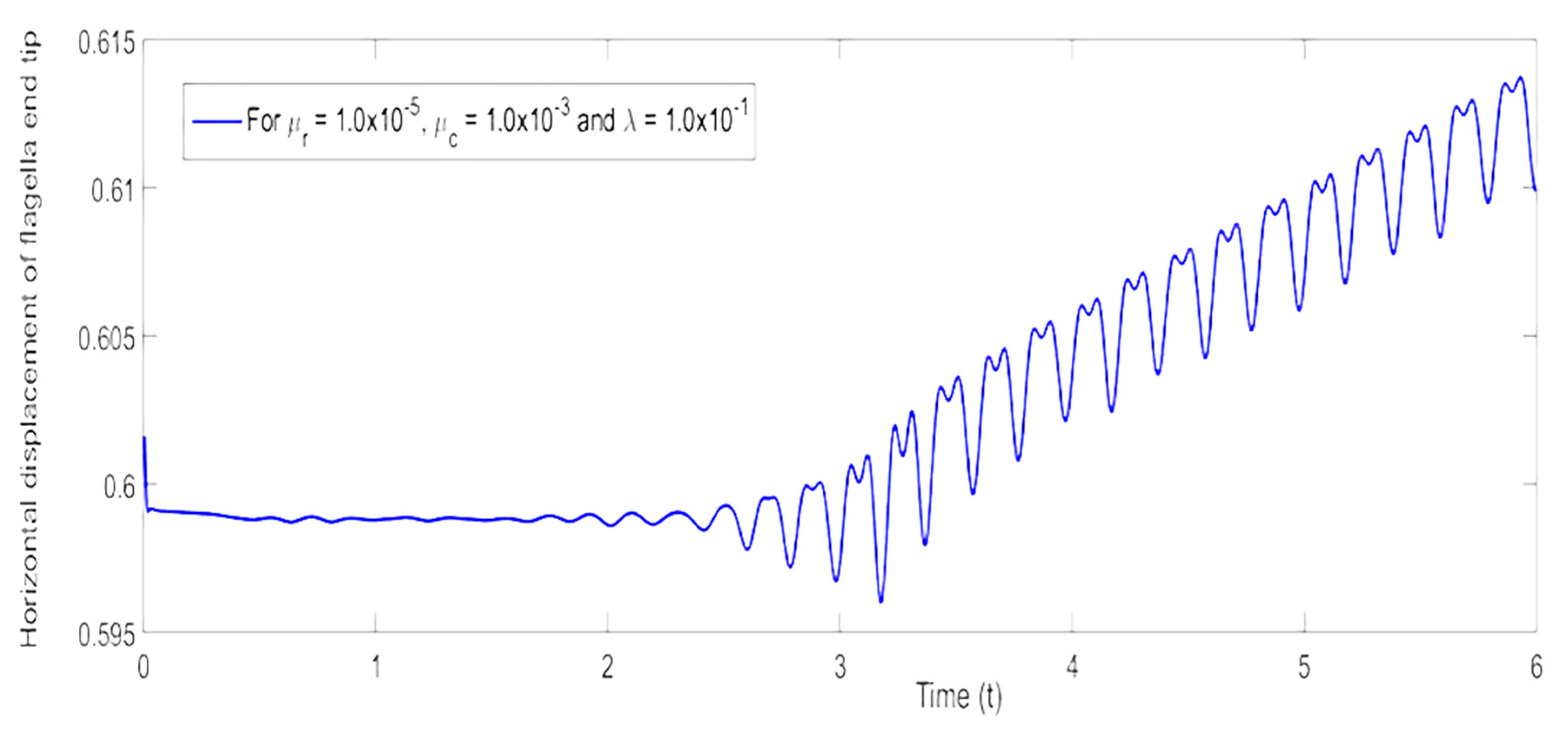
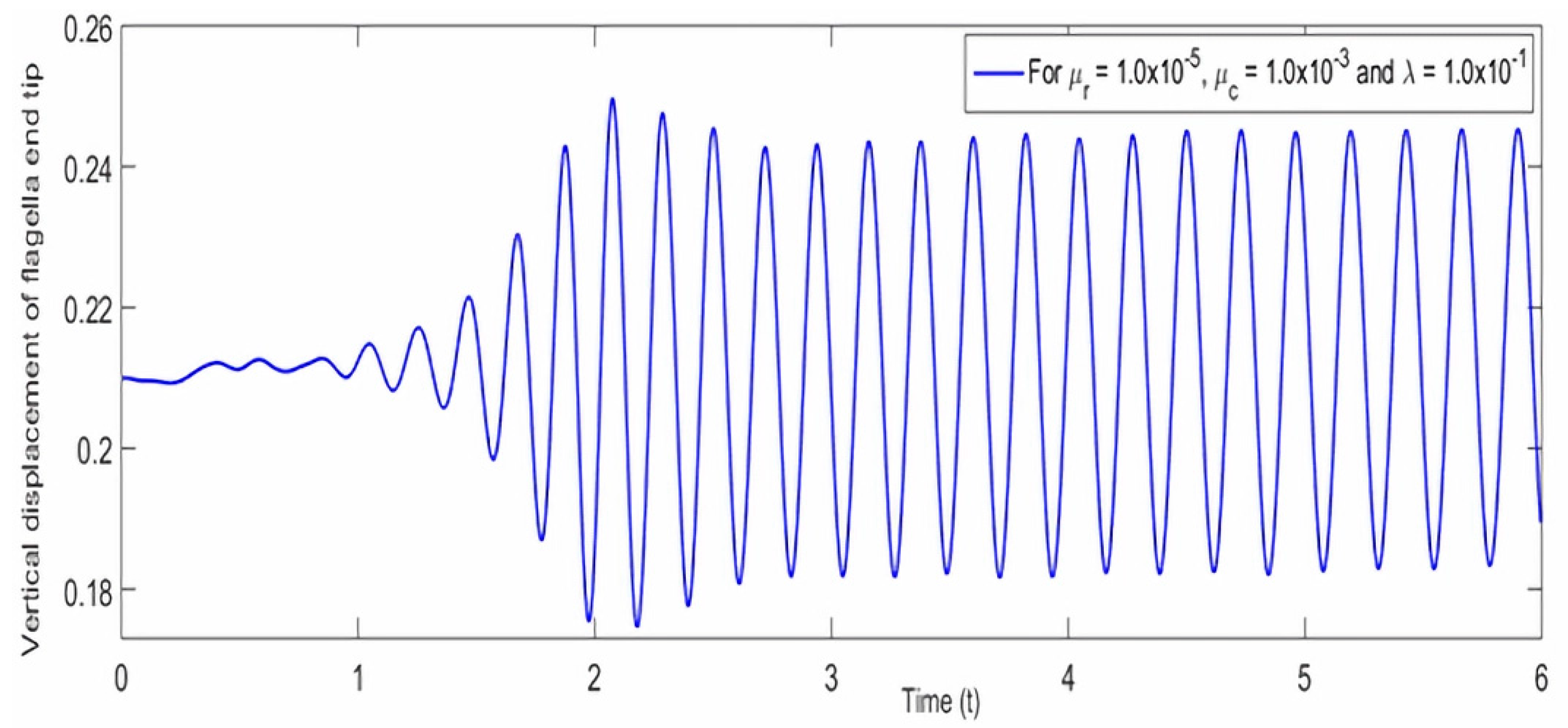
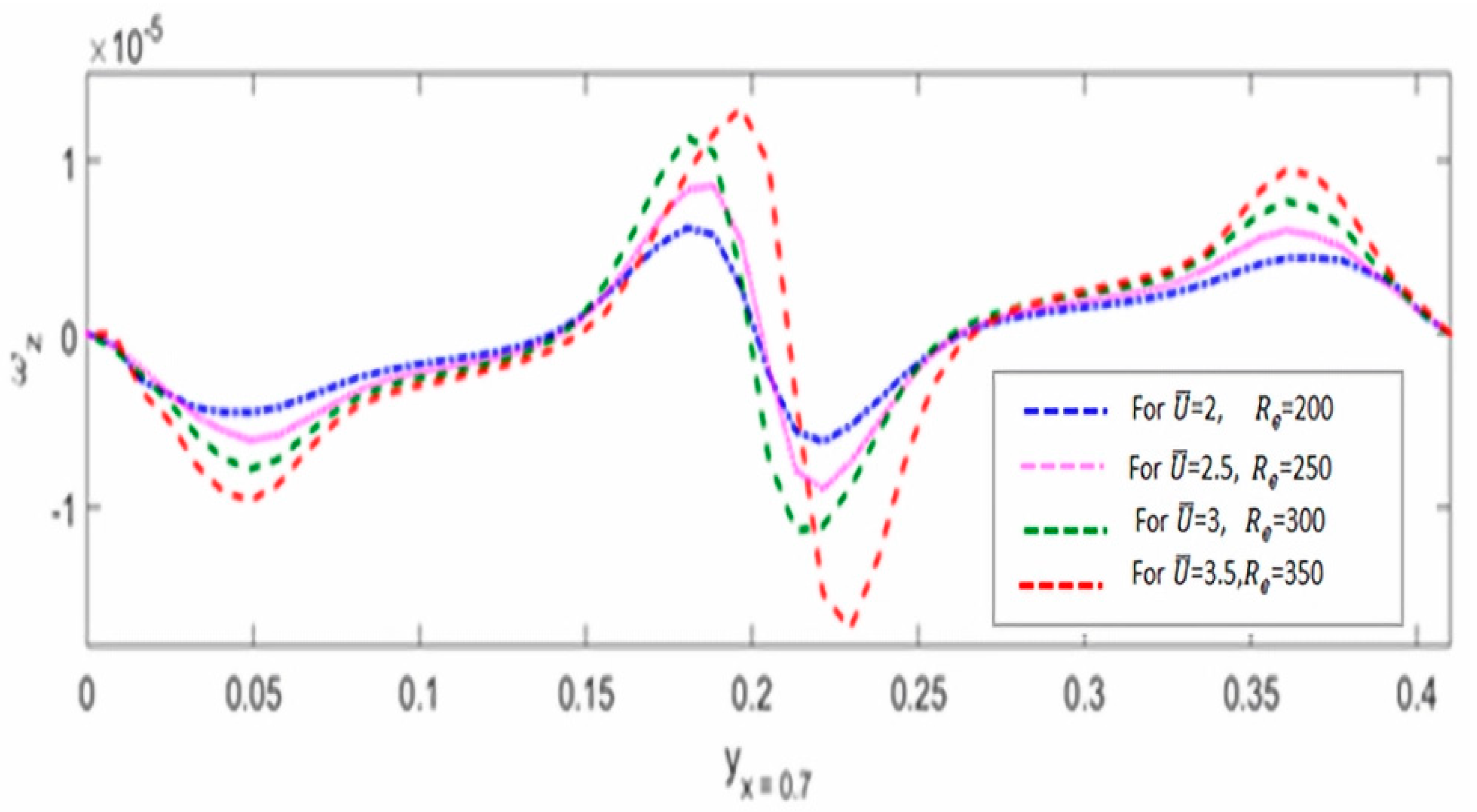
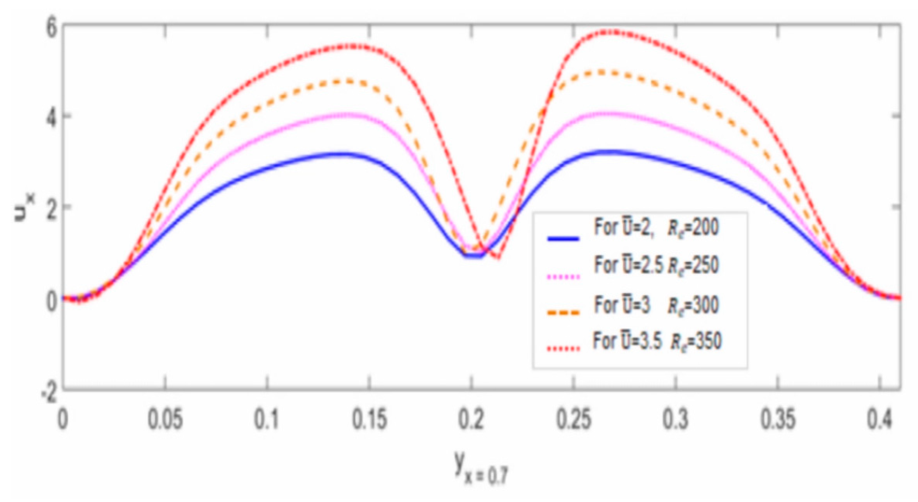
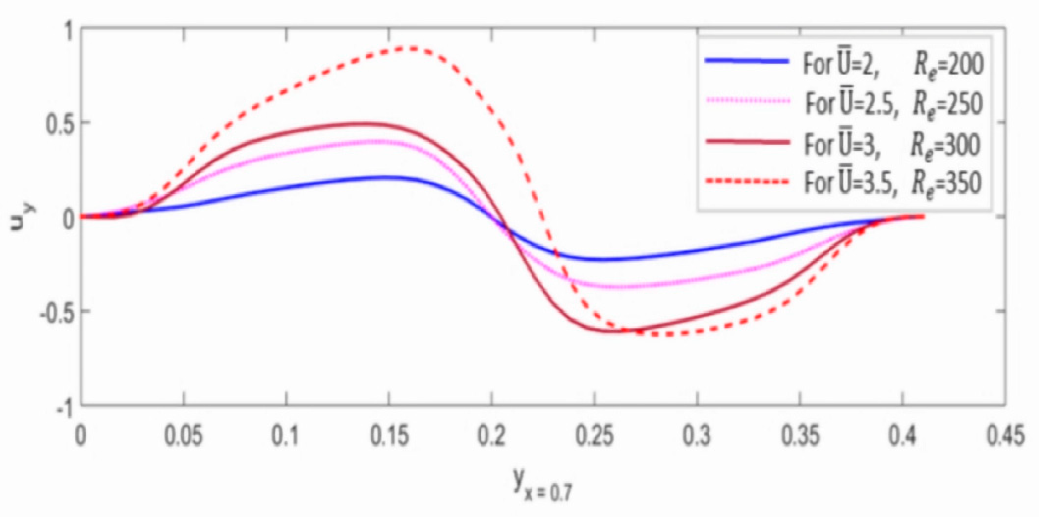
6.2. Analysis of Combined Effects of Linearly Increasing Reynolds Number and Mean Inflow Velocity

In the present study, the micro-structural characteristics of fluid flow are analyzed by increasing Reynolds number $R_e$ and mean inflow velocity $\overline{U}$ linearly. As it is known that flow velocity and Reynolds number are related directly, and the greater flow velocity results in a high Reynolds number. It is therefore observed from the obtained results that a uniform linear increase in Reynolds number $R_e$ and mean inflow velocity $\overline{U}$ show the significant combined effect on the micro-rotation velocity field $\mathsf{\omega }$, and this effect increases by increasing the values of both parameters. It is further noticed that although the micro-rotational effect increases with increasing values, the micro-rotation velocity profile maintains the same pattern at any particular location in the computational domain, as shown in Figure 6.

Furthermore, the combined effect of linearly increasing $R_e$ and $\overline{U}$ on the velocity field $u$ are also found very significant in a sense that horizontal and vertical velocity profiles show great variation by maintaining the same pattern on each increasing value of $R_e$ and $\overline{U}$ at any particular location in the computational domain, as displayed in Figure 7 and Figure 8, respectively. These results show similarity with those obtained by increasing micro-rotational viscosity ${\mu }_r$ [68] and can be interpreted as that fluid particles experience almost the same effect either by increasing Reynolds number $R_e$ and mean flow velocity $\overline{U}$ linearly or by increasing micro-rotational viscosity ${\mu }_r$. These results help us in understanding the behavior of fluid particles inside the computational domain at the micro-structural level in CFSI phenomena.

Finally, numerical values for the analysis of combined micro-structural effects of $R_e$ and $\overline{U}$ on flow velocity fields are given in

Table 4. Numerical values of $R_e$ and $\overline{U}$.

$\mathbf{Numerical} \mathbf{Values} \mathbf{of} \mathit{R}\mathit{e}$	$\mathbf{Numerical} \mathbf{Values} \mathbf{of} \overline{\mathbf{U}}$
200	2
250	2.5
300	3
350	3.5

.

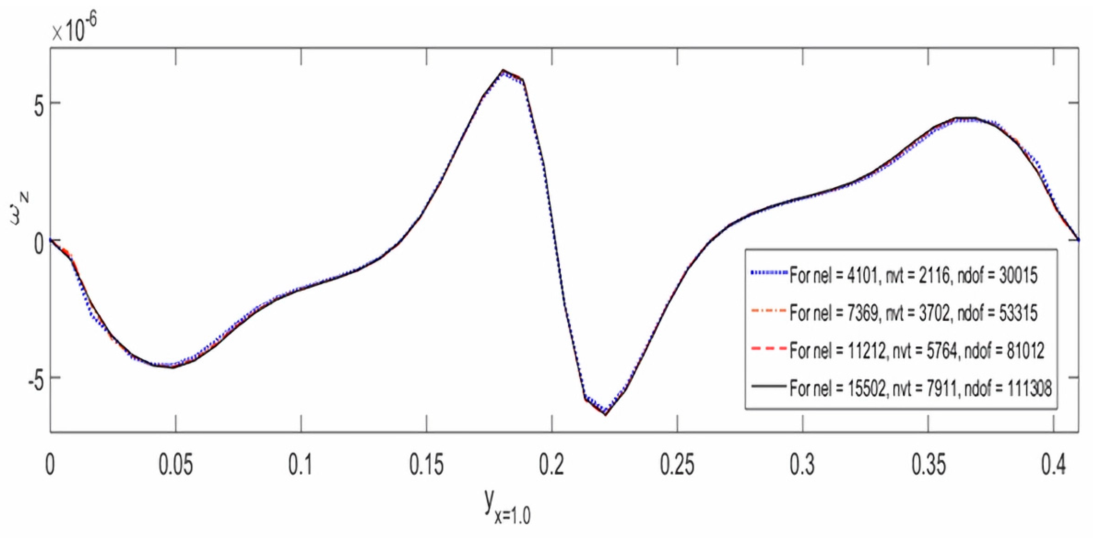
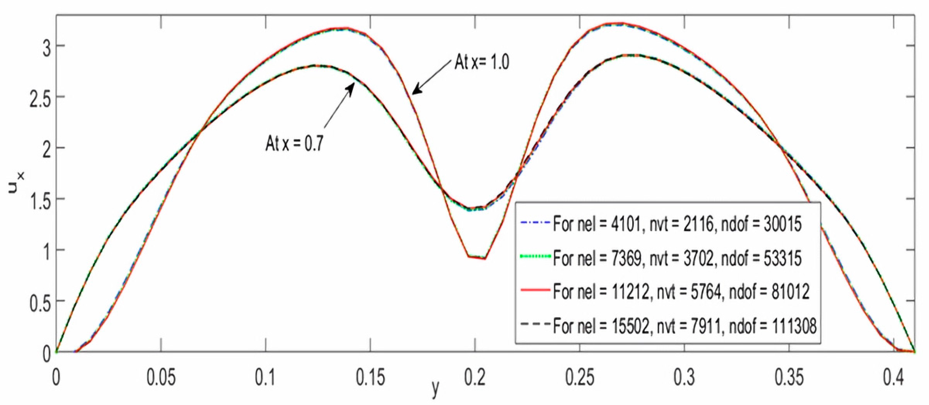
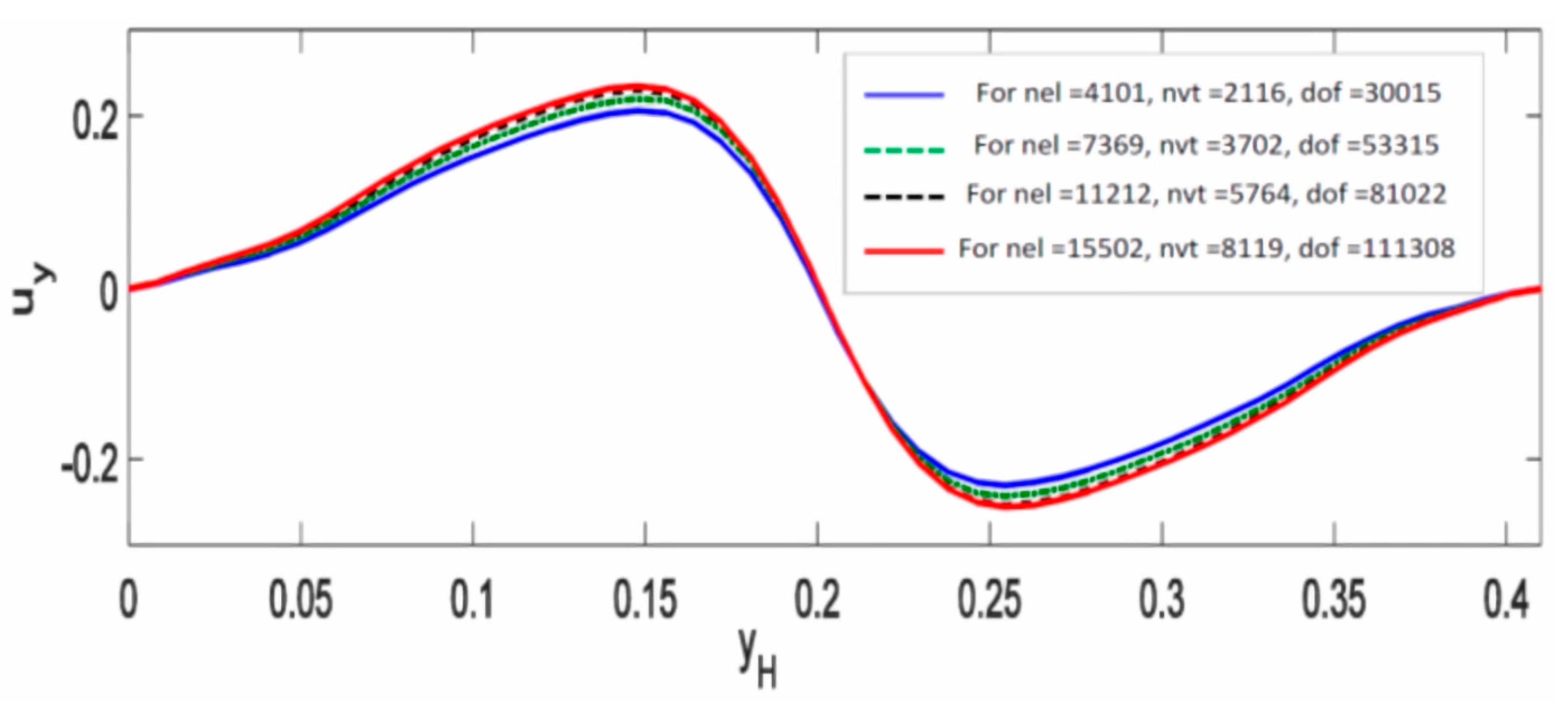
6.3. Mesh Independence Analysis

To check the desired accuracy of results obtained from computer simulations of the present study, it is very important to demonstrate the convergence of the obtained results using mesh independence analysis. Usually, mesh convergence ensures that the results obtained from the study are not affected by changing the size of the mesh. Following convergence, additional mesh refinement does not affect the results and is independent of the mesh. A mesh convergence study verifies that the proposed model has converged to a solution and provides a justification for mesh independence where additional refinement is unnecessary. To this aim, the mesh independence analysis is employed to verify the convergence of results obtained in this study, which are demonstrated for flow velocity fields in a non-classical framework, as shown in Figure 9, Figure 10 and Figure 11, respectively.

In the above mesh independence results, nel, nvt, and ndof represent the number of elements, the number of vertices, and the number of degrees of freedom, respectively. Further, it can be seen that all these mesh independence results nicely converge for different meshes taken into account, which validate and strengthen the results obtained during computer simulations for the present CFSI model in a non-classical framework.

Finally, a list of the number of elements, number of vertices, and number of degrees of freedom used for obtaining the flow velocity profiles against the mesh independence analysis are summarized in

Table 5. Data for the mesh independence flow velocity profiles.

Number of Elements (nel)	Number of Vertices (nvt)	Number of Degrees of Freedom (ndof)
4101	2116	30,015
7369	3702	53,315
11,212	5764	81,012
15,502	7911	111,308

.

7. Conclusions

In this paper, the combined effect of linearly increasing Reynolds number $R_e$ and mean inflow velocity $\overline{U}$ on flow velocity fields with mesh independence analysis has been studied by employing a monolithic Eulerian formulation to Cosserat fluid–structure interaction (CFSI) problems at a micro-structural level in a non-classical framework. The governing mathematical modeling of the CFSI problem has been derived using underlying laws of continuum mechanics. The results of the present study have been obtained by computing a prominent classical FSI benchmark test FLUSTRUK-FSI-3* with FreeFEM++ software. This benchmark test was validated by comparing the results with classical solutions present in the literature. The frequency $4.5 {\mathrm{s}}^{-1}$ and the amplitude $0.03$ of oscillations with a mesh of $2199$ vertices and a uniform time-step size of $0.005 \mathrm{s}$ validated the benchmark test in a non-classical framework. The results obtained indicated that a uniform linear increase in Reynolds number $Re$ and mean inflow velocity $\overline{U}$ produced a significant combined micro-structural effect on the micro-rotation velocity field $\mathsf{\omega }$, and a direct relation was found between the micro-rotational effect and both parameters. Moreover, this combined effect of increasing $R_e$ and $\overline{U}$ on the velocity field $u$ has also been observed as very significant in the sense that horizontal and vertical flow velocity profiles experienced great variation by maintaining the same pattern on each increasing value of $R_e$ and $\overline{U}$ at any particular location in the computational domain. Furthermore, the mesh independence analysis has been employed to verify the convergence of all results and demonstrated for flow velocity fields in a non-classical framework. The results converged nicely on employing the mesh independence analysis, which enhanced the desired accuracy of the obtained results and strengthened the governing modeling of the proposed CFSI problem. Further, the validation of the classical benchmark test made the results very significant and robust for the analysis of the micro-structural characteristics of fluid flow, especially using mesh independence analysis to ensure the desired accuracy of the obtained results. However, the implementation of algorithmic description requires enhanced computational resources to achieve the desired accuracy of results due to three additional micro-rotational degrees of freedom (dof), which makes the CFSI model very complex. Finally, the present study can be extended further for the analysis of the effects of micro-viscosity parameters on flow velocity fields for such coupling problems in a non-classical framework.

References

1. Morab, S.R.; Sharma, A. An Overview of Computational Fluid Structure Interaction: Methods and Applications. arXiv 2020, arXiv:2006.04068. [Google Scholar]
2. Faizollahzadeh Ardabili, S.; Najafi, B.; Shamshirband, S.; Minaei Bidgoli, B.; Deo, R.C.; Chau, K.W. Computational intelligence approach for modeling hydrogen production: A review. Eng. Appl. Comput. Fluid Mech. 2018, 12, 438–458. [Google Scholar] [CrossRef]
3. Akbarian, E.; Najafi, B.; Jafari, M.; Faizollahzadeh Ardabili, S.; Shamshirband, S.; Chau, K.W. Experimental and computational fluid dynamics-based numerical simulation of using natural gas in a dual-fueled diesel engine. Eng. Appl. Comput. Fluid Mech. 2018, 12, 517–534. [Google Scholar] [CrossRef]
4. Bazilevs, Y.; Takizawa, K. Advances in Computational Fluid-Structure Interaction and Flow Simulation; Birkhäuser: Basel, Switzerland, 2017. [Google Scholar]
5. Bodnár, T.; Galdi, G.P.; Nečasová, Š. (Eds.) Fluid-Structure Interaction and Biomedical Applications; Springer: Basel, Switzerland, 2014. [Google Scholar]
6. Bazilevs, Y.; Takizawa, K.; Tezduyar, T.E. Computational Fluid-Structure Interaction: Methods and Applications; John Wiley & Sons: Hoboken, NJ, USA, 2013. [Google Scholar]
7. Hou, G.; Wang, J.; Layton, A. Numerical methods for fluid-structure interaction—A review. Commun. Comput. Phys. 2012, 12, 337–377. [Google Scholar] [CrossRef]
8. Formaggia, L.; Quarteroni, A.; Veneziani, A. (Eds.) Cardiovascular Mathematics: Modeling and Simulation of the Circulatory System; Springer Science & Business Media: Berlin, Germany, 2010; Volume 1. [Google Scholar]
9. Ryzhakov, P.B.; Rossi, R.; Idelsohn, S.R.; Onate, E. A monolithic Lagrangian approach for fluid–structure interaction problems. Comput. Mech. 2010, 46, 883–899. [Google Scholar] [CrossRef]
10. Hron, J.; Turek, S. A monolithic FEM solver for an ALE formulation of fluid-structure interaction with configuration for numerical benchmarking. In Proceedings of the European Conference on Computational Fluid Dynamics, ECCOMAS CFD 2006, Egmond aan Zee, The Netherlands, 5–8 September 2006. [Google Scholar]
11. Hübner, B.; Walhorn, E.; Dinkler, D. A monolithic approach to fluid–structure interaction using space–time finite elements. Comput. Methods Appl. Mech. Eng. 2004, 193, 2087–2104. [Google Scholar] [CrossRef]
12. Michler, C.; Hulshoff, S.J.; Van Brummelen, E.H.; De Borst, R. A monolithic approach to fluid–structure interaction. Comput. Fluids 2004, 33, 839–848. [Google Scholar] [CrossRef]
13. Dunne, T. An Eulerian approach to fluid–structure interaction and goal-oriented mesh adaptation. Int. J. Numer. Methods Fluids 2006, 51, 1017–1039. [Google Scholar] [CrossRef]
14. Heil, M.; Hazel, A.L.; Boyle, J. Solvers for large-displacement fluid–structure interaction problems: Segregated versus monolithic approaches. Comput. Mech. 2008, 43, 91–101. [Google Scholar] [CrossRef]
15. Wang, Y.; Jimack, P.K.; Walkley, M.A.; Pironneau, O. An energy stable one-field monolithic arbitrary Lagrangian–Eulerian formulation for fluid–structure interaction. J. Fluids Struct. 2020, 98, 103117. [Google Scholar] [CrossRef]
16. Takahashi, T.; Batty, C. Monolith: A Monolithic Pressure-Viscosity-Contact Solver for Strong Two-Way Rigid-Rigid Rigid-Fluid Coupling; UWSpace: Waterloo, ON, Canada, 2020. [Google Scholar]
17. Zimmerman, A.G.; Kowalski, J. Monolithic Simulation of Ice-Shelf/Ocean Interaction with an Extended Enthalpy-Porosity Method for Convection-Coupled Phase-Change. In Proceedings of the EGU General Assembly 2019, Vienna, Austria, 7–12 April 2019. [Google Scholar]
18. Murea, C.M. Three-Dimensional Simulation of Fluid–Structure Interaction Problems Using Monolithic Semi-Implicit Algorithm. Fluids 2019, 4, 94. [Google Scholar] [CrossRef]
19. Schott, B.; Ager, C.; Wall, W.A. A monolithic approach to fluid-structure interaction based on a hybrid Eulerian-ALE fluid domain decomposition involving cut elements. Int. J. Numer. Methods Eng. 2019, 119, 208–237. [Google Scholar] [CrossRef]
20. Pironneau, O. An energy stable monolithic Eulerian fluid-structure numerical scheme. Chin. Ann. Math. Ser. B 2018, 39, 213–232. [Google Scholar] [CrossRef]
21. Sauer, R.A.; Luginsland, T. A monolithic fluid–structure interaction formulation for solid and liquid membranes including free-surface contact. Comput. Methods Appl. Mech. Eng. 2018, 341, 1–31. [Google Scholar] [CrossRef]
22. Langer, U.; Yang, H. Numerical simulation of fluid–structure interaction problems with hyperelastic models: A monolithic approach. Math. Comput. Simul. 2018, 145, 186–208. [Google Scholar] [CrossRef]
23. Hecht, F.; Pironneau, O. An energy stable monolithic Eulerian fluid-structure finite element method. Int. J. Numer. Methods Fluids 2017, 85, 430–446. [Google Scholar] [CrossRef]
24. Chiang, C.Y.; Pironneau, O.; Sheu, T.W.; Thiriet, M. Numerical study of a 3D Eulerian monolithic formulation for incompressible fluid-structures systems. Fluids 2017, 2, 34. [Google Scholar] [CrossRef]
25. Ata, K.; Sahin, M. A Monolithic Approach for the Incompressible Magneto-Hydrodynamics Equations. In Proceedings of the International Conference on Computational Methods for Coupled Problems in Science and Engineering (COUPLED), Rhodes Island, Greece, 12–14 June 2017. [Google Scholar]
26. Gatin, I.; Jasak, H.; Vukcevic, V. Monolithic coupling of rigid body motion and the pressure field in foam-extend. In Proceedings of the VII International Conference on Computational Methods in Marine Engineering, MARINE VII, Nantes, France, 15–17 May 2017; CIMNE: Barcelona, Spain, 2017; pp. 663–669. [Google Scholar]
27. Pironneau, O. Numerical study of a monolithic fluid–structure formulation. In Variational Analysis and Aerospace Engineering; Springer: Cham, Switzerland, 2016; pp. 401–420. [Google Scholar]
28. Langer, U.; Yang, H. Robust and efficient monolithic fluid-structure-interaction solvers. Int. J. Numer. Methods Eng. 2016, 108, 303–325. [Google Scholar] [CrossRef]
29. Langer, U.; Yang, H. Recent development of robust monolithic fluid-structure interaction solvers. Fluid-Structure Interaction. Modeling, Adaptive Discretization and Solvers. Radon Ser. Comput. Appl. Math. 2017, 20, 169–192. [Google Scholar]
30. Dunne, T.; Rannacher, R. Adaptive finite element approximation of fluid-structure interaction based on an Eulerian variational formulation. In Fluid-Structure Interaction; Springer: Berlin/Heidelberg, Germany, 2006; pp. 110–145. [Google Scholar]
31. Richter, T. A fully Eulerian formulation for fluid–structure-interaction problems. J. Comput. Phys. 2013, 233, 227–240. [Google Scholar] [CrossRef]
32. Wick, T. Fully Eulerian fluid–structure interaction for time-dependent problems. Comput. Methods Appl. Mech. Eng. 2013, 255, 14–26. [Google Scholar] [CrossRef]
33. Rannacher, R.; Richter, T. An adaptive finite element method for fluid-structure interaction problems based on a fully eulerian formulation. In Fluid Structure Interaction II; Springer: Berlin/Heidelberg, Germany, 2011; pp. 159–191. [Google Scholar]
34. Richter, T.; Wick, T. Finite elements for fluid–structure interaction in ALE and fully Eulerian coordinates. Comput. Methods Appl. Mech. Eng. 2010, 199, 2633–2642. [Google Scholar] [CrossRef]
35. Formaggia, L.; Gerbeau, J.F.; Nobile, F.; Quarteroni, A. On the coupling of 3D and 1D Navier–Stokes equations for flow problems in compliant vessels. Comput. Methods Appl. Mech. Eng. 2001, 191, 561–582. [Google Scholar] [CrossRef]
36. Nobile, F. Numerical Approximation of Fluid-Structure Interaction Problems with Application to Haemodynamics. Ph.D. Thesis, EPFL, Milan, Italy, 2001. [Google Scholar]
37. Le Tallec, P.; Mouro, J. Fluid structure interaction with large structural displacements. Comput. Methods Appl. Mech. Eng. 2001, 190, 3039–3067. [Google Scholar] [CrossRef]
38. Gerbeau, J.F.; Vidrascu, M. A quasi-Newton algorithm based on a reduced model for fluid-structure interaction problems in blood flows. ESAIM Math. Model. Numer. Anal. 2003, 37, 631–647. [Google Scholar] [CrossRef]
39. Fernández, M.A.; Moubachir, M. A Newton method using exact Jacobians for solving fluid–structure coupling. Comput. Struct. 2005, 83, 127–142. [Google Scholar] [CrossRef]
40. Dettmer, W.; Perić, D. A computational framework for fluid–structure interaction: Finite element formulation and applications. Comput. Methods Appl. Mech. Eng. 2006, 195, 5754–5779. [Google Scholar] [CrossRef]
41. Murea, C.M. Numerical simulation of a pulsatile flow through a flexible channel. ESAIM Math. Model. Numer. Anal. 2006, 40, 1101–1125. [Google Scholar] [CrossRef]
42. Mbaye, I.; Murea, C.M. Numerical procedure with analytic derivative for unsteady fluid–structure interaction. Commun. Numer. Methods Eng. 2008, 24, 1257–1275. [Google Scholar] [CrossRef]
43. Kuberry, P.; Lee, H. A decoupling algorithm for fluid-structure interaction problems based on optimization. Comput. Methods Appl. Mech. Eng. 2013, 267, 594–605. [Google Scholar] [CrossRef]
44. Schafer, G.S.; Sieber, R.; Teschauer, I. Coupled Fluid-Solid Problems: Examples and Reliable Numerical Simulation. In Proceedings of the Trend in Computational Structural Mechanics; International Center for Numerical Methods in Engineering CIMNE: Barcelona, Spain, 2001. [Google Scholar]
45. Piperno, S.; Farhat, C.; Larrouturou, B. Partitioned procedures for the transient solution of coupled aroelastic problems Part I: Model problem, theory and two-dimensional application. Comput. Methods Appl. Mech. Eng. 1995, 124, 79–112. [Google Scholar] [CrossRef]
46. Piperno, S. Explicit/implicit fluid/structure staggered procedures with a structural predictor and fluid subcycling for 2D inviscid aeroelastic simulations. Int. J. Numer. Methods Fluids 1997, 25, 1207–1226. [Google Scholar] [CrossRef]
47. Mok, D.P.; Wall, W.A.; Ramm, E. Accelerated iterative substructuring schemes for instationary fluid-structure interaction. Comput. Fluid Solid Mech. 2001, 2, 1325–1328. [Google Scholar]
48. Richter, T. Numerical Methods for Fluid-Structure Interaction Problems; Institute for Applied Mathematics, University of Heidelberg: Berlin/Heidelberg, Germany, 2010. [Google Scholar]
49. Donea, J. Arbitrary Lagrangian-Eulerian finite element analysis. Comput. Methods Transient Anal. 1983, 474–516. [Google Scholar]
50. Quarteroni, A.; Formaggia, L. Mathematical modelling and numerical simulation of the cardiovascular system. Handb. Numer. Anal. 2004, 12, 3–127. [Google Scholar]
51. Nobile, F.; Vergara, C. An effective fluid-structure interaction formulation for vascular dynamics by generalized Robin conditions. SIAM J. Sci. Comput. 2008, 30, 731–763. [Google Scholar] [CrossRef]
52. Formaggia, L.; Quarteroni, A.; Veneziani, A. Cardiovascular Mathematics, Volume 1 of MS&Modeling, A; Simulation and Applications; Springer Science & Business Media: Berlin, Germany, 2009. [Google Scholar]
53. Le Tallec, P.; Hauret, P. Energy conservation in fluid structure interactions. Numer. Methods Sci. Comput. Var. Probl. Appl. 2003, 94–107. [Google Scholar]
54. Basting, S.; Quaini, A.; Čanić, S.; Glowinski, R. Extended ALE method for fluid–structure interaction problems with large structural displacements. J. Comput. Phys. 2017, 331, 312–336. [Google Scholar] [CrossRef]
55. Liu, J. A second-order changing-connectivity ALE scheme and its application to FSI with large convection of fluids and near contact of structures. J. Comput. Phys. 2016, 304, 380–423. [Google Scholar] [CrossRef]
56. Peskin, C.S. The immersed boundary method. Acta Numer. 2002, 11, 479–517. [Google Scholar] [CrossRef]
57. Coupez, T.; Silva, L.; Hachem, E. Implicit boundary and adaptive anisotropic meshing. In New Challenges in Grid Generation and Adaptivity for Scientific Computing; Springer: Cham, Switzerland, 2015; pp. 1–18. [Google Scholar]
58. Robinson-Mosher, A.; Shinar, T.; Gretarsson, J.; Su, J.; Fedkiw, R. Two-way coupling of fluids to rigid and deformable solids and shells. ACM Trans. Graph. TOG 2008, 27, 1–9. [Google Scholar] [CrossRef]
59. Boffi, D.; Cavallini, N.; Gastaldi, L. The finite element immersed boundary method with distributed Lagrange multiplier. SIAM J. Numer. Anal. 2015, 53, 2584–2604. [Google Scholar] [CrossRef]
60. Wang, Y.; Jimack, P.K.; Walkley, M.A. A one-field monolithic fictitious domain method for fluid–structure interactions. Comput. Methods Appl. Mech. Eng. 2017, 317, 1146–1168. [Google Scholar] [CrossRef]
61. Afra, B.; Delouei, A.A.; Mostafavi, M.; Tarokh, A. Fluid-structure interaction for the flexible filament’s propulsion hanging in the free stream. J. Mol. Liq. 2021, 323, 114941. [Google Scholar] [CrossRef]
62. Hajano, N.H.; Khan, M.S.; Liu, L. Increasing Micro-Rotational Viscosity Results in Large Micro-Rotations: A Study Based on Monolithic Eulerian Cosserat Fluid–Structure Interaction Formulation. Mathematics 2022, 10, 4188. [Google Scholar] [CrossRef]
63. Cosserat, E.; Cosserat, F. Theorie des Corps Déformables; A. Hermann et Fils: Paris, France, 1909. [Google Scholar]
64. Eringen, A.C. Theory of micropolar fluids. J. Math. Mech. 1966, 16, 1–18. [Google Scholar] [CrossRef]
65. Eringen, A.C. Simple microfluids. Int. J. Eng. Sci. 1964, 2, 205–217. [Google Scholar] [CrossRef]
66. Condiff, D.W.; Dahler, J.S. Fluid mechanical aspects of antisymmetric stress. Phys. Fluids 1964, 7, 842–854. [Google Scholar] [CrossRef]
67. Bazdar, H.; Toghraie, D.; Pourfattah, F.; Akbari, O.A.; Nguyen, H.M.; Asadi, A. Numerical investigation of turbulent flow and heat transfer of nanofluid inside a wavy microchannel with different wavelengths. J. Therm. Anal. Calorim. 2020, 139, 2365–2380. [Google Scholar] [CrossRef]
68. Arasteh, H.; Mashayekhi, R.; Goodarzi, M.; Motaharpour, S.H.; Dahari, M.; Toghraie, D. Heat and fluid flow analysis of metal foam embedded in a double-layered sinusoidal heat sink under local thermal non-equilibrium condition using nanofluid. J. Therm. Anal. Calorim. 2019, 138, 1461–1476. [Google Scholar] [CrossRef]
69. Oveissi, S.; Toghraie, D.; Eftekhari, S.A. Longitudinal vibration and stability analysis of carbon nanotubes conveying viscous fluid. Phys. E Low-Dimens. Syst. Nanostructures 2016, 83, 275–283. [Google Scholar] [CrossRef]
70. Lukaszewicz, G. Micropolar Fluids: Theory and Applications; Springer Science & Business Media: Berlin, Germany, 1999. [Google Scholar]
71. Hecht, F. New development in FreeFem++. J. Numer. Math. 2012, 20, 251–266. [Google Scholar] [CrossRef]
72. Kim, C.; Jung, M.; Yamada, T.; Nishiwaki, S.; Yoo, J. Freefem++ code for reaction-diffusion equation–based topology optimization: For high-resolution boundary representation using adaptive mesh refinement. Struct. Multidiscip. Optim. 2020, 62, 439–455. [Google Scholar] [CrossRef]
73. Dapogny, C.; Frey, P.; Omnès, F.; Privat, Y. Geometrical shape optimization in fluid mechanics using FreeFem++. Struct. Multidiscip. Optim. 2018, 58, 2761–2788. [Google Scholar] [CrossRef]
74. Krivovichev, G.V. A computational approach to the modeling of the glaciation of sea offshore gas pipeline. Int. J. Heat Mass Transf. 2017, 115, 1132–1148. [Google Scholar] [CrossRef]
75. Belytschko, T.; Liu, W.K.; Moran, B.; Elkhodary, K. Nonlinear Finite Elements for Continua and Structures; John Wiley & Sons: Hoboken, NJ, USA, 2014. [Google Scholar]
76. Batra, R.C. Elements of Continuum Mechanics; AIAA: Reston, VA, USA, 2006. [Google Scholar]
77. Bath, K.J. Finite Element Procedures; Prentice-Hall: Englewood Cliffs, NJ, USA, 1996. [Google Scholar]
78. Marsden, J.; Hughes, T.J.R. Mathematical Foundations of Elasticity; Dover Publications: New York, NY, USA, 1993. [Google Scholar]
79. Ciarlet, P.G. Mathematical Elasticity: Volume 1: Three-Dimensional Elasticity; North Holland Publishing Company: Amsterdam, The Netherlands, 1988. [Google Scholar]
80. Schafer, M.; Turek, S. Benchmark computations of laminar flow around a cylinder. Notes Numer. Fluid Mech. 1996, 52, 547–566. [Google Scholar]
81. Turek, S.; Hron, J. Proposal for numerical benchmarking of fluid-structure interaction between an elastic object and laminar incompressible flow. In Fluid-Structure Interaction; Springer: Berlin, Heidelberg, 2006; pp. 371–385. [Google Scholar]
82. American Society of Mechanical Engineers. Standard for Verification and Validation in Computational Fluid Dynamics and Heat Transfer: An American National Standard; American Society of Mechanical Engineers: New York, NY, USA, 2009. [Google Scholar]
Figure 1. Collapse of Tacoma Narrows Bridge (1940) (Source: Wikipedia).
Mathematics 11 02074 g001
Figure 2. An overview of monolithic and partitioned approaches.
Mathematics 11 02074 g002
Figure 3. Cosserat fluid–structure interaction domain and notations.
Mathematics 11 02074 g003
Figure 4. Horizontal displacement of flagella end tip against time.
Mathematics 11 02074 g004
Figure 5. Vertical displacement of flagella end tip against time.
Mathematics 11 02074 g005
Figure 6. The micro-rotation velocity profile against increasing R e and U ¯ at horizontal location x = 0.7 .
Mathematics 11 02074 g006
Figure 7. The horizontal velocity profile against increasing R e and U ¯ at horizontal location x = 0.7 .
Mathematics 11 02074 g007
Figure 8. The vertical velocity profile against increasing R e and U ¯ at horizontal location x = 0.7 .
Mathematics 11 02074 g008
Figure 9. Micro-rotation velocity profile against mesh independence.
Mathematics 11 02074 g009
Figure 10. Horizontal velocity profile against mesh independence.
Mathematics 11 02074 g010
Figure 11. Vertical velocity profile against mesh independence.
Mathematics 11 02074 g011