Article

Complex Color Space Segmentation to Classify Objects in Urban Environments

by
Juan-Jose Cardenas-Cornejo
,
Mario-Alberto Ibarra-Manzano
,
Daniel-Alberto Razo-Medina
and
Dora-Luz Almanza-Ojeda
*,†
Electronics Engineering Department, DICIS, University of Guanajuato, Carr. Salamanca-Valle de Santiago KM. 3.5 + 1.8 Km., Salamanca 36885, Mexico
*
Author to whom correspondence should be addressed.
These authors contributed equally to this work.
Mathematics 2022, 10(20), 3752; https://doi.org/10.3390/math10203752
Submission received: 8 September 2022 / Revised: 4 October 2022 / Accepted: 6 October 2022 / Published: 12 October 2022
(This article belongs to the Special Issue Applied and Computational Mathematics for Digital Environments)

Abstract

:
Color image segmentation divides the image into areas that represent different objects and focus points. One of the biggest problems in color image segmentation is the lack of homogeneity in the color of real urban images, which generates areas of over-segmentation when traditional color segmentation techniques are used. This article describes an approach to detecting and classifying objects in urban environments based on a new chromatic segmentation to locate focus points. Based on components a and b on the CIELab space, we define a chromatic map on the complex space to determine the highest threshold values by comparing neighboring blocks and thus divide various areas of the image automatically. Even though thresholds can result in broad segmentation areas, they suffice to locate centroids of patches on the color image that are then classified using a convolutional neural network (CNN). Thus, this broadly segmented image helps to crop only outlying areas instead of classifying the entire image. The CNN is trained to use six classes based on the patches drawn from the database of reference images from urban environments. Experimental results show a high score for classification accuracy that confirms the contribution of this segmentation approach.

1. Introduction

Autonomous systems need to recognize objects and their position in the real world to interact. Ideally, autonomous systems label objects and regions on an image to understand the environment [1]. Commonly used strategies in smart systems are based on image segmentation and automatic-learning techniques. Image segmentation is a key task in computer vision involving the analysis of standard features, such as texture and color, among others, on the image. However, most models and techniques used in image segmentation are unique, that is to say, only used for a specific purpose, and their performance only differs depending on the color space involved [2]. Therefore, choosing a suitable space to represent color is essential during the segmentation process.
CIELab, HSI [3] or HSV [4] are the most common color spaces used to segment images. Others, such as M u n s e l or Y I Q spaces [5], are used for several purposes and need specific methodologies to work. The CIELab color space mimics how humans perceive color; it is useful to modify brightness and color values on an image independently [6]. Most processing techniques based on the CIELab color space analyze each plane individually. According to the CIELab theory, chromatic components a and b are orthogonal axes on a 2D plane. Thus, the representation of 2D space on CIELab can be transformed into complex space directly, enabling the possibility of using complex numbers to facilitate algebraic calculations of image data.
A complex number is a pair of real numbers a and b ordered as ( a , b ) , and expressed as a + b i whereby i is the imaginary unit defined as i 2 = 1 . The symbol z can represent any complex number and is a complex variable subject to operational definitions, such as an addition and a multiplication [7]. Each complex number corresponds to a single point on the complex plane.
On the other hand, automatic learning only extracts data from the most representative objects and regions to classify as segmented images. A good selection of segmentation techniques considers the relevant context, hardware resources, the number of classes, and the size of the dataset [8]. For instance, in classifying the object in the self-driving, hardware resources and the number of classes play a key role because the size of the training data and validation labels could restrict decision-making. A self-driving car that uses deep learning needs to consider hardware resources to process the dataset [9]. A convolutional neural network (CNN) is related to the number of convolutional layers, the kind of layer grouping, the activation function used, the number of fully connected layers, and the size of the image to be processed as well as the techniques used to prevent over adjustment. Even though the training phase of a CNN is computationally costly, these models can reach high classification accuracy levels, making them popular.
This study proposes using a color image segmentation algorithm based on a chromatic map defined on a space using complex numbers to analyze the best color distribution. Complex algebra is used spatially to obtain final representative thresholds to segment the image. The segmented images represent similar chromatic values on components a and b of the CIELab space and the image’s most relevant areas. Patches from representative areas are extracted based on both aspects. A convolutional neural network (CNN) classifies the extracted patches to label them on the color image. This study’s contribution is to propose a new representation of chromatic components based on complex numbers defined as a chromatic map. The map can facilitate localizing the most representative areas across the image using fundamental algebra for complex numbers. This segmentation method renders broadly segmented images; however, instead of refining the segmented areas and labeling them, several patches from the color images are extracted using the location of the segmented area as the input for a CNN classifier. Thus, this segmentation strategy is a phase prior to the classifier that looks for similar chromatic patterns that represent the essential content of the image. This approach to segmentation and classification has been tested using urban-context images, and the results include data about the reliability of each predicted image class.

2. Related Works

Labeling segmented areas require high computational resources to recognize objects during the human−machine interaction. Image segmentation is often based on the graphs theory and grouping algorithms. In [10], the authors propose a general scheme of segmentation of scenes based on the spectral grouping algorithm for normalized cuts, fusing geometric and color information on a working frame with no parameters. The study in [11] presents a segmentation scheme to combine color and depth information. Under this scheme, segmentation happens in 3 steps. The study by Karimpoulit [12] identifies the types of rocks using images of rocky settings. Segmentation has been extended to video; for instance, the authors of [13] have developed a method to combine the appearance of an object with the temporal consistency between frames. Using the features of a normalized-color histogram and CNN features, the GrabCut algorithm is applied to different frame boundaries to segment the object in the background. When detecting objects in motion, the background is obtained using videos taken from a static camera. The study presented in [14] suggests the option of a detection and segmentation method based on consecutive stereo images that process dynamic objects found in an urban environment. This is a pixel-by-pixel approach applied to the KITTI dataset [15], and the frame boundaries are generated bearing in mind color and difference data for each moving object.
Unlike object-detection strategies, object recognition focuses on the objectives of the image and provides a specific class for each one [16]. As the objective is better adjusted to the frame boundary, the classification results become more reliable without a background. The fast development of smart vehicles makes object detection and recognition essential in self-driving [1]. In addition, road sign detection provides key information for safe navigation. Often, road detection is based on standard low-profile features used to process the image and isolate the borders. In [17], a real-time two-stage YOLOv2-based road-sign detection system is used. In the first stage, the YOLOv2 detection frame is modified to adapt it to the road-sign detection task and predicts boundary frames, class, and reliability of road signage. In the second stage, an invariant light road-sign transformation network (RM-Net) reclassifies the samples with low accuracy to increase accuracy.
The CNN architectures used for segmentation purposes are usually of three kinds, fully convolutional networks (FCN) [18], coder-decoder networks [19] and “atrous-convolutional” networks [20]. The authors in [21] introduce the Mask R-CNN method, an extension of the Faster R-CNN method [22] to segment images instead of just detecting boundary frames. There are also some approaches whereby Deep Neural Networks are modified, for instance, semantic-aware segmentation [23] to use semantic segmentation and instance segmentation. Recent strategies propose general DWT and IDWT layers to various wavelets and design wavelet integrated CNNs (WaveCNets) for image classification using ImageNet and ImageNet-C, achieving an accuracy of 78.51 %  [24]. Moreover, a new architecture (VOLO) implements a novel outlook attention operation that dynamically conducts the local feature aggregation mechanism in a sliding window across the input image. This approach uses transformers and CNNs to complement their model and achieves 87.1 % using ImageNet-1k [25]. Another natural color image approach is described in [26]. In this approach, the image is split into patches that feed the embedding module to expand the feature dimensions used for image classification [26]. This method achieves 83.9 % in the Top-1 accuracy rate.
The main aims of this study are: (1) to develop an automatic strategy to obtain areas on a natural, outdoor image transforming components a and b of the CIELab image as a complex space to represent image tonality, saturation, and contrast; (2) to build a chromatic map that concentrates the distribution of the tone density of pixels from the image using algebra for complex numbers; (3) to provide a strategy that includes sky and road categories, which are usually considered in semantic-based methods but not in object-classifier methods.

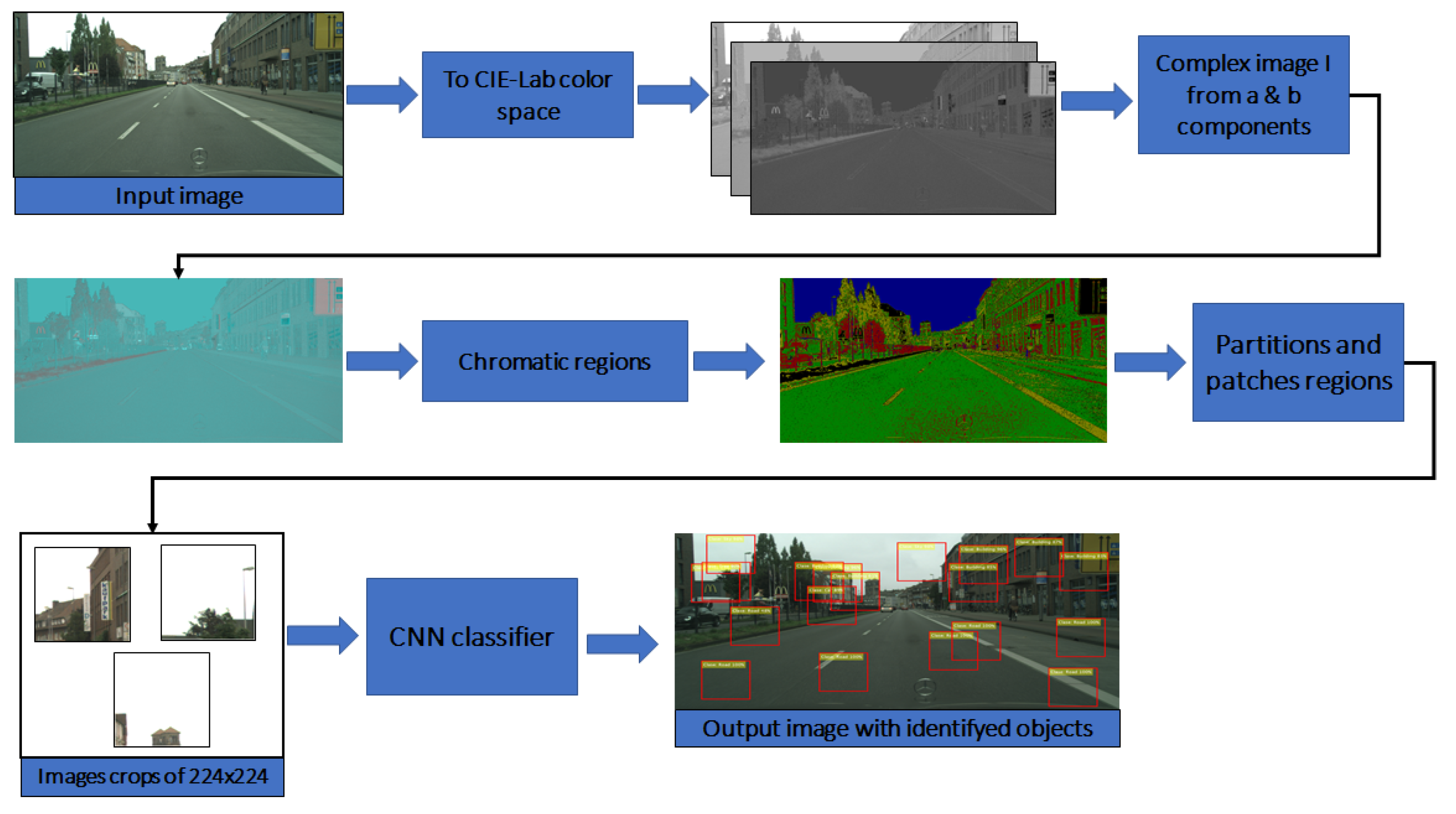
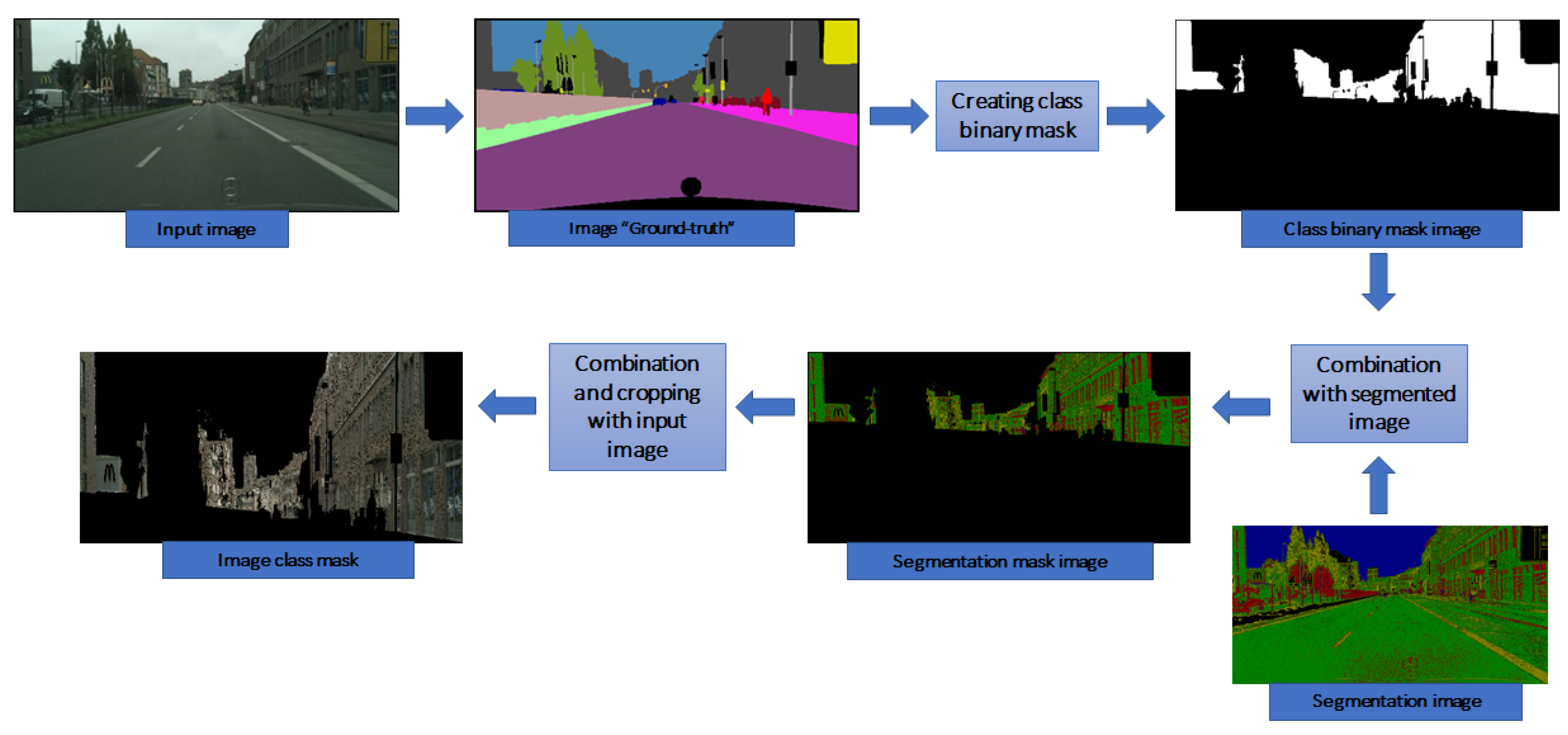
3. Image Segmentation Approach

Figure 1 shows an overview of the proposed method to segment images and identify objects. First, input color images are transformed to the CIELab space. Next, chromatic planes a and b on the CIELab space are used as real and imaginary elements to form complex image I. The representative chromatic values of image I are calculated using the complex image to build a chromatic map. The number of thresholds per image depends on the colors of the image. The segmented areas represent those from images with similar chromatic values without a classification label. The next step consists of extracting several patches from the color image from each segmented area to build a database of images in six categories. A CNN uses the database to train, validate and test the identification of the object on the image. Note that color image patches are the input to the CNN model instead of the segmented areas. The implementation details of the method are shown in the following subsection.

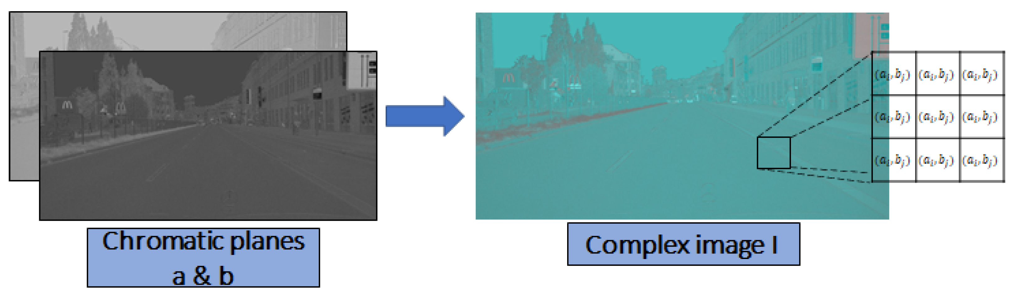
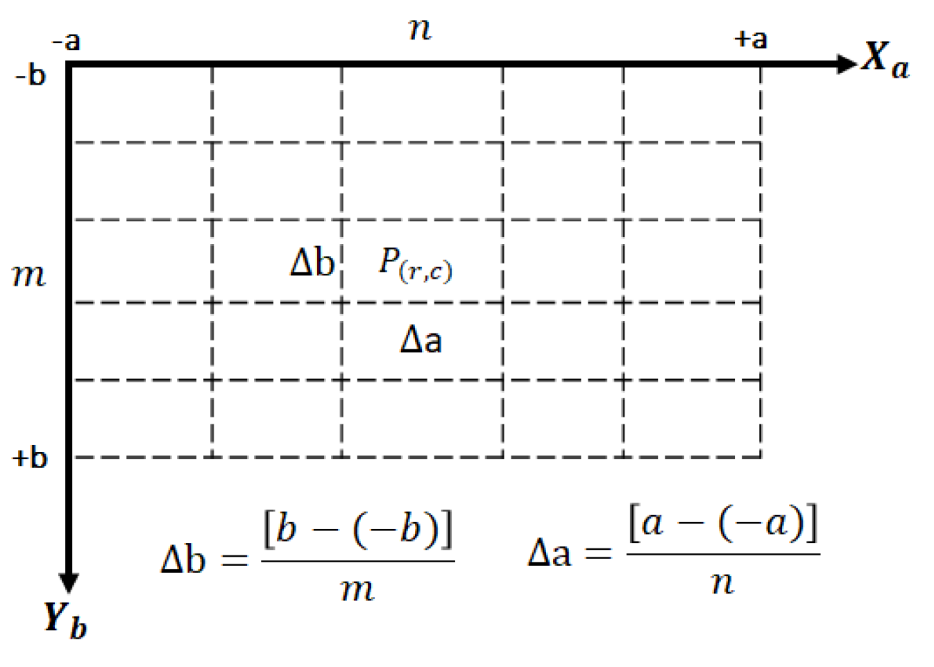
3.1. Image in the Complex Space
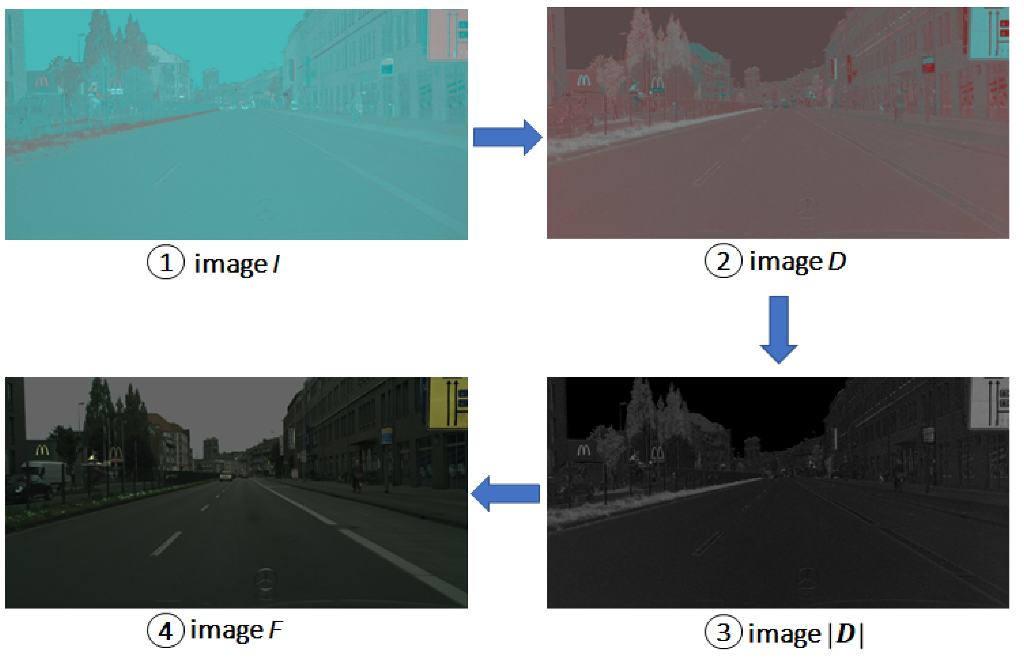
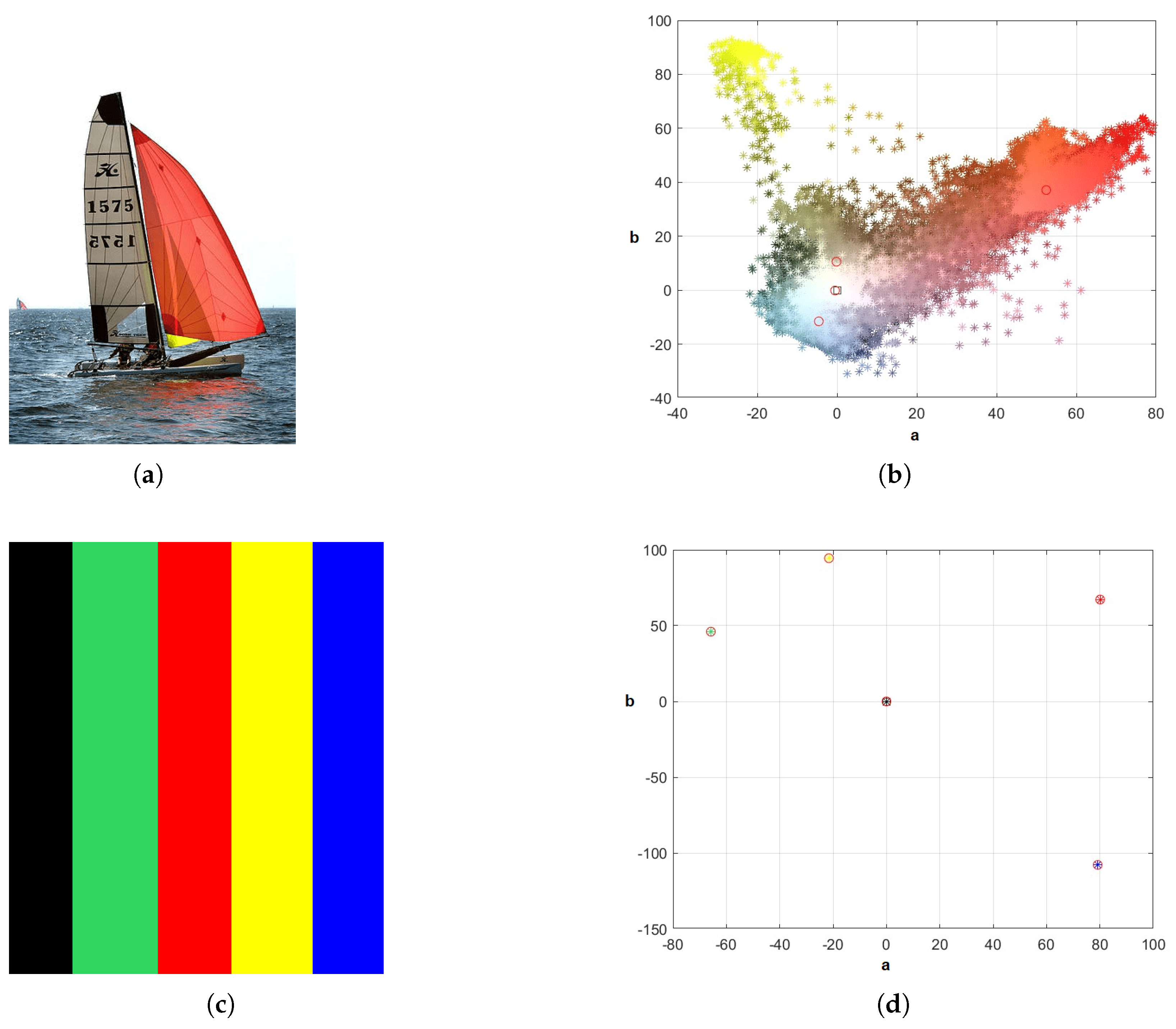
As said earlier, planes a and b on the CIELab space known as i m A and i m B , are combined to generate complex image I. Figure 2 shows chromatic planes i m A and i m B to form complex image I for a specific color image. Each pixel on image I is a complex number z = a + i b , processed using algebra for complex numbers. In this case, basic operations such as division, modulus, and argument have been used [27], but the division is the main operation used. Each pixel I is divided by a reference point P ( r , c ) ; the resulting image is known as the division image and is referred to as D. Image D shows values such as the threshold ones indicated by reference point P ( r , c ) within boundary ϵ . Thus, the same values as the unit or those close to it point to similar areas as those of the threshold value P ( r , c ) . Equation (1) defines division image D, which is the resulting complex image I size u × v divided by reference point P ( r , c ) . Values close to the unity in D represent similar pixels as those of P ( r , c ) . Therefore, image D shows the relevance of point P ( r , c ) on the color image. However, as D is in the complex space, searching for values close to 1 cannot be direct. Using module D, the image of module D can generate positive real values.
D [ u × v ] = I [ u × v ] P ( r , c )
In Equation (2), unitary values in D (around an ϵ value) are chosen to obtain the thresholded image F and to highlight areas with a color such as P ( r , c ) . Figure 3 represents the Division image D and the corresponding module D . D shows in white color the areas whose values are similar to P ( r , c ) .
F [ u × v ] = 1 if 1 ϵ D [ u × v ] 1 + ϵ 0 otherwise
To obtain a final segmented image F, first, representative P ( r , c ) thresholds must be found. Each threshold requires the division process. A chromatic map AB makes it possible to obtain several thresholds for the image automatically.

3.2. Chromatic Map

Chromatic map AB can be defined in the context of a bidimensional histogram. Chromatic components a and b on the CIELab space make up the horizontal X a and vertical Y b axis on the map AB . This can be illustrated as shown in Figure 4a,c for a real and an artificial image, respectively.
Figure 4d shows five representative points on the chromatic map AB , one for each area of the artificial image shown in Figure 4c. These points separate the chromatic components of the image. In the case of images such as those in Figure 4a, chromatic values are calculated by seeking the most representative values, that is to say, the highest density of points. Therefore, chromatic map AB is divided into k-areas, resulting from division m and n on the Y b and X a axes, respectively. Thus, the map is divided into k = m × n areas based on the combinations of m and n within the set of values 4 , 8 , 16 , 32 . These values reduce the complexity of the power and make the methodology suitable for hardware implementation. For instance, blocks k = 128 when dividing the map by m = 8 and n = 16 .
In Equation (3), n p x is a percentage based on the total number of pixels on the image, which is used to label blocks as representative. Each block has a chromatic range Δ a and Δ b defined by Equations (4) and (5). Figure 5 shows the division in k−blocks on a chromatic map, whose axes take the chromatic values from planes a and b on the CIELab space used to build complex image I.
n p x = u × v · 1 m a x m , n
Δ a = m a x ( X a ) m i n ( X a ) m
Δ b = m a x ( Y b ) m i n ( Y b ) n

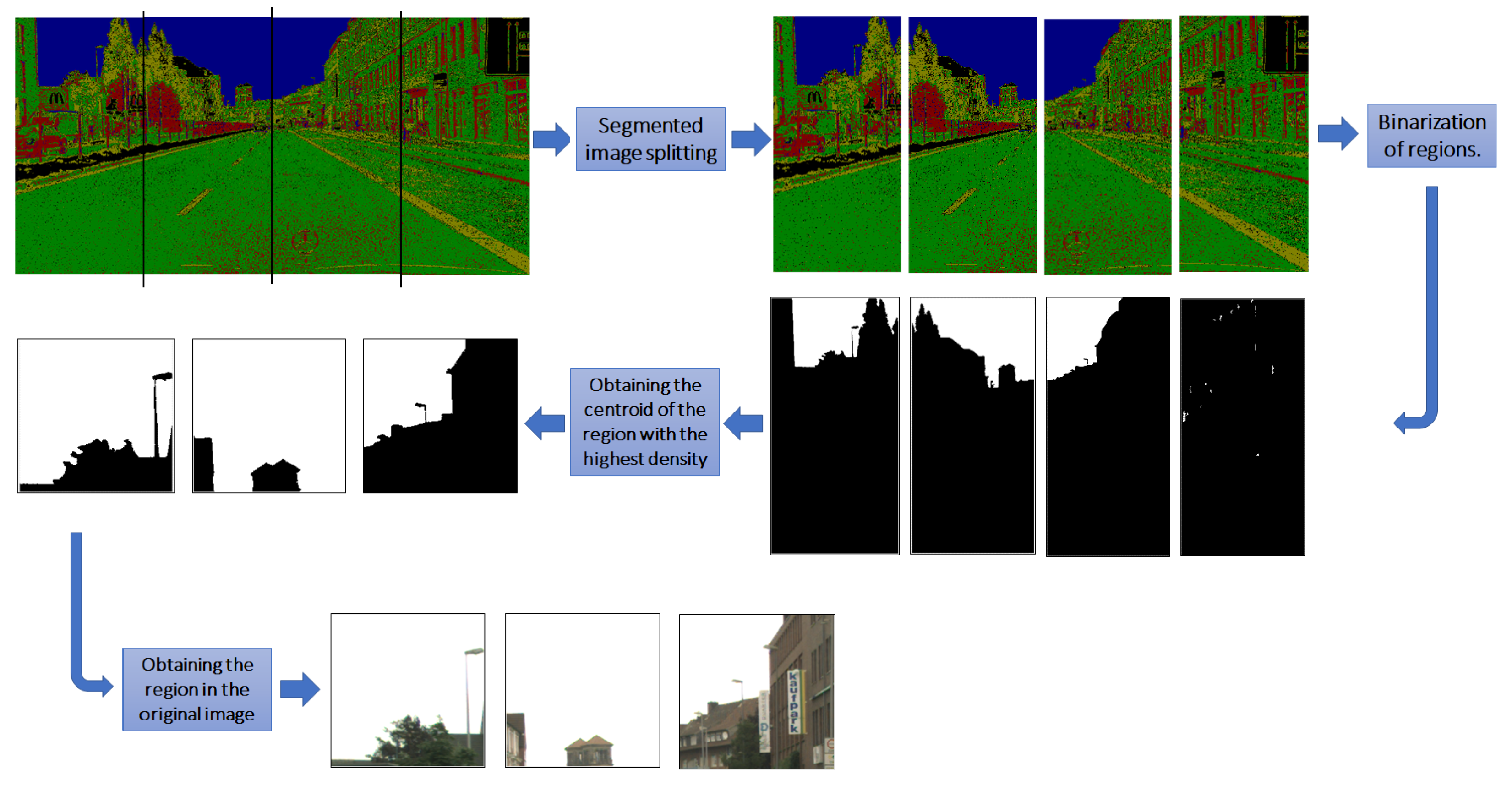
3.3. Segmentation Approach

This study uses complex numbers to segment the complex image I. As shown in the previous subsection, the chromatic map AB represents the pixel density distribution along k-blocks on the complex image. In each block ( i , j ) on the chromatic map AB , density M μ is calculated by counting the number of pixels M p and averaging the intensity of each pixel on I, as shown in Equation (6).
M μ i , j = p = 1 M p I i , j p M p if M p > 0 0 in   another   case
Equation (7) calculates indexes i n d M p , showing blocks with a number of pixels greater than n p x . In Equation (8), a second criterion is applied to obtain the final vector index i n d M μ , which stores the indexes for blocks on M μ , which also agrees with i n d M p . The number of thresholds n t h is used in the segmentation process and is obtained from the cardinality of vector i n d M μ (see Equation (9)).
i n d M p = M p n p x
i n d M μ = M μ i n d M p
n t h = c a r d i n d M μ
Vector V μ is calculated using M μ and i n d M μ , as shown in Equation (10). V μ is the vector for average values used as thresholds in the segmentation process, which are still represented using complex numbers. The correlation matrix M c o r r is obtained by dividing each threshold value by all the other values, as shown in Equation (11). Equation (12) represents the areas for average values bound by a circle | z z 0 | = R . In this case, areas are defined as being within a unitary circle centered on each threshold value on the matrix  M c o r r .
V μ = M μ i n d M μ
M c o r r i , j = V μ i V μ j i , j = { 1 , , n t h }
M r μ = 1 M c o r r = 1 V μ 1 V μ 1 1 V μ 1 V μ 2 1 V μ 1 Z μ k 1 V μ 2 V μ 1 1 V μ 2 V μ 2 1 V μ 2 V μ k 1 V μ k V μ 1 1 V μ k V μ 2 1 V μ k V μ k
The matrix values M r μ are used to analyze the middle values. Beyond diagonal values, minimization was conducted on matrix M r μ . Minimum values obtained are then divided by two to ensure there is no overlap between areas centered around average values; this is expressed by V r μ in Equation (13). n t h values are stored in V r μ , which contains the thresholds to conduct color segmentation. Algorithm 1 explains the implementation of the multi-threshold segmentation process on a color image.
V r μ = min M r μ i , j 2 i j
Algorithm 1 Segmentation method
Input:
Input image im, number of blocks m , n in the chromatic map
Output:
Segmented image imSeg
1:
n p x s i z e ( im ) m a x ( m , n )
2:
[ i m L , i m A , i m B ] t o _ c i e l a b ( im )
3:
I i m A + i i m B      % c o m p l e x i m a g e
4:
for  i = 1  to m do
5:
    for  j = 1  to n do
6:
         M p c a r d ( b l o c k i , j )
7:
        if  M p > 0  then
8:
            M μ m e a n ( b l o c k i , j )
9:
        end if
10:
  end for
11:
end for
12:
i n d M p ( M p n p x )
13:
i n d M μ M μ ( i n d M p ) ;
14:
[ V μ , n t h ] [ M μ i n d M μ , c a r d ( i n d M μ ) ]
15:
for  i , j = 1  to  n t h  do
16:
     M c o r r ( i , j ) V μ ( i ) V μ ( j )
17:
end for
18:
M r μ abs 1 abs M c o r r
19:
V r μ min M r μ ( i , j ) 2 for i j
20:
for  k = 1  to  n t h  do
21:
    if  V r μ k 0  then
22:
         D I V r μ ( k )
23:
    else
24:
         D abs I
25:
    end if
26:
     F abs 1 abs D
27:
     S ( : , : , k ) k · F < V r μ ( k )
28:
     i m g S e g S ( : , : , k ) k k
29:
end for

4. Results

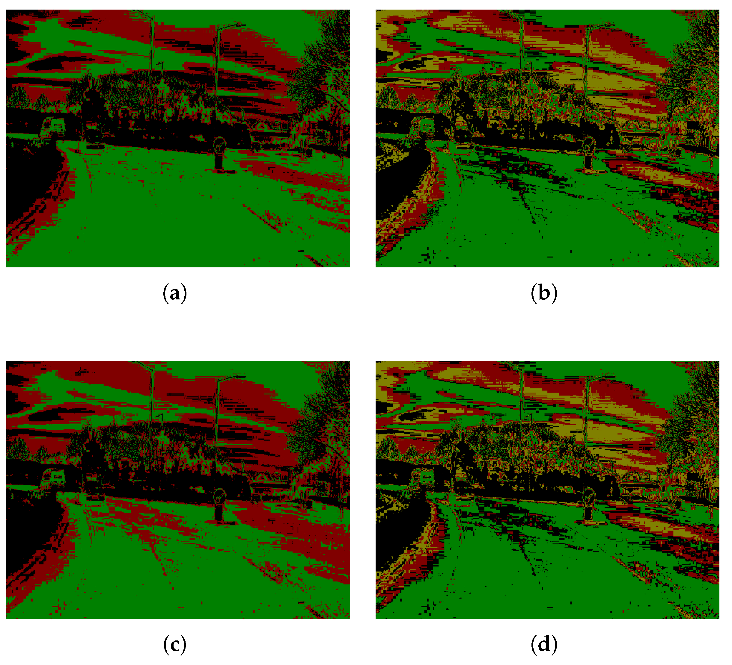
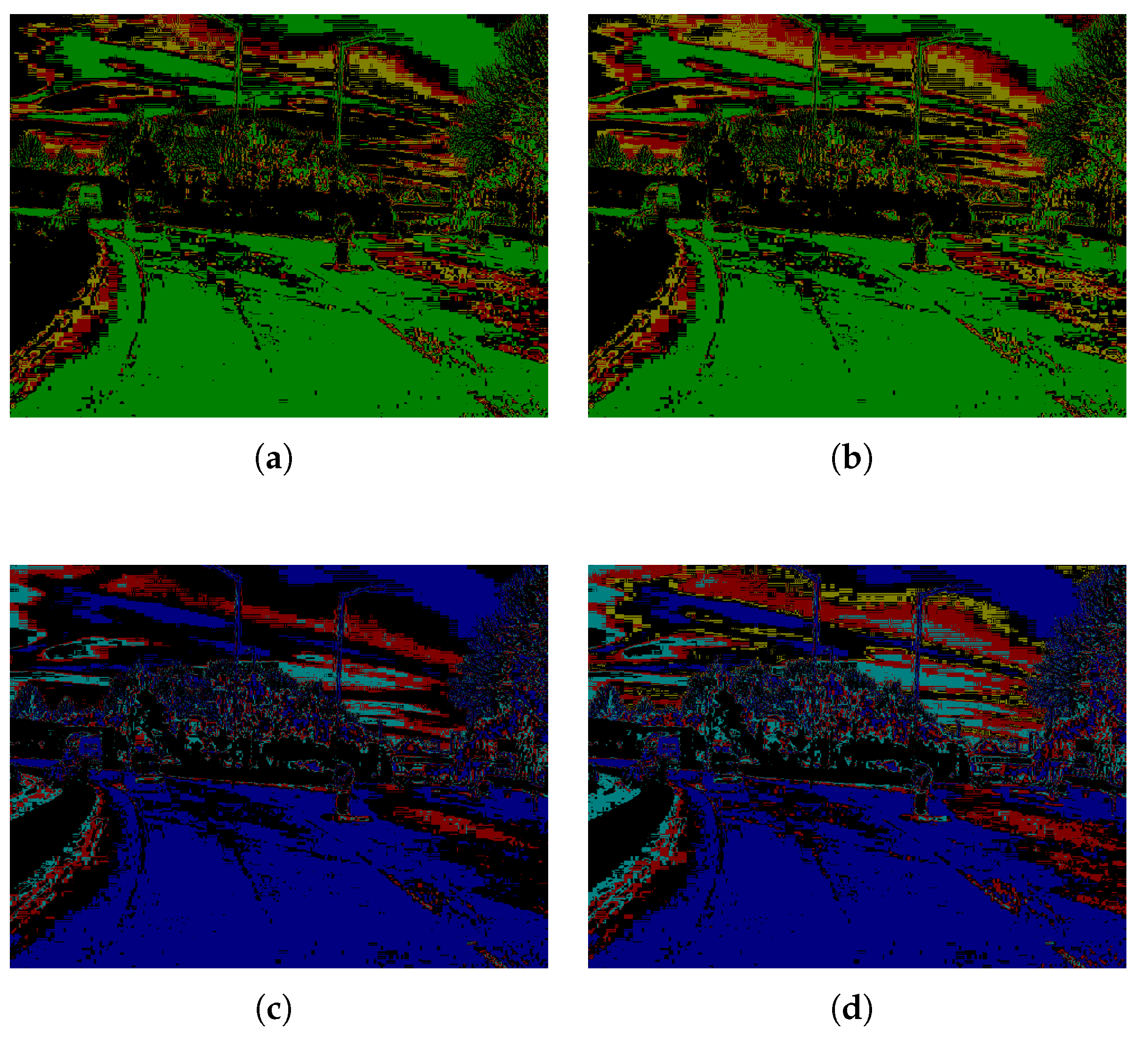
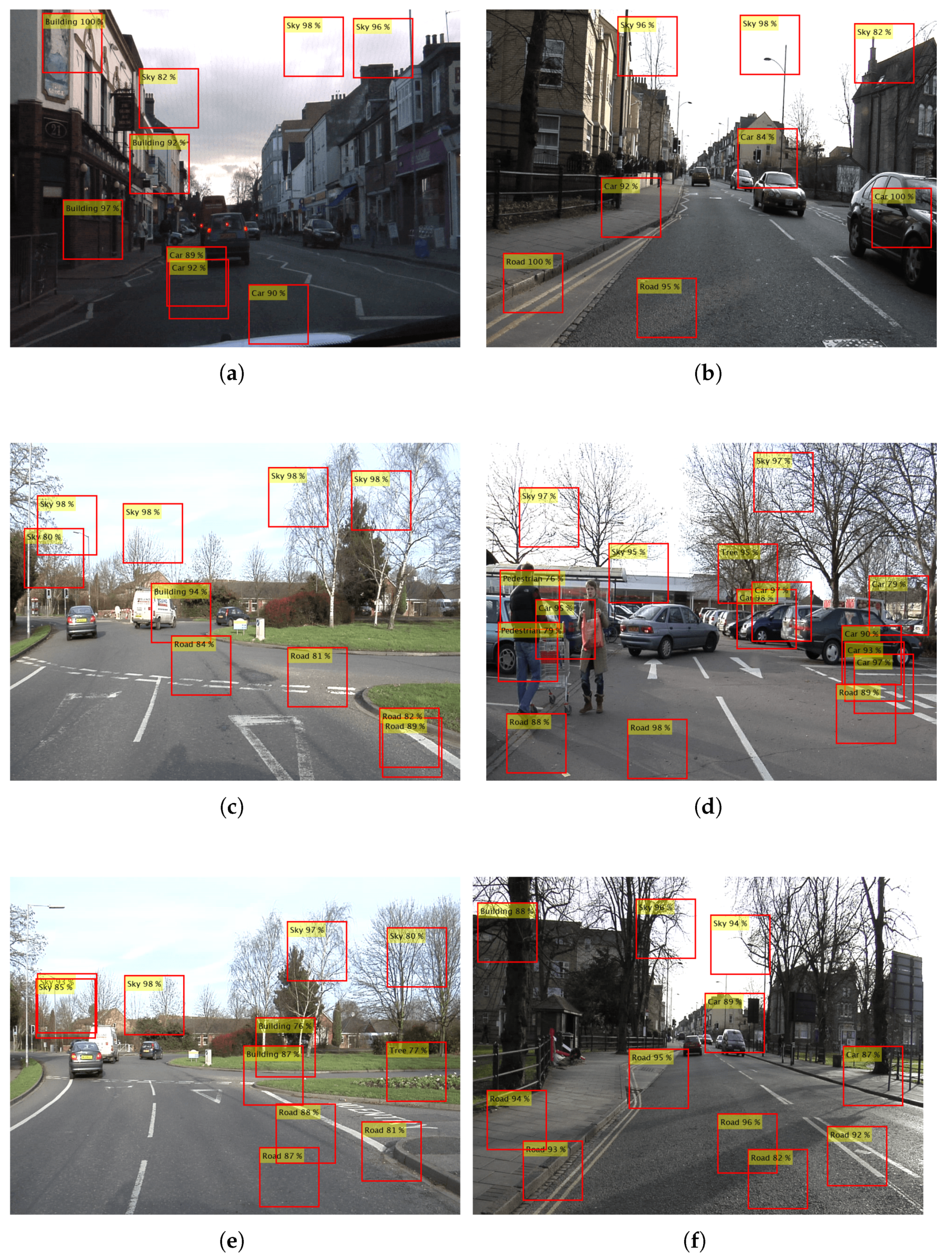
4.1. Experimental Results

Segmentation and classification results are obtained using Cityscape [28] and CamVid [29] datasets. Similar datasets, i.e., Kitti, Waymo [30], and nuScenes [31], are used for 2 D and 3 D object detection for self-driving. The Cityscape dataset is divided into 20 folders obtained from several European cities; in this case, the Munster subfolder with 174 images of 1024 × 2048 pixels was chosen. In contrast, the CamVid dataset has 701 images of 720 × 960 pixels. Both datasets showed urban contexts but under different seasonal and lighting conditions.
The color image and the number of blocks on the chromatic map are the inputs for the segmentation algorithm. Each input image is processed using 16 different blocks, generating 16 segmented images. Each segmented image is colored by area according to the values of a 256−color map. Figure 6 and Figure 7 show the segmentation results for an image taken from the CamVid dataset, using different block sizes on the chromatic map. The validation method used shows that the chromatic map for the CamVid dataset produces better results in a ( 8 × 16 ) combination, unlike the Cityscape database, which produced better results for ( 16 × 8 ) values, as shown in the following subsection.

4.2. Segmentation Performance

The number of representative areas segmented is validated through a quantitative analysis of ground-truth images provided by Cityscape and CamVid datasets. Table 1 shows the number of representative areas n t h found by Algorithm 1 for various block sizes on the chromatic map. Bear in mind that as the number of blocks on the axes increases, the number of representative areas increases too. Segmented images can be empty in both cases, meaning no representative area was found.
A second validation of segmented images consists of selecting the most common categories and their semantics to compare with the segmented areas. The most common categories from the urban context are enough for a general description of the scene. The selected categories are building, car, pedestrian, road, sky, and tree. Each segmented image is analyzed by area. The results for categories building, pedestrian, and road using the CamVid dataset are shown in Table 2, and those using the Cityscape dataset are shown in Table 3. Both tables show the segmented pixel-by-pixel relationship between the results and the ground-truth images, which makes it possible to consider some criteria to establish block sizes ( m , n ):
  • The percentage of pixel relationship by a class must be at least 50 % similar to ground-truth.
  • Reject block sizes on m , n where the number of void images is higher than 10%.
Therefore, m , n block sizes where m n are used to comply with the last criterion, and the number of areas are enough to represent the categories.

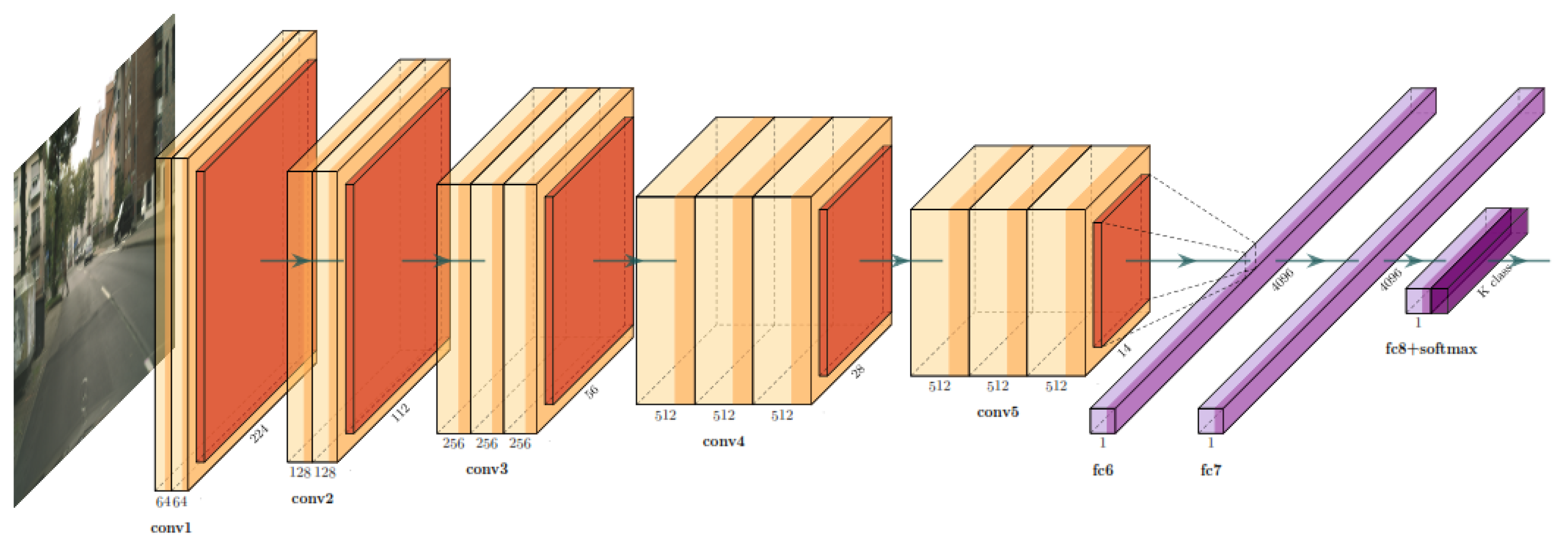
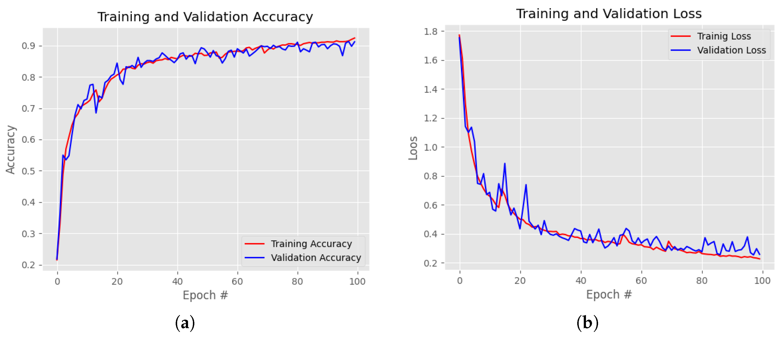
4.3. Cnn Architecture

Figure 8 shows network architecture based on VGG-16 [32] used in this study. This architecture has 16 layers to train about 138 million of parameters. The network consists of five blocks of convolutional layers. Each block consists of two or three convolutional layers followed by a groping layer. The number of filters increases by 2, from 64 to 512. The Dropout layers are added between one block and the next to avoid over-adjustment [33]. Each Dropout layer reduces the connection between one block and the next. The flat layer connects convolutional blocks with the fully connected layer. The fully connected layers have 4096 neurons, including “bias” and the activation function, a ReLU in this case. The last fully connected layer is the output from the network. The number of neurons on this layer is the same as the number of categories. The activation function associated with the last fully connected layer is the Softmax or normalized exponential function for a multi-class problem.
Algorithm 1 calculates the segmentation of input images used to process the training and validation dataset. This process is illustrated in Figure 9. A binary mask per category, known as class mask, is generated for each image on the dataset. The class mask is then used to crop p patches randomly sized [ l u × l v ] = [ 60 × 80 ] for each category. About 30,000 patches were generated for all the classes using the Cityscape database, with approximately 3000 images.
All patches were resized to [ 96 × 96 ] , [ 128 × 128 ] and [ 224 × 224 ] for use on the CNN. Figure 10a,b show the accuracy and loss chart, respectively, for training of 100 epochs using an image size of ( 224 × 224 ) .
The SmallVGG network model was also used to optimize its resources and keep performance results optimal. This network model reduces the original architecture presented in this study [32]. Even though the VGG-16 model for a resized 96 × 96 path shows greater accuracy than the results shown in Table 4, 224 × 224 images have had a more stable performance during the training and validation phase.
Additional experimental tests were performed using the ResNet CNN model, and the results are included in Table 4. In [34], the authors describe the residual blocks used for training deeper layers in the network. Using skip connections, it is possible to activate one layer and relocate its output to feed deeper layers in the network. ResNet CNN architectures are built by grouping a set of residual blocks. It is important to point out that the adder in the residual block can only be performed if both layers have the same dimension. For six categories and three different sizes of patches, we obtained an accuracy of 94 % for 224 × 224 image patches.
The network model is validated using a training dataset from segmented images. Ground-truth information is not used with the validation dataset, and therefore, patches generated depend only on the areas obtained from the segmented image and the equivalent input color image. Unlike the training dataset, these patches are chosen randomly by area and do not have a predetermined category. This is represented visually in Figure 11. The patches are cropped from the color image using a fixed size [ l u × l v ] = [ 224 × 224 ] , which is the classifier input size. A different number of patches is cropped for each segmented area depending on the size and the number of regions obtained. The fixed size of bounding boxes allows the classification of undefined categories, such as sky and road, which most object-detect methodologies cannot detect and classify. This is one of our contributions to classifiers in urban environments.
Experimental tests to validate this approach use patches generated using the CamVid dataset. The classifier assigns a label and a reliability label to each patch. The output image shows different boundary frames with the brand and the reliability value corresponding to each image patch. Some results are shown in Figure 12. The CNN architecture was trained using the CityScape dataset, which has bigger images, and therefore, the process of generating patches was more straightforward.
Experimental tests were conducted using a PC with Intel Core i5 9th generation, 32 GB of RAM, and an NVIDIA GeForce GTX 1650 graphics card. Table 5 shows the time for the segmentation algorithm.
Bear in mind that the time presented in Table 5 depends on the number of areas on the segmented image and their sizes. When a patch for an area cannot be obtained, this increases processing time significantly. To limit the execution time, a maximal number of tries to generate the patches has been established. In addition, the number of patches per image depends on the number of representative areas obtained by the segmentation algorithm for each image divided into four partitions (see Figure 11). Thus, the number of patches changes from image to image, and so does the total processing time. Processing times were analyzed, including those recorded in the classification phase. Table 6 shows the number of patches generated and the time. A general processing time per image can be produced by adding the segmentation and classification times. For instance, the time for the CamVid dataset is 4 seconds; for the CityScape image, it is twice as long.

5. Discussion

Table 7 shows a comparison between our proposal and other methodologies in the literature. Using ResNet, we achieve 94 % accuracy, whereas YOLOv3 [35] and YOLOv4 [36] architecture achieve over 95 % accuracy for the ImageNet dataset. Different approaches compared were VOLO [25] and SPPNet [37], which also achieved good accuracy in the top rate. Even if our classification accuracy is lower, in this work, we provide an alternative method to classify image content without performing a whole refined segmentation of the image and without using semantic image information. Therefore, sky and road classes have been included as categories. In contrast, YOLO or other object classification architectures do not consider it because a bounding box cannot be defined for both categories.
Our accuracy results also depend on the bounding-boxes size extracted from the image; note in Table 4 that our accuracy increases as this selected size does. Our methodology is an alternative region-based approach that has been trained with one dataset and validated with another. Both datasets only have the urban context in common, but resolution and illumination are different, becoming more difficult for the validation task.
A final experimental test was performed by training boosted trees and several machine learning classifiers using the patches extracted from our method; the obtained results are illustrated in Table 8. For six categories and three different sizes, the highest accuracy was 79.80 % , achieved by the Bagged Trees classifier. Considering that CNN architectures extract the main and representative features through the layers, machine learning-based classifiers require a more careful feature extractor strategy to improve their classification accuracy.

6. Conclusions

This study shows a new approach to image segmentation to identify objects in structured outdoor spaces. The approach extracts representative features based on combining algebra for complex numbers on planes a and b on the CIELab color space. The complex image makes it possible to develop and implement a multi-threshold segmentation algorithm. The methodology follows a typical automatic learning technique. The required features to input the classifier are chosen from specific areas on the segmented image. Despite light and overcrowding issues in outdoor environments, the number of classes and images used in the training and validation phases of the model are enough to execute the identification of objects.
The multi-threshold segmentation algorithm produces different execution time lapses depending on the image features to be processed. This is also dependent on the computing power available. In addition, the different sets of images used for CNN training and validation are created using random conditions. The execution time results for the multi-threshold segmentation algorithm depend on the size and features of the image. Thus far, this approach cannot be used in real-time conditions that require execution speeds of milliseconds. However, a dispersal strategy to select different areas on the scene could provide lighter techniques for classification purposes. Given the modular nature of the methodology, modifications to increase hardware performance are possible.
The VGG-16 network responds well to conditions such as those in this study, showing a uniform and flexible architecture; however, better accuracy results were achieved using the ResNet-150 network. Execution times for classification purposes are affected by the various phases in the methodology and the different features of the images from the databases. Hence, the decision to train the CNN architecture using the Cityscape dataset and validate it using the CamVid dataset shows similar outdoor and urban environments.
Finally, this study has focused on a less computationally intensive alternative to conducting color segmentation and object detection tasks, with the flexibility of adapting to different hardware architectures and scenarios.

Author Contributions

Conceptualization, D.-L.A.-O. and M.-A.I.-M.; methodology, D.-A.R.-M. and D.-L.A.-O.; software, J.-J.C.-C. and M.-A.I.-M.; validation, J.-J.C.-C. and D.-A.R.-M.; formal analysis, J.-J.C.-C., D.-L.A.-O. and M.-A.I.-M.; investigation, J.-J.C.-C. and D.-A.R.-M.; data curation, J.-J.C.-C. and D.-L.A.-O.; writing—original draft preparation, J.-J.C.-C.; writing—review and editing, D.-L.A.-O. and M.-A.I.-M.; visualization, D.-L.A.-O., D.-A.R.-M. and M.-A.I.-M.; project administration, D.-L.A.-O. All authors have read and agreed to the published version of the manuscript.

Funding

This study was conducted as part of the doctoral studies of Juan-Jose Cardenas-Cornejo, funded through scholarship number 2021-000018-02NACF-07210, awarded by CONACYT.

Data Availability Statement

Not applicable.

Acknowledgments

The authors are grateful to the University of Guanajuato. The authors would like special thanks to Carlos Montoro for his technical support in the English revision of the manuscript.

Conflicts of Interest

The authors declare no conflict of interest.

References

  1. Yurtsever, E.; Lambert, J.; Carballo, A.; Takeda, K. A Survey of Autonomous Driving: Common Practices and Emerging Technologies. IEEE Access 2020, 8, 58443–58469. [Google Scholar] [CrossRef]
  2. Narkhede, P.R.; Gokhale, A.V. Color image segmentation using edge detection and seeded region growing approach for CIELab and HSV color spaces. In Proceedings of the 2015 International Conference on Industrial Instrumentation and Control (ICIC), Pune, India, 28–30 May 2015. [Google Scholar] [CrossRef]
  3. Xu, Y.; Shen, B.; Zhao, M.; Luo, S. An Adaptive Robot Soccer Image Segmentation Based on HSI Color Space and Histogram Analysis. J. Comput. 2019, 30, 290–303. [Google Scholar]
  4. Smith, A.R. Color gamut transform pairs. In Proceedings of the SIGGRAPH ’78, Atlanta, GA, USA, 23–25 August 1978. [Google Scholar]
  5. Cheng, H.D.; Jiang, X.H.; Sun, Y.; Wang, J. Color Image Segmentation: Advances and Prospects. Pattern Recognit. 2001, 34, 2259–2281. [Google Scholar] [CrossRef]
  6. Bansal, S.; Aggarwal, D. Color image segmentation using CIELab color space using ant colony optimization. Int. J. Comput. Appl. Citeseer 2011, 29, 28–34. [Google Scholar] [CrossRef]
  7. Spiegel, M.R.; Seymour Lipschutz, J.J.S.; Spellman, D. Complex Variables: With an Introduction to Conformal Mapping and Its Applications, 2nd ed.; Schaum’s Outlines Series; McGraw-Hill: New York, NY, USA, 2009. [Google Scholar]
  8. Fujiyoshi, H.; Hirakawa, T.; Yamashita, T. Deep learning-based image recognition for autonomous driving. IATSS Res. 2019, 43, 244–252. [Google Scholar] [CrossRef]
  9. Xu, H.; Gao, Y.; Yu, F.; Darrell, T. End-To-End Learning of Driving Models From Large-Scale Video Datasets. In Proceedings of the IEEE Conference on Computer Vision and Pattern Recognition (CVPR), Honolulu, HI, USA, 21–26 July 2017. [Google Scholar]
  10. Dal Mutto, C.; Zanuttigh, P.; Cortelazzo, G.M. Fusion of geometry and color information for scene segmentation. IEEE J. Sel. Top. Signal Process. 2012, 6, 505–521. [Google Scholar] [CrossRef]
  11. Pagnutti, G.; Zanuttigh, P. Joint segmentation of color and depth data based on splitting and merging driven by surface fitting. Image Vis. Comput. 2018, 70, 21–31. [Google Scholar] [CrossRef] [Green Version]
  12. Karimpouli, S.; Tahmasebi, P. Segmentation of digital rock images using deep convolutional autoencoder networks. Comput. Geosci. 2019, 126, 142–150. [Google Scholar] [CrossRef]
  13. Rochan, M.; Rahman, S.; Bruce, N.D.; Wang, Y. Weakly supervised object localization and segmentation in videos. Image Vis. Comput. 2016, 56, 1–12. [Google Scholar] [CrossRef]
  14. Zhou, D.; Frémont, V.; Quost, B.; Dai, Y.; Li, H. Moving object detection and segmentation in urban environments from a moving platform. Image Vis. Comput. 2017, 68, 76–87. [Google Scholar] [CrossRef]
  15. Xie, J.; Kiefel, M.; Sun, M.T.; Geiger, A. Semantic Instance Annotation of Street Scenes by 3D to 2D Label Transfer. In Proceedings of the Conference on Computer Vision and Pattern Recognition (CVPR), Las Vegas, NV, USA, 27–30 June 2016. [Google Scholar]
  16. Kaushik, R.; Kumar, S. Image Segmentation Using Convolutional Neural Network. Int. J. Sci. Technol. Res. 2019, 8, 667–675. [Google Scholar]
  17. Ye, X.Y.; Hong, D.S.; Chen, H.H.; Hsiao, P.Y.; Fu, L.C. A two-stage real-time YOLOv2-based road marking detector with lightweight spatial transformation-invariant classification. Image Vis. Comput. 2020, 102, 103978. [Google Scholar] [CrossRef]
  18. Long, J.; Shelhamer, E.; Darrell, T. Fully convolutional networks for semantic segmentation. In Proceedings of the IEEE Conference on Computer Vision and Pattern Recognition, Boston, MA, USA, 7–12 June 2015; pp. 3431–3440. [Google Scholar]
  19. Noh, H.; Hong, S.; Han, B. Learning Deconvolution Network for Semantic Segmentation. In Proceedings of the IEEE International Conference on Computer Vision (ICCV), Santiago, Chile, 7–13 December 2015. [Google Scholar]
  20. Chen, L.C.; Papandreou, G.; Kokkinos, I.; Murphy, K.; Yuille, A.L. Deeplab: Semantic image segmentation with deep convolutional nets, atrous convolution, and fully connected crfs. IEEE Trans. Pattern Anal. Mach. Intell. 2017, 40, 834–848. [Google Scholar] [CrossRef] [Green Version]
  21. He, K.; Gkioxari, G.; Dollár, P.; Girshick, R. Mask r-cnn. In Proceedings of the IEEE International Conference on Computer Vision, Venice, Italy, 22–29 October 2017; pp. 2961–2969. [Google Scholar]
  22. Ren, S.; He, K.; Girshick, R.; Sun, J. Faster R-CNN: Towards Real-Time Object Detection with Region Proposal Networks. IEEE Trans. Pattern Anal. Mach. Intell. 2017, 39, 1137–1149. [Google Scholar] [CrossRef] [PubMed] [Green Version]
  23. Rehman, S.; Ajmal, H.; Farooq, U.; Ain, Q.U.; Riaz, F.; Hassan, A. Convolutional neural network based image segmentation: A review. In Proceedings of the Pattern Recognition and Tracking XXIX, Orlando, FL, USA, 15–19 April 2018. [Google Scholar] [CrossRef]
  24. Li, Q.; Shen, L.; Guo, S.; Lai, Z. Wavelet integrated CNNs for noise-robust image classification. In Proceedings of the IEEE/CVF Conference on Computer Vision and Pattern Recognition, Seattle, WA, USA, 13–19 June 2020; pp. 7245–7254. [Google Scholar]
  25. Yuan, L.; Hou, Q.; Jiang, Z.; Feng, J.; Yan, S. Volo: Vision outlooker for visual recognition. IEEE Trans. Pattern Anal. Mach. Intell. 2022, 1–13. [Google Scholar] [CrossRef] [PubMed]
  26. Wu, Y.H.; Liu, Y.; Zhan, X.; Cheng, M.M. P2T: Pyramid pooling transformer for scene understanding. IEEE Trans. Pattern Anal. Mach. Intell. 2022, 1–12. [Google Scholar] [CrossRef] [PubMed]
  27. Churchill, R.V.; Brown, J.W. Variable Compleja y Aplicaciones, 5th ed.; McGraw-Hill-Interamericana: Madrid, Spain, 1996. [Google Scholar]
  28. Cordts, M.; Omran, M.; Ramos, S.; Rehfeld, T.; Enzweiler, M.; Benenson, R.; Franke, U.; Roth, S.; Schiele, B. The Cityscapes Dataset for Semantic Urban Scene Understanding. In Proceedings of the IEEE Conference on Computer Vision and Pattern Recognition (CVPR), Las Vegas, NV, USA, 27–30 June 2016; pp. 3213–3223. [Google Scholar]
  29. Brostow, G.J.; Fauqueur, J.; Cipolla, R. Semantic object classes in video: A high-definition ground truth database. Pattern Recognit. Lett. 2009, 30, 88–97. [Google Scholar] [CrossRef]
  30. Sun, P.; Kretzschmar, H.; Dotiwalla, X.; Chouard, A.; Patnaik, V.; Tsui, P.; Guo, J.; Zhou, Y.; Chai, Y.; Caine, B.; et al. Scalability in Perception for Autonomous Driving: Waymo Open Dataset. In Proceedings of the IEEE/CVF Conference on Computer Vision and Pattern Recognition (CVPR), Seattle, WA, USA, 13–19 June 2020; pp. 2446–2454. [Google Scholar]
  31. Caesar, H.; Bankiti, V.; Lang, A.H.; Vora, S.; Liong, V.E.; Xu, Q.; Krishnan, A.; Pan, Y.; Baldan, G.; Beijbom, O. nuScenes: A multimodal dataset for autonomous driving. In Proceedings of the CVPR, Seattle, WA, USA, 13–19 June 2020; pp. 11621–11631. [Google Scholar]
  32. Simonyan, K.; Zisserman, A. Very deep convolutional networks for large-scale image recognition. In Proceedings of the 3rd International Conference on Learning Representations, ICLR 2015—Conference Track Proceedings, San Diego, CA, USA, 7–9 May 2015; pp. 1–14. [Google Scholar]
  33. Srivastava, N.; Hinton, G.; Krizhevsky, A.; Sutskever, I.; Salakhutdinov, R. Dropout: A simple way to prevent neural networks from overfitting. J. Mach. Learn. Res. JMLR. Org 2014, 15, 1929–1958. [Google Scholar]
  34. He, K.; Zhang, X.; Ren, S.; Sun, J. Deep residual learning for image recognition. In Proceedings of the IEEE Conference on Computer Vision and Pattern Recognition, Las Vegas, NV, USA, 27–30 June 2016; pp. 770–778. [Google Scholar]
  35. Redmon, J.; Farhadi, A. Yolov3: An incremental improvement. arXiv 2018, arXiv:1804.02767. [Google Scholar]
  36. Bochkovskiy, A.; Wang, C.Y.; Liao, H.Y.M. Yolov4: Optimal speed and accuracy of object detection. arXiv 2020, arXiv:2004.10934. [Google Scholar]
  37. He, K.; Zhang, X.; Ren, S.; Sun, J. Spatial pyramid pooling in deep convolutional networks for visual recognition. IEEE Trans. Pattern Anal. Mach. Intell. 2015, 37, 1904–1916. [Google Scholar] [CrossRef]
Figure 1. Proposed segmentation method to identify objects.
Mathematics 10 03752 g001
Figure 2. Generating complex image I using the chromatic images i m A and i m B .
Mathematics 10 03752 g002
Figure 3. Complex division using a representative chromatic point.
Mathematics 10 03752 g003
Figure 4. Chromatic map AB for two color images. (a) Color image 1. (b) Chromatic map AB of image 1. (c) Color image 2. (d) Chromatic map AB of image 2.
Mathematics 10 03752 g004
Figure 5. Chromatic map AB divided into m × n blocks on the chromatic range given by Δ a and Δ b .
Mathematics 10 03752 g005
Figure 6. CamVid segmented images for different block sizes. (a) Block size 4 × 8 . (b) Block size 4 × 16 . (c) Block size 8 × 8 . (d) Block size 8 × 16 .
Mathematics 10 03752 g006
Figure 7. CamVid segmented images for different block sizes. (a) Block size 16 × 8 . (b) Block size 16 × 16 . (c) Block size 32 × 8 . (d) Block size 32 × 16 .
Mathematics 10 03752 g007
Figure 8. Modified convolutional neural network VGG-16.
Mathematics 10 03752 g008
Figure 9. Class mask obtained from a segmented image to generate patches for the category building. A similar process is followed for all the categories to process the training dataset.
Mathematics 10 03752 g009
Figure 10. Results from training the CNN using 224 × 224 images. (a) Accuracy graph. (b) Loss graph.
Mathematics 10 03752 g010
Figure 11. Image patches generated to validate the classifier.
Mathematics 10 03752 g011
Figure 12. Classification of objects using CamVid. (a) Test image #1. (b) Test image #2. (c) Test image #3. (d) Test image #4. (e) Test image #5. (f) Test image #6.
Mathematics 10 03752 g012
Table 1. Number of representative areas generated by each dataset.
Y b -Axis BlocksCityscape ImageCamVid Image
X a -Axis Blocks X a -Axis Blocks
481632481632
4347112469
8447114459
166671366610
321211121211111013
Table 2. Analysis of segmented image categories for CamVid.
Class Y b -Axis Blocks X a -Axis Blocks
4 8 16 32
Pixel RatioVoid ImagesPixel RatioVoid ImagesPixel RatioVoid ImagesPixel RatioVoid Images
Building4 0.2049 464 0.4277 227 0.622 28 0.6215 14
8 0.4415 212 0.4982 162 0.6190 20 0.6050 14
16 0.5459 15 0.5488 16 0.5397 14 0.5369 14
32 0.5337 14 0.5358 14 0.5149 14 0.4843 14
Pedestrian4 0.1984 486 0.3865 267 0.5604 75 0.5437 61
8 0.4253 249 0.4705 202 0.5572 68 0.5377 61
16 0.5714 62 0.5736 63 0.5497 61 0.5321 61
32 0.5551 62 0.5482 61 0.5167 61 0.4812 61
Road4 0.3461 457 0.6155 214 0.7846 14 0.7546 0
8 0.6260 202 0.6697 150 0.7521 7 0.7155 0
16 0.7147 1 0.6807 2 0.6488 0 0.6048 0
32 0.6058 0 0.6056 0 0.5788 0 0.5591 0
Table 3. Analysis of segmented image categories for CityScape.
Class Y b -Axis Blocks X a -Axis Blocks
4 8 16 32
Pixel RatioVoid ImagesPixel RatioVoid ImagesPixel RatioVoid ImagesPixel RatioVoid Images
Building4 0.1427 130 0.3275 73 0.4355 4 0.4390 4
8 0.5105 45 0.4697 47 0.4903 4 0.4620 4
16 0.6817 4 0.6406 4 0.5418 4 0.4652 4
32 0.7239 4 0.6817 4 0.5853 4 0.4850 4
Pedestrian4 0.0885 139 0.2179 94 0.2982 38 0.3068 38
8 0.4251 71 0.3635 73 0.3843 38 0.4253 38
16 0.5761 38 0.5494 38 0.4741 38 0.4704 38
32 0.6114 38 0.5885 38 0.5278 38 0.4439 38
Road4 0.2277 128 0.4983 71 0.7376 2 0.6822 2
8 0.6493 43 0.6222 45 0.7327 2 0.6284 2
16 0.8533 2 0.8310 2 0.7321 2 0.5709 2
32 0.8346 2 0.8063 2 0.7089 2 0.6295 2
Table 4. CNN accuracy results for different image sizes.
ArchitectureImage Size (in Pixels)
96 × 96 128 × 128 224 × 224
SmallVGG 0.73 0.82 0.87
VGG16-Modified 0.92 0.90 0.91
ResNet150 0.26 0.81 0.94
Table 5. Execution time for the segmentation algorithm.
DatasetExecution Time (in Seconds)
Per ImageTotal No. of Images Per Dataset
CamVid 0.83187 394.0215
Cityscape 3.07230 4662.554
Table 6. Classification execution time.
DatasetNumber of Patches GeneratedExecution Time (in Seconds)
Per ImageTotal No. of Images on Dataset
CamVid11,660 2.9092 889.5841
Cityscape2883 5.2499 245.0659
Table 7. Comparison with related works.
WorkMethodologyDatasetAccuracy
YOLOv3 [35]
YOLOv4 [36]
An integrated CNN’s used for feature extraction and object classification in real-time.ImageNet93.8%
94.8%
Top-5
accuracy rate
VOLO [25]A new architecture that implements a novel outlook attention operation that dynamically conducts the local feature aggregation mechanism in a sliding window manner across the input image.ImageNet87.1%
Top-1
accuracy rate
SPPNet [37]Strategy of spatial pyramid pooling to construct a network structure called SPP-net for image classification.Caltech10193.42%
Our
approach
Selection of region chromatic based on complex numbers with CNN to object detection.Cityscapes
and
Camvid
94%
for
6 classes
Table 8. Classification result using machine learning approaches.
Classification LearnerPatches Sizes (in Pixels)
96 × 96 128 × 128 224 × 224
Quadratic SVM78.10%78.30%78.90%
Cubic SVM78.50%79.10%80.10%
Fine Gaussian SVM67.30%70.20%74.10%
Medium Gaussian SVM77.80%77.80%77.40%
Bagged Trees79.20%79.40%79.80%
Narrow Neural Network72.90%74.20%76.20%
Medium Neural Network74.60%76.60%78.70%
Bilayered Neural Network72.90%74.20%77.00%
Trilayered Neural Network73.70%74.60%76.10%
Publisher’s Note: MDPI stays neutral with regard to jurisdictional claims in published maps and institutional affiliations.

